A Three-Dimensional Model of the Marine Nitrogen Cycle during the Last Glacial Maximum Constrained by Sedimentary Isotopes

Introduction

The global nitrate (${\text{NO}}_3^{-}$) inventory regulates marine productivity and sequestration of carbon in the deep ocean via sinking organic matter (i.e., the biological pump). In the modern ocean, ${\text{NO}}_3^{-}$ is the main limiting nutrient throughout the tropical and subtropical oceans (Moore et al., 2013) because N-loss processes cause its depletion relative to other macronutrients such as phosphate (${\text{PO}}_4^{3-}$). Therefore, significant changes to the global ${\text{NO}}_3^{-}$ inventory, which is known to be sensitive to climate (Gruber and Galloway, 2008), may feedback on climate via the biological pump.

The predominant source of bioavailable fixed nitrogen (N) to the ocean is N₂ fixation by specialized cyanobacteria (diazotrophs) capable of converting dinitrogen gas to ammonium to meet their nitrogen requirements for growth. N₂ fixation has extra energy requirements relative to assimilating forms of fixed nitrogen associated with breaking down the triple N bond in dinitrogen, extra respiration requirements to keep the N₂-fixing cellular compartment anoxic, as well as additional structural iron requirements of the N₂-fxing nitrogenase enzyme (e.g., see Karl et al., 2002; Grosskopf and Laroche, 2012).

Nitrogen loss (N-loss) processes occur in oxygen deficient zones (ODZs, O₂ <~10 mmol m⁻³) where ${\text{NO}}_3^{-}$ replaces O₂ as the electron acceptor during organic matter respiration. Under these suboxic conditions, forms of fixed nitrogen (NH₄, NO₂, ${\text{NO}}_3^{-}$) are converted to N₂O and N₂ gas primarily by heterotrophic denitrification and autotrophic anammox. These N-loss processes occur both in the pore-water sediments and marine water column. Previous estimates suggest that the global ratio of sedimentary to water column N-loss is between 1 and 4 (Brandes and Devol, 2002; Altabet, 2007; Codispoti, 2007), with more recent modeling efforts suggesting a narrower range of 1.3–2.3 (Eugster and Gruber, 2012; Devries et al., 2013; Somes et al., 2013).

The balance between N₂ fixation and N-loss mainly determines the preindustrial global ${\text{NO}}_3^{-}$ inventory. In the preindustrial Late Holocene (0–5,000 years ago), these processes were likely close to balanced (Gruber, 2008), which has also been interpreted from the stability of sedimentary nitrogen isotope records during this period (Altabet, 2007). Some estimates have suggested that present-day N-loss processes may be much larger than N₂ fixation, leading to an anthropogenic ocean that could be rapidly losing N (Codispoti, 2007). However, methodological issues with historical N₂ fixation measurements suggest a significant underestimation of N₂ fixation by at least a factor of 2 (Mohr et al., 2010; Großkopf et al., 2012), which could explain much of the large imbalance in some previous budgets. Recent modeling efforts (Eugster and Gruber, 2012; Devries et al., 2013) have estimated global N-loss rates (120–240 Tg N yr⁻¹) that are on the low-end of previous studies that suggest as high as 400 Tg N yr⁻¹ (Codispoti, 2007), again suggesting previous budgets should be closer to balanced.

Isotope ratios of nitrogen (¹⁵R_N =¹⁵N/¹⁴N), typically reported as delta values (δ¹⁵N = ¹⁵R_N/¹⁵R_{N, std}−1), can be used to infer changes in physical and biogeochemical processes related to nitrogen cycling (Wada, 1980). δ¹⁵${\text{NO}}_3^{-}$ is strongly fractionated by water column N-loss, preferentially removing ¹⁴N thus increasing δ¹⁵${\text{NO}}_3^{-}$ of the remaining nitrate (ε_WCNl = 15–30‰; Cline and Kaplan, 1975). Sedimentary N-loss has a lower isotope effect (ε_SedNl = 1.5–13‰; Brandes and Devol, 1997; Lehmann et al., 2007; Granger et al., 2011; Dale et al., 2014) due to more complete ${\text{NO}}_3^{-}$ utilization in pore-water sediments compared to typical water column conditions. N₂ fixation introduces ¹⁵N-depleted nitrogen (δ¹⁵N_Nfix = −1‰; Minagawa and Wada, 1986), thereby decreasing δ¹⁵${\text{NO}}_3^{-}$, which is ~5‰ on average globally (Sigman et al., 2000; Somes et al., 2010). Phytoplankton assimilate ¹⁴N more efficiently than ¹⁵N (${\epsilon }_{{\text{NO}}_3^{-}\text{upt}}$ = 5–10‰; Wada and Hattori, 1978), which increases δ¹⁵${\text{NO}}_3^{-}$ of the residual ${\text{NO}}_3^{-}$ and has a large effect in N-depleted surface waters in the absence of N₂ fixation. Zooplankton excrete ¹⁵N-depleted nitrogen causing their biomass to be enriched by 3–4‰ relative to their prey (Minagawa and Wada, 1984), causing the step-wise enrichment of δ¹⁵N through higher tropic levels.

δ¹⁵N measured in the water column and on sedimentary organic matter has been used to reconstruct changes in nitrogen cycling from previous climate periods (Robinson et al., 2012). δ¹⁵N records are typically interpreted qualitatively as changes to nutrient utilization in modern High Nitrate Low Chlorophyll (HNLC) regions, water column N-loss, or N₂ fixation (e.g., Altabet and Francois, 1994; Altabet et al., 1995; Ren et al., 2009). However, nitrogen isotope ratios are influenced by a variety of biogeochemical processes, sometimes at the same location, including transport by the circulation and mixing (Schmittner and Somes, 2016), which complicates their ability to quantitatively constrain nitrogen cycling processes based on individual sediment cores alone.

During the Last Glacial Maximum (LGM) ~21,000 years before present, lower temperatures have presumably increased solubility of oxygen and improved oxygen supply to the upper ocean ODZs (Jaccard and Galbraith, 2012), thereby reducing water column N-loss. Sedimentary N-loss was also likely reduced during the LGM due to exposed continental shelves from lower sea level (McElroy, 1983; Christensen et al., 1987). In the modern ocean approximately half of total sedimentary N-loss is estimated to occur on these shallow continental shelves (Bohlen et al., 2012). Previous box modeling studies using sedimentary δ¹⁵N as a constraint to estimate that total N-loss increased by ~30–120% across the last deglaciation (Deutsch et al., 2001; Eugster et al., 2013; Galbraith et al., 2013). However, more realistic, three-dimensional models have not been used so far to quantify these effects and their impacts on the global nitrogen inventory.

Effects of glacial conditions on N₂ fixation are more uncertain. Falkowski (1997) suggests that increased atmospheric Fe deposition to the glacial ocean stimulated additional N₂ fixation that could have increased the global ${\text{NO}}_3^{-}$ inventory. Broecker (1982), and more recently (Wallmann et al., 2016) propose that a higher ${\text{PO}}_4^{3-}$ inventory, due to reduced loss on continental shelves, could have enhanced N₂ fixation during the LGM since ${\text{PO}}_4^{3-}$ is diazotrophs' other main limiting nutrient. On the other hand, Ren et al. (2009, 2012) interpret δ¹⁵N records from the western tropical North Atlantic and Pacific as reduced N₂ fixation, in response to lower N-loss in the glacial ocean. Some specific N₂-fixing Trichodesmium species may also be limited by CO₂ concentrations of surface waters (Barcelos e Ramos et al., 2007; Hutchins et al., 2007), which could have reduced N₂ fixation during the LGM, although other studies investigating Trichodesmium community assemblages (Gradoville et al., 2014) and unicellular diazotrophs (Law et al., 2012) found no consistent effect of CO₂ on N₂ fixation.

Previous box modeling studies have produced large differences in their estimates of the global ${\text{NO}}_3^{-}$ inventory during the LGM, ranging from < +10% (Deutsch et al., 2004) up to +100% (Eugster et al., 2013). The lower estimates would imply negligible impacts on the carbon cycle and atmospheric CO₂, whereas the higher estimates could lead to enhanced atmospheric CO₂ sequestration in the ocean. However, more realistic estimates with three-dimensional models remain lacking. While changes in the oceanic nutrient inventory have been featured in hypotheses put forward to explain the glacial drawdown of atmospheric CO₂ (McElroy, 1983; Christensen et al., 1987; Falkowski, 1997; Broecker and Henderson, 1998), possible effects of changes in the nitrogen inventory on glacial-interglacial CO₂ cycles are sometimes ignored in recent reviews (e.g., Hain et al., 2014) and model simulations (e.g., Brovkin et al., 2007).

Here we present the first three-dimensional model with realistic LGM boundary conditions to estimate changes in N-loss and N₂ fixation and their effects on the nitrogen inventory. We build upon the isotope modeling work of Schmittner and Somes (2016), herein denoted as SS16, which used a global database of sedimentary nitrogen isotopes from the LGM (Tesdal et al., 2012) to constrain idealized 3D LGM simulations. In our global 3D model-data analysis, observations are directly compared to model results at the same locations they represent, rather than defining large, basin-scale averages that previous box modeling studies had to impose. Here we produce more realistic LGM simulations by considering spatially varying atmospheric Fe deposition and sea level effects on sedimentary N-loss, which were not accounted for in SS16. We also provide the first 3D quantitative estimates of effects of hypothesized increases in the ocean's ${\text{PO}}_4^{3-}$ inventory on the nitrogen cycle (Wallmann et al., 2016).

Model Description and Preindustrial Results

We use a slightly modified (see Appendix) model version of SS16, which is based on the UVic Earth System Climate Model (Weaver et al., 2001) with a version of Kiel biogeochemistry (Somes and Oschlies, 2015). In the following we provide a general overview of the model components and their preindustrial results.

Physical Model

The physical ocean-atmosphere-sea ice model includes a three-dimensional (1.8 × 3.6°, 19 vertical levels) general circulation model of the ocean (Modular Ocean Model 2) with parameterizations such as diffusive mixing along and across isopycnals, eddy-induced tracer advection (Gent and McWilliams, 1990), computation of tidally-induced diapycnal mixing over rough topography including sub-grid scale (Schmittner and Egbert, 2014), as well as anisotropic viscosity (Large et al., 2001) and enhanced zonal isopycnal mixing schemes in the tropics to mimic the effect of zonal equatorial undercurrents (Getzlaff and Dietze, 2013). Background vertical mixing is reduced in the tropical subsurface (20°S–20°N, 185–565 m), consistent with microstructure observations and tracer release experiments from the tropical Atlantic (Fischer et al., 2013). A two-dimensional, single level energy-moisture balance atmosphere and a dynamic-thermodynamic sea ice model are used, forced with prescribed monthly climatological winds (Kalnay et al., 1996) and ice sheets (Peltier, 2004). The maximum value of the Atlantic Meridional Overturning Circulation (AMOC) is 17.1 Sv (Figure 1).

FIGURE 1

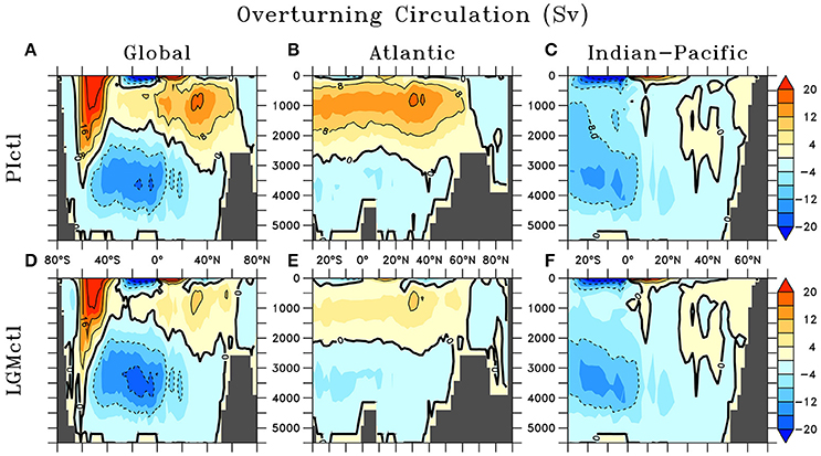
Figure 1. Meridional streamfunction in preindustrial control (PIctl; A–C) and Last Glacial Maximum control (LGMctl; D–F) in the Global, Atlantic, and Indian-Pacific Oceans, respectively.

Marine Biogeochemical Model

The marine ecosystem-biogeochemical model coupled within the ocean circulation includes 2 nutrients in the inorganic (${\text{NO}}_3^{-}$ and ${\text{PO}}_4^{3-}$) and organic (DON and DOP) phases, 2 phytoplankton (ordinary and N₂-fixing diazotrophs), zooplankton, sinking detritus, as well as dissolved O₂, dissolved inorganic carbon, alkalinity, and Δ¹⁴C (Somes and Oschlies, 2015). Iron limitation is calculated using monthly surface dissolved iron fields prescribed from the BLING model (Galbraith et al., 2010). Our model was initialized with World Ocean Atlas (WOA) (Garcia et al., 2010a,b) and the Global Ocean Data Analysis Project (GLODAP; Key et al., 2004) observations and was simulated to quasi steady-state for over 8,000 years under preindustrial boundary conditions. The basin scale patterns of Δ¹⁴C, O₂, and ${\text{NO}}_3^{-}$ are reproduced (Figure S2).

N₂ Fixation

Diazotrophs grow slower than ordinary phytoplankton due to extra energetic demands of N₂-fixation (e.g., Karl et al., 2002; Grosskopf and Laroche, 2012). However, since they have no N-limitation, they can out-compete ordinary phytoplankton in surface waters that are depleted in ${\text{NO}}_3^{-}$, but still contain sufficient P and Fe (e.g., water with low ${\text{NO}}_3^{-}$ from denitrification and high iron from atmospheric Fe deposition). They will consume ${\text{NO}}_3^{-}$ if it exists at high concentrations (>5 mmol m⁻³), consistent with culture experiments (Mulholland et al., 2001). Diazotrophs consume DOP in the model when ${\text{PO}}_4^{3-}$ limited, which expands their ecological niche (Somes and Oschlies, 2015). Zooplankton graze diazotrophs with a lower preference compared to ordinary phytoplankton in the model, qualitatively supported by observations (O'Neil, 1999).

N-Loss

Water column N-loss occurs when dissolved oxygen becomes depleted in poorly ventilated ODZs. ${\text{NO}}_3^{-}$ replaces dissolved oxygen as the electron acceptor during organic matter respiration and is reduced to dinitrogen gas. We use a threshold of 5 mmol m⁻³ O₂ that sets where respiration of organic matter occurs equally between denitrification and aerobic respiration. Further above (below) this threshold, a greater fraction of aerobic respiration (denitrification) occurs with complete aerobic respiration above 10 mmol m⁻³ O₂. Although, the ODZs are misplaced too close to the equator in the Pacific and Atlantic, and in the Indian ocean they are more intense in the Bay of Bengal rather than in the Arabian Sea in contrast to observations, the model reproduces the general regions and sizes of ODZs and global water column N-loss rates are within observational uncertainties (Bianchi et al., 2012).

Sedimentary N-loss is simulated according to an empirical transfer function based on organic carbon sinking flux to the sediments and bottom-water dissolved oxygen and nitrate. We apply the empirical function from Bohlen et al. (2012), which follows the general methodology of Middelburg et al. (1996), but uses additional observations to constrain their model. These empirical functions are computationally efficient alternatives to coupling a full sediment model. This function also accounts for nitrogen flux from sediment porewater to oceanic bottom waters, which reduces the net sedimentary N-loss by ~25% over the upper 1,000 m. Therefore, it should be considered as a net sedimentary N-loss rather than a direct sedimentary denitrification rate.

Since our coarse resolution model does not fully resolve narrow continental shelves and coastal dynamics, it underestimates sedimentary N-loss in these regions. To account for this model deficiency, we accelerate sedimentary N-loss only within the subgrid-scale bathymetry scheme (Figure S1) in the upper 250 m. The model's coarse resolution poorly represents physical processes (e.g., upwelling), which ultimately drive sedimentary N-loss, to the largest degree on unresolved narrow shelves. Therefore, we focus the sedimentary N-loss acceleration there using the equation accelSedN−l = [(1 − F_SGS) × Γ_SedN−l + 1] × SedN−l, where accelSedN−l is the accelerated sedimentary N-loss rate used in the model, F_SGS is the fraction of the model grid covered by the subgrid-scale scheme (Figure S1), SedN−l is the true sedimentary N-loss function from Bohlen et al. (2012), and Γ_SedN−l is the arbitrary acceleration factor. This formulation accelerates sedimentary N-loss the most when the subgrid-scale fraction is lowest (i.e., narrow shelf) where coastal processes are likely most unresolved in the model. It has no acceleration effect when the subgrid-scale fraction covers the entire model grid bathymetry where the model should better resolve net processes occurring over the sea floor. The sedimentary N-loss acceleration factor is chosen such that our global model rate is within the low-end uncertainty range from previous observationally constrained model estimates (Eugster and Gruber, 2012; Devries et al., 2013). This acceleration formulation increases global sedimentary N-loss by 29 Tg N yr⁻¹ to yield a global rate of 91 Tg N yr⁻¹ in the preindustrial control run (PIctl, see below).

Nitrogen Isotopes

Nitrogen isotope ratios are affected by inventory-altering (N₂ fixation and N-loss) and internal-cycling (${\text{NO}}_3^{-}$ uptake, excretion, DON remineralization) processes in the model (Somes et al., 2010). N₂ fixation introduces isotopically light atmospheric nitrogen into the ocean (δ¹⁵N_Nfix = −1‰), whereas N-loss fractionates strongly in the water column (ε_WCNl = 20‰) and moderately in the sediments (ε_SedNl = 6‰). ${\text{NO}}_3^{-}$ uptake by phytoplankton fractionates ${\text{NO}}_3^{-}$ at 6‰ in the model. Zooplankton excretion fractionates at 4‰ enriching its biomass in ¹⁵N relative to phytoplankton. DON remineralizes with a fractionation factor of 1.5‰ to reproduce upper ocean δ¹⁵N-DON observations mainly occurring within the range of 3–6‰ (Knapp et al., 2011).

The patterns and rates of N₂ fixation and N-loss are generally consistent with its observational biogeochemical indicators N* and sedimentary δ¹⁵N (Figure 2). Water column N-loss produces low N* and high δ¹⁵N in the ODZs of the eastern tropical Pacific and northern Indian Ocean. Sedimentary N-loss delivers similar, but more moderate trends most notably on large continental shelves (e.g., Bering Sea, Patagonian Shelf). In the more oligotrophic tropics and subtropics, N₂ fixation conversely generates high N* and low δ¹⁵N. Low ${\text{NO}}_3^{-}$ utilization due to iron limitation in HNLC regions of the Southern Ocean, North Pacific, and eastern equatorial Pacific drive low δ¹⁵N, whereas high utilization in the oligotrophic causes higher δ¹⁵N in the absence of N₂ fixation.

FIGURE 2

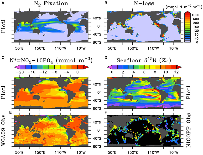
Figure 2. Preindustrial control (PIctl) annual vertically-integrated (A) N₂ fixation and (B) water column plus sedimentary N-loss. Comparison of upper ocean (0–300 m) N* and seafloor δ¹⁵N of PIctl (C,D) to (E) World Ocean Atlas 2009 (WOA09) (Garcia et al., 2010b) and (F) NICOPP database (Tesdal et al., 2013) observations. (B–D) Contours of minimum dissolved oxygen (10 mmol m⁻³) in the water column show where water column N-loss occurs.

Global mean δ¹⁵${\text{NO}}_3^{-}$ is determined by global rates and isotope effects of N₂ fixation, and water column and sedimentary N-loss (Brandes and Devol, 2002; Altabet, 2007). Sedimentary N-loss rates and its isotope effect represent the largest uncertainties for determining global mean δ¹⁵${\text{NO}}_3^{-}$ (Devries et al., 2013; Somes et al., 2013). Therefore, we took an empirical approach and chose the sedimentary N-loss fractionation factor (ε_SedNl = 6‰) within its estimated uncertainity range (1.5–13‰; Brandes and Devol, 1997; Lehmann et al., 2007; Granger et al., 2011; Dale et al., 2014) that sets deep ocean δ¹⁵${\text{NO}}_3^{-}$ near its observed ~5‰ value given the model predicted rates of N₂ fixation, water column N-loss, and sedimentary N-loss described above.

Last Glacial Maximum Model Configurations

Similar to Schmittner and Somes (2016) and guided by the Paleoclimate Model Intercomparison Project (PMIP3; Braconnot et al., 2012), we prescribe the LGM boundary conditions of the model: lower atmospheric concentrations of the greenhouse gases carbon dioxide, nitrous oxide, and methane, changes of Earth's orbit, and the increased area and height of ice sheets (Peltier, 2004). The ocean grid bathymetry and total ocean volume remains unchanged relative to the preindustrial simulation. However, effects of reduced sea level on sedimentary N-loss are accounted for by calculating a new sub-grid scale bathymetry scheme assuming a constant 120 m sea level reduction (Figure S1). This is different from SS16, who neglected sea level effect. The marine biogeochemistry equations are identical in the preindustrial and LGM simulations with parameters given in Table 1.

TABLE 1

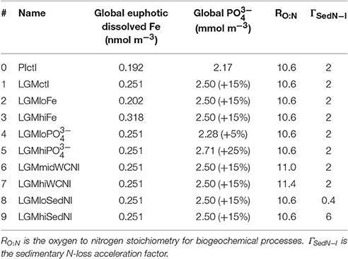
Table 1. Model configurations.

Wind stress anomalies (LGM minus preindustrial) are prescribed using monthly averages of 8 models that participated in the PMIP3 (Muglia and Schmittner, 2015) since the UVic model does not include an atmospheric general circulation component (Figure S3). This is different from SS16, who used pre-industrial wind stress. As shown by Muglia and Schmittner (2015), LGM wind stress anomalies increase the Atlantic Meridional Overturning Circulation (AMOC). We further deviate from SS16 by reducing moisture diffusivity in the 2D energy-moisture balance atmospheric model across the Southern Ocean by a factor of 2. Reduced meridional atmospheric moisture flux has been suggested as an important mechanism to influence glacial stratification and carbon storage in the Southern Ocean (Sigman et al., 2007), which weakens and shoals the AMOC in our model. The resulting AMOC is weaker (~9.9 Sv maximum) and shallower (by ~500 m as indicated by shoaling of the zero streamfunction line in Figures 1B,E from ~2,700 to ~2,200 m), similar to that of SS16 due to the compensating effects of wind stress and moisture diffusivity changes. The simulations were initialized with results from SS16 and run for over 8,000 years as they approached their quasi steady-state solution.

Atmospheric Fe Deposition

We account for increased atmospheric Fe deposition during the LGM (Figure 3). LGM and preindustrial dust flux estimates were obtained from Albani et al. (2014). We assumed a 3.5% Fe content in dust, and variable solubility was used from an atmospheric model that simulates the relation between modern iron flux and solubility of iron in dust (Luo et al., 2008). We applied their relationship to LGM and preindustrial dust fluxes, thereby obtaining surface soluble atmospheric Fe fluxes (Figure S4).

FIGURE 3

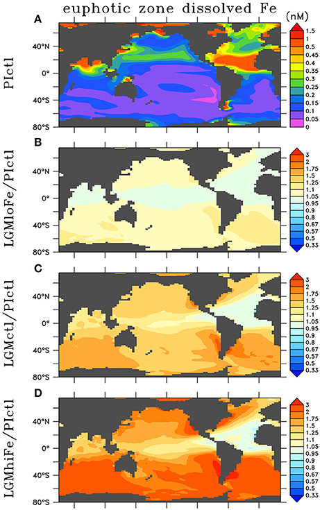
Figure 3. Annual euphotic zone dissolved iron in (A) preindustrial control (PIctl) and the ratio relative to preindustrial of the LGM simulations (B) LGMloFe, (C) LGMctl, and (D) LGMhiFe based on LGM atmospheric deposition estimates (Albani et al., 2014).

To predict the surface soluble atmospheric Fe fluxes effect on dissolved Fe concentrations in our model, we analyzed the global relationship between soluble atmospheric Fe flux (atmFeflx) and dissolved Fe (dFe) in the upper ocean from a different model that includes Fe as a prognostic tracer (Nickelsen et al., 2015). The relationship that yielded the highest correlation (R = 0.33) was a power law of the form dFe = A × (atmFeflx)^B where A = 6.3 × 10⁻⁴ and B = 0.24 (Figure S4). LGM dissolved Fe was calculated as dFe_LGM = (atmFeflx_LGM/atmFeflx_PI)^B× dFe_PI. This pragmatic approach is used due to high uncertainties associated with atmospheric dust deposition rates and Fe solubility, responsible for soluble Fe deposition estimates that differ by over an order of magnitude in different preindustrial global marine iron models (Tagliabue et al., 2016). In our LGM Fe sensitivity experiments, we changed the exponent B by the value ±0.2 from the LGM control value 0.25, which yields ± ~20% changes to global euphotic zone dissolved Fe concentrations (Table 1, Figure 3).

${\text{PO}}_4^{3-}$ Inventory

We test a hypothesis that the global ${\text{PO}}_4^{3-}$ inventory was larger during the LGM mainly due to reduced organic phosphorus burial on the exposed continental shelves from lower sea level (Broecker, 1982; Wallmann, 2010; Wallmann et al., 2016). Since the global oceanic ${\text{PO}}_4^{3-}$ inventory is conserved in each model simulation, we implement this hypothesis by imposing the estimated + ~15% increase in the global ${\text{PO}}_4^{3-}$ inventory from Wallmann et al. (2016) in LGMctl (Table 1). Model experiments #4 ${\text{LGMloPO}}_4^{3-}$ and #5 ${\text{LGMhiPO}}_4^{3-}$ probe its sensitivity to ±10% global ${\text{PO}}_4^{3-}$ change relative to LGMctl.

N-Loss Rates

We perform additional simulations to investigate how different water column and sedimentary N-loss rates affect LGM nitrogen cycling and δ¹⁵N distributions. In the model, water column N-loss can be increased pragmatically by increasing the elemental ratio of oxygen consumed per organic nitrogen remineralized (R_O:N, see Table 1). This leads to more oxygen loss, lower oxygen concentrations and larger ODZs in the model, thereby increasing water column N-loss. We interpret these simulations as water column N-loss sensitivity experiments rather than predictions of higher R_O:N stoichiometry, however noting that Devries and Deutsch (2014) suggest this ratio is higher in more stratified, nutrient depleted surface regimes that are more prevalent features in the LGM. Model experiment #6 (LGMmidWCNl) and #7 (LGMhiWCNl) assume R_O:N ratios of 11.0 and 11.4, respectively, compared to the standard value of 10.6 used in the preindustrial and LGM control simulations.

Sedimentary N-loss has been altered separately by changing its rate only on the subgrid-scale bathymetry scheme. We have applied an acceleration parameterization focused on narrow continental shelves in the upper 250 m to account for poorly resolved coastal processes (e.g., upwelling) that fuel sedimentary N-loss there (Figure S1). In the control simulations, applying an acceleration factor of 2 in this scheme increases sedimentary N-loss by 29 Tg N yr-1 (44%) in PIctl and 11 Tg N yr⁻¹ (29%) in LGMctl. LGM model experiments #8 LGMloSedNl and #9 LGMhiSedNl demonstrate the model sensitivity to this parameterization with lower and higher factors (Table 1), respectively, which altered global rates by ± ~40% relative to LGMctl (Table 2) in this sensitivity test. Note that since LGMloSedNl does not contain the sedimentary N-loss acceleration formulation, its factor is applied directly to the sedimentary N-loss rate on the subgrid-scale scheme. These N-loss sensitivity simulations were initialized with LGMctl and run for an additional 4,000 years.

TABLE 2

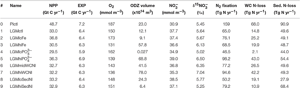
Table 2. Global biogeochemical model results.

LGM Model Results

In this section, we first provide a brief overview of the physical climate since the focus of this study is on marine biogeochemistry, noting that the physical climate (e.g., temperature and circulation) is identical for all LGM simulations. The subsequent subsection describes the LGMctl biogeochemistry relative to PIctl, followed by the LGM sensitivity experiments.

Physical Climate

The model reproduces major physical characteristics of the LGM climate, which are identical in all LGM simulations. Global average surface air temperature is 4.3°C colder in the LGMctl. The AMOC is shallower and weaker (9.9 Sv) compared to PIctl (17.1 Sv; Figure 1). Global mean Δ¹⁴C values are −165 and −225‰ in PIctl and LGMctl, respectively. Bottom waters in the LGMctl simulation are colder everywhere and saltier except for the eastern North Atlantic, where they are fresher compared with PIctl (Figure S5) due to the shoaling and weakening of the AMOC since Antarctic Bottom Water is fresher than North Atlantic Deep Water in the model. The simulated pattern of salinity changes indicates enhanced brine rejection from intensified sea ice formation in the Weddell Sea. The basin scale simulated changes in bottom water properties are qualitatively consistent with observations (Figure S5; Adkins et al., 2002; Insua et al., 2014). The simulated decrease of Δ¹⁴C below 2 km depth (−75‰, ~800 years radiocarbon age) is slightly older than a recent estimate of ~600 years based on sediment reconstructions (Sarnthein et al., 2013).

LGM Control Marine Biogeochemistry

In LGMctl, oxygen concentrations are higher above ~1,500 m and lower below (Figures 4A,B) relative to PIctl, which is consistent with O₂ reconstructions (Jaccard and Galbraith, 2012). The colder LGM climate enhances sea surface solubility of oxygen that is responsible for the upper ocean increase (Meissner et al., 2005). The combination of the more sluggish AMOC (Figure 1C) and increased sea ice cover, which reduce oxygen supply to the deep ocean, and enhanced atmospheric Fe deposition (Figure 3), which fuels organic matter export production that increases subsurface oxygen consumption, are the main factors responsible for the decreased deep ocean oxygen concentrations. On the global average, there is a 21.5% reduction of the global O₂ inventory (Table 2). This is similar to the 20.8% reduction resulting from SS16's best δ¹⁵N simulation, who attribute ~7% of this decrease to physics and ~14% to changes in Fe fertilization.

FIGURE 4

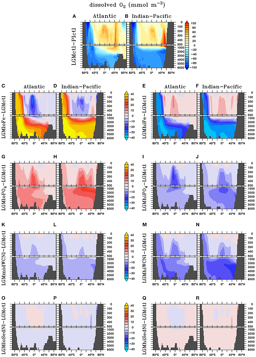
Figure 4. Zonal dissolved oxygen differences in the Atlantic and Indian-Pacific Oceans, respectively, of (A,B) Last glacial Maximum control (LGMctl) minus preindustrial control (PIctl) and the Last Glacial Maximum simulations minus LGM control: (C,D) LGMloFe, (E,F) LGMhiFe, (G,H) ${\text{LGMloPO}}_4^{3-}$, (I,J) ${\text{LGMhiPO}}_4^{3-}$, (K,L) LGMmidWCNl, (M,N) LGMhiWCNl, (O,P) LGMloSedNl, and (Q,R) LGMhiSedNl.

Higher O₂ concentrations in the upper ocean reduce the volume of ODZs by 47% and water column N-loss by 78% (Figures 5B, 6). The difference in the reduction of ODZ volume compared to water column N-loss rate occurs due to the emergence of a ODZ in the deep (1,000–2,000 m) subarctic Pacific that accounts for 10% of total water column N-loss in LGMctl, which cannot be excluded because trace metal proxies at bottom waters in these locations indicate less oxygen during the LGM (Jaccard and Galbraith, 2012). Here, OM remineralization rates that drive water column N-loss are lower than in the shallower tropical ocean, which results in less water column N-loss per volume of ODZ waters. In combination with decreased sedimentary N-loss by 55% due to exposed continental shelves from lower sea level in LGMctl (e.g., Bering Sea Shelf, North Atlantic; Figure 5B), total N-loss decreases by 59% (Table 2, Figure 6). However, note that some regions at mid-latitudes in the Southern Ocean, North Pacific, and North Atlantic show increases in sedimentary N-loss due enhanced atmospheric Fe deposition fueling additional export production (Figure 5B). Although reduced total N-loss occurs primarily in the upper ocean, the resulting increased ${\text{NO}}_3^{-}$ accumulates in the deep ocean due to enhanced POM export in the Southern Ocean that remineralizes and remains for longer in the older, more sluggish Antarctic Bottom Waters in LGMctl.

FIGURE 5

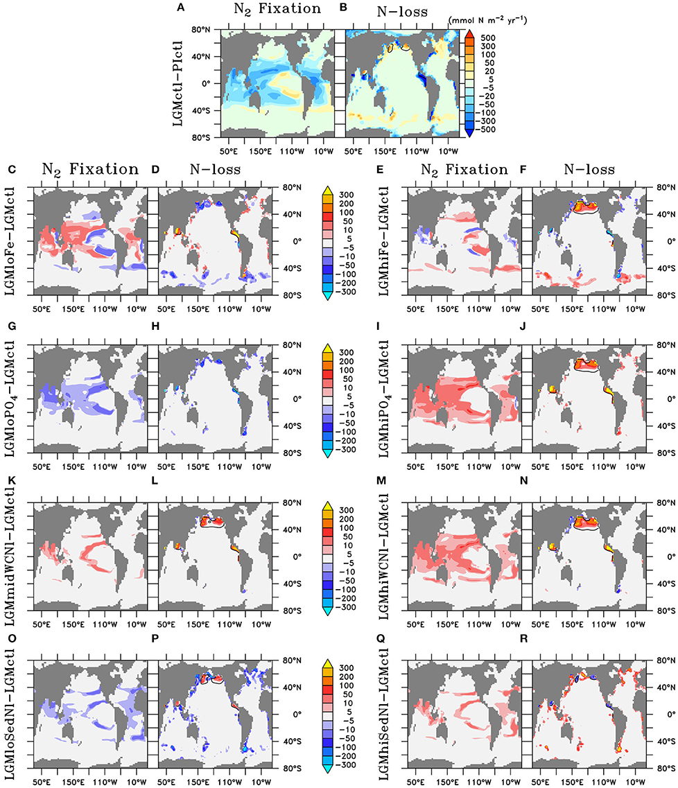
Figure 5. Vertically-integrated differences of N₂ fixation and total N-loss, respectively, of (A,B) Last Glacial Maximum control (LGMctl) minus preindustrial control (PIctl) and the Last Glacial Maximum simulations minus LGM control: (C,D) LGMloFe, (E,F) LGMhiFe, (G,H) ${\text{LGMloPO}}_4^{3-}$, (I,J) ${\text{LGMhiPO}}_4^{3-}$, (K,L) LGMmidWCNl, (M,N) LGMhiWCNl, (O,P) LGMloSedNl, and (Q,R) LGMhiSedNl. Contours of minimum dissolved oxygen (10 mmol m⁻³) in the water column show where water column N-loss occurs.

FIGURE 6

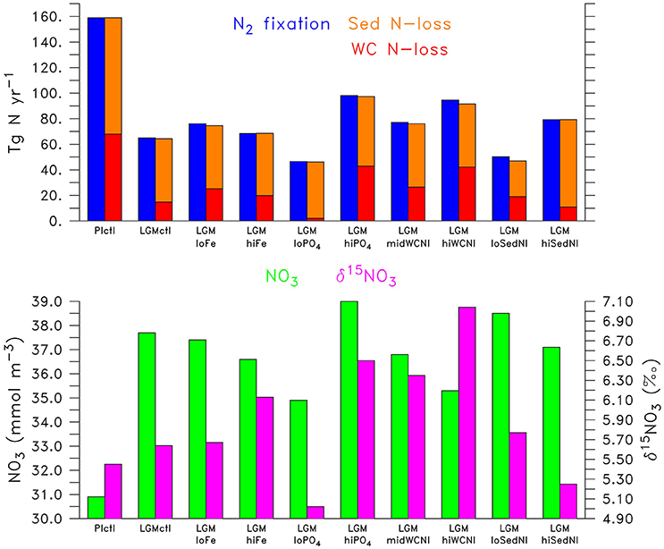
Figure 6. (Top) Global N₂ fixation (left blue bar), water column N-loss (right red bar), and sedimentary N-loss (right orange bar) for the simulations. (Bottom) Global ${\text{NO}}_3^{-}$ (left green bar) and global δ¹⁵${\text{NO}}_3^{-}$ (right magenta bar) for the simulations.

N₂ fixation decreases in the LGMctl simulation by 59% mainly in response to the reduction in N-loss when approaching the steady-state solution (Figures 5, 6). Only the oligotrophic eastern tropical Pacific and southern boundary of the southern subtropical gyres show subtle increases of N₂ fixation due to enhanced atmospheric Fe deposition (Figure 5A). In the LGMctl model, global N₂ fixation is not sensitive to increased Fe deposition because glacial estimates of increased Fe deposition applied here (Albani et al., 2014) primarily occur at high latitudes where diazotrophs are limited by temperature. However, the combined effects of the changes in sources and sinks result in a significantly increased global ${\text{NO}}_3^{-}$ inventory (+22%). Note that DOP utilization by diazotrophs does not play a significant role stimulating N₂ fixation in LGMctl because nitrogen limitation is reduced due to the larger ${\text{NO}}_3^{-}$ inventory and thus ordinary phytoplankton outcompete diazotrophs for the majority of DOP consumption.

Atmospheric Fe Deposition Sensitivity

Atmospheric Fe deposition was increased during the LGM compared to pre-industrial times, which has a large fertilizing effect on organic matter production in the HNLC regions of the Southern Ocean, subarctic North Pacific, and equatorial eastern Pacific in the model. Additional ${\text{NO}}_3^{-}$ is thus consumed at the surface and stored in the deep ocean (Figures 7A,B), where it can remain for millennia.

FIGURE 7

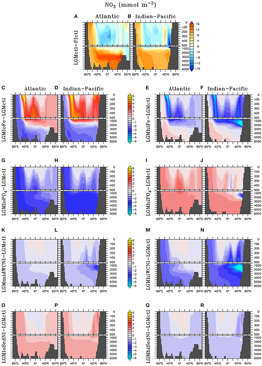
Figure 7. Zonal dissolved nitrate (${\text{NO}}_3^{-}$) differences in the Atlantic and Indian-Pacific Oceans, respectively, of (A,B) Last glacial Maximum control (LGMctl) minus preindustrial control (PIctl) and the Last Glacial Maximum simulations minus LGM control: (C,D) LGMloFe, (E,F) LGMhiFe, (G,H) ${\text{LGMloPO}}_4^{3-}$, (I,J) ${\text{LGMhiPO}}_4^{3-}$, (K,L) LGMmidWCNl, (M,N) LGMhiWCNl, (O,P) LGMloSedNl, and (Q,R) LGMhiSedNl.

Enhanced export production at high latitudes reduces the amount of preformed surface ${\text{NO}}_3^{-}$ in Subantarctic Mode Waters that flow to the tropics (Figures 7C–F). This reduces tropical productivity, volume of tropical ODZs and global water column N-loss in LGMhiFe relative to LGMloFe (Table 2). Intermediate waters (~1,000–2,000 m) in the subarctic North Pacific are near the threshold of suboxia in simulation LGMctl. Those suboxic regions intensify when enhanced atmospheric Fe deposition in LGMhiFe stimulates additional organic matter remineralization (Figure 4F), which enhances water column N-loss (Figure 5F).

Only minor increases to N₂ fixation are stimulated by enhanced atmospheric Fe deposition in the model (Figure 5E). This is most pronounced in two zones in the southern hemisphere that are largely Fe limited in the preindustrial ocean: the eastern tropical Pacific and a zonal band across the edge of the southern subtropical gyres. Since diazotrophs prefer warm oligotrophic N-limited surface conditions, they grow outside the cold, high surface ${\text{NO}}_3^{-}$ waters of the eastern equatorial Pacific upwelling region. Although, not typically thought to occur outside the tropics, the strong atmospheric Fe deposition originating around Patagonia (Figure 3) is sufficient to stimulate N₂ fixation in our model. However, on the global average, these areas of additional N₂ fixation are much smaller than areas in which N₂ fixation decreased in model LGMctl relative to PIctl due to reduced N-loss (Figure 5A).

Water column δ¹⁵${\text{NO}}_3^{-}$ is strongly influenced by nitrogen cycling changes in response to enhanced atmospheric Fe deposition (Figure 8). Enhanced (reduced) surface ${\text{NO}}_3^{-}$ utilization increases (decreases) surface δ¹⁵${\text{NO}}_3^{-}$ in the Southern Ocean and Subarctic Pacific in LGMhiFe (LGMloFe). The minor increase (decrease) to N₂ fixation rates in the southern tropics and subtropics in LGMhiFe (LGMloFe) substantially decreases (increases) δ¹⁵${\text{NO}}_3^{-}$. This large isotopic signal occurs because these systems switch from being driven by high ${\text{NO}}_3^{-}$ utilization, which causes extremely ¹⁵N-enriched surface ${\text{NO}}_3^{-}$, to a N₂ fixation isotopic regime that introduces ¹⁵N-depleted nitrogen to the surface ocean. This model prediction suggests that all relevant processes should be considered when interpreting δ¹⁵N and the change to the isotopic signal may not be linearly representative of the rate change to one specific nitrogen cycling process alone.

FIGURE 8

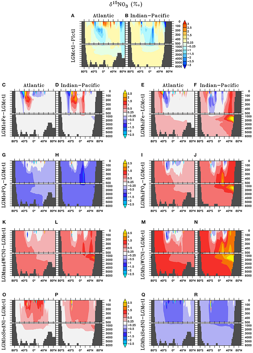
Figure 8. Zonal dissolved δ¹⁵N of nitrate (δ¹⁵${\text{NO}}_3^{-}$) differences in the Atlantic and Indian-Pacific Oceans, respectively, of (A,B) Last glacial Maximum control (LGMctl) minus preindustrial control (PIctl) and the Last Glacial Maximum simulations minus LGM control: (C,D) LGMloFe, (E,F) LGMhiFe, (G,H) ${\text{LGMloPO}}_4^{3-}$, (I,J) ${\text{LGMhiPO}}_4^{3-}$, (K,L) LGMmidWCNl, (M,N) LGMhiWCNl, (O,P) LGMloSedNl, and (Q,R) LGMhiSedNl.

Global ${\text{PO}}_4^{3-}$ Inventory Sensitivity

The model simulations testing a hypothesized increase to the global ${\text{PO}}_4^{3-}$ inventory predict larger ${\text{NO}}_3^{-}$ inventories due to enhanced N₂ fixation (Table 2, Figures 6, 7G–J). ${\text{PO}}_4^{3-}$ is the major limiting macronutrient for N₂-fixing diazotrophs. Although N-loss is reduced during the LGM, N-limitation still persists, leaving the tropical and subtropical ocean mostly N limited. Therefore, increased ${\text{PO}}_4^{3-}$ stimulates additional growth of diazotrophs via N₂ fixation that is most pronounced in the tropical ocean. The additional organic matter production via enhanced N₂ fixation and remineralization at depth stimulates additional water column N-loss, which balances the enhanced N₂ fixation at a new steady-state with a larger global ${\text{NO}}_3^{-}$ (Figure 6) and reduced O₂ inventory (Figures 4I,J). A 10% increase in the ${\text{PO}}_4^{3-}$ inventory thus causes an 8% increase in the ${\text{NO}}_3^{-}$ inventory (LGMctl-${\text{LGMloPO}}_4^{3-}$). However, a further 10% increase in the ${\text{PO}}_4^{3-}$ inventory (${\text{LGMhiPO}}_4^{3-}$-LGMctl) leads to diminishing returns in terms of ${\text{NO}}_3^{-}$ (4%) due to the further expansion of ODZs and N-loss. The additional N₂ fixation decreases surface δ¹⁵${\text{NO}}_3^{-}$ in the tropics and subtropics, whereas the additional water column N-loss increases subsurface δ¹⁵${\text{NO}}_3^{-}$ in the Indian and Pacific (Figures 8I,J).

N-Loss Sensitivity

The water column N-loss sensitivity simulations alter rates by increasing oxygen consumption during organic matter remineralization, thereby decreasing subsurface oxygen concentrations (Figures 4K–N). Note that these simulations do not change the large-scale pattern of higher oxygen in the upper ocean and lower oxygen in the deep ocean that is supported by observational constraints (Jaccard and Galbraith, 2012), but only reduces the magnitude of this qualitative trend in the deep ocean. Enhanced water column N-loss in the expanded ODZs in LGMmidWCNl and LGMhiWCNl reduces ${\text{NO}}_3^{-}$ in the eastern tropical Pacific, North Indian, and subarctic Pacific (Figures 7K–N). This significantly increases subsurface δ¹⁵${\text{NO}}_3^{-}$ since water column N-loss has a strong isotope effect (Figures 8K–N). Even though this signal is generated in the ODZs of the tropical ocean and subarctic Pacific, it eventually reaches the Southern Ocean and has a global impact (Figures 8K–N).

Sedimentary N-loss has lower local rates that are spread throughout all ocean basins so its signal is more distributed through the global ocean compared to vertically-integrated water column N-loss. Enhanced (reduced) rates in LGMhiSedNl (LGMloSedNl) decreases (increases) global ${\text{NO}}_3^{-}$ (Figures 7O–R). Since sedimentary N-loss has a relatively small isotope effect, its main isotopic signal is an indirect one by stimulating additional (less) N₂ fixation to balance additional (less) sedimentary N-loss in LGMhiSedNl (LGMloSedNl). This decreases (increases) surface δ¹⁵${\text{NO}}_3^{-}$ most notably in the tropical and subtropical ocean basins (Figures 8O–R).

Nitrogen Isotope Model-Data Analysis

Modeled nitrogen isotopes are compared to 61 datapoints from the recent synthesis of reconstructions from the Nitrogen Cycling in the Oceans Past and Present (NICOPP) group (Galbraith et al., 2013) for which LGM—Late Holocene differences are available. These data, based on bulk organic nitrogen measurements, were corrected for a diagenetic effect according to Robinson et al. (2012), who examined over 100 locations and found a significant correlation with water depth (~1‰/km), while noting that oxygen exposure time is likely the main driver. We use the five additional foraminifera and diatom bound measurements included in Schmittner and Somes (2016), plus 6 more from recent studies in the subarctic Pacific and central equatorial Pacific (Ren et al., 2015; Costa et al., 2016), all of which were not corrected for diagenesis. Although combining different forms of δ¹⁵N records creates uncertainty, excluding the diatom and foraminifera bound measurements does not affect which simulations performed best in terms of the statistical model-data metrics so we include them into the main analysis to improve spatial coverage.

Overall, δ¹⁵N records from LGM sediments document lower values in modern ODZs such as the eastern tropical Pacific and Arabian Sea indicating less water column N-loss, higher values in the western tropics of the North Pacific and North Atlantic indicating less N₂ fixation, and higher values in high latitude HNLC regions (i.e., Southern Ocean, western subarctic Pacific) indicating enhanced surface ${\text{NO}}_3^{-}$ utilization (Figures 9–11). These sedimentary δ¹⁵N records are compared to the δ¹⁵N values of sinking particulate organic nitrogen (PON) in bottom waters above the seafloor, which we refer to as sedimentary δ¹⁵N in the model below. Our model does not account for terrestrial sources of δ¹⁵N, which can influence records near the continental margin and potentially contribute to model-data misfits. Therefore, we focus our analysis and discussion on regions that are strongly influenced by marine nitrogen cycling processes, but note that all data points are included in the model-data statistical metrics.

FIGURE 9

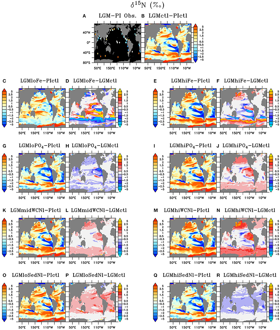
Figure 9. Sedimentary δ¹⁵N of (A) LGM minus preindustrial observations and (B) Last Glacial Maximum control (LGMctl) minus preindustrial control (PIctl). Sedimentary δ¹⁵N differences of the Last Glacial Maximum simulations: (C,D) LGMloFe, (E,F) LGMhiFe, (G,H) ${\text{LGMloPO}}_4^{3-}$, (I,J) ${\text{LGMhiPO}}_4^{3-}$, (K,L) LGMmidWCNl, (M,N) LGMhiWCNl, (O,P) LGMloSedNl, and (Q,R) LGMhiSedNl minus PIctl and minus LGMctl are shown, respectively.

FIGURE 10

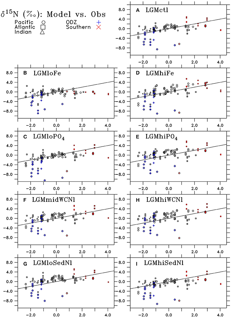
Figure 10. Comparison of LGM minus PI changes in sedimentary δ¹⁵N from observations (horizontal axis) and model results (vertical axis) of (A) LGMctl, (B) LGMloFe, (C) ${\text{LGMloPO}}_4^{3-}$, (D) LGMhiFe, (E) ${\text{LGMhiPO}}_4^{3-}$, (F) LGMmidWCNl, (G) LGMloSedNl, (H) LGMhiWCNl, and (I) LGMhiSedNl. Locations in the Pacific, Atlantic, and Indian Oceans are shown as circles, squares, and triangles, respectively. Locations in oxygen deficient zones (ODZ; minimum O₂ < 10 mmol m⁻³) are shown as blue crosses and Southern Ocean (south of 40°S) are red Xs. The black line indicates a “perfect” representation of observations.

FIGURE 11

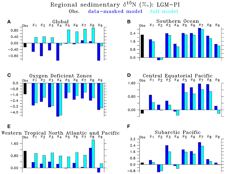
Figure 11. Regional Last Glacial Maximum minus Preindustrial δ¹⁵N differences of LGM model simulations (#1) LGMctl, (#2) LGMloFe, (#3) LGMhiFe, (#4) ${\text{LGMloPO}}_4^{3-}$, (#5) ${\text{LGMhiPO}}_4^{3-}$, (#6) LGMmidWCNl, (#7) LGMhiWCNl, (#8) LGMloSedNl, (#9) LGMhiSedNl in the (A) global ocean, (B) Southern Ocean (<40°S), (C) oxygen deficient zones (minimum O₂ <10 mmol m⁻³), (D) Central Equatorial Pacific (170°W–130°W, 5°N–5°S), (E) Western Tropical North Atlantic and Pacific (0–25°N, western 50° of Atlantic and Pacific basins), and (F) Subarctic Pacific (40–65°N). “Data-masked” model (dark blue left bar) only includes locations where data exist, whereas the “full” model (light blue right bar) averages over the entire region.

LGM Control Simulation

Model simulation LGMctl, which includes enhanced atmospheric Fe deposition and assumes a +15% increase to the global ${\text{PO}}_4^{3-}$ inventory, reproduces the major trends in the LGM reconstructions (R = 0.45, Table 3; Figures 9–11). It reproduces the largest increase in δ¹⁵N in the Southern Ocean with respect to preindustrial values (Figure 11B) and the smaller increase in the subarctic Pacific HNLC region (Figure 11F). However, it predicts a slight increase (+0.7‰) to the Central Equatorial Pacific, where the data show a minor decrease (−0.2‰). The largest model-data mismatch exists in the Eastern Tropical North Pacific ODZ, where the predicted decrease of δ¹⁵N is too strong relative to observations (Figure 11C).

TABLE 3

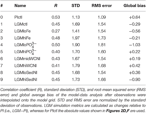
Table 3. δ¹⁵N model-data statistical metrics.

The change to global δ¹⁵${\text{NO}}_3^{-}$ (Table 2) and sedimentary δ¹⁵N (Figure 11A) in LGMctl relative to PIctl is small compared to the change of the ratio of sedimentary to water column N-loss, which in part determines global δ¹⁵${\text{NO}}_3^{-}$ (Somes et al., 2013). This relatively small δ¹⁵${\text{NO}}_3^{-}$ change is due to the dilution effect in N-loss zones (Deutsch et al., 2004), which increases the isotope effect of water column N-loss (per mole N removed) in LGMctl relative to PIctl as ${\text{NO}}_3^{-}$ utilization decreases in the smaller ODZs. This effect decreases the isotopic signature of δ¹⁵N removed by water column N-loss from −5.1‰ in PIctl to −10.3‰ in LGMctl, thereby increasing its isotope effect by 5.2‰. This also occurs to a lesser degree in bottom waters where sedimentary N-loss occurs increasing its isotope effect by 1.1‰. Therefore, additional N₂ fixation and thus a higher ratio of sedimentary to water column N-loss is required to balance the increased isotope effect from N-loss on global δ¹⁵${\text{NO}}_3^{-}$ in the LGMctl steady-state solution compared to PIctl.

The processes that lead to slightly higher deep ocean δ¹⁵${\text{NO}}_3^{-}$ in LGMctl are mainly controlled at high latitudes. In the North Atlantic, reduced N₂ fixation elevates surface δ¹⁵${\text{NO}}_3^{-}$ that eventually subducts in the Atlantic meridional overturning circulation and increases deep ocean δ¹⁵${\text{NO}}_3^{-}$ (Figure 8A). In the Southern Ocean, enhanced atmospheric Fe deposition increases ${\text{NO}}_3^{-}$ utilization and the isotopic signature of sinking particulate organic nitrogen (PON) that remineralizes at depth (Figures 8A,B, 9B). The emergence of a small ODZ in the deep (1,000–2,000 m) subarctic Pacific (Figure 5B), which accounts for 10% of total water column N-loss in LGMctl, contributes to elevated deep ocean δ¹⁵${\text{NO}}_3^{-}$ as well. Since most of the increased ${\text{NO}}_3^{-}$ inventory in LGMctl accumulates in these old, sluggish deep waters, our modeling suggests that high latitude process also play a role determining global mean δ¹⁵${\text{NO}}_3^{-}$, not only N₂ fixation and water column N-loss in the tropics.

Atmospheric Fe Deposition Sensitivity

Lower atmospheric Fe deposition in LGMloFe compared to LGMctl reduces ${\text{NO}}_3^{-}$ utilization and sedimentary δ¹⁵N in HNLC regions (Figures 9C,D), where the fit with observations deteriorates (Figures 10B,11B). The better agreement of the magnitude of the increase in δ¹⁵N in LGMctl in the Southern Ocean and Subarctic Pacific supports LGMctl's assumption for increased Fe deposition during the LGM in those regions. In fact, LGMctl's increase in ${\text{NO}}_3^{-}$ utilization may be underestimated in the Southern Ocean, where simulation LGMhiFe agrees better with the observations (Figure 11B).

In the Central Equatorial Pacific, which is on the western border of the eastern Pacific HNLC region, both LGM Fe sensitivity simulations reproduce the observations better than LGMctl (Figure 11D), but for different reasons. In LGMloFe, the small increase to atmospheric Fe deposition was insufficient to increase ${\text{NO}}_3^{-}$ utilization and hence sedimentary δ¹⁵N in this region. In our high-end simulation for atmospheric Fe deposition (LGMhiFe), enhanced N₂ fixation introducing additional ¹⁵N-depleted nitrogen reduces the overestimated model bias of LGMctl. Until more observations in and around the central and eastern tropical Pacific HNLC become available, it will remain difficult to evaluate whether relatively low ${\text{NO}}_3^{-}$ utilization or increased N₂ fixation was the most important process driving the observed decreased LGM δ¹⁵N trend.

Our sensitivity model experiments in the Southern Hemisphere show a balance between lower δ¹⁵N due to enhanced N₂ fixation in the subtropics and higher δ¹⁵N from enhanced surface ${\text{NO}}_3^{-}$ utilization toward high latitudes. Our model predicts that increased Fe could stimulate additional N₂ fixation at the poleward edge of the southern subtropics as far south as ~40°S, which counteracts with the isotope effect of enhanced ${\text{NO}}_3^{-}$ utilization that increases δ¹⁵N at higher latitudes (Figures 8C–F, 9C–F). As ${\text{NO}}_3^{-}$ decreases with enhanced atmospheric Fe deposition, the additional ¹⁵N-depleted nitrogen via N₂ fixation contributes to a larger fraction of total sinking PON, which prevents a higher δ¹⁵N increase in LGMhiFe compared to the δ¹⁵N decrease in LGMloFe (Figure 11B). The absence of open ocean δ¹⁵N observations in the tropical and subtropical southern hemisphere makes it uncertain to validate this increase to N₂ fixation there.

Global ${\text{PO}}_4^{3-}$ Inventory Sensitivity

In the model, a larger global ${\text{PO}}_4^{3-}$ inventory stimulates increases to N₂ fixation, water column N-loss, and the global ${\text{NO}}_3^{-}$ inventory (Figure 6). This results in increased sedimentary δ¹⁵N near ODZs and decreased δ¹⁵N outside of them in the more oligotrophic ocean where additional N₂ fixation occurs (Figure 9J). The magnitude of change to δ¹⁵N in the model (Figure 10) is relatively small because N₂ fixation and water column N-loss have counteracting nitrogen isotopic effects. Since these processes occur within close spatial proximity in the tropics, the input of ¹⁵N-depleted nitrogen via fixation roughly compensates the extra ¹⁵N-enriched ${\text{NO}}_3^{-}$ via enhanced water column N-loss rates, preventing a larger change to the large scale δ¹⁵N signal (Figures 9G–J).

Despite large changes to the global rates of these processes, changes to simulated δ¹⁵N at the location of observations only moderately affect the model-data statistical metrics (Table 3, Figure 10). The higher water column N-loss in ${\text{LGMhiPO}}_4^{3-}$ better reproduces δ¹⁵N in tropical ODZs (Figure 11C). However, the additional water column N-loss in the subarctic Pacific overestimates δ¹⁵N in that region. The model experiment ${\text{LGMloPO}}_4^{3-}$ performs best in the Central Equatorial Pacific (Figure 11E), which suggests that the additional ${\text{PO}}_4^{3-}$ stimulates too much N₂ fixation there in simulations LGMctl and ${\text{LGMhiPO}}_4^{3-}$.

N-Loss Rate Sensitivity

Since one of the main model deficiencies in LGMctl is underestimated δ¹⁵N in ODZs (Figures 10, 11C), we performed sensitivity simulations with higher water column N-loss rates (#7 LGMmidWCNl and #8 LGMhiWCNl). Imposing moderately higher water column N-loss rates increases δ¹⁵N in existing ODZ zones in the Eastern Pacific and North Indian Ocean and reduces the model-data mismatch in those regions (Figure 11C). However, the enhanced water column N-loss rates also increases δ¹⁵N in the Central Equatorial Pacific and Subarctic Pacific, causing those regions to overestimate δ¹⁵N compared to the observations, demonstrating how water column N-loss influences δ¹⁵N across the entire tropical Pacific and beyond (Figures 8K–N, 9K–N,P).

Higher water column N-loss rates increase global δ¹⁵${\text{NO}}_3^{-}$ (Figures 8K–N), but this does not impact sedimentary δ¹⁵N everywhere equally (Figures 9K–N). Effects are largest in regions with upwelling of the increased deep ocean δ¹⁵${\text{NO}}_3^{-}$, e.g., tropical Pacific, subarctic North Pacific, and Southern Ocean. Our simulations suggest that if a significant increase in global δ¹⁵${\text{NO}}_3^{-}$ occurred during the LGM, this could significantly impact δ¹⁵N across the Southern Ocean, which are typically interpreted as changes to surface ${\text{NO}}_3^{-}$ utilization alone. Given the sparsity of the global dataset, we cannot exclude a significant increase in global δ¹⁵${\text{NO}}_3^{-}$ during the LGM because its large-scale impact affects sedimentary δ¹⁵N in regions that already have an increased δ¹⁵N trend relative to PI (e.g., Southern Ocean, subarctic Pacific). The model results suggest that the distribution of existing sites is such that calculating a global average from those sites alone would underestimate the true global mean by ~0.8‰ (Figure 11). In fact, those models that fit the mean in the data best (#6, 8) indicate a ~0.8‰ higher global mean in the LGM compared to PI.

Sedimentary N-loss has a weak isotope effect that does not play a prominent direct role determining δ¹⁵N patterns in the model. Only areas directly above continental shelves with high sedimentary N-loss (e.g., Bering Sea) rates show a notable δ¹⁵N decrease due to its direct impact (Figure 9B). Its small effect on the δ¹⁵N makes it a difficult process to isotopically constrain, which creates high uncertainty on N cycling and inventory since it is the largest N-loss process in the global ocean.

The sensitivity simulations testing changes to sedimentary N-loss rates suggest that its most important isotope effect is an indirect one by stimulating changes to N₂ fixation. N₂ fixation rates are sensitive to N-loss because it enhances N-limitation, which in large part determines diazotroph's ecological niche. In LGMloSedNl, the reduced N₂ fixation in response to sedimentary N-loss increased δ¹⁵N in the tropics and subtropics, which reproduced observations better in the western Tropical North Atlantic and Pacific (Figure 11E), but worse in Central Equatorial Pacific (Figure 11D) compared to LGMctl.

Discussion

LGM Model Best Estimates and Uncertainty Ranges

Most LGM model simulations discussed here have similar global δ¹⁵N metrics. In general, the sensitivity experiments performed better in some regions but worse in others compared to LGMctl. Therefore, based on these objective global statistical metrics alone, one might conclude that most of our LGM models are similarly consistent with the observations. The only obvious exception is LGMloFe, which has a lower correlation coefficient than the other models, suggesting that enhanced iron fertilization played a crucial role in the glacial nitrogen cycle and its isotopic pattern, consistent with SS16's conclusions.

The simulations that perform among the best with both correlation coefficient (i.e., R > 0.44) and RMS error (i.e., error <1.55) metrics are LGMctl, LGMmidWCNl, and LGMloSedNl that largely determine our uncertainty ranges. However, some of the simulations perform better in regions that are representative of certain processes, which is also considered and discussed below. Overall, the model simulations struggle the most where the observations show small LGM−PI differences between ±1.5‰, whereas the stronger δ¹⁵N trends in ODZs and the Southern Ocean are better reproduced (Figure 10).

One of the main model biases in LGMctl is the too low δ¹⁵N in ODZs, presumably due to underestimated water column N-loss. The sensitivity simulations that assume higher water column N-loss reproduce those observations more closely. LGMhiWCNl, which predicts a 35% decrease in water column N-loss relative to PIctl, performs best in tropical ODZs but overestimates δ¹⁵N in the subarctic Pacific where water column N-loss also occurs in that simulation. The best simulation from SS16 that reproduces tropical ODZ slightly better predicts only a 17% decrease in water column N-loss. Therefore, we choose its global water column N-loss rate (57 Tg N yr⁻¹) as our high-end estimate with our next best performing simulation in ODZs (LGMmidWCNl: 26 Tg N yr⁻¹) as our low-end estimate, which yields a 17–62% decrease relative to PIctl.

Sedimentary N-loss is more difficult to constrain given its weak isotope effect. Our model predicts a lower global rate since sea level was reduced during the LGM. Since the sensitivity simulation LGMloSedNl results in improved model-data statistical metrics compared to LGMhiSedNl (Table 3, Figure 10), we use that simulations as our low-end range, with a value between LGMctl and LGMhiSedNl as our high-end estimate. This yields a 35–69% reduction of sedimentary N-loss during the LGMctl relative to PIctl.

The limited LGM observations interpreted as constraints on N₂ fixation are all located in the western tropical North Pacific and Atlantic. Our LGMctl model predicts reduced N₂ fixation in these regions relative to PIctl, in general agreement with previous interpretations (Ren et al., 2009, 2012). This occurs in the model in response to lower N-loss rates, which decrease the ecological nice for diazotrophy during the LGM relative to PI by reducing N-limitation. However, model LGMctl predicts an increase of N₂ fixation in the tropical and subtropical southern hemisphere due to enhanced atmospheric Fe deposition. Unfortunately no observational constraints exist in these Fe-limited regions in the southern hemisphere, where N₂ fixation has been hypothesized to occur increase during the LGM (Falkowski, 1997).

The most important sensitivity for global ${\text{NO}}_3^{-}$ in our model is the assumption about changes to global ${\text{PO}}_4^{3-}$, which fuels additional N₂ fixation that increases global ${\text{NO}}_3^{-}$. The model simulation with a low increase to ${\text{PO}}_4^{3-}$ (${\text{LGMloPO}}_4^{3-}$) did not stimulate enough productivity to maintain sufficient water column N-loss to reproduce δ¹⁵N observations in ODZs, whereas simulations with higher global ${\text{PO}}_4^{3-}$ performed better with respect to data there. However, many circulation and biogeochemical processes determine the size of ODZs so it remains difficult to confidently conclude that increased ${\text{PO}}_4^{3-}$ was likely the reason for maintaining ODZs in the LGM, but it remains a possibility that cannot be excluded here. In the Central Equatorial Pacific, ${\text{LGMloPO}}_4^{3-}$ performed best due to its lower N₂ fixation rates (Figure 11D), which suggests that the additional ${\text{PO}}_4^{3-}$ stimulated too much N₂ fixation there when a higher ${\text{PO}}_4^{3-}$ inventory was assumed.

The best performing model sensitivity simulations predict a large range in changes to the global ${\text{NO}}_3^{-}$ inventory (13–22%), which is most sensitive to assumptions for global ${\text{PO}}_4^{3-}$ inventory that has high uncertainties. If some unresolved physical process, e.g., increased diapycnal mixing (Schmittner et al., 2015), would be responsible for the δ¹⁵N bias in ODZs, this could decrease global ${\text{NO}}_3^{-}$ similarly to the LGMhiWCNl sensitivity simulation (i.e., +27 Tg N yr⁻¹ water column N-loss caused −2.2 mmol m⁻³ global ${\text{NO}}_3^{-}$). Applying this idealized linear relationship with our high-end estimate for water column N-loss reduction (57 Tg N yr⁻¹) to LGMctl would reduce its global ${\text{NO}}_3^{-}$ increase approximately in half because it underestimates water column N-loss. Thus, for our low-end uncertainty range for global ${\text{NO}}_3^{-}$, we apply this relative decrease to our simulation with lowest ${\text{PO}}_4^{3-}$ that predicts a +13% global ${\text{NO}}_3^{-}$ increase relative to PIctl, which yields a low-end increase of global ${\text{NO}}_3^{-}$ of ~6.5% based on our sensitivity simulations performed in this study.

Comparison with Previous Studies

Our model simulations produce lower oxygen levels in the glacial deep ocean below ~1,500 m compared to preindustrial (Figure 4) due to a combination of a weaker Atlantic meridional overturning circulation (Figure 1), which reduces deep ocean ventilation, and enhanced atmospheric Fe deposition over the Southern Ocean (Figure 2), which consumes oxygen during additional organic matter respiration. This large-scale model feature is consistent with proxy reconstructions (Jaccard and Galbraith, 2012). Since atmospheric Fe deposition was mainly increased over the Southern Ocean, enhanced export production stores more nutrients in Antarctic Bottom Water that fills the deep ocean. This causes less preformed nutrients transport to the tropics via Subantarctic Mode Waters, thereby reducing productivity and water column N-loss there, generally consistent with the scenario suggested by Costa et al. (2016).

The glacial upper ocean, on the other hand, was better oxygenated due to enhanced solubility from colder sea surface waters, which reduces the volume of oxygen deficient zones relative to preindustrial. The reduced oxygen deficient zones and exposed continental shelves due to lower sea level decreases water column and sedimentary N-loss in our model by 17–69% and 35–69%, respectively. Our uncertainty range agrees with Galbraith et al. (2013), although noting they examine the period between 15,000 and 8,000 years ago when the strongest deglacial changes occur.

Our simulations suggest that the ratio of sedimentary to water column total N-loss was higher in the LGM assuming no change to global δ¹⁵${\text{NO}}_3^{-}$, in contrast to Galbraith et al. (2013) who suggest a constant ratio. This occurs in our model due to the dilution effect (Deutsch et al., 2004), which decreases the apparent isotope effect of N-loss (per mole N removed) as ${\text{NO}}_3^{-}$ utilization increases in N-loss zones. Since in LGMctl N-loss rates were smaller due to diminished upper ocean ODZs and continental shelves, the dilution effect also decreased, thereby increasing the isotope effect of water column and sedimentary N-loss by 5.2 and 1.1‰, respectively, relative to PIctl. Therefore, additional N₂ fixation stimulated by sedimentary N-loss would be required to balance global δ¹⁵${\text{NO}}_3^{-}$ assuming an oceanic N isotope budget in equilibrium. However, the observed LGM-PI δ¹⁵N decrease in ODZs do not support such a large decrease of water column N-loss (Figure 11C). This leads to the possibility that global δ¹⁵${\text{NO}}_3^{-}$ was increased during the LGM, which we suggest cannot be excluded with the current sparsity of observations because the true model global sedimentary δ¹⁵N average (“full model” in Figure 11A) is not always consistent with limited locations where observations exist (“data-masked model” in Figure 11A). Our simulations suggest some of this potential global δ¹⁵${\text{NO}}_3^{-}$ increase would accumulate in the Southern Ocean (Figures 8K,L) and be partially responsible for the sedimentary δ¹⁵N increase there (Figures 9K,L).

N₂ fixation decreased during the LGM relative to preindustrial in our model in response to reduced N-loss rates following the interpretation by Ren et al. (2009), in contrast to the hypothesis by Falkowski (1997). Enhanced iron deposition during the LGM does not stimulate significant N₂ fixation because deposition is estimated to mostly occur in high latitudes (Figure 2; Albani et al., 2014) where N₂-fixers are limited by low temperatures in our model. However, model experiments testing the hypothesis of a higher ${\text{PO}}_4^{3-}$ inventory during the LGM (Wallmann et al., 2016) predict additional N₂ fixation that further increases global ${\text{NO}}_3^{-}$ inventory, marine productivity, and water column N-loss.

Our model estimated range for the LGM global ${\text{NO}}_3^{-}$ increase (6.5–22%) is larger than the more idealized simulations in SS16 (4.5%). The main factors for this difference is that our simulations account for sea level effects on sedimentary N-loss and test higher ${\text{PO}}_4^{3-}$ inventories, which were neglected in SS16. SS16's best δ¹⁵N simulation predicted a 13% decrease to total N-loss, leading to only a 4.5% increase in the LGM global ${\text{NO}}_3^{-}$ inventory. Since our model simulations account for more realistic LGM conditions that decrease total N-loss by ~50%, in general agreement with Galbraith et al. (2013), and reproduce the observations with a similar amount of skill, it is likely that SS16's estimate for glacial ${\text{NO}}_3^{-}$ inventory (+4.5%) is underestimated.

Previous box modeling studies have estimated LGM N cycling. Deutsch et al. (2004) used a 4-box model constrained by δ¹⁵N observations in the eastern tropical North Pacific and account for sea level effects on sedimentary N-loss. They predict conservative changes to the LGM N cycle of ~30% decrease of water column and sedimentary N-loss with a global ${\text{NO}}_3^{-}$ inventory that was increased by probably 10% or less than preindustrial. In an expanded 12 box model approach, Eugster et al. (2013) predict a larger global ${\text{NO}}_3^{-}$ increase (~30–100%) that is driven by additional N₂ fixation stimulated by enhanced atmospheric Fe deposition in the LGM relative to the deglaciation in that model.

While some regions in our model simulations suggest N₂ fixation may increase in response to enhanced atmospheric Fe, it was never great enough to significantly increase the global ${\text{NO}}_3^{-}$ inventory alone as suggested by Falkowski (1997), Eugster et al. (2013). On the global average, reduced N-loss caused lower N₂ fixation that is supported by observations in the western tropical North Atlantic and Pacific. Although, we must note that no δ¹⁵N observations exist in the oligotrophic southern tropics and subtropics, where our simulations predict that N₂ fixation would be most sensitive to enhanced atmospheric Fe deposition. Therefore, we cannot exclude the scenario by Eugster et al. (2013) of an even larger ${\text{NO}}_3^{-}$ inventory and higher N₂ fixation rates than predicted by our LGM simulations. However, they acknowledge that their sensitivity simulations with lower N₂ fixation during the LGM performed only marginally worse in their model-data comparison, which would be consistent with our model simulations in this study.

Strategies for Future Model Development

Improved simulations may be possible in the future by using a fully interactive iron cycle. Our simplified iron cycle does not account for a higher quota for diazotrophs compared with other phytoplankton that could be another mechanism to further increase N₂ fixation in the LGM. On the other hand, reduced sea level effects on dissolved iron concentrations are not accounted for here, which could compensate increase atmospheric deposition to some degree since sedimentary Fe flux is estimated to be a major source of Fe to the ocean (Dale et al., 2015). Our model assumes constant elemental stoichiometry of phytoplankton in the LGM and preindustrial. Some studies suggest that nitrogen to phosphorus quotas may have increased in the glacial ocean (Weber and Deutsch, 2012; Galbraith and Martiny, 2015), potentially enhancing N-limitation that could have stimulated additional N₂ fixation, leading to a larger ${\text{NO}}_3^{-}$ inventory and stronger biological carbon pump. We suggest future simulations should also test the biogeochemical sensitivity to different physical circulation states as it could be an underlying cause driving biogeochemical biases.

Conclusions

We have presented the first 3D marine nitrogen cycle model with realistic LGM boundary conditions that can be directly constrained by sedimentary δ¹⁵N records. Our model sensitivity simulations consistently predict large reductions in N-loss and N₂ fixation rates, which together result in higher global ${\text{NO}}_3^{-}$ inventories. The models that best reproduce global sedimentary δ¹⁵N observations predict that during the LGM N-loss was decreased by 17–62% in the water column, due to higher oxygen concentrations in the thermoclime, and by 35–69% in the sediments, due to lower sea level. We estimate that N₂ fixation was decreased by 25–65% with a resulting increase to the ${\text{NO}}_3^{-}$ inventory of 6.5–22%. Its uncertainty remains large given the few open ocean δ¹⁵N observations that provide constraints on N₂ fixation, particularly in the southern hemisphere, and high uncertainties associated with changes to the global ${\text{PO}}_4^{3-}$ inventory. Our model-data δ¹⁵N analysis suggests that changes to circulation, sea surface oxygen solubility, and biological production from elevated marine iron and phosphate inventories all played potentially important roles determining the pattern and intensity of changes to dissolved oxygen and nitrogen cycling during the LGM. We suggest that increases to the oceanic ${\text{NO}}_3^{-}$ inventory remains a viable candidate to explain part of the glacial-interglacial variations in atmospheric CO₂ and should be considered in future studies.

Author Contributions

CS, AS, and AO designed the study and model experiments. JM calculated the LGM atmospheric iron fluxes and compiled the wind forcing. CS performed the model experiments, analysis, and wrote the paper with contributions from AS, AO, and JM.

Conflict of Interest Statement

The authors declare that the research was conducted in the absence of any commercial or financial relationships that could be construed as a potential conflict of interest.

Acknowledgments

We appreciate the NICOPP group for compiling the bulk δ¹⁵N database and everyone who made their data publicly available. We thank two reviewers for constructive comments that improved the manuscript. CS and AO acknowledge support by the SFB 754 project from the Deutsche Forschungsgemeinshaft and the PalMOD project from the BMBF. AS and JM were supported by National Science Foundation (#1634719). Model data used in this study are available at https://thredds.geomar.de.

Supplementary Material

The Supplementary Material for this article can be found online at: https://www.frontiersin.org/article/10.3389/fmars.2017.00108/full#supplementary-material

References

Adkins, J. F., McIntyre, K., and Schrag, D. P. (2002). The salinity, temperature, and δ¹⁸O of the glacial deep Ocean. Science 298, 1769–1773. doi: 10.1126/science.1076252

PubMed Abstract | CrossRef Full Text | Google Scholar

Albani, S., Mahowald, N. M., Perry, A. T., Scanza, R. A., Zender, C. S., Heavens, N. G., et al. (2014). Improved dust representation in the community atmosphere model. J. Adv. Model. Earth Syst. 6, 541–570. doi: 10.1002/2013MS000279

CrossRef Full Text | Google Scholar

Altabet, M. A. (2007). Constraints on oceanic N balance/imbalance from sedimentary 15N records. Biogeosciences 4, 75–86. doi: 10.5194/bg-4-75-2007

CrossRef Full Text | Google Scholar

Altabet, M. A., and Francois, R. (1994). Sedimentary nitrogen isotopic ratio as a recorder for surface ocean nitrate utilization. Global Biogeochem. Cycles 8, 103–116. doi: 10.1029/93GB03396

CrossRef Full Text | Google Scholar

Altabet, M. A., Francois, R., Murray, D. W., and Prell, W. L. (1995). Climate-related variations in denitrification in the Arabian Sea from sediment 15N/14N ratios. Nature 373, 506–509. doi: 10.1038/373506a0

CrossRef Full Text | Google Scholar

Barcelose Ramos, J., Biswas, H., Schulz, K. G., Laroche, J., and Riebesell, U. (2007). Effect of rising atmospheric carbon dioxide on the marine nitrogen fixer Trichodesmium. Global Biogeochem. Cycles 21, GB2028. doi: 10.1029/2006gb002898

CrossRef Full Text | Google Scholar

Bianchi, D., Dunne, J. P., Sarmiento, J. L., and Galbraith, E. D. (2012). Data-based estimates of suboxia, denitrification, and N₂O production in the ocean and their sensitivities to dissolved O₂. Global Biogeochem. Cycles 26, GB2009. doi: 10.1029/2011GB004209

CrossRef Full Text | Google Scholar

Bohlen, L., Dale, A. W., and Wallmann, K. (2012). Simple transfer functions for calculating benthic fixed nitrogen losses and C:N:P regeneration ratios in global biogeochemical models. Global Biogeochem. Cycles 26, GB3029. doi: 10.1029/2011GB004198

CrossRef Full Text | Google Scholar

Braconnot, P., Harrison, S. P., Kageyama, M., Bartlein, P. J., Masson-Delmotte, V., Abe-Ouchi, A., et al. (2012). Evaluation of climate models using palaeoclimatic data. Nat. Clim. Chang. 2, 417–424. doi: 10.1038/nclimate1456

CrossRef Full Text | Google Scholar

Brandes, J. A., and Devol, A. H. (1997). Isotopic fractionation of oxygen and nitrogen in coastal marine sediments. Geochim. Cosmochim. Acta 61, 1793–1801. doi: 10.1016/S0016-7037(97)00041-0

CrossRef Full Text | Google Scholar

Brandes, J. A., and Devol, A. H. (2002). A global marine-fixed nitrogen isotopic budget: implications for Holocene nitrogen cycling. Global Biogeochem. Cycles 16, 67.1–67.14. doi: 10.1029/2001GB001856

CrossRef Full Text | Google Scholar

Broecker, W. S. (1982). Glacial to interglacial changes in ocean chemistry. Prog. Oceanogr. 11, 151–197. doi: 10.1016/0079-6611(82)90007-6

CrossRef Full Text | Google Scholar

Broecker, W. S., and Henderson, G. M. (1998). The sequence of events surrounding Termination II and their implications for the cause of glacial-interglacial CO₂ changes. Paleoceanography 13, 352–364. doi: 10.1029/98PA00920

CrossRef Full Text | Google Scholar

Brovkin, V., Ganopolski, A., Archer, D., and Rahmstorf, S. (2007). Lowering of glacial atmospheric CO₂ in response to changes in oceanic circulation and marine biogeochemistry. Paleoceanography 22:PA4202. doi: 10.1029/2006PA001380

CrossRef Full Text | Google Scholar

Casciotti, K. L. (2009). Inverse kinetic isotope fractionation during bacterial nitrite oxidation. Geochim. Cosmochim. Acta 73, 2061–2076. doi: 10.1016/j.gca.2008.12.022

CrossRef Full Text | Google Scholar

Casciotti, K. L. (2016). Nitrite isotopes as tracers of marine N cycle processes. Philos. Trans. R. Soc. A 374:20150295. doi: 10.1098/rsta.2015.0295

CrossRef Full Text | Google Scholar

Christensen, J. P., Murray, J. W., Devol, A. H., and Codispoti, L. A. (1987). Denitrification in continental shelf sediments has major impact on the oceanic nitrogen budget. Global Biogeochem. Cycles 1, 97–116. doi: 10.1029/GB001i002p00097

CrossRef Full Text | Google Scholar

Cline, J. D., and Kaplan, I. R. (1975). Isotopic fractionation of dissolved nitrate during denitrification in the eastern tropical north pacific ocean. Mar. Chem. 3, 271–299. doi: 10.1016/0304-4203(75)90009-2

CrossRef Full Text | Google Scholar

Codispoti, L. A. (2007). An oceanic fixed nitrogen sink exceeding 400 Tg N a⁻¹ vs. the concept of homeostasis in the fixed-nitrogen inventory. Biogeosciences 4, 233–253. doi: 10.5194/bg-4-233-2007

CrossRef Full Text | Google Scholar

Costa, K. M., McManus, J. F., Anderson, R. F., Ren, H., Sigman, D. M., Winckler, G., et al. (2016). No iron fertilization in the equatorial Pacific Ocean during the last ice age. Nature 529, 519–522. doi: 10.1038/nature16453

PubMed Abstract | CrossRef Full Text | Google Scholar

Dale, A. W., Nickelsen, L., Scholz, F., Hensen, C., Oschlies, A., and Wallmann, K. (2015). A revised global estimate of dissolved iron fluxes from marine sediments. Global Biogeochem. Cycles 29, 691–707. doi: 10.1002/2014GB005017

CrossRef Full Text | Google Scholar

Dale, A. W., Sommer, S., Ryabenko, E., Noffke, A., Bohlen, L., Wallmann, K., et al. (2014). Benthic nitrogen fluxes and fractionation of nitrate in the Mauritanian oxygen minimum zone (Eastern Tropical North Atlantic). Geochim. Cosmochim. Acta 134, 234–256. doi: 10.1016/j.gca.2014.02.026

CrossRef Full Text | Google Scholar

Deutsch, C., Gruber, N., Key, R. M., Sarmiento, J. L., and Ganachaud, A. (2001). Decreasing marine biogenic calcification: a negative feedback on rising atmospheric pCO₂. Global Biogeochem. Cycles 15, 483–506. doi: 10.1029/2000GB001291

CrossRef Full Text

Deutsch, C., Sigman, D. M., Thunell, R. C., Meckler, A. N., and Haug, G. H. (2004). Isotopic constraints on glacial/interglacial changes in the oceanic nitrogen budget. Global Biogeochem. Cycles 18, GB4012. doi: 10.1029/2003GB002189

CrossRef Full Text | Google Scholar

Devries, T., and Deutsch, C. (2014). Large-scale variations in the stoichiometry of marine organic matter respiration. Nat. Geosci. 7, 890–894. doi: 10.1038/ngeo2300

CrossRef Full Text | Google Scholar

Devries, T., Deutsch, C., Rafter, P. A., and Primeau, F. (2013). Marine denitrification rates determined from a global 3-D inverse model. Biogeosciences 10, 2481–2496. doi: 10.5194/bg-10-2481-2013

CrossRef Full Text | Google Scholar

Eugster, O., and Gruber, N. (2012). A probabilistic estimate of global marine N-fixation and denitrification. Global Biogeochem. Cycles 26, GB4013. doi: 10.1029/2012GB004300

CrossRef Full Text | Google Scholar

Eugster, O., Gruber, N., Deutsch, C., Jaccard, S. L., and Payne, M. R. (2013). The dynamics of the marine nitrogen cycle across the last deglaciation. Paleoceanography 28, 116–129. doi: 10.1002/palo.20020

CrossRef Full Text | Google Scholar

Falkowski, P. G. (1997). Evolution of the nitrogen cycle and its influence on the biological sequestration of CO₂ in the ocean. Nature 387, 272–275. doi: 10.1038/387272a0

CrossRef Full Text | Google Scholar

Fischer, T., Banyte, D., Brandt, P., Dengler, M., Krahmann, G., Tanhua, T., et al. (2013). Diapycnal oxygen supply to the tropical North Atlantic oxygen minimum zone. Biogeosciences 10, 5079–5093. doi: 10.5194/bg-10-5079-2013

CrossRef Full Text | Google Scholar

Galbraith, E. D., Gnanadesikan, A., Dunne, J. P., and Hiscock, M. R. (2010). Regional impacts of iron-light colimitation in a global biogeochemical model. Biogeosciences 7, 1043–1064. doi: 10.5194/bg-7-1043-2010

CrossRef Full Text | Google Scholar

Galbraith, E. D., Kienast, M., Galbraith, E. D., Kienast, M., Albuquerque, A. L., Altabet, M. A., et al. (2013). The acceleration of oceanic denitrification during deglacial warming. Nat. Geosci. 6, 579–584. doi: 10.1038/ngeo1832

CrossRef Full Text | Google Scholar

Galbraith, E. D., and Martiny, A. C. (2015). A simple nutrient-dependence mechanism for predicting the stoichiometry of marine ecosystems. Proc. Natl. Acad. Sci. U.S.A. 112, 8199–8204. doi: 10.1073/pnas.1423917112

PubMed Abstract | CrossRef Full Text | Google Scholar

Garcia, H. E., Locarnini, R. A., Boyer, T. P., Antonov, J. I., Baranov, O. K., Zweng, M. M., et al. (2010a). “World Ocean Atlas 2009, Volume 3: dissolved oxygen, apparent oxygen utilization, and oxygen saturation,” in NOAA Atlas NESDIS 70, ed S. Levitus (Washington, DC: U.S. Government Printing Office), 344.

Google Scholar

Garcia, H. E., Locarnini, R. A., Boyer, T. P., Antonov, J. I., Zweng, M. M., Baranov, O. K., et al. (2010b). “World Ocean Atlas 2009, Volume 4: nutrients (phosphate, nitrate, silicate),” in NOAA Atlas NESDIS 71, ed S. Levitus (Washington, DC: U.S. Government Printing Office), 398.

Gent, P. R., and McWilliams, J. C. (1990). Isopycnal mixing in ocean circulation models. J. Phys. Oceanogr. 20, 150–155. doi: 10.1175/1520-0485(1990)020<0150:IMIOCM>2.0.CO;2

CrossRef Full Text | Google Scholar

Getzlaff, J., and Dietze, H. (2013). Effects of increased isopycnal diffusivity mimicking the unresolved equatorial intermediate current system in an earth system climate model. Geophys. Res. Lett. 40, 2166–2170. doi: 10.1002/grl.50419

CrossRef Full Text | Google Scholar

Gradoville, M. R., White, A. E., Böttjer, D., Church, M. J., and Letelier, R. M. (2014). Diversity trumps acidification: lack of evidence for carbon dioxide enhancement ofTrichodesmiumcommunity nitrogen or carbon fixation at Station ALOHA. Limnol. Oceanogr. 59, 645–659. doi: 10.4319/lo.2014.59.3.0645

CrossRef Full Text | Google Scholar

Granger, J., Prokopenko, M. G., Sigman, D. M., Mordy, C. W., Morse, Z. M., Morales, L. V., et al. (2011). Coupled nitrification-denitrification in sediment of the eastern Bering Sea shelf leads to 15N enrichment of fixed N in shelf waters. J. Geophys. Res. 116, C11006. doi: 10.1029/2010JC006751

CrossRef Full Text | Google Scholar

Grosskopf, T., and Laroche, J. (2012). Direct and indirect costs of dinitrogen fixation in Crocosphaera watsonii WH8501 and possible implications for the nitrogen cycle. Front. Microbiol. 3:236. doi: 10.3389/fmicb.2012.00236

PubMed Abstract | CrossRef Full Text | Google Scholar

Großkopf, T., Mohr, W., Baustian, T., Schunck, H., Gill, D., Kuypers, M. M. M., et al. (2012). Doubling of marine dinitrogen-fixation rates based on direct measurements. Nature 488, 361–364. doi: 10.1038/nature11338

PubMed Abstract | CrossRef Full Text | Google Scholar

Gruber, N. (2008). “Chapter 1 - The marine nitrogen cycle: overview and challenges,” in Nitrogen in the Marine Environment, 2nd Edn., eds D. G. Capone, D. A. Bronk, M. R. Mulholland and E. J. Carpenter (San Diego, CA: Academic Press), 1–50.

Google Scholar

Gruber, N., and Galloway, J. N. (2008). An Earth-system perspective of the global nitrogen cycle. Nature 451, 293–296. doi: 10.1038/nature06592

PubMed Abstract | CrossRef Full Text | Google Scholar

Hain, M. P., Sigman, D. M., and Haug, G. H. (2014). “8.18 - The biological pump in the past,” in Treatise on Geochemistry, 2nd Edn., eds K. K. Turekian and H. D. Holland (Oxford: Elsevier), 485–517.

Google Scholar

Hutchins, D. A., Fu, F. X., Zhang, Y., Warner, M. E., Feng, Y., Portune, K., et al. (2007). CO₂ control of Trichodesmium N₂ fixation, photosynthesis, growth rates, and elemental ratios: implications for past, present, and future ocean biogeochemistry. Limnol. Oceanogr. 52, 1293–1304. doi: 10.4319/lo.2007.52.4.1293

CrossRef Full Text | Google Scholar

Insua, T. L., Spivack, A. J., Graham, D., D'hondt, S., and Moran, K. (2014). Reconstruction of Pacific Ocean bottom water salinity during the Last Glacial Maximum. Geophys. Res. Lett. 41, 2914–2920. doi: 10.1002/2014GL059575

CrossRef Full Text | Google Scholar

Jaccard, S. L., and Galbraith, E. D. (2012). Large climate-driven changes of oceanic oxygen concentrations during the last deglaciation. Nat. Geosci. 5, 151–156. doi: 10.1038/ngeo1352

CrossRef Full Text | Google Scholar

Kalnay, E., Kanamitsu, M., Kistler, R., Collins, W., Deaven, D., Gandin, L., et al. (1996). The NCEP/NCAR 40-year reanalysis project. Bull. Am. Meteorol. Soc. 77, 437–471. doi: 10.1175/1520-0477(1996)077<0437:TNYRP>2.0.CO;2

CrossRef Full Text | Google Scholar

Karl, D., Michaels, A., Bergman, B., Capone, D., Carpenter, E., Letelier, R., et al. (2002). Dinitrogen fixation in the world's oceans. Biogeochemistry 57,58, 47–98. doi: 10.1023/A:1015798105851

CrossRef Full Text | Google Scholar

Key, R. M., Kozyr, A., Sabine, C. L., Lee, K., Wanninkhof, R., Bullister, J. L., et al. (2004). A global ocean carbon climatology: results from Global Data Analysis Project (GLODAP). Global Biogeochem. Cycles 18:GB4031. doi: 10.1029/2004GB002247

CrossRef Full Text | Google Scholar

Knapp, A. N., Sigman, D. M., Lipschultz, F., Kustka, A. B., and Capone, D. G. (2011). Interbasin isotopic correspondence between upper-ocean bulk DON and subsurface nitrate and its implications for marine nitrogen cycling. Global Biogeochem. Cycles 25, GB4004. doi: 10.1029/2010GB003878

CrossRef Full Text | Google Scholar

Large, W. G., Danabasoglu, G., McWilliams, J. C., Gent, P. R., and Bryan, F. O. (2001). Equatorial circulation of a Global Ocean climate model with anisotropic horizontal viscosity. J. Phys. Oceanogr. 31, 518–536. doi: 10.1175/1520-0485(2001)031<0518:ECOAGO>2.0.CO;2

CrossRef Full Text | Google Scholar

Law, C. S., Breitbarth, E., Hoffmann, L. J., McGraw, C. M., Langlois, R. J., Laroche, J., et al. (2012). No stimulation of nitrogen fixation by non-filamentous diazotrophs under elevated CO₂ in the South Pacific. Glob. Chang. Biol. 18, 3004–3014. doi: 10.1111/j.1365-2486.2012.02777.x

CrossRef Full Text | Google Scholar

Lehmann, M. F., Sigman, D. M., McCorkle, D. C., Granger, J., Hoffmann, S., Cane, G., et al. (2007). The distribution of nitrate 15N/14N in marine sediments and the impact of benthic nitrogen loss on the isotopic composition of oceanic nitrate. Geochim. Cosmochim. Acta 71, 5384–5404. doi: 10.1016/j.gca.2007.07.025

CrossRef Full Text | Google Scholar

Luo, C., Mahowald, N., Bond, T., Chuang, P. Y., Artaxo, P., Siefert, R., et al. (2008). Combustion iron distribution and deposition. Global Biogeochem. Cycles 22:GB1012. doi: 10.1029/2007gb002964

CrossRef Full Text | Google Scholar

McElroy, M. B. (1983). Marine biological controls on atmospheric CO₂ and climate. Nature 302, 328–329. doi: 10.1038/302328a0

CrossRef Full Text | Google Scholar

Meissner, K. J., Galbraith, E. D., and Völker, C. (2005). Denitrification under glacial and interglacial conditions: a physical approach. Paleoceanography 20, PA3001. doi: 10.1029/2004PA001083

CrossRef Full Text | Google Scholar

Middelburg, J. J., Soetaert, K., Herman, P. M. J., and Heip, C. H. R. (1996). Denitrification in marine sediments: a model study. Global Biogeochem. Cycles 10, 661–673. doi: 10.1029/96GB02562

CrossRef Full Text | Google Scholar

Minagawa, M., and Wada, E. (1984). Stepwise enrichment of ¹⁵N along food chains: further evidence and the relation between δ¹⁵N and animal age. Geochim. Cosmochim. Acta 48, 1135–1140. doi: 10.1016/0016-7037(84)90204-7

CrossRef Full Text | Google Scholar

Minagawa, M., and Wada, E. (1986). Nitrogen isotope ratios of red tide organisms in the East China Sea: a characterization of biological nitrogen fixation. Mar. Chem. 19, 245–259. doi: 10.1016/0304-4203(86)90026-5

CrossRef Full Text | Google Scholar

Mohr, W., Großkopf, T., Wallace, D. W. R., and Laroche, J. (2010). Methodological underestimation of oceanic nitrogen fixation rates. PLoS ONE 5:e12583. doi: 10.1371/journal.pone.0012583

PubMed Abstract | CrossRef Full Text | Google Scholar

Moore, C. M., Mills, M. M., Arrigo, K. R., Berman-Frank, I., Bopp, L., Boyd, P. W., et al. (2013). Processes and patterns of oceanic nutrient limitation. Nat. Geosci. 6, 701–710. doi: 10.1038/ngeo1765

CrossRef Full Text | Google Scholar

Muglia, J., and Schmittner, A. (2015). Wind stress increases glacial atlantic overturning in climate models. Geophys. Res. Lett. 42, 9862–9868. doi: 10.1002/2015GL064583

CrossRef Full Text

Mulholland, M. R., Ohki, K., and Capone, D. G. (2001). Nutrient controls on nitrogen uptake and metabolism by natural populations and cultures of Trichodesmium (Cyanobacteria). J. Phycol. 37, 1001–1009. doi: 10.1046/j.1529-8817.2001.00080.x

CrossRef Full Text | Google Scholar

Nickelsen, L., Keller, D. P., and Oschlies, A. (2015). A dynamic marine iron cycle module coupled to the University of Victoria Earth System Model: the Kiel Marine Biogeochemical Model 2 for UVic 2.9. Geosci. Model Dev. 8, 1357–1381. doi: 10.5194/gmd-8-1357-2015

CrossRef Full Text | Google Scholar

O'Neil, J. M. (1999). Grazer Interactions with Nitrogen-Fixing Marine Cyanobacteria: Adaptation for N-Acquisition? Monaco: Musée océanographique.

Google Scholar

Peltier, W. R. (2004). Global glacial isostacy and the surface of the ice-age Earth: the ICE-5G (VM2) model and GRACE. Annu. Rev. Earth Planet. Sci. 32, 111–149. doi: 10.1146/annurev.earth.32.082503.144359

CrossRef Full Text | Google Scholar

Ren, H., Sigman, D. M., Chen, M.-T., and Kao, S.-J. (2012). Elevated foraminifera-bound nitrogen isotopic composition during the last ice age in the South China Sea and its global and regional implications. Global Biogeochem. Cycles 26:GB1031. doi: 10.1029/2010GB004020

CrossRef Full Text | Google Scholar

Ren, H., Sigman, D. M., Meckler, A. N., Plessen, B., Robinson, R. S., Rosenthal, Y., et al. (2009). Foraminiferal isotope evidence of reduced nitrogen fixation in the ice age Atlantic Ocean. Science 323, 244–248. doi: 10.1126/science.1165787

PubMed Abstract | CrossRef Full Text | Google Scholar

Ren, H., Studer, A. S., Serno, S., Sigman, D. M., Winckler, G., Anderson, R. F., et al. (2015). Glacial-to-interglacial changes in nitrate supply and consumption in the subarctic North Pacific from microfossil-bound N isotopes at two trophic levels. Paleoceanography 30, 1217–1232. doi: 10.1002/2014PA002765

CrossRef Full Text | Google Scholar

Robinson, R. S., Kienast, M., Luiza Albuquerque, A., Altabet, M., Contreras, S., De Pol Holz, R., et al. (2012). A review of nitrogen isotopic alteration in marine sediments. Paleoceanography 27, PA4203. doi: 10.1029/2012PA002321

CrossRef Full Text | Google Scholar

Sarnthein, M., Schneider, B., and Grootes, P. M. (2013). Peak glacial 14C ventilation ages suggest major draw-down of carbon into the abyssal ocean. Clim. Past 9, 2595–2614. doi: 10.5194/cp-9-2595-2013

CrossRef Full Text | Google Scholar

Schmittner, A., and Egbert, G. D. (2014). An improved parameterization of tidal mixing for ocean models. Geosci. Model Dev. 7, 211–224. doi: 10.5194/gmd-7-211-2014

CrossRef Full Text | Google Scholar

Schmittner, A., Green, J. A. M., and Wilmes, S. B. (2015). Glacial ocean overturning intensified by tidal mixing in a global circulation model. Geophys. Res. Lett. 42, 4014–4022. doi: 10.1002/2015GL063561

CrossRef Full Text | Google Scholar

Schmittner, A., and Somes, C. J. (2016). Complementary constraints from carbon (13C) and nitrogen (15N) isotopes on the glacial ocean's soft-tissue biological pump. Paleoceanography 31, 669–693. doi: 10.1002/2015PA002905

CrossRef Full Text | Google Scholar

Sigman, D. M., Altabet, M. A., McCorkle, D. C., Francois, R., and Fischer, G. (2000). The δ15N of nitrate in the Southern Ocean: nitrogen cycling and circulation in the ocean interior. J. Geophys. Res. 105, 19599–19614. doi: 10.1029/2000JC000265

CrossRef Full Text | Google Scholar

Sigman, D. M., De Boer, A. M., and Haug, G. H. (2007). “Antarctic stratification, atmospheric water vapor, and heinrich events: a hypothesis for late pleistocene deglaciations,” in Ocean Circulation: Mechanisms and Impacts—Past and Future Changes of Meridional Overturning, eds A. Schmittner, J. C. H. Chiang, and S. R. Hemming (Washington, DC: American Geophysical Union), 335–349.

Google Scholar

Somes, C. J., and Oschlies, A. (2015). On the influence of “non-Redfield” dissolved organic nutrient dynamics on the spatial distribution of N2 fixation and the size of the marine fixed nitrogen inventory. Global Biogeochem. Cycles 29, 973–993. doi: 10.1002/2014GB005050

CrossRef Full Text | Google Scholar

Somes, C. J., Oschlies, A., and Schmittner, A. (2013). Isotopic constraints on the pre-industrial oceanic nitrogen budget. Biogeosciences 10, 5889–5910. doi: 10.5194/bg-10-5889-2013

CrossRef Full Text | Google Scholar

Somes, C. J., Schmittner, A., Galbraith, E. D., Lehmann, M. F., Altabet, M. A., Montoya, J. P., et al. (2010). Simulating the global distribution of nitrogen isotopes in the ocean. Global Biogeochem. Cycles 24, GB4019. doi: 10.1029/2009GB003767

CrossRef Full Text | Google Scholar

Tagliabue, A., Aumont, O., Death, R., Dunne, J. P., Dutkiewicz, S., Galbraith, E., et al. (2016). How well do global ocean biogeochemistry models simulate dissolved iron distributions? Global Biogeochem. Cycles 30, 149–174. doi: 10.1002/2015GB005289

CrossRef Full Text | Google Scholar

Tesdal, J. E., Galbraith, E. D., and Kienast, M. (2012). The marine sedimentary nitrogen isotope record. Biogeosci. Discuss. 9, 4067–4097. doi: 10.5194/bgd-9-4067-2012

CrossRef Full Text | Google Scholar

Tesdal, J. E., Galbraith, E. D., and Kienast, M. (2013). Nitrogen isotopes in bulk marine sediment: linking seafloor observations with subseafloor records. Biogeosciences 10, 101–118. doi: 10.5194/bg-10-101-2013

CrossRef Full Text | Google Scholar

Wada, E. (1980). “Nitrogen isotope fractionation and its significance in biogeochemical processes occurring in marine environments,” in Isotope Marine Chemistry, eds E. D. Golderg, Y. Horibe, and K. Saruhashi (Tokyo: Uchida-Rokakuho), 375–398.

Google Scholar

Wada, E., and Hattori, A. (1978). Nitrogen isotope effects in the assimilation of inorganic nitrogenous compounds by marine diatoms. Geomicrobiol. J. 1, 85–101. doi: 10.1080/01490457809377725

CrossRef Full Text | Google Scholar

Wallmann, K. (2010). Phosphorus imbalance in the global ocean? Global Biogeochem. Cycles 24, GB4030. doi: 10.1029/2009GB003643

CrossRef Full Text | Google Scholar

Wallmann, K., Schneider, B., and Sarnthein, M. (2016). Effects of eustatic sea-level change, ocean dynamics, and nutrient utilization on atmospheric pCO₂ and seawater composition over the last 130 000 years: a model study. Clim. Past 12, 339–375. doi: 10.5194/cp-12-339-2016

CrossRef Full Text | Google Scholar

Weaver, A. J., Eby, M., Wiebe, E. C., Bitz, C. M., Duffy, P. B., Ewen, T. L., et al. (2001). The UVic earth system climate model: model description, climatology, and applications to past, present and future climates. Atmos. Ocean 39, 361–428. doi: 10.1080/07055900.2001.9649686

CrossRef Full Text | Google Scholar

Weber, T., and Deutsch, C. (2012). Oceanic nitrogen reservoir regulated by plankton diversity and ocean circulation. Nature 489, 419–422. doi: 10.1038/nature11357

PubMed Abstract | CrossRef Full Text | Google Scholar

Appendix

Model Changes from Previous Versions

Since only minor model formulation changes have been made from SS16, in this appendix we will document only these changes and refer to previous studies for a full description.

Physical Model

We applied a lower vertical mixing rate of 1.5 × 10⁻⁵ m² s⁻¹ in tropical subsurface between 185 and 565 m based on microstructure and tracer release experiments in the tropical Atlantic (Fischer et al., 2013). Our chosen value is near their high-end mixing rate uncertainty range (0.8–1.4 × 10⁻⁵ m² s⁻¹), whereas SS16 assumed a constant value 0.3 × 10⁻⁵ m² s⁻¹ everywhere in the global ocean. Since this lower vertical mixing rate reduced AMOC, a higher tidal mixing e-folding depth (1,000 m compared to 500 m in SS16) was chosen to strengthen AMOC and better reproduce Δ¹⁴C (Figure S2).

Marine Ecosystem-Biogeochemical Model

The fast recycling parameter was reduced to 0.001 from 0.015 d⁻¹ (Table A1) to better reproduce global net primary productivity, surface ${\text{NO}}_3^{-}$ and surface DON in this study, which were overestimated in SS16. The grazing preference of diazotrophs by zooplankton was reduced (0.04 from 0.1), but the quadratic mortality term, which represents specialist diazotrophs grazers not explicitly modeled, was increased so global N₂ fixation rate remained unchanged. With these changes to diazotrophs loss term parameters, the quadratic mortality term is 20% higher than general zooplankton grazing when averaged over the global ocean, whereas in previous versions the loss term from general zooplankton was about an order of magnitude higher than the specialist grazing loss term or not included. We reduced the fractionation factor of water column N-loss to 20‰ (from 25‰ in SS16) since studies have shown that NO₂ oxidation reduces the net isotope effect of water column N-loss (Casciotti, 2009, 2016), which is an isotope effect that is not explicitly included in our model. To maintain global preindustrial δ¹⁵${\text{NO}}_3^{-}$ at its observed level, the fractionation factor of sedimentary N-loss was increased to 6‰ (from 4‰ in SS16).

TABLE A1

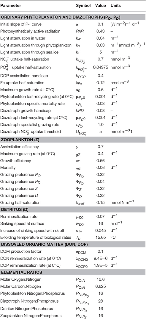
Table A1. Marine Ecosystem-Biogeochemistry Parameters.