Employing Predictive Spatial Models to Inform Conservation Planning for Seabirds in the Labrador Sea

Introduction

Offshore resource development has led to an increased need for understanding marine living resource abundance and distribution, and the effects of these activities on biota (Kark et al., 2015). These effects range from point sources and direct mortality (i.e., ship strikes, bottom draggers) to more generalized effects such as eutrophication, pollution, and ocean acidification (Jones, 1992; Laist et al., 2001; Shahidul Islam and Tanaka, 2004; Orr et al., 2005; Rabalais et al., 2009). However, obtaining the needed biological information is logistically challenging, especially in remote regions such as the Arctic (Arctic Council, 2009). Among marine organisms, seabirds are particularly vulnerable to a number of effects from marine industries, including being especially vulnerable to the effects of oil at sea (Wiese and Robertson, 2004; Votier et al., 2005) and other threats such as mortality in fisheries as bycatch (Žydelis et al., 2013; Hedd et al., 2016). Specific to oil pollution, determining the effect of a hydrocarbon release in remote marine environments is difficult when seabird densities in a particular area and season are not known (Wilhelm et al., 2007; Haney et al., 2014).

One such remote region is the Labrador Sea. The Labrador Sea contains significant oil and gas reserves and has been a focus of resource exploration for decades (AMAP, 2010). However, the demand for better baseline biological data to support regional scale environmental assessments (C-NLOPB, 2008) is more recent. The Labrador Sea is important to marine birds year-round supporting breeding seabird colonies during summer and providing important staging, migration, and wintering habitat for seabirds from colonies in both the northern and southern hemisphere (Brown, 1986; Huettmann and Diamond, 2000; Bakken and Mehlum, 2005). Recent tracking information shows movements of North Atlantic breeding seabirds to staging and wintering areas in eastern Canadian and Greenlandic waters that include the Labrador Sea, highlighting the international importance of these waters (Frederiksen et al., 2012, 2016; Mosbech et al., 2012; Fort et al., 2013; Jessopp et al., 2013; Linnebjerg et al., 2013; McFarlane Tranquilla et al., 2013). However, explicit local-scale spatial information on seabird distribution in the Labrador Sea has been limited by patchy marine survey coverage (Fifield et al., 2009), mostly due to logistical difficulties. Understanding the spatial and temporal extent of overlap of seabird populations with offshore resource activities will be critical to the environmental assessment process (Camphuysen et al., 2004; Fifield et al., 2009), and to understanding potential risks to seabirds.

Previous assessments of seabird distributions at sea were limited to the time and place where survey data were actually collected. Recent statistical advances in density surface modeling (DSM) provide an emerging framework that is capable of overcoming many of the constraints of earlier approaches while accounting for imperfect detection (Miller et al., 2013). Now, at-sea survey data are used directly to examine relationships between environmental covariates (generally collected by remote sensing) and seabird densities. Once these relationships are understood, predictions of seabird densities in areas of comparable environmental conditions are possible—even when there is no survey coverage in the immediate area (Miller et al., 2013).

The purpose of this paper is to explore the utility of DSM to meet the demand for better baseline biological data to inform conservation and management decision-making in the Labrador Sea. Specifically, we (1) develop seasonal DSMs for all seabird species combined in the Labrador Sea, (2) present measures of uncertainty in model predictions, (3) discuss how DSMs can aid in conservation and management decision making in the region, and (4) explore some of the challenges and potential pitfalls associated with using these complex modeling procedures.

Materials and Methods

Study Area

The study area (464,104 km²) is aligned with the Labrador Shelf Strategic Environmental Assessment (SEA) Area (C-NLOPB, 2008), defined using North Atlantic Fisheries Organization (NAFO) regions (2G, 2H, 2J) within the Canadian Exclusive Economic Zone (Figure 1).

FIGURE 1

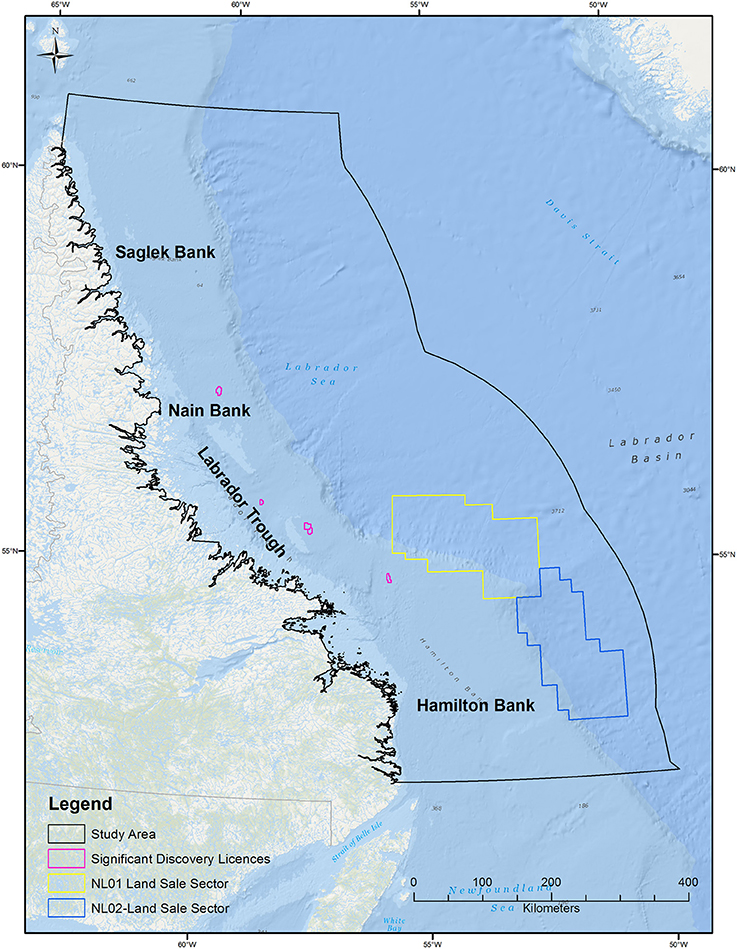
Figure 1. Labrador Sea study area, which encompasses the area of the Labrador Sea delineated by NAFO regions 2G, 2H, 2J, out to the Canadian EEZ (Exclusive Economic Zone). Significant discovery licenses and active C-NLOPB land issuance sectors in the Labrador Sea are also indicated.

Ship-Based Surveys

Surveys were conducted within the purview of Canadian Wildlife Service's Eastern Canada Seabirds At Sea (ECSAS) program, which follows a standardized protocol that incorporates Distance Sampling methods (Buckland et al., 2001; Fifield et al., 2009; Gjerdrum et al., 2012). Briefly, surveys consisted of a series of sequential observation periods (nominally 5-min duration) along a continuous line-transect, providing segments of mean length 1.64 km (SD: 0.61 km) as the sample unit for the DSM (see below). GPS coordinates were recorded at the beginning and end of each segment. Environmental variables that might be expected to affect bird detection such as wind speed and wave height were collected and updated at the beginning of each segment (Gjerdrum et al., 2012). We recorded observations of birds on the water continuously along each segment, and used a snapshot approach for flying birds (Tasker et al., 1984; Gjerdrum et al., 2012). Distance categories (0–50, 5–100, 100–200, 200–300 m; Gjerdrum et al., 2012) for each observation were assigned by estimating the perpendicular distance to each individual bird (or the centroid of each group of birds) with the help of a pre-marked custom ruler constructed for each observer-vessel combination (Gjerdrum et al., 2012). Data were entered directly into the ECSAS Microsoft Access database using voice recognition software or recorded on datasheets and entered into the database (Fifield et al., 2009).

Data Analysis

Data Extraction and Filtering

Survey data consistent with the methods described in Section Ship-Based Surveys were extracted from ECSAS database version 3.38. Only data collected from moving vessels whose speed exceeded 4 knots were included (Gjerdrum et al., 2012). Certain seabird species are attracted to fishing vessels, which can artificially inflate densities of these birds around such vessels. Therefore, observations of these taxa (i.e., gulls, Northern fulmar, shearwaters, and black-legged kittiwake) collected during Fisheries and Oceans Canada (DFO) scientific trawl surveys were removed prior to analysis (10 of 35 trips, see Supplementary Tables 1, 2).

Environmental covariates used in modeling

We modeled the density (or equivalently, abundance) of seabirds in the Labrador Sea relative to environmental variables (Table 1). These were chosen because each has been demonstrated to correlate with the distribution or abundance of seabirds at sea, or could be expected to correlate (Louzao et al., 2006, 2011; Wakefield et al., 2009; Oppel et al., 2012). To extract (or interpolate) values for all of the dynamic and most of the static variables associated with the starting position of each segment, we used Marine Geospatial Ecology Tools (MGET; Roberts et al., 2010) within ArcGIS (Table 1). Values of sea surface temperature (SST; JPL MUR MEaSUREs Project, 2010), and anomalies in both sea surface height (SSH), and eddy kinetic energy (EKE; AVISO, 2016) were extracted directly using MGET Data Products tools. To estimate spatial gradients in SST (SSTG), monthly rasters of SST climatology were first created, and gradients subsequently estimated as a proportional change (PC) within a surrounding 3 × 3 cell moving window following Louzao et al. (2006): PC = [(SST maximum value − SST minimum value) × 100]/(SST maximum value). SST minimum and maximum rasters were created from monthly climatologies using the Focal Statistics tool, with subsequent algebra executed using the Raster Calculator. Static environmental variables including bathymetry and its derivatives were determined from ETOPO2 grids (National Geophysical Data Center, 2006) which is based on satellite altimetry and shipborne ground-truthing measurements. The spatial gradient in bathymetry (BathyG) was estimated as indicated above for the gradient in SST, and distance to the continental shelf break (Dist1000, defined as the 1,000 m contour) was calculated using the Near tool within ArcGIS Analysis toolset. To avoid collinearity among these covariates, we assessed both seasonal and overall variance inflation factors to ensure that they were all below 3 (Zuur et al., 2010), and to ensure that the absolute value of all Pearson correlation coefficients between pairs of explanatory variables were <0.52 which is below the 0.7 threshold where collinearity has been shown to severely effect model predictions (Dormann et al., 2013).

TABLE 1

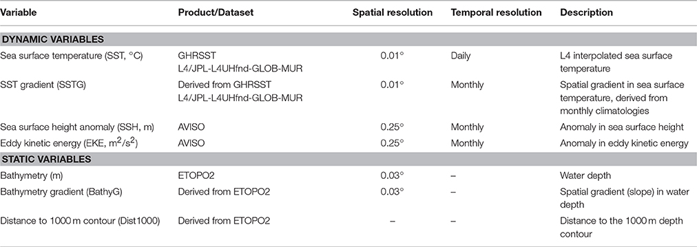
Table 1. List of environmental variables used to model the density of seabirds within the Labrador Sea.

Environmental data used to predict seabird abundance or density

Each cell within a 2 × 2 km prediction grid covering the study area was populated with the static variables listed in Table 1, along with seasonally-averaged values for the dynamic covariates recorded over the 10-year period between 2005 and 2014. Seasons were defined as Summer (June–August), Fall (September–October), Winter (November–March), and Spring (April–May). To generate these dynamic covariate layers, we first used MGET Data Products tools to create monthly rasters for the period January 2005 to December 2014, and then the ArcGIS Raster calculator tool (Spatial Analyst toolset) to create seasonal averages. Seasonal spatial gradients in SST were calculated as indicated above for the modeling step, but using the seasonally averaged SST rasters as input. Values for the prediction grid were obtained using an MGET Spatial and Temporal Analysis tool (“Project Raster to Template”), which projected each environmental raster to the coordinate system, cell size and extent of the prediction grid (Lambert Azimuthal Equal Area projection).

Modeling Approach

We conducted an analysis for all seabird species combined (Fifield et al., 2016) producing a seasonal spatial predictive model in R 3.2.3 (R Core Team, 2016) following a two-stage DSM approach (Hedley and Buckland, 2004; Miller et al., 2013) using the Distance v. 0.9.4 (Miller, 2015), dsm v. 2.2.13 (Miller et al., 2015), and mgcv v. 1.8–17 R packages.

Stage 1

In Distance Sampling, the process of fitting a detection function accounts for the fact that some birds are unavoidably missed during surveys (Buckland et al., 2001). A detection function was fitted by modeling detectability as a function of distance from the observer and other covariates including observer identity, species (or guild), flock size, wind speed, wave height, season, and bird behavior (i.e., flying or on the water). The best detection function model was selected using Akaike Information Criteria (AIC), and model fit was assessed using plots of detection function fit to the distance histogram, and through χ² goodness-of-fit tests. The best detection function was then used to correct the estimated density of seabirds present in each survey segment (Hedley and Buckland, 2004).

Stage 2

We constructed seasonal Generalized Additive Models (GAMs, Wood, 2006) of density as a function of environmental covariates in surveyed areas. GAMs were fitted to the density data using quassiPoisson, negative binomial and Tweedie response distributions.

For each distribution, an initial full model was fitted containing seasonal thin-plate regression spline smooths (Wood, 2006). Dynamic variables (EKE, SSH, SST, SSTG; Table 1) were fitted with a single smooth to allow the natural variation within and across seasons to inform the fit. We allowed for a seasonal time component for static variables (Bathy, BathyG, Dist1000), which have no natural seasonal variation, in GAM fitting (through use of the mgcv “by = Season” option). A parametric (i.e., non-smooth) term for each season was also initially included in all models. QQ-plots of initial full models using each of the three response distributions indicated the negative binomial distribution provided a superior fit and the other distributions were not considered further.

Model refinement progressed by iterative backwards selection of the full negative binomial model refining all smooth terms first, followed by parametric terms. At each iteration, the remaining smooth term with the lowest estimated degrees of freedom (EDF; or sum of the four individual component EDFs for seasonal smooths) less than 1.5 was considered for removal, or replacement by a linear parametric term. The term was replaced by a parametric one if the slope of the coefficient was significantly different from 0 (i.e., if its p ≤ 0.01) or removed otherwise. Seasonal smooth terms were replaced by parametric terms with an interaction with season to allow the slope of the linear relationship to vary seasonally. Refinement of parametric terms consisted of removing those whose p ≥ 0.01, and interactions were removed before main effects.

Autocorrelation was assessed via a plot of correlations in the residuals at lags of 1–20 consecutive segments, by inspection of variograms of the residuals at scales of 2, 5, 10, and 100 km, and visual inspection of spatial plots of residuals (bubble plots from R package sp v. 1.2-4).

We used the final fitted model to predict and map seasonal density in a 2 × 2 km grid-cell matrix over the entire study area using the same environmental covariates. The spatial resolution of this grid was chosen to match the segment length. Mapping of model uncertainty in individual grid cells, as measured by the coefficient of variation (CV), was computed at a lesser resolution of 6 × 6 km due to computer memory constraints.

Seasonal Densities and Population Estimates

Two seasonal density (birds·km⁻²) and population estimates were produced: one for the entire study area and a second excluding areas of environmental extrapolation beyond the range of sampled covariates used to build the models. Extrapolations outside these ranges are largely speculative and such areas have been indicated in Figure 2 with crosshatches to appropriately caution the reader (Mannocci et al., 2016). These areas varied seasonally. Further, large portions of the study area may be covered by ice in winter, spring, and summer and therefore be unavailable for seabirds. We removed these areas from density and population estimates by obtaining ArcGIS shapefiles containing weekly climatologies of median ice concentration for the East Coast and Northern Canadian Waters for the period 1981–2010, as compiled by the Canadian Ice Service (http://ec.gc.ca/glaces-ice/). To be conservative, we were interested in the maximum seasonal median ice extent where ice concentrations exceeded 9−9+ (i.e., waters that were >90% ice covered), and so these concentrations were selected and the ArcGIS Merge tool (Data Management Tools) was used to create a single polygon for each season.

FIGURE 2

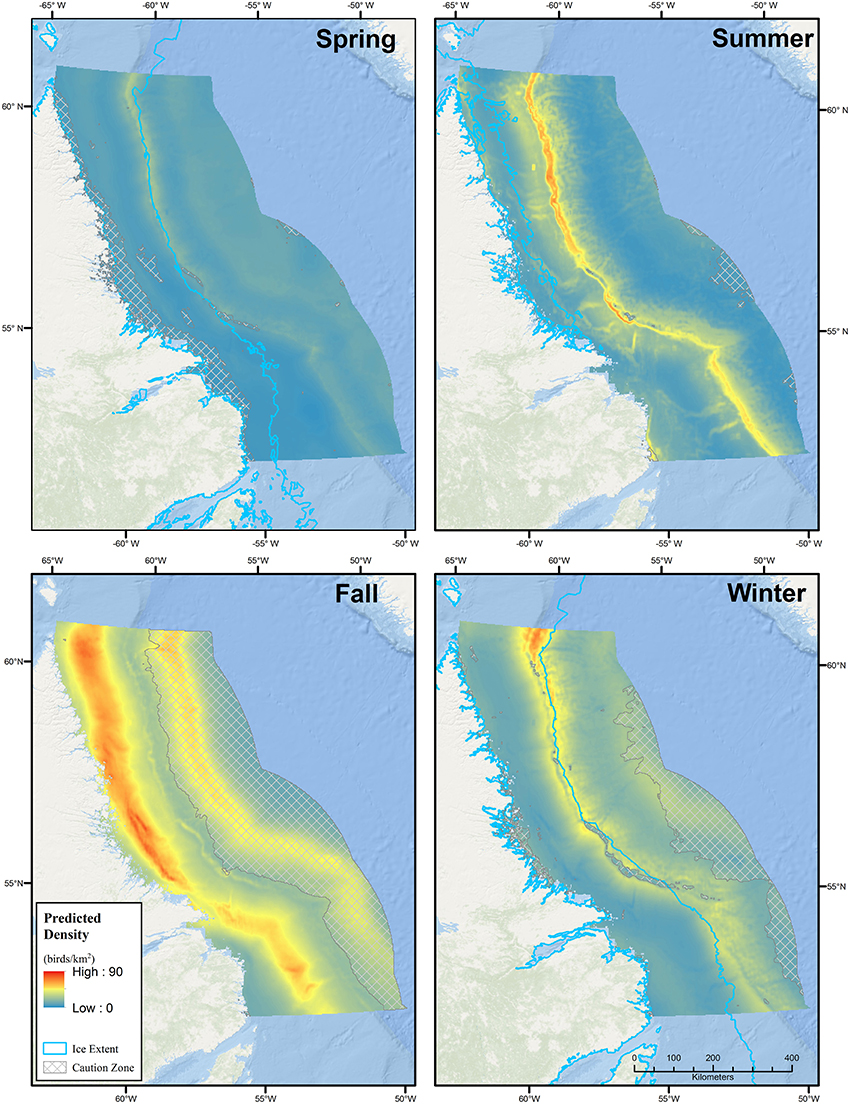
Figure 2. Seasonal predicted densities of all seabirds based on Generalized Additive Models (GAMs). Areas of extrapolation beyond the range of model covariates are indicated with crosshatching. Seasons are defined as Summer (June–August), Fall (September–October), Winter (November–March), and Spring (April–May).

Sensitivity Analysis

We conducted a sensitivity analysis by individually removing each covariate from the final fitted DSM. For each reduced model, a new set of seasonal maps and population estimates were produced and compared with the results from the full model.

Results

From May 2006 to November 2014, observers surveyed 13,783 linear km, or 4,135 km² (8,392 segments) for seabirds within the Labrador Sea study area, with the most intensive effort occurring between 2012 and 2014. Surveys were conducted during all seasons; however, as survey platforms were largely ships of opportunity, effort was distributed unevenly across the study area by season (Figure 3). The most complete spatial coverage was achieved in summer, when surveys were conducted from Saglek Bank in the north to Hamilton Bank in the south, both on and off the Labrador Shelf, while the poorest spatial coverage occurred in winter when most surveys were concentrated in the south in the vicinity of Hamilton Bank (Figure 3). Effort was most intense in fall, with shelf waters south of and including the Nain Bank being well-surveyed. Seasonal differences in the spatial distribution and intensity of survey effort have implications for the precision of seabird density estimates, as demonstrated below.

FIGURE 3

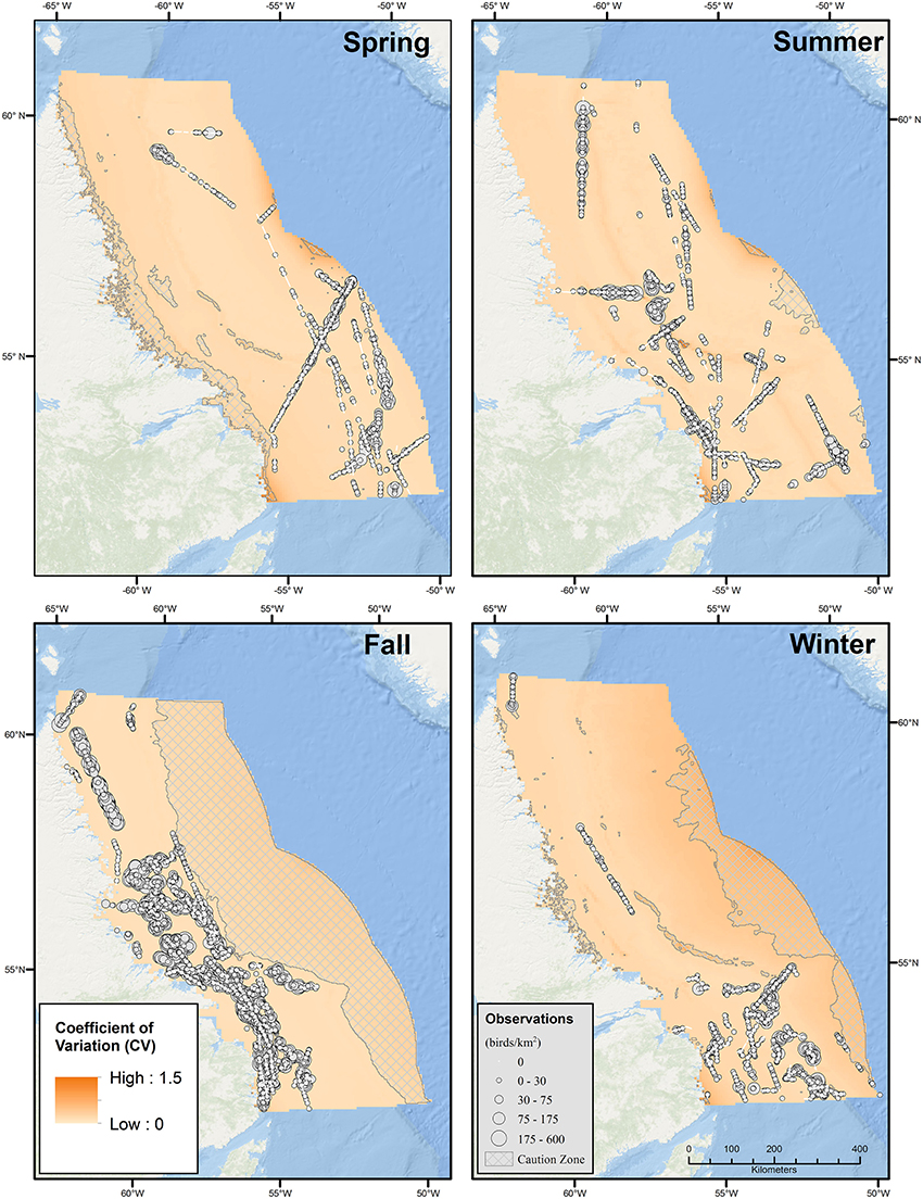
Figure 3. Seasonal bird observations and coefficient of variation (CV) for predicted densities of all seabirds based on Generalized Additive Models (GAMs). Seasons were defined as Summer (June-August), Fall (September-October), Winter (November-March), and Spring (April-May).

In total, ship surveys detected 33,469 seabirds (12,379 flocks) in 4,638 of 8,392 (55%) segments, with dovekie (Alle alle), northern fulmar (Fulmarus glacialis), black-legged kittiwake (Rissa tridactyla), and murres (Uria spp.) being the taxa most frequently observed (see Supplementary Tables 3, 4 for a complete list of observed species).

Modeling

The best detection function model contained a hazard-rate key function and covariates for taxon, wind, wave height, bird behavior (flying or on water), season, and flock size. Average detection probability was 38% (CV = 0.26), indicating that failure to adopt a distance sampling methodology would have underestimated seabird densities in each surveyed segment by an average of 2.6 times. For the density surface model, a negative binomial distribution with dispersion parameter k = 0.248 provided the best fit to the data explaining 17.6% of the deviance. Retained smooth terms included Bathymetry, BathyG, Dist1000, EKE, SST, and SSH, along with the parametric Season term (see Supplementary Figure 1 model output and plots of regression splines).

Residual autocorrelation at lags of 1–20 segments was relatively low (all r < 0.2), and variograms and spatial plots of residuals showed no obvious patterns.

Predicted Densities and Population Estimates

The Labrador Shelf and adjacent portions of the Labrador Sea are clearly important regions for seabirds, particularly during fall and winter, when densities were 33.9 (CV = 0.26) birds·km⁻² and 21.6 (CV = 0.37) birds·km⁻², respectively (Table 2, Figure 2). During fall and winter, the estimated number of seabirds in the region (to the nearest 100,000) were 15.4 million (95% CI: 9.3–25.5 million) and 5.3 million (95% CI: 2.6–10.9 million), respectively. During fall, relatively high densities were predicted throughout the Labrador Shelf, from the Saglek and Nain Banks south to the Labrador Trough. Predicted densities in a substantial portion of the Saglek Bank and Labrador Trough exceeded 50–75 birds·km⁻² in fall. Areas with high predicted densities in fall overlapped with several significant hydrocarbon discoveries on the Labrador Shelf (Figures 1, 2). Somewhat lower bird densities were predicted in offshore regions in fall; however, the lack of survey coverage in these areas lowers confidence in the predictions. During winter, the model predicted high densities (>25 birds·km⁻²) all along the continental shelf break. In summer, mean density was 15.3 (0.25) birds·km⁻² and particularly high densities were also predicted along the shelf break, with a noticeable peak in the very north. The regional seabird population estimate in summer was 6.4 million (95% CI: 3.9–10.5 million). Predicted densities and numbers of birds were lower overall during spring, and averaged 9.0 (CV = 0.26) birds·km⁻² and 2.7 million (95% CI: 1.6–4.4 million) birds (Table 2). Mean (range) CVs (6 × 6 km cells) were 0.19 (0.13–1.14) in spring, 0.20 (0.14–1.50) in summer, 0.19 (0.11–0.52) in fall, and 0.36 (0.16–0.85) in winter (Figure 3).

TABLE 2

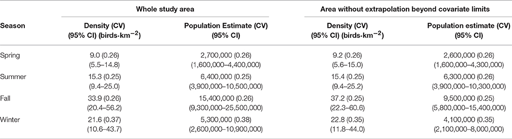
Table 2. Seasonal densities and population estimates (to the nearest 100,000) excluding ice-covered areas for the entire study area and for the area without extrapolation beyond range of model covariates (see Figure 2).

Sensitivity Analysis

Density and abundance estimates were insensitive to removal of individual model terms; confidence intervals for these quantities all overlapped extensively for all models (Supplementary Figure 2). The spatial density pattern was also similar across all models, with the greatest differences evident in fall for models without Dist1000 and Season (Supplementary Figure 3). Likewise, spatial uncertainty patterns were similar across all models except during fall for the model without Dist1000 where uncertainty off the continental shelf (where there was no sampling) was greater than in other models (Supplementary Figure 4).

Modeling and Interpretation Challenges

Areas of extrapolation where the values of environmental predictors were beyond the range of those covariates in the model occurred to varying degrees across seasons (crosshatched in Figure 2). In the majority of cases, this was caused by a lack of vessel-survey coverage in those water depths during those seasons. Predicted densities in these areas must be interpreted with extreme caution. This is of particular interest to the current application since much of the continental slope and deep offshore area, particularly in the southeast, is in the early stages of hydrocarbon exploration. The lack of survey coverage in these regions highlights a priority data gap.

DSM fitting, spatial prediction and variance computation was both CPU and memory intensive. For example, this process typically required 1–2 h for a single run to complete on a Lenovo laptop with an Intel Core i5-3320M processor running at 2.6 GHz with 8 GB ram utilizing all four processors in parallel. During the per-cell prediction and variance calculation steps the R process memory requirements typically grew to more than 4 GB at a 6 × 6 km scale. Attempts to compute the variance at a 2 × 2 km scale failed when R attempted to allocate more than 96 GB of memory.

Discussion

The purpose of this study was to explore the utility of DSM to inform conservation and management needs of seabirds in the Labrador Sea. This is of particular importance given domestic and international commitments to protect 10% of coastal and ocean areas by 2020 (CBD, 2010) and the regional increase in industrial activity. Using at-sea seabird survey data collected onboard ships of opportunity, seasonal models of seabird distribution and abundance were built throughout the region. These will contribute to the baseline information needed for quantitative environmental assessments which precede development of the offshore hydrocarbon industry. While data collection within oil and gas significant discovery license areas themselves was sometimes sparse, by utilizing this relatively recent statistical approach (Miller et al., 2013), models built from data collected in nearby regions enabled plausible predictions of seabird densities throughout much of the area of interest. We expect these outputs will inform future conservation and management decision making in the Labrador Sea and contribute to conservation targets. In addition to marine protected area planning and offshore oil and gas exploration and production, understanding risks from shipping (and associated risk of hydrocarbon releases) and mortality from fishing activities can all be improved by these models.

Our results indicate millions of seabirds use the Labrador Sea at all times of year, with especially high concentrations over the shelf regions in the fall. This is consistent with known migration patterns of seabirds in the North Atlantic. Many of the 3 million breeding thick-billed murres from Canadian colonies (Gaston et al., 2012) migrate along the Labrador Shelf to winter in low arctic regions (McFarlane Tranquilla et al., 2013) and large numbers (~850,000) of thick-billed murres from colonies spanning the eastern and western North Atlantic winter in the Labrador Sea (Frederiksen et al., 2016). Similarly, black-legged kittiwakes from colonies spanning the North Atlantic use the Labrador Sea in winter, especially waters off the shelf edge (Frederiksen et al., 2012). Dovekie are the most numerous seabird in Northwest Atlantic waters, and millions of breeding birds from West Greenland colonies migrate south through the Labrador Sea to wintering grounds off Newfoundland (Fort et al., 2013).

In terms of conservation planning, our models have the ability to inform and refine the boundaries of Ecologically and Biologically Significant Areas (EBSAs) recently defined for the Newfoundland and Labrador Shelves Bioregion (DFO, 2013; Figure 4). The most recent EBSA delineation process for the Labrador Shelf included seabird data collected from pelagic surveys (DFO, 2013), but this data was very coarse and lacked spatial and temporal coverage across much of the Labrador Sea (Fifield et al., 2009). Our analysis shows the importance of the fall migration period for seabirds, especially along the northern parts of the shelf. Portions of this region are covered by the Northern Labrador and the Hopedale Saddle EBSAs (DFO, 2013) but important areas of ocean for seabirds between these two EBSAs are not included. A portion of the important summer concentration of seabirds along the shelf break at the northern part of the study area is included in the Outer Shelf Saglek Bank EBSA, and concentrations of wintering seabirds are within the Labrador Slope EBSA, which covers a large stretch of ocean along the shelf edge in the middle of the study area (DFO, 2013). As Canada progresses with Marine Protected Area planning exercises to meet Convention on Biological Diversity (CBD) targets (Secretariat of the Convention on Biological Diversity the Scientific Technical Advisory Panel—GEF, 2012), our results can be used to further refine EBSA and subsequent Marine Protected Area boundaries. Since these models have a temporal component, boundaries can be created that are dynamic, for example they may change with seasons, or can be changed if future data indicates a significant shift in marine bird concentrations.

FIGURE 4

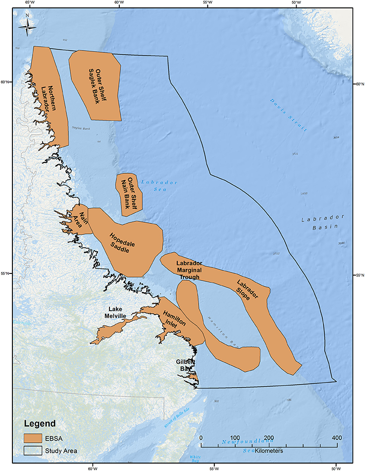
Figure 4. Ecologically and Biologically Significant Areas (EBSA) within the study area (DFO, 2013).

Our analysis considered all seabirds in the Labrador Sea combined. However, different seabird guilds have different relative risks to specific types of threats in the marine environment (e.g., Wiese and Robertson, 2004; Good et al., 2009; O'Hara et al., 2009; Hedd et al., 2016). Predictive modeling at the guild or species level is important to inform risk and damage assessments for seabirds (Le Rest et al., 2016; Fox et al., 2017). Future studies should address this gap by constructing DSMs on a per guild (or species) basis to better inform management and conservation for marine birds in the Labrador Sea.

A number of static (Bathymetry, BathyG, Dist1000) and dynamic (EKE, SST, SSTG, SSH) oceanographic features we selected were retained in the model as predictors of seabird densities and explained 18% of deviation in the data. Previously, several of these features had been identified as important predictors of at-sea densities for other top predators (Mannocci et al., 2016). This clearly, and not unexpectedly, indicates that the density of seabirds are not uniform in time or space on the Labrador Sea, and smaller scale estimation will provide better estimates of seabird density at scales relevant to marine resource planners and to development of conservation policy. During fall, high predicted densities occurred in relatively shallow waters throughout the continental shelf. In both the summer and winter, however, highest predicted densities occurred along the shelf break and slope, habitat features which have been shown to be important for seabirds in other regions (Catard et al., 2000; Croxall and Wood, 2002). Specific to oil and gas exploration, significant discovery licenses which are on the continental shelf midway along the Labrador coast, overlap with high predicted densities of seabirds, notably in the fall. Predicted seabird densities in areas of interest to the oil and gas sector in the southeastern part of the Labrador Sea identified large areas where birds concentrated during fall and winter, and to a lesser extent during spring and summer. However, in the fall, surveys were restricted to the continental shelf, precluding us from obtaining high confidence in the density estimates in these areas of interest to the oil and gas industry. The best approach for addressing these remaining data gaps would be a designed survey approach that targets high priority areas, as opposed to opportunistic surveys.

Caution and an understanding of the uncertainty associated with model predictions is vital when interpreting DSM-predicted density output. To facilitate appropriate interpretation we produced companion maps of associated uncertainty (in our case, using the CV or coefficient of variation; see also Winiarski et al., 2014; Mannocci et al., 2016), to be viewed alongside fine-scale maps of predicted seabird densities. These maps are to be interpreted in tandem, to highlight seasons and areas where model predictions are associated with higher degrees of uncertainty. In modeling seabirds in the Labrador Sea, the overall range of per-cell CVs was modest with similar precision achieved during spring, summer and fall, and lesser precision in winter with relative differences being driven by seasonal sample sizes. Within each season, the CV tended to increase toward the edges of the study area where some covariates approached the limit of their ranges and so corresponding predictions were less precise.

Large areas of ocean featured environmental extrapolation beyond the range of model covariates, and predictions in these areas must be interpreted with caution (e.g., in deep off-shelf waters during fall and winter). The tendency for GAMs to produce extreme predictions at or beyond the limits of covariate values is well-known (Mannocci et al., 2016). For example, in a previous modeling exercise (Fifield et al., 2016) we included the X and Y coordinates (projected longitude and latitude, respectively) as covariates in our GAMs. However, much of the study area was outside the X and Y range of sampling in one or more seasons leading to extreme predicted densities and low precision. It is thus apparent that the choice of model covariates strongly affects predicted densities and their precision. To draw the reader's attention to this fact in the current analysis, areas of extrapolation have been crosshatched in the prediction surfaces (cf. Mannocci et al., 2016). It can be important to dig deeper and understand which environmental predictor(s) cause the extrapolation, and to what extent they affect predicted densities in such areas. For example, during fall there is a considerable area of moderately high predicted densities (up to 50 birds·km⁻²) in deep off-shelf waters in the northeast where extrapolation is due to a lack of seabird survey effort in deep waters. However, examining the fall regression spline plot for Bathymetry from the GAM output (Supplementary Figure 1) indicates that water depth had no effect on predicted density during this season due to a nearly flat relationship centered at 0. However, Bathymetry was retained in the model due to a significant interaction effect in other seasons. This highlights the tradeoffs inherent between pooling all data in a single model with seasonal interactions vs. modeling each season separately where data may be sparse in some seasons. Instead, these high predicted densities are a result of the Dist1000 model term. Thus an intimate knowledge of modeled relationships may be required to interpret crosshatched plots of environmental extrapolation (cf. Mannocci et al., 2016) and this may guide the degree of caution required in interpreting predictions in such areas. Nonetheless, a qualitative assessment of prediction plausibility should be undertaken in the context of other sources of distribution and abundance information (see below and Mannocci et al., 2016).

Sensitivity analysis indicated that the model was relatively insensitive to single-term deletions with density and population estimate confidence intervals overlapping for all models. Likewise spatial patterns of density and uncertainty (CV) were similar across all models except for in deep off-shelf waters during fall for 2 models; an area where bathymetric extrapolation occurred due to lack of fall deep-water survey coverage. Improving survey effort in this area would likely help to limit model sensitivity.

Residual spatial autocorrelation can bias analyses by inflating Type I error rates, and a variety of statistical methods have been proposed to account for this fact (Dormann et al., 2007; Bivand et al., 2015). Similar to Winiarski et al. (2013), un-modeled residual autocorrelation was relatively low in this study and we feel confident that it did not unduly bias our results. Nonetheless, future work should investigate methods to accommodate autocorrelation.

When deciding whether to use DSM, considerations include the non-trivial commitments of time and computer resources required to execute these complicated techniques. The time required to fit and visualize prediction and uncertainty outputs should not be underestimated, especially when comparing many candidate models across multiple species groups (Fifield et al., 2016). Computing variance for DSM predictions is memory intensive, particularly for large study areas with small grid-cell sizes and may stretch computing resources beyond available limits. Approaches to streamline the process could involve using multiple computers running in parallel, using a centralized high performance computing server environment, or processing the study area in a series of sub-areas and combining the results (although this further complicates the analysis). The statistical approaches involved in DSM are an active area of research (Hedley and Buckland, 2004; Miller et al., 2013), but all are based on advanced techniques and extensive experience and training are required. These are not readily accessible to all and likely help to explain the gap between having data and using data to best inform critical environmental assessment processes, both in the Labrador sea, and in other marine areas of concern where survey coverage may be limited. These caveats notwithstanding, we believe DSMs are a valuable approach to inform seabird conservation over large areas of ocean where survey coverage is incomplete, and would recommend that management agencies develop capacity and expertise in this or similar predictive modeling approaches.

Author Contributions

DF: developed project design, secured funding, contributed to data collection, lead the data analysis, and co-wrote the manuscript. AH: contributed both to data analysis and to the writing of the manuscript. SA: developed project design, contributed to data collection, analysis and editing of the manuscript. GR: developed project design, secured funding, managed project through completion and contributed to the writing of the manuscript. CG: coordinated data collection and observer training, and managed the ECSAS database. LM: contributed to data collection, project management (field logistics), editing the manuscript.

Funding

Funding for this project was received from the Environmental Studies Research Funds (ESRF; project 2010-08S) and Environment and Climate Change Canada.

Conflict of Interest Statement

The funding base for the Environmental Studies Research Funds (ESRF) is provided through levies on frontier lands paid by interested holders such as oil and gas companies. However, the ESRF is directed by a joint government/industry/public Management Board and administered by a secretariat in the Office of Energy Research and Development, Natural Resources Canada, and remains at arm's length from this project and its findings.

Acknowledgments

We thank the Environmental Studies Research Funds (ESRF), Dave Taylor (ESRF Secretariat) for funding, guidance and support. Access to survey vessels was kindly provided in part by DFO chief scientists and CCGS captains, Joey Angnotok, and Putjotik Fisheries Ltd. We thank the many dedicated observers who spent long hours collecting data in often less than ideal weather conditions, and the captains and crews for their hospitality. We thank the following for many insightful conversations regarding study design, data collection, and analysis and mapping approaches: François Bolduc, Steven Duffy, Jack Lawson, Ken Morgan, Pat O'Hara, Rob Ronconi, Christian Roy, Pierre Ryan, Sabina Wilhelm and Sarah Wong. We thank two reviewers for comments that improved the quality of the paper.

Supplementary Material

The Supplementary Material for this article can be found online at: https://www.frontiersin.org/article/10.3389/fmars.2017.00149/full#supplementary-material

References

AMAP (2010). Assessment 2007: Oil and Gas Activities in the Arctic – Effects and Potential Effects. Vol. 1. Oslo: Arctic Monitoring and Assessment Programme (AMAP), 423.

AVISO (2016). Ssalto/Duacs Altimeter Products. Copernicus Marine and Environment Monitoring Service (CMEMS). Available online at: http://www.marine.copernicus.eu (Accessed November 05, 2015).

Arctic Council (2009). Arctic Marine Shipping Assessment 2009 Report. Protection of the Marine Environment (PAME) and the Arctic Council.

Bakken, V., and Mehlum, F. (2005). Wintering areas and recovery rates of Brunnich's guillemots (Uria lomvia) ringed in the Svalbard archipelago. Arctic 58, 268–275. doi: 10.14430/arctic428

CrossRef Full Text | Google Scholar

Bivand, R., Gomez-Rubio, V., and Rue, H. (2015). Spatial data analysis with R-INLA with some extensions. J. Stat. Softw. 63, 1–31. doi: 10.18637/jss.v063.i20

CrossRef Full Text | Google Scholar

Brown, R. G. B. (1986). Revised Atlas of Eastern Canadian Seabirds. Ottawa, ON: Canadian Wildlife Service.

Buckland, S. T., Anderson, D. R., Burnham, K. P., Laake, J. L., Borchers, D. L., and Thomas, L. (2001). Introduction to Distance Sampling: Estimating Abundance of Wildlife Populations. Oxford: Oxford University Press.

Camphuysen, K., Fox, A. D., Leopold, M. F., and Petersen, I. K. (2004). Towards Standardised Seabirds at Sea Census Techniques in Connection with Environmental Impact Assessments for Offshore Wind Farms in the U.K. COWRIE-BAM 02-2002. Royal Netherlands Institute for Sea Research, 39.

Catard, A., Weimerskirch, H., and Cherel, Y. (2000). Exploitation of distant Antarctic waters and close shelf-break waters by white-chinned petrels rearing chicks. Mar. Ecol. Prog. Ser. 194, 249–261. doi: 10.3354/meps194249

CrossRef Full Text | Google Scholar

CBD (2010). Aichi Biodiversity Targets. Available online at: https://www.cbd.int/sp/targets/ (Accessed January 25, 2017).

PubMed Abstract

C-NLOPB (2008). Strategic Environmental Assessment Labrador Shelf Area. Canadian Newfoundland and Labrador Offshore Petroleum Board (C-NLOPB) Final Report. 86. Available online at: www.C-NLOPB.nl.ca/news/nr20080828.eng.shtml

Croxall, J. P., and Wood, A. G (2002). The importance of the Patagonian Shelf for top predator species breeding at South Georgia. Aquat. Conserv. Mar. Freshw. Ecosyst. 12, 101–118. doi: 10.1002/aqc.480

CrossRef Full Text | Google Scholar

DFO (2013). Identification of Additional Ecologically and Biologically Significant Areas (EBSAS) within the Newfoundland and Labrador Shelves Bioregion. DFO Canadian Science Advisory Secretariat Science Advisory Report. Report 2013/048.

Dormann, C. F., McPherson, J. M., Araújo, M. B., Bivand, R., Bolliger, J., Carl, G., et al. (2007). Methods to account for spatial autocorrelation in the analysis of species distributional data: a review. Ecography 30, 609–628. doi: 10.1111/j.2007.0906-7590.05171.x

CrossRef Full Text

Dormann, C. F., Elith, J., Bacher, S., Buchmann, C., Carl, G., Carré, G., et al. (2013). Collinearity: a review of methods to deal with it and a simulation study evaluating their performance. Ecography 36, 27–46. doi: 10.1111/j.1600-0587.2012.07348.x

CrossRef Full Text | Google Scholar

Fifield, D. A., Hedd, A., Robertson, G. J., Avery-Gomm, S., Gjerdrum, C., McFarlane Tranquilla, L. A., et al. (2016). Baseline Surveys for Seabirds in the Labrador Sea (201-08S). Environmental Studies Research Funds Report No. 205. St. John's, NL. 42.

Fifield, D. A., Lewis, K. P., Gjerdrum, C., Robertson, G. J., and Wells, R. (2009). Offshore Seabird Monitoring Program. Environment Studies Research Funds Report No. 183. St. John's, NL. 68.

Frederiksen, M., Moe, B., Daunt, F., Phillips, R. A., Barrett, R. T., Bogdanova, M. I., et al. (2012). Multicolony tracking reveals the winter distribution of a pelagic seabird on an ocean basin scale. Divers. Distrib. 18, 530–542. doi: 10.1111/j.1472-4642.2011.00864.x

CrossRef Full Text | Google Scholar

Frederiksen, M., Descamps, S., Erikstad, K. E., Gaston, A. J., Gilchrist, H. G., Grémillet, D., et al. (2016). Migration and wintering of a declining seabird, the thick-billed murre Uria lomvia, on an ocean basin scale: conservation implications. Biol. Conserv. 200, 26–35. doi: 10.1016/j.biocon.2016.05.011

CrossRef Full Text | Google Scholar

Fort, J., Moe, B., Strøm, H., Grémillet, D., Welcker, J., Schultner, J., et al. (2013). Multicolony tracking reveals potential threats to little auks wintering in the North Atlantic from marine pollution and shrinking sea ice cover. Divers. Distrib. 19, 1322–1332. doi: 10.1111/ddi.12105

CrossRef Full Text | Google Scholar

Fox, C. H., Huettmann, F. H., Harvey, G. K. A., Morgan, K. H., Robinson, J., Williams, R., et al. (2017). Predictions from machine learning ensembles: marine bird distribution and density on Canada's Pacific coast. Mar. Ecol. Prog. Ser. 566, 199–216. doi: 10.3354/meps12030

CrossRef Full Text | Google Scholar

Gaston, A. J., Mallory, M. L., and Gilchrist, H. G. (2012). Population status and trends of Canadian Arctic seabirds. Polar Biol. 35, 1221–1232. doi: 10.1007/s00300-012-1168-5

CrossRef Full Text | Google Scholar

Gjerdrum, C., Fifield, D. A., and Wilhelm, S. I. (2012). Eastern Canada Seabirds at Sea Standardized Protocol for Pelagic Seabird Surveys from Moving and Stationary Platforms. Canadian Wildlife Service Technical Report Series 515. Atlantic Region. 37.

Good, T. P., June, J. A., Etnier, M. A., and Broadhurst, G. (2009). Ghosts of the Salish Sea: threats to marine birds in Puget Sound and the Northwest Straits from derelict fishing gear. Mar. Ornithol. 37, 67–76.

Google Scholar

Haney, J. C., Geiger, H. J., and Short, J. W. (2014). Bird mortality from the Deepwater Horizon oil spill. I. Exposure probability in the offshore Gulf of Mexico. Mar. Ecol. Progr. Ser. 513, 225–237. doi: 10.3354/meps10991

CrossRef Full Text | Google Scholar

Hedd, A., Regular, P. M., Wilhelm, S. I., Rail, J.-F., Drolet, B., Fowler, M., et al. (2016). Characterization of seabird bycatch in eastern Canadian waters, 1998-2011, assessed from onboard fisheries observer data. Aquat. Conserv. Mar. Freshw. Ecosyst. 26, 530–548. doi: 10.1002/aqc.2551

CrossRef Full Text | Google Scholar

Hedley, S. L., and Buckland, S. T. (2004). Spatial models for line transect sampling. J. Agric. Biol. Environ. Stat. 9, 181–199. doi: 10.1198/1085711043578

CrossRef Full Text | Google Scholar

Huettmann, F., and Diamond, A. W. (2000). Seabird migration in the Canadian northwest Atlantic Ocean: moulting locations and movement patterns of immature birds. Can. J. Zool. 78, 624–647. doi: 10.1139/z99-239

CrossRef Full Text | Google Scholar

JPL MUR MEaSUREs Project (2010). GHRSST Level 4 MUR Global Foundation Sea Surface Temperature Analysis. Ver. 2. PODAAC (Accessed November 5, 2015). Available online at: https://podaac.jpl.nasa.gov/dataset/JPL-L4UHfnd-GLOB-MUR

Jessopp, M. J., Cronin, M., Doyle, T. K., Wilson, M., McQuatters-Gollop, A., Newton, S., et al. (2013). Transatlantic migration by post-breeding puffins: a strategy to exploit a temporarily abundant food resource? Mar. Biol. 160, 2755–2762. doi: 10.1007/s00227-013-2268-7

CrossRef Full Text | Google Scholar

Jones, J. B. (1992). Environmental impact of trawling on the seabed: a review. N. Z. J. Mar. Freshw. Res. 26, 59–67. doi: 10.1080/00288330.1992.9516500

CrossRef Full Text | Google Scholar

Kark, S., Brokovich, E., Mazor, T., and Levin, N. (2015). Emerging conservation challenges and prospects in an era of offshore hydrocarbon exploration and exploitation. Conserv. Biol. 29, 1573–1585. doi: 10.1111/cobi.12562

PubMed Abstract | CrossRef Full Text | Google Scholar

Laist, D. W., Knowlton, A. R., Mead, J. G., Collet, A. S., and Podesta, M. (2001). Collisions between ships and whales. Mar. Mamm. Sci. 17, 35–75. doi: 10.1111/j.1748-7692.2001.tb00980.x

CrossRef Full Text | Google Scholar

Le Rest, K., Certain, G., Debétencourt, B., and Bretagnolle, V. (2016). Spatio-temporal modelling of auk abundance after the Erika oil spill and implications for conservation. J. Appl. Ecol. 53, 1862–1870. doi: 10.1111/1365-2664.12686

CrossRef Full Text | Google Scholar

Linnebjerg, J. F., Fort, J., Guilford, T., Reuleaux, A., Mosbech, A., and Frederiksen, M. (2013). Sympatric breeding auks shift between dietary and spatial resource partitioning across the annual cycle. PLoS ONE 8:e72987. doi: 10.1371/journal.pone.0072987

PubMed Abstract | CrossRef Full Text | Google Scholar

Louzao, M., Hyrenbach, K. D., Arcos, J. M., Abelló, P., de Sola, L. G., and Oro, D. (2006). Oceanographic habitat of an endangered Mediterranean procellariiform: implications for marine protected areas. Ecol. Appl. 16, 1683–1695. doi: 10.1890/1051-0761(2006)016[1683:OHOAEM]2.0.CO;2

PubMed Abstract | CrossRef Full Text | Google Scholar

Louzao, M., Pinaud, D., Péron, C., Delord, K., Wiegand, T., and Weimerskirch, H. (2011). Conserving pelagic habitats: seascape modelling of an oceanic top predator. J. Appl. Ecol. 48, 121–132. doi: 10.1111/j.1365-2664.2010.01910.x

CrossRef Full Text | Google Scholar

Mannocci, L., Roberts, J. J., Miller, D. L., and Halpin, P. N. (2016). Extrapolating cetacean densities to quantitatively assess human impacts on populations in the high seas. Conserv. Biol. 31, 601–614. doi: 10.1111/cobi.12856

PubMed Abstract | CrossRef Full Text | Google Scholar

McFarlane Tranquilla, L., Montevecchi, W. A., Hedd, A., Fifield, D. A., Burke, C. M., Smith, P. A., et al. (2013). Multiple-colony winter habitat use by murres Uria spp. in the northwest Atlantic Ocean: implications for marine risk assessment. Mar. Ecol. Prog. Ser. 472, 287–303. doi: 10.3354/meps10053

CrossRef Full Text | Google Scholar

Miller, D. L (2015). Distance: Distance Sampling Detection Function and Abundance Estimation. R package version 0.9.4. Available online at: http://CRAN.R-project.org/package=Distance

Miller, D. L., Burt, M. L., Rexstad, E. A., and Thomas, L. (2013). Spatial models for distance sampling data: recent developments and future directions. Methods Ecol. Evol. 4, 1001–1010. doi: 10.1111/2041-210X.12105

CrossRef Full Text | Google Scholar

Miller, D. L., Rexstad, E., Burt, L., Bravington, M. V., and Hedley, S. (2015). dsm: Density Surface Modelling of Distance Sampling Data. R package version 2.2.9. Available online at: http://CRAN.R-project.org/package=dsm

Mosbech, A., Johansen, K. L., Bech, N. I., Lyngs, P., Harding, A. M. A., Egevang, C., et al. (2012). Inter-breeding movements of little auks Alle alle reveal a key post-breeding staging area in the Greenland Sea. Polar Biol. 35, 305–311. doi: 10.1007/s00300-011-1064-4

CrossRef Full Text | Google Scholar

National Geophysical Data Center (2006). 2-Minute Gridded Global Relief Data (ETOPO2) v2. National Geophysical Data Center, NOAA.

O'Hara, P. D., Davidson, P., and Burger, A. E. (2009). Aerial surveillance and oil spill impacts based on beached bird survey data collected in southern British Columbia. Marine Ornithology 37, 61–65.

Oppel, S., Meirinho, A., Ramírez, I., Gardner, B., O'Connell, A. F., Miller, P. I., et al. (2012). Comparison of five modelling techniques to predict the spatial distribution and abundance of seabirds. Biol. Conserv. 156, 94–104. doi: 10.1016/j.biocon.2011.11.013

CrossRef Full Text | Google Scholar

Orr, J. C., Fabry, V. J., Aumont, O., Bopp, L., Doney, S. C., Feely, R. A., et al. (2005). Anthropogenic ocean acidification over the twenty-first century and its impact on calcifying organisms. Nature 437, 681–686. doi: 10.1038/nature04095

PubMed Abstract | CrossRef Full Text | Google Scholar

Rabalais, N. N., Turner, R. E., Díaz, R. J., and Justić, D. (2009). Global change and eutrophication of coastal waters. ICES J. Mar. Sci. 66, 1528–1537. doi: 10.1093/icesjms/fsp047

CrossRef Full Text | Google Scholar

R Core Team (2016). R: A Language and Environment for Statistical Computing. Vienna: R Foundation for Statistical Computing. Available online at: https://www.R-project.org/

Roberts, J. J., Best, B. D., Dunn, D. C., Treml, E. A., and Halpin, P. N. (2010). Marine geospatial ecology tools: an integrated framework for ecological geoprocessing with ArcGIS, Python, R., MATLAB, and C++. Environ. Model. Softw. 25, 1197–1207. doi: 10.1016/j.envsoft.2010.03.029

CrossRef Full Text | Google Scholar

Secretariat of the Convention on Biological Diversity and the Scientific Technical Advisory Panel—GEF (2012). Marine Spatial Planning in the Context of the Convention on Biological Diversity: A Study Carried Out in Response to CBD COP 10 Decision X/29. Montreal, QC, Technical Series No. 68. 44.

Shahidul Islam, M., and Tanaka, M. (2004). Impacts of pollution on coastal and marine ecosystems including coastal and marine fisheries and approach for management: a review and synthesis. Mar. Pollut. Bull. 48, 624–649. doi: 10.1016/j.marpolbul.2003.12.004

PubMed Abstract | CrossRef Full Text | Google Scholar

Tasker, M. L., Hope Jones, P., Dixon, T., and Blake, B. F. (1984). Counting seabirds at sea from ships: a review of methods employed and a suggestion for a standardized approach. Auk 101, 567–577.

Google Scholar

Votier, S. C., Hatchwell, B. J., Beckerman, A., McCleery, R. H., Hunter, F. M., Pellatt, J., et al. (2005). Oil pollution and climate have wide-scale impacts on seabird demographics. Ecol. Lett. 8, 1157–1164. doi: 10.1111/j.1461-0248.2005.00818.x

PubMed Abstract | CrossRef Full Text | Google Scholar

Wakefield, E., Phillips, R. A., and Matthiopoulos, J. (2009). Quantifying habitat use and preferences of pelagic seabirds using individual movement data: a review. Mar. Ecol. Prog. Ser. 391, 165–182. doi: 10.3354/meps08203

CrossRef Full Text | Google Scholar

Wiese, F. K., and Robertson, G. J. (2004). Assessing seabird mortality from chronic oil discharges at sea. J. Wildl. Manage. 68, 627–638. doi: 10.2193/0022-541X(2004)068[0627:ASMFCO]2.0.CO;2

CrossRef Full Text | Google Scholar

Wilhelm, S. I., Robertson, G. J., Ryan, P. C., and Schneider, D. C. (2007). Comparing an estimate of seabirds at risk to a mortality estimate from the November 2004 Terra Nova FPSO oil spill. Mar. Pollut. Bull. 54, 537–544. doi: 10.1016/j.marpolbul.2006.12.019

PubMed Abstract | CrossRef Full Text | Google Scholar

Winiarski, K. J., Miller, D. L., Paton, P. W. C., and McWilliams, S. R. (2013). Spatially explicit model of wintering common loons: conservation implications. Mar. Ecol. Prog. Ser. 492, 273–283. doi: 10.3354/meps10492

CrossRef Full Text | Google Scholar

Winiarski, K. J., Burt, M. L., Rexstad, E., Miller, D. L., Trocki, C. L., Paton, P. W. C., et al. (2014). Integrating aerial and ship surveys of marine birds into a combined density surface model: a case study of wintering common loons. Condor 116, 149–161. doi: 10.1650/CONDOR-13-085.1

CrossRef Full Text | Google Scholar

Wood, S. N. (2006). Generalized Additive Models: An Introduction with R. Boca-Raton, FL: Chapman-Hall.

Google Scholar

Zuur, A. F., Ieno, E. N., and Elphick, C. S. (2010). A protocol for data exploration to avoid common statistical problems. Methods Ecol. Evol. 1, 3–14. doi: 10.1111/j.2041-210X.2009.00001.x

CrossRef Full Text | Google Scholar

Žydelis, R., Small, C., and French, G. (2013). The incidental catch of seabirds in gillnet fisheries: a global review. Biol. Conserv. 162, 76–88. doi: 10.1016/j.biocon.2013.04.002

CrossRef Full Text | Google Scholar