The Diatom/Dinoflagellate Index as an Indicator of Ecosystem Changes in the Baltic Sea. 2. Historical Data for Use in Determination of Good Environmental Status

Introduction

According to the Marine Strategy Framework Directive (MSFD) of the European Union (EU), “good environmental status” (GES) must be reached in European marine waters by the year 2020 (European Commission, 2008). GES “requires that all relevant human activities are carried out in coherence with the requirement of protecting and preserving the marine environment and the concept of sustainable use of marine goods and services …As a first step some selected …indicators for an overall screening of the environmental state…” can be applied (European Commission, 2010). A set of indicators have to be combined in a holistic assessment of the overall environmental status.

Several indicators have already been developed and tested (Tett et al., 2008; HELCOM, 2013; Höglander et al., 2013; Uusitalo et al., 2013; Lindegarth et al., 2016). For each indicator, a specific threshold value (i.e., GES boundary) has to be defined. The Working Group on Good Environmental Status (European Commission, 2015) recommended a common approach, based on the reference condition plus acceptable deviation, for determining GES. According to them, “reference state can be defined using a variety of methods, including historic conditions, based on various evidence about conditions before there was significant anthropogenic activity.”

This paper focuses on a phytoplankton indicator, the diatom/dinoflagellate index (Dia/Dino index) suggested for the Baltic Sea by Wasmund et al. (2017) primarily as an indicator for descriptor 4 (food web). The index has been endorsed by the Baltic Marine Environment Protection Commission (HELCOM) as a core indicator (HELCOM, 2016b). It describes the composition of the phytoplankton spring bloom, specifically, the dominance of diatoms vs. dinoflagellates during the spring bloom. A succession from diatoms to dinoflagellates occurs in most areas of the Baltic Sea (Höglander et al., 2004; Wasmund and Siegel, 2008). The relative contributions of these competing organisms may vary from year to year and over many years, which may have consequences for the food web because diatoms and dinoflagellates differ in their nutritional value. Wasmund et al. (2017) discussed the ecological background of the index but were unable to determine whether a predominance of diatoms or dinoflagellates in the spring bloom was the most beneficial for the food web and related ecosystem functions. In case of such doubt, the most pristine state is assumed as GES. Since Wasmund et al. (2017) had only data from the recent HELCOM monitoring program at their disposal they used data from the 1980s in a preliminary setting of GES thresholds. However, in the 1960s and 1970s, the Baltic ecosystem was already severely altered by eutrophication, one of the major pressures in the Baltic Sea (Elmgren and Larsson, 2001; Andersen et al., 2015). Therefore, a determination of GES in the Baltic Sea requires reference values derived from much older data. Indeed, such historical phytoplankton data exist. After elaborate retrieval they may be used for suggesting the GES thresholds.

The earliest international monitoring program was initiated by the International Council for the Exploration of the Sea (ICES). It comprised seasonal sampling campaigns by 11 countries in northern sea areas ranging from the northeastern Atlantic to the eastern Barents Sea (Kyle, 1910). Unfortunately, the data were not homogeneous because of variations in the sampling strategies of the participating countries.

Heiskanen et al. (2005) were the first to evaluate the utility of historical data in the establishment of reference conditions for the EU-Water Framework Directive (European Commission, 2000). The authors pointed out the incompleteness of historical species lists, which resulted in deficits in the reconstruction of reference conditions. Extensive data input into data banks, recalculations, and taxonomic rearrangements would be necessary to overcome these deficits but would not necessarily be adequate at least on the species level. This problem can be circumvented by evaluations of higher taxonomic ranks, such as diatoms or dinoflagellates, which are less influenced by taxonomic revisions. The Dia/Dino index requires only biomass data on diatoms and dinoflagellates, without the input of species information, and is therefore fairly robust. Moreover, rough information on the relative importance of these organisms can also be extracted from semi-quantitative data.

In their evaluation of monitoring data from the Northern Baltic Proper and the Gulf of Finland collected between 1903 and 1911, Hällfors et al. (2013) noted the difficulty and limitations of comparing historical with recent data at the species level, because of advancements in the taxonomic methods. There have been numerous taxonomic revisions, including the merging or splitting of taxa, as well as new descriptions. In addition, in the past, only nets with a crude, undefined mesh size were available for sample enrichment, such that smaller organisms were unpredictably lost during sieving. Thus, in the study of Hällfors et al. (2013), the reported spectrum of diatoms and dinoflagellates is highly incomplete, as it includes only the few reliable and large-celled species. Furthermore, spring data were collected only in May while earlier bloom stages were neglected. Nevertheless, useful information has been derived from the historical literature. The paper of Hällfors et al. (2013) revealed that dinoflagellates were sub-dominant in comparison with the dominating diatoms in spring 1903–1911 in the Northern Baltic Proper and the Gulf of Finland.

In fact, the few historical data sources evaluated and compiled thus far suggest that diatoms dominated spring blooms throughout the Baltic in the first half of the twentieth century. More recently, however, and especially since the late 1980s, dinoflagellates have dominated the spring blooms of the Baltic Proper (Alheit et al., 2005; Klais et al., 2011). Diatoms and dinoflagellates are functional surrogates, as both compete for newly released nutrients in spring and are able to produce spring blooms. The inclusion of older information from the literature (Kononen and Niemi, 1984) led (Wasmund and Siegel, 2008) to hypothesize oscillations between diatom and dinoflagellate dominance. Such oscillations can only be checked by long-term data.

The aim of this paper was to determine thresholds of GES in different Baltic Sea regions on the basis of historic sources on quantitative phytoplankton composition. This analysis answers also the question whether spring blooms in the different regions of the Baltic Sea were characterized historically by stable diatom dominance or by long-term fluctuations in the diatom/dinoflagellate ratio. In case of the former, GES threshold values could be suggested on the basis of historical data.

Methods

Study Area

The Baltic Sea is a shallow intra-continental shelf sea with only a narrow connection to the fully marine North Sea (Figure 1). The Baltic's mixture of freshwater and saltwater inputs, mainly from the east and west, respectively, causes a salinity gradient at the surface that ranges from ~18 g/kg in the Danish Straits to ~3 g/kg in the northern Bothnian Bay. Dense saltwater flows into the Baltic Sea via the Great Belt near the sea bottom, whereas brackish Baltic water flows out at the surface. Between these two water masses, a halocline establishes. Darss Sill is a physical and biological border separating the Belt Sea, including the Danish Belts, Kiel Bay, and Mecklenburg Bay in the west from the Baltic Proper in the east (Brandt, 1897).

FIGURE 1

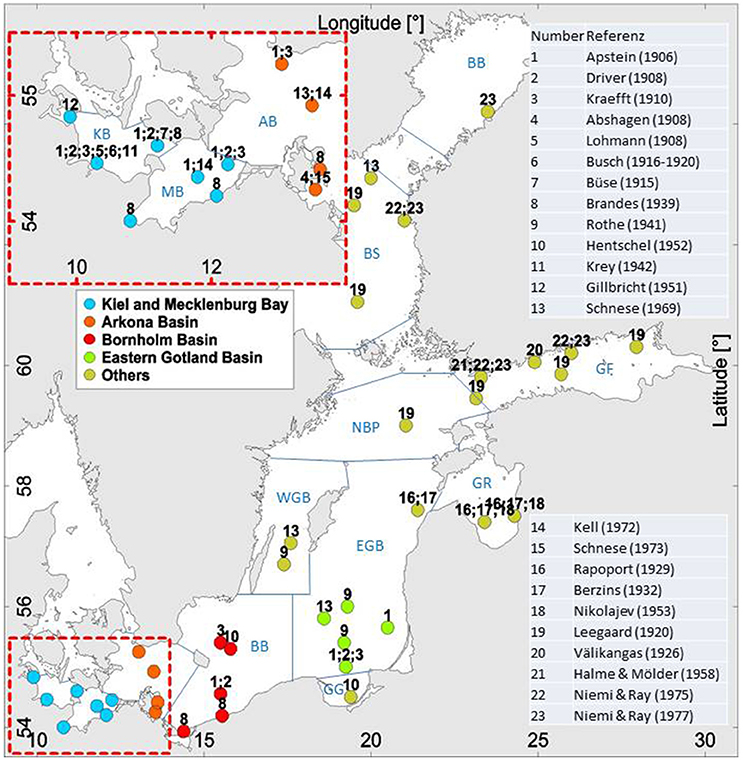
Figure 1. The Baltic Sea with its sub-regions: KB, Kiel Bay; MB, Mecklenburg Bay; AB, Arkona Basin; BB, Bornholm Basin; GG, Gulf of Gdańsk; EGB, Eastern Gotland Basin; WGB, Western Gotland Basin; NBP, Northern Baltic Proper; GR, Gulf of Riga; GF, Gulf of Finland; BS, Bothnian Sea; BB, Bothnian Bay. The numbers at the sampling locations relate to the references shown in the figure and listed in Table S1. The details of Kiel and Mecklenburg Bays (combined into KMB) as well as Arkona Basin are given in the inset.

In addition to the salinity gradient, there are north-south gradients in insolation, temperature, day length, and ice coverage. As these may influence the Dia/Dino index, the different Baltic regions, as defined by HELCOM (2016a) and based on geographic characteristics, must be evaluated separately.

The bottom of the Baltic Proper is morphologically structured into the Arkona, Bornholm, Eastern Gotland, and Western Gotland Basins, which increase in depth toward the central Baltic. North of the two Gotland basins, the Northern Baltic Proper forms a transitional region to the Gulfs of Bothnia and Finland. The Gulf of Riga is a widely separate water body lying between Latvia and Estonia whereas the Gulf of Gdańsk is open to the Baltic Proper.

Nutrient Analyses

Only nutrient data based on methods that were carefully checked and discussed by the originators have been considered in Section “Historical nutrient data.” The oldest usable silicate data from Kiel Bay were reported by Raben (1910), who used a method described by Raben (1905). Exactly 3 L of filtered water were acidified with hydrochloric acid and boiled down to dryness with several repetitions. After the last hot washing step, the precipitated amorphous silica was separated by filtration, combusted and weighed.

For the determination of both phosphate and silicate concentrations, the methods described by Atkins (1930) were applied by Wattenberg and Meyer (1936/1937) and those of Wattenberg (1937) were adopted by Krey (1942). Krey et al. (1978) determined phosphate but not silicate, still using the method of Wattenberg (1937). Both phosphate and silicate methods utilized molybdenum-sulfuric acid reagents and measured the emerging color in a photometer. The differentiation between the phosphate and silicate analysis is given by the reaction conditions, especially the pH.

In more recent investigations (Bodungen, 1975, and following studies), standard methods were employed which are still recommended in actual manuals (Grasshoff et al., 1999). The phosphate determination is based on modifications by Koroleff to the procedure of Murphy and Riley (1962), which uses two solutions instead of a single reagent; the first contains sulfuric acid, ammonium molybdate and antimony ions, and the second contains ascorbic acid. The blue color is measured in a photometer at 885 nm. The precision of the phosphate analysis under optimum conditions is 0.01 μM. The silicate determination is based on the formation of a yellow silicomolybdic acid which is reduced to intensely colored blue complexes which are measured by a photometer at 810 nm.

Phytoplankton Analyses

Early methods for the quantitative sampling of phytoplankton differed from those in use today. A general problem was enrichment of the samples for microscopy, which was solved in early studies by net sampling. However, the net mesh size was not well defined and small cells were more or less lost. The earliest “quantitative” plankton study was conducted by Hensen (1887), who collected samples from Kiel Bay between 1883 and 1886 using silk gauze (Müller gauze no. 20) with a mesh size of approximately 53 μm; this resulted in the loss of significant components of the phytoplankton community. Thus, the samples from March to May 1884 were described as mostly comprising large Coscinodiscus and Ceratium species, both of which were disproportionately enriched by the net. In addition, the reported abundances in spring were lower than those in autumn by a factor of nearly 1,000 and probably not reliable. In order to avoid misinterpretations, the data of Hensen (1887) were not considered in the present study. Nonetheless, a pioneering aspect of that early study was the introduction of quantitative counting using a precisely movable microscopic stage and a counting grid on the slide. This methodology was applied by many other researchers and considered “quantitative” despite the fact that net sampling generally is not.

Indeed, Lohmann (1908) pointed out the unsuitability of net sampling for quantitative analysis and instead used water samples enriched by filtration and centrifugation for microscopic analysis. This was the first complete analysis of phytoplankton, including nanoplankton, and the method was truly quantitative. Microscopic analyses of taxon abundance were performed according to the method of Hensen (1887). However, Lohmann (1908) additionally introduced the calculation of biovolume and carbon contents, based on stereometric formulas of geometric bodies that best approximate cell shapes, with typical lengths and widths for individual species. This was an important step because biovolume and the corresponding biomass are more important than abundance in understanding and modeling matter and energy fluxes in ecosystems.

The methodology of Lohmann (1908) for quantitative phytoplankton analysis was further developed by Utermöhl, beginning with special microscopy eyepieces for successive scanning of the sample in defined stripes (Utermöhl, 1927), an inverted microscope (Utermöhl, 1931b), and use of a single chamber for both sedimentation and counting of the sample (Utermöhl, 1931a), followed by the invention of the combined plate chamber, consisting of a cylindrical settling chamber and a baseplate (Utermöhl, 1958). The Utermöhl method is still the stipulated method for phytoplankton analysis in the HELCOM monitoring program (HELCOM, 2014).

Other studies of the early twentieth century neglected the biomass calculation and presented only abundance data. Although abundance data are not intended in the standard Dia/Dino index, they deliver valuable quantitative information on the phytoplankton dominance during the spring bloom and are therefore also used for the calculation of a Dia/Dino index if biomass data were lacking. If both the abundance-based and the biomass-based Dia/Dino indexes could be calculated, then the latter had priority and the former was neglected. Even semi-quantitative (i.e., biomass rankings) and qualitative (i.e., species lists) information may be of use. Therefore, papers providing only qualitative information were included in this study, although their results could not be used for calculations.

Taxonomic problems and difficulties in species identification do not influence the Dia/Dino index, because diatoms and dinoflagellates could be easily distinguished even in the early twentieth century.

The specific methods used in the different historical studies are briefly presented in Section “Quantitative phytoplankton studies” together with the associated data. Short information on samplings and analytical methods applied in the different studies is also given in Table S1.

Calculation Method

The Dia/Dino index is defined by the following formula (Wasmund et al., 2017):

$\begin{array}{l}\text{Dia}/\text{Dinoindex}={\text{BM}}_{\text{Dia}}/({\text{BM}}_{\text{Dia}}+{\text{BM}}_{\text{Dino}})\end{array}$

Seasonal averages of the biomass of planktonic diatoms (BM_Dia) have to be divided by the combined biomass of planktonic diatoms and autotrophic + mixotrophic dinoflagellates (BM_Dino). This leads to a simple absolute measure with values ranging from 0 to 1. If diatoms dominate, the value of the Dia/Dino index is >0.5; if autotrophic + mixotrophic dinoflagellates are dominant, the value of the index is <0.5.

Only spring bloom data are needed to calculate the Dia/Dino index. According to HELCOM (1996), the spring bloom in the Kattegat/Belt Sea, including Kiel Bay and Mecklenburg Bay, may occur any time between February and April, and in the Baltic Proper any time between March and May. The spring season is defined accordingly. This period from March to May also covers the spring bloom in the northern Baltic Proper (Höglander et al., 2004), Gulf of Finland (Niemi and Ray, 1977; Jaanus and Liiva, 1996), Gulf of Riga (Jurgensone et al., 2011), and Bothnian Sea (Andersson et al., 1996). In the Bothnian Bay, a spring bloom cannot be similarly distinguished because phytoplankton (diatom) growth typically starts later and reaches a peak usually only in June or July (Alasaarela, 1979).

Results

Historical Nutrient Data

Eutrophication is probably the most important anthropogenic pressure in the Baltic Sea. Together with the phytoplankton data, we made use also of the few historical nutrient data available in order to identify the period of most severe eutrophication. Sufficient data of a quality comparable to the recent data were only identified from Kiel Bay. For assessing the eutrophication, the winter nutrient concentrations are most relevant whereas for the phytoplankton, the annual mean biomass representing nearly the whole vegetation period in Kiel Bay is the most appropriate (Figure 2).

FIGURE 2

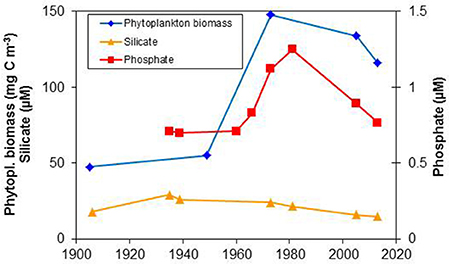
Figure 2. Trends in the late-winter concentrations of phosphate and silicate as well as mean annual phytoplankton biomass (in carbon units) in the upper mixed layer of Kiel Bay. Data sources are provided in the text.

The oldest usable silicate data from Kiel Bay were reported by Raben (1910), but phosphate data from the same author (Raben, 1916-1920) could not be used because of methodological problems and corresponding over-estimations. Wattenberg and Meyer (1936/1937) measured nutrient concentrations in the outer Kiel Fjord from 12 February 1935 to 16 February 1936. Their surface water data from the beginning and end of their time series, when the annual phosphate peaks occurred, are used in this study and are presented in Figure 2 as 2-year mean values. Krey (1942) performed comprehensive measurements in 1939. In a later study, Krey et al. (1978) took water from three stations in Kiel Bay, each represented by 6 sampling depths, and showed that late-winter phosphate concentrations were constant between 1958 and1960 but started to increase by 1965–1966. Silicate data were not reported. Phosphate concentrations continued to increase from 1972 to 1974, according to Bodungen (1975), while Grasshoff (unpubl., cited in Bodungen, 1986) determined peak values in 1980–1982. Monitoring data from 2000 to 2014, obtained from the State Agency for Agriculture, Environment and Rural Areas, are also included in Figure 2. For each year, the agency's February data from the different outer-coastal and open-water stations were combined. For equal-weighting of the historical with the recent data points in Figure 2, mean values for 2000–2009 and 2010–2014 are reported in the figure.

The nutrient data presented in Figure 2 were compared with mean annual phytoplankton biomass data from 1905 to 1906 (Lohmann, 1908), 1949 to 1950 (Gillbricht, 1951), 1972 to 1974 (Bodungen, 1975) and recent phytoplankton data from the monitoring program of the Leibniz Institute for Baltic Sea Research. Only phytoplankton data that were available in carbon units were considered in order to be able to include the valuable data of Lohmann (1908) which were only given as carbon. The annual mean values are covering the entire vegetation period which extends from February to December in Kiel Bay. The annual data were combined to yield decadal means from 2000–2009 to 2010–2016. The rough graph in Figure 2 shows a relationship between the phytoplankton trend and phosphate concentrations whereas there was no significant change in silicate concentrations. Based on these historical data, the trophic state appears to have been fairly constant until the end of the 1950s; thus, data until the end of the 1950s can be considered as the “historical” reference conditions.

Quantitative Phytoplankton studies

A compilation of historical phytoplankton data from 23 sources is presented in the Supplement as Table S1. It arranges the data according to regions, from west to east, and within regions in temporal order. The regional array could not be strictly followed if research cruises covered larger areas. The table starts with the oldest reliable and well-documented data and ends with data from 1973, when anthropogenic changes in the ecosystem became evident.

The publications used are numbered from 1 to 23 and the sampling locations of these studies are indicated by the same numbers in Figure 1. The corresponding reference is reported in the last column of Table S1. The sampling locations are specified in the second column of the table. Sampling stations located close to each other are combined to a single point in Figure 1. The number of stations and sampling dates is listed in the third column and the sampling periods in the fourth column. Only samples from the surface layer were considered, but in some cases those from deeper depths were included, especially when sampling was carried out by net hauls. Information on the sampling method is also provided in the table.

As only data on taxonomic groups are needed to calculate the Dia/Dino index, species-level data are not discussed herein. However, in a few cases the species information was useful. If the species names changed, the current synonyms were used and the name from the original paper was placed in parentheses in the text below. However, in the case of Skeletonema costatum the original name was retained because it was unclear which species was present in the historical samples after the revision of this genus by Sarno et al. (2005) and Zingone et al. (2005).

The results of regular cruises conducted within the framework of the ICES have only been published in part. On the German cruises, nets and the quantitative method of Hensen (1887) were applied. The first report from a monitoring cruise of this type (“Terminfahrt”) was that of Apstein (1906). From the data collected during four cruises in 1903, only data from the spring cruises (February and May) are presented because, as noted above, spring is defined herein as lasting from February to April in the Belt Sea (Kiel Bay and Mecklenburg Bay) and from March to May in the Baltic Proper. In 1903, however, the major spring bloom (Chaetoceros spp.) in Kiel Bay occurred much later, in early May. Moreover, the relatively high abundance of Ceratium species in February in the Belt Sea was surprising and probably represented overwintering stages of the preceding autumn bloom, as this genus is currently not known to be common in February.

Driver (1908) reported on the German cruises of 1905, during which the method of Apstein (1906) was used. The long net hauls resulted in the inclusion of deeper layers, resulting in dilution effects and therefore abundance data that were lower than expected. Similar to Apstein (1906), also Driver (1908) found the biomass maxima in May. Therefore, we included exceptionally their data from May in the calculation of the Dia/Dino index of Kiel Bay and Mecklenburg Bay.

The cruise reported on by Kraefft (1910) was conducted at the end of March 1906 and one station per sea area was sampled. Only the data from the vertical surface haul (0–5 m) are included in the present study.

A higher seasonal coverage was possible in coastal waters because of easier access to the sampling stations. Abshagen (1908) undertook semi-quantitative investigations (4-grade scale) in Greifswald Bodden from 1900 to 1901 and from 1904 to 1908 as well as quantitative investigations from 1900 to 1908. The quantitative data are of particular interest even though they are limited to abundance data from two sampling dates in spring. The samples were taken by a vertical net haul from the sea bottom to the surface.

High-frequency investigations were carried out by Lohmann (1908) from April 1905 to August 1906 at Laboe station, located in the mouth of Kiel Fjord. Of the 27 samplings in 1905 and 33 samplings in 1906, however, only one sampling date was in the spring (February to April) of 1905. Nonetheless, it captured the spring bloom, which was almost exclusively composed of Chaetoceros spp. In 1906, the bloom peaked on almost the same date (11 April 1906, diatom abundance 2.0 × 10⁶ cells/L). This bloom was also dominated by Chaetoceros but S. costatum, Thalassiosira spp., and Thalassionema nitzschioides were present as well. The dominating dinoflagellates were small colorless Gymnodinium spp., which were not included in the study of Wasmund et al. (2017) because heterotrophic species were, as far as possible, excluded. The procedure followed by Lohmann readily allowed the calculation of biomass (Table S1). The value for 1905 represents only the bloom peak, from a single measurement and is therefore higher than the value for 1906, which is the mean of 12 values including those from the peak and from the pre- and post-bloom stages, when biomass is much lower. Details on the data of Lohmann (1908) can be found in Wasmund et al. (2008).

Busch (1916-1920) investigated the same station as Lohmann (1908). The high sampling frequency from 1 March 1912 to 10 May 1913 covered two spring periods. In contrast to Lohmann (1908), net sampling was carried out by means of the medium Apstein net (silk gauze no. 20) and the whole water column was sampled. The spring bloom of 1912 was sampled only on 1 March, 3 April, and 24 April. The dominant genus was Chaetoceros; the maximum of 100,000 cells/L was detected on 3 April 1912. The spring bloom in 1913 peaked on 7 March (Chaetoceros spp.: 475,000 cells/L, S. costatum: 157,000 cells/L) and declined until 23 April (Chaetoceros spp.: 112,000 cells/L, S. costatum: 276,000 cells/L).

Büse (1915) followed a strategy similar to that of Busch (1916-1920). Because the investigation period extended from 3 January 1910 to 27 March 1911, two spring periods were covered, at least in part. The fixed station in that study was a lightship positioned in the Fehmarnbelt between Kiel Bay and Mecklenburg Bay. The peak of the Chaetoceros bloom occurred at the end of March, with up to 636 × 10⁶ cells/m² in the 26-m deep water column, accompanied by 164 × 10⁶ T. nitzschioides cells/m² on 28 March 1910 and 4.2 × 10⁹ S. costatum cells/m² on 27 March 1911.

After a long gap due to World War I and the recession-plagued post-war period, German cruises and coastal samplings finally resumed (Brandes, 1939). However, from the data collected during this period, only those from the spring 1937 campaign were quantitative and thus suitable for this study. Sampling during the 1937 campaign was conducted at different fixed stations, including the Lightship Fehmarnbelt and five coastal stations, with 1-L water samples filtered through a 40-μm mesh. This procedure allowed a more precise determination of the sample volume than achieved by direct net hauls. The time-series from that campaign revealed that the maximum of the spring bloom occurred on 18 March 1937 at the Fehmarn Belt station and from the end of March to the beginning of April at the eastern stations. All of these blooms were dominated by Chaetoceros spp. and S. costatum. Data from a cruise conducted at the end of March 1938 had to be excluded because the dominant Chaetoceros and Skeletonema were not counted.

Samples from a cruise in late March 1938 were quantitatively analyzed by Rothe (1941). A water sampler was used to collect samples from a series of depths and a defined volume was filtered through a sieve of 40-μm mesh size. Only data from the 0 and 20 m depths were used in the calculations shown in Table S1. The numerous stations were grouped into four sea areas; the averaged positions, represented by a single point, are shown in Figure 1.

Hentschel (1952) applied the same method as Brandes (1939), reporting on four cruises conducted between the islands of Bornholm and Öland. Only data from the spring cruise of March 1938 were of interest in the present study. Rather than differentiating between the 27 stations, mean values from the respective data were calculated. The diatom S. costatum clearly dominated, accounting for >50% of the abundance at all stations. Dinoflagellates, dominated by Peridiniella catenata (Peridinium catenatum), were of secondary importance.

Krey (1942) conducted weekly samplings from 13 March to 27 November 1939 at Laboe station, the same station investigated by Lohmann (1908) and Busch (1916-1920). A 3- to 5-L volume of sampled water was filtered through a sieve (“Kolkwitzsieb”) of 80-μm mesh size and phytoplankton were counted using an inverted microscope according to the method of Utermöhl (1931b). Both abundance and biovolume, which can easily be converted into biomass (wet weight), were determined (Table S1).

Gillbricht (1951) investigated a fixed station at the mouth of Flensburg Fjord from June 1949 to June 1950. The spring campaign comprised six samplings, conducted from 19 March to 30 March 1950. At each one, 12 samples were collected from a series of depths at 2.5-m intervals. In the present study, the mean values of samples from all sampling depths and dates were calculated in order to concentrate the numerous data to a single value. Gillbricht (1951) was among the first to take full advantage of the Utermöhl method, using whole water samples such that organisms in the small size fraction were retained. Abundance and biomass (cytoplasm) were calculated as suggested by Lohmann (1908).

More recent (April and May 1967) investigations in the Baltic Proper and the Gulf of Bothnia (5 stations) were conducted by Schnese (1969). Water samples were obtained from different depths and analyzed quantitatively for phytoplankton biomass using the method of Utermöhl (1958). In the present study, biomass data were calculated from the abundance data because cell volumes were provided in the published paper. The Dia/Dino indexes were always high, except in the southern sector of the Eastern Gotland Basin (station 4c), which was sampled relatively late (15 May 1967), after the Skeletonema bloom. Therefore, this single value was not considered to be representative of the spring bloom.

Phytoplankton samples from monitoring cruises conducted from March 1968 to February 1971 were analyzed by Kell (1972), based on the method of Utermöhl (1958). For the purpose of the present study, biomass data were extracted from the graphs, which already included the mean values of data obtained from all stations in Mecklenburg Bay and the Arkona Basin. The biomass data show that the spring bloom was not met in 1968 and 1969, but in 1970. The spring bloom of March 1970 was composed almost entirely of diatoms. Centrales dominated but there was also a large share (35%) of Pennales (Pauliella taeniata). In May, when the bloom biomass had declined, the pennate diatom Diatoma tenuis (Diatoma elongatum) gained relative dominance in the southeastern part of Arkona Basin.

In the Greifswald Bodden, the early study of Abshagen (1908) was followed much later by that of Schnese (1973). Water samples collected from a depth of 1 m and from 1 m above the bottom were used in quantitative phytoplankton analyses according to the method of Utermöhl (1958).

The spring phytoplankton of the Gulf of Riga and the Latvian coastal waters of the Baltic Sea were quantitatively investigated for the first time in 1925 by Rapoport (1929). Surface water (25 L) was filtered through a mesh (Müller gauze no. 20), the filtrate diluted to 50 mL, and a sub-sample of 1 mL counted in a Kolkwitz chamber. The spring season was well-represented, as data were available for every month (March–May). For clarity, the 16 stations have been aggregated into three groups: (i) Latvian coastal waters from Liepaja to the Irbe Strait, (ii) southwestern Gulf of Riga from Cape Kolkasrags to the mouth of the Daugava River, and (iii) eastern coast of the Gulf of Riga. Rapoport (1929) presented abundance data based on a 100-L water sample, but they may be biased by a calculation error, as the abundances are much lower than expected. Since the Dia/Dino index is a relative measure, it is not influenced by constant abundance or biomass errors. Nevertheless, in Table S1 the values determined by Rapoport (1929) have been multiplied by a factor of 1,000 in order to shift them into a realistic range. Diatoms such as Actinocyclus octonarius (Actinocyclus ehrenbergii) and Thalassisira baltica were clearly dominant compared with the dinoflagellate P. catenata (P. catenatum). Only in the southeastern part of the studied area was P. catenata more abundant, which lowered the Dia/Dino index.

Quantitative data on phytoplankton abundance in the Gulf of Riga and Latvian waters, between Ventspils and Cape Kolkasrags (16 stations), from May 1928 were presented by Berzins (1932). Surface samples were gathered by the filtration of 25 L of surface water; deeper hauls were realized using a medium Apstein net. The samples were prepared as a dilution range and counted in Kolkwitz chambers. Only net samples from 0 to 20 m were taken into account. Again, for clarity, data from the stations were aggregated. In contrast to Rapoport (1929), Berzins (1932) found the highest share of P. catenata (Gonyaulax catenatum) at one coastal station (station 8) of the Baltic Proper whereas the abundance of this species was very low in the eastern Gulf of Riga.

The biomass data of Nikolajev (1953), from samples collected in the southern and eastern Gulf of Riga in spring 1947, are sparse and the method was not sufficiently described. Nevertheless, a Dia/Dino index could be calculated and the data are included in Table S1. In a later study, Nikolajev (1957) reported on clear diatom dominance in March and May 1947.

Early phytoplankton abundance data from the Gulfs of Finland and Bothnia and the Northern Baltic Proper (6 stations) were published by Leegaard (1920). However, station F61 was excluded in the present study because there were no data on P. catenata (Gonyaulax catenata), despite its documented occurrence. The data may not be representative of the spring because each station was sampled only once, in May 1912, but they are valuable because they are based on whole water samples enriched by centrifugation and quantified by cell counting. Seven to ten separate samples were taken from each depth profile, but only the four samples representing the upper 20 m were included in the calculations presented herein. The most abundant diatom was P. taeniata (Achnanthes taeniata), and the most abundant dinoflagellate P. catenata. Diatoms were overwhelming in the gulfs, leading to high Dia/Dino indexes, if based on the reported abundance data given. The Dia/Dino index from the Northern Baltic Proper (station F74) was much lower. This may be atypical because P. taeniata was detected as resting spores and at greater depth (30 m), indicating that the sampling date was too late to capture the diatom spring bloom.

Quantitative data from the Helsinki region (13 stations) from 7 to 8 May 1919 were reported by Välikangas (1926). Surface water (50 L) collected by a bucket was filtered through a net (Müller gauze no. 20). Net hauls were taken already on 7–9 April 1919, during ice coverage at some stations. Rough semi-quantitative estimates revealed the start of a P. taeniata (A. taeniata) bloom such that by 7–8 May 1919 a diatom-Peridiniella association was fully developed.

The Pojo Bight, in the western Gulf of Finland, was investigated by Halme and Mölder (1958) from June 1936 to May 1937. Only stations in the marine region (sea areas MI–MIV) are considered in the present study. Samples collected during the spring cruises in March, the beginning of May, and the end of May 1937 were quantitatively analyzed using the Utermöhl method, but only the abundances of the “predominants” were reported. Diatoms abundances were consistently high, but data on dinoflagellates [P. catenata (G. catenata)] were mentioned only from the beginning of May 1937.

Although the data of Niemi and Ray (1975, 1977), based on studies conducted in 1972 and 1973, respectively, may not be considered as historical, they are presented here as a link to recent investigations. Stations in the Gulfs of Finland and Bothnia, still considered as “undisturbed” at that time, were sampled at 0.2, 2, 4, 6, 8, 10, 15, and 20 m depths, but only the data from the 0- to 10-m samples are considered herein. Counting was performed by the Utermöhl technique and the biovolumes were calculated based on geometric formulas. Because neither publication presented the original data, a direct calculation of the Dia/Dino index was not possible. However, relative biomass information could be extracted from the bar graphs and related to the total biomass given in the line graphs. Maxima of phytoplankton biomass occurred in April–May, which confirms our strategy to consider samples from March to May as spring samples also in this northern water.

Non-quantitative Phytoplankton Studies

While, for the purpose of the present study, non-quantitative data were of less value than the quantitative data, they nevertheless provided useful information on the diatom/dinoflagellate ratio in spring blooms. Thus, the present study includes also historical literature that was descriptive and contained species lists without quantification.

A semi-quantitative method, as suggested by the ICES, was applied by Fraude (1906) in 1905 in the Greifswald Bodden (German coast). The occurring species were assigned to a four-grade scale. A massive occurrence was reported for Chaetoceros species and to lesser degrees also for Coscinodiscus radiatus from 16 February to 26 March 1905 and for S. costatum from 18 May to 28 May 1905 whereas dinoflagellates were rare.

Wattenberg and Meyer (1936/1937) used a quantitative method (the Kolkwitzsieb and Utermöhl method, later also applied by Krey, 1942; see above) but did not present their data, only selected figures. Thus, all that is known is that the spring bloom in the Kiel Bay in 1935 started at the beginning of March and was characterized by strong diatom growth whereas dinoflagellates (Ceratium) were rare.

Bandel (1940) investigated six stations located in front of Warnemünde, eastern Mecklenburg Bay, once per month from April 1937 to May 1938. Larger organisms were collected in net hauls, taken with the closing net no. 20 and smaller organisms via water samples followed by enrichment in a centrifugation step. Because the data of the quantitative analyses were not presented in that paper, the results are considered to be descriptive. Nevertheless, a large Chaetoceros bloom clearly occurred in April 1938, during which time dinoflagellates were insignificant.

The dominating phytoplankton species in the Kaliningrad region (Russia) from January to December 1935 were described by Sommer (1936). The spring bloom was formed mainly by P. taeniata (Achnanthes taeniata) whereas dinoflagellates [P. catenata (Gonyaulax catenata)] were of minor importance. The occurrence of the spring bloom in this area from March to May, dominated by diatoms, was confirmed by Schmidt-Ries (1939).

In the Gulf of Riga, a diatom-dominant spring bloom was still typical in the late 1960s and 1970s (Rudzroga, 1974; Kalveka, 1980) but data relevant to the present study were not presented by the authors. Jurgensone et al. (2011) provided monthly mean percentages for the various phytoplankton groups between 1976 and 2008 and found still general diatom dominance during the spring bloom (April–May).

Hessle and Vallin (1934) concentrated on zooplankton, presenting semi-quantitative springtime phytoplankton data only from a few stations near the Swedish coast. Because of the relatively large mesh width of the net used in that study, small phytoplankton were not adequately represented. Chaetoceros species and P. taeniata (Achnanthes taeniata) were marked as “common” in the spring of 1926 at coastal stations located at 57.7°–57.9°N, but P. catenata (Gonyaulax catenata) was only marked as “present.”

Trends in the Dia/Dino index

The Dia/Dino indexes calculated in Table S1 are depicted in Figure 3. They are specified for selected regions, but regions with lower data coverage (Western Gotland Basin, Northern Baltic Proper, Gulfs of Gdańsk, Riga, Finland, and Bothnia) were combined as “Others.” Annual data from several stations within the same regions were collapsed to a single point. Both historical and recent data are shown. The latter originated from the HELCOM monitoring program, which started in 1979, and are stored in the ICES data bank. As the “Other” regions are highly different and would overload and blur the image, we selected only the Northern Baltic Proper from the “Other” recent data for presentation in Figure 3.

FIGURE 3

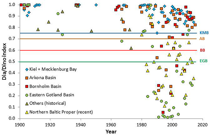
Figure 3. Summary of the historical and recent Dia/Dino indexes in different areas of the Baltic Sea since 1901. Suggested GES thresholds for Kiel Bay and Mecklenburg Bay (KMB), Arkona Basin (AB), Bornholm Basin (BB), and Eastern Gotland Basin (EGB) are plotted as lines.

Discussion

A comparison of historical and recent data revealed a clear trend even without statistical evaluation. Diatom dominance, i.e., a Dia/Dino index >0.5, occurred in all studied areas of the Baltic until 1983. The exceptionally low Dia/Dino index values in the Eastern Gotland Basin in 1984 and 1988 and the relatively low values in the Northern Baltic Proper in 1983/1984 were followed by abrupt decreases in every considered area between 1989 and 1991. The disappearance of diatoms and their replacement by dinoflagellates was discussed by Wasmund et al. (1998, 2013) and Alheit et al. (2005).

The focus of this study is the historical data, as they form the basis for the definition of GES. Thus far, GES thresholds have been set according to monitoring data starting in 1979. Derivation of GES thresholds is explained in Wasmund et al. (2017). For Kiel Bay and Mecklenburg Bay, the threshold Dia/Dino index value was set at 0.75, and for the Eastern Gotland Basin at 0.5 by Wasmund et al. (2017). These values are plotted as a line in Figure 3. Using the same strategy, Wasmund et al. (2016) suggested Dia/Dino GES thresholds for the Arkona and Bornholm Basins of 0.7 and 0.6, respectively. These GES thresholds have already been accepted by HELCOM (2016b).

However, the 1980s were already characterized by elevated rates of eutrophication and therefore inappropriate as a reference state (see Figure 2). Thus, the present study used historical data originating from the pre-eutrophication period, which according to the reliable data consistently revealed high Dia/Dino indexes. The Dia/Dino index of 0.41 in 1912 (Northern Baltic Proper) is unrealistic because it was based on very late sampling (16 May 1912) such that the diatom bloom, which generally occurs earlier, was most likely missed. Nevertheless, this outlier was kept in the calculation of the annual mean value of 1912 as part of the “Other” areas. The less reliable data have also been retained in Table S1 and in the calculations used for Figure 3, to avoid the subjective exclusion of data. The lower representativeness of data obtained from only one sampling occasion vs. data that derive from higher sampling frequencies should be kept in mind by the reader.

As pointed out above, abundance data were used if biomass data were not available, but the standard Dia/Dino index requires the latter. In a few cases (Lohmann, 1908; Krey, 1942; Gillbricht, 1951; Schnese, 1969), both abundance and biomass data were given (Table S1). Using those data, the mean Dia/Dino indexes based on abundance and biomass were 0.99 and 0.88, respectively. Theoretically, all Dia/Dino indexes based on abundance would have to be corrected by a conversion factor of 0.89 (=0.88/0.99). However, because this factor was not well-founded, the conversion was omitted. As seen in Figure 3, even when the conversion factor was applied, the historical Dia/Dino indexes were well above the GES threshold of 0.5. The recent monitoring data (since 1979) are generally reported as biomass.

The temporal mismatch between the increase in eutrophication (in the 1960s; Figure 2) and the decrease in the Dia/Dino index (in the late 1980s; Figure 3) suggests that the index is not primarily an indicator of eutrophication. According to Wasmund et al. (1998, 2013), the magnitude of the diatom bloom is controlled by the minimum winter temperature. This conclusion is supported by Kononen and Niemi (1984) and Klais et al. (2013), who reported diatom dominance after a late (April) break-up of the ice and dinoflagellate dominance after an early (March) break-up of the ice. Ice cover is, however, generally rare in the southern Baltic Proper, where the strongest phytoplankton changes occurred, and cannot be the causative factor there. The effect of temperature on phytoplankton composition, including that via the food web, is discussed by Wasmund et al. (2013).

Another problem to be solved before a Dia/Dino-index-based GES could be suggested was the possibility of long-term oscillations in the historical indexes, which would have complicated the establishment of reference conditions. However, our results do not show any indication of fluctuations in the Dia/Dino indexes (Figure 3). Even in the case of gaps, such as occurred between 1950 and 1963, the historical Dia/Dino indexes were presumably high and stable. They were not influenced by the sporadic changes in salinity that are caused by mayor inflows of salt water from the North Sea (Matthäus et al., 2008; Mohrholz et al., 2015) or other fluctuating factors.

A by-product of our research was phenological information. Hensen (1887), Apstein (1906), and Driver (1908) found relatively high Ceratium abundances still in February and March which were remnants of the preceding autumn bloom. This dinoflagellate disturbs the Dia/Dino index because it does not belong to the spring bloom. The problem appears only in the Belt Sea, as Ceratium does not occur in the Baltic Proper. The historical spring blooms in Kiel Bay started later (in March) than is currently the case (now frequently in February), reaching peaks only in May. Thus, the historical spring period may have ranged from March to May whereas spring in the Belt Sea has more recently begun in February and ended in April. Setting the historical spring in the Belt Sea between March and May resolves the Ceratium problem and removes the relatively low historical Dia/Dino indexes from February, as seen in the data of Apstein (1906) and Driver (1908). If based on the period from March to May the historical Dia/Dino indexes in Kiel Bay would always be high (>0.94).

Conclusions

Thanks to the availability of historical phytoplankton data, historical Dia/Dino indexes could be calculated, that were used for suggesting GES thresholds for that indicator. During the spring blooms in all regions tested until 1973, diatoms consistently dominated over dinoflagellates, such that the Dia/Dino index was consistently >0.5. Oscillations in the historical Dia/Dino indexes did not occur. However, recent monitoring data have revealed a sudden decrease, especially between 1984 and 1991. This decline in the Dia/Dino index indicates a worsening of the environmental status related not to eutrophication but to warmer winters. The decrease in the proportion of diatoms and the increase in that of dinoflagellates may have consequences for the food web.

Our study also confirmed previously approved GES thresholds for Kiel and Mecklenburg Bays as well as for the Arkona, Bornholm, and Eastern Gotland Basins. For the “Other” regions in the Baltic Sea, for which GES thresholds are still lacking, the historical data compiled in this study may support the authorities who are responsible for the fixing of GES thresholds in their areas, thereby making the Dia/Dino index fully operational.

Summarizing the phenological results, we may conclude at least from Kiel Bay that the spring bloom period shifted from March-May in the early twentieth century to February-April in recent times.

Author Contributions

NW collected the historical data from literature and recent data from contributions of co-authors to the related paper (Wasmund et al., 2017); he compiled and evaluated the data, and wrote the manuscript.

Conflict of Interest Statement

The author declares that the research was conducted in the absence of any commercial or financial relationships that could be construed as a potential conflict of interest.

Acknowledgments

The monitoring data of HELCOM were provided by the ICES data bank. We are grateful to the recent data contributors Susanne Busch and Jeanette Göbel (Germany), Helena Höglander and Marie Johansen (Sweden), Andres Jaanus (Estonia), and Janina Kownacka (Poland). Recent nutrient data of the State Agency for Agriculture, Environment and Rural Areas, Flintbek, from Kiel Bay were contributed by Jeanette Göbel. My colleague Jan Donath produced Figure 1.

Supplementary Material

The Supplementary Material for this article can be found online at: https://www.frontiersin.org/article/10.3389/fmars.2017.00153/full#supplementary-material

Table S1. Compilation of historical phytoplankton data from the Baltic Sea. The references, given in the last column and numbered from 1 to 23, relate to the numbering in Figure 1. The combined data from each spring season and sea area are shown in separate lines. The mean abundance and biomass values of diatoms and dinoflagellates are given as they provided the basis for calculations of the Dia/Dino indexes.

References

Abshagen, G. (1908). Das Phytoplankton des Greifswalder Boddens. Dissertation, Greifswald.

Alasaarela, E. (1979). Phytoplankton and environmental conditions in central and coastal areas of the Bothnian Bay. Ann. Bot. Fennici. 16, 241–274.

Google Scholar

Alheit, J., Möllmann, C., Dutz, J., Kornilovs, G., Loewe, P., Mohrholz, V., et al. (2005). Synchronous ecological regime shifts in the central Baltic and the North Sea in the late 1980s. ICES J. Marine Sci. 62, 1205–1215. doi: 10.1016/j.icesjms.2005.04.024

CrossRef Full Text | Google Scholar

Andersen, J. H., Carstensen, J., Conley, D. J., Dromph, K., Fleming-Lehtinen, V., Gustafsson, B. G., et al. (2015). Long-term temporal and spatial trends in eutrophication status of the Baltic Sea. Biol. Rev. 92, 135–149. doi: 10.1111/brv.12221

PubMed Abstract | CrossRef Full Text | Google Scholar

Andersson, A., Hajdu, S., Haecky, P., Kuparinen, J., and Wikner, J. (1996). Succession and growth limitation of phytoplankton in the Gulf of Bothnia (Baltic Sea). Marine Biol. 126, 791–801. doi: 10.1007/BF00351346

CrossRef Full Text | Google Scholar

Apstein, C. (1906). Plankton in Nord- und Ostsee auf den deutschen Terminfahrten. 1. Teil (Volumina 1903). Wissenschaftliche Meeresuntersuchungen. Neue Folge, Abt. Kiel 9, 1–26.

Atkins, W.R. G. (1930). Seasonal variations in the phosphate and silicate content of sea-water in relation to the phytoplankton crop. Part, V. November 1927 to April 1929, compared with earlier years from 1923. J. Marine Biol. Assoc. 16, 821–852.

Google Scholar

Bandel, W. (1940). Phytoplankton- und Nährstoffgehalt der Ostsee im Gebiet der Darsser Schwelle. Int. Rev. Gesamten Hydrobiol. Hydrogr. 40, 249–304. doi: 10.1002/iroh.19400400303

CrossRef Full Text | Google Scholar

Berzins, B. V. A. (1932). Das Plankton der lettischen Terminfahrt im Frühjahr 1928 (Rigascher Meerbusen und Baltisches Meer). Folia Zool. Hydrobiol. 4, 68–102.

Bodungen, B. V. (1975). Der Jahresgang der Nährsalze und der Primärproduktion des Planktons in der Kieler Bucht unter Berücksichtigung der Hydrographie. Ph.D Thesis, Kiel University.

Bodungen, B. V. (1986). Annual cycles of nutrients in a shallow inshore area, Kiel Bight. - Variability and trends. Ophelia 26, 91–107. doi: 10.1080/00785326.1986.10421981

CrossRef Full Text | Google Scholar

Brandes, C.-H. (1939). Über die räumlichen und zeitlichen Unterschiede in der Zusammensetzung des Ostseeplanktons. Mitteilung aus dem Hamburgischen Zoologischen Museum und Institut 48, 1–47.

Brandt, K. (1897). Die Fauna der Ostsee, insbesondere die der Kieler Bucht. Verhandlungen der Deutschen Zoologischen Gesellschaft 7, 10–34.

Busch, W. (1916-1920). Über das Plankton der Kieler Föhrde im Jahre 1912/13. Wissenschaftliche Meeresuntersuchungen Neue Folge Abt. Kiel. 18, 25–142.

Büse, T. (1915). Quantitative Untersuchungen von Planktonfängen des Feuerschiffes “Fehmarnbelt” vom April 1910 bis März 1911. Wissenschaftliche Meeresuntersuchungen Neue Folge Abt. Kiel. 17, 229–280.

Driver, H. (1908). Das Ostseeplankton der 4 deutschen Terminfahrten im Jahre 1905. Wissenschaftliche Meeresuntersuchungen Neue Folge Abt. Kiel. 10, 106–127.

Elmgren, R., and Larsson, U. (2001). “Eutrophication in the Baltic Sea area: integrated coastal management issues,” in Science and Integrated Coastal Management, eds B. V. Bodungen and R. Turner (Berlin: Dahlem University), 15–35.

European Commission (2000). Directive 2000/60/EC of the European Parliament and of the Council establishing a framework for the Community action in the field of water policy, Legislative Acts and other instruments (ENV221 CODEC 513). Available online at: http://www.europarl.europa.eu/sides/getDoc.do?pubRef=-//EP//NONSGML+JOINT-TEXT+C5-2000-0347+0+DOC+PDF+V0//EN&language=SK

European Commission (2008). “Directive 2008/56/EC of the European Parliament and of the Council of 17 June 2008, establishing a framework for community action in the field of marine environmental policy (Marine Strategy Framework Directive),” in Official Journal of the European Union, L 164, 19-40. Available online at: http://eur-lex.europa.eu/legal-content/EN/TXT/PDF/?uri=CELEX:32008L0056&rid=1

European Commission (2010). “Commission Decision of 1 September 2010 on criteria and methodological standards on good environmental status of marine waters (notified under document C(2010) 5956), 2010/477/EU” in Official Journal of the European Union L 232/14. Available online at: http://publications.europa.eu/en/publication-detail/-/publication/a8eee6d0-6136-4dae-a2da-2c4334f144f7/language-en/format-PDF

European Commission (2015). Review of the GES Decision 2010/477/EU and MSFD Annex III – Cross-Cutting Issues (Version 4). GES_13-2015-02. Available online at: https://circabc.europa.eu/d/a/workspace/SpacesStore/53b2e4e2-2921-468a-941f-499811ee12f9/GES_13-2015-02_GESDecisionReview_Cross-cuttingIssues_v4.doc

Fraude, H. P. A. (1906). Grund- und Plankton-Algen der Ostsee. X. Jahresbericht der Geographischen Gesellschaft zu Greifswald 10, 223–350.

Gillbricht, M. (1951). Produktionsbiologische Untersuchungen in der Kieler Bucht. Kiel: University of Kiel.

Grasshoff, K., Kremling, K., and Ehrhardt, M. (eds.). (1999). Methods of Seawater Analysis, 3rd Edn. Weinheim: Wiley-VCH.

Hällfors, H., Backer, H., Leppänen, J.-M., Hällfors, S., Hällfors, G., and Kuosa, H. (2013). The northern Baltic Sea phytoplankton communities in 1903-1911 and 1993-2005: a comparison of historical and modern species data. Hydrobiologia 707, 109–133. doi: 10.1007/s10750-012-1414-4

CrossRef Full Text | Google Scholar

Halme, E., and Mölder, K. (1958). Planktologische Untersuchungen in der Pojo-Bucht und angrenzenden Gewässern. III. Phytoplankton. Ann. Bot. Societ. Zool. Bot. Fenni. Vanamo 30, 1–71.

Heiskanen, A.-S., Gromisz, S., Jaanus, A., Kauppila, P., Purina, I., Sagert, S., et al. (2005). Developing Reference Conditions for Phytoplankton in the Baltic Coastal Waters. Part I: Applicability of Historical and Long-Term Datasets for Reconstruction of Past Phytoplankton Conditions. Technical report, EUR 21582/EN/1, Joint Research Centre (JRC).

HELCOM (1996). Third periodic assessment of the state of the marine environment of the Baltic Sea, 1989-1993; background document. Balt. Sea Environ. Proc. 64:252.

HELCOM (2013). HELCOM core indicators. Final report of the HELCOM CORESET project. Baltic Sea Environ. Proc. 136, 1–74.

HELCOM (2014). Manual for Marine Monitoring in the COMBINE Programme of HELCOM. Available online at: http://www.helcom.fi/Documents/Action%20areas/Monitoring%20and%20assessment/Manuals%20and%20Guidelines/Manual%20for%20Marine%20Monitoring%20in%20the%20COMBINE%20Programme%20of%20HELCOM.pdf

HELCOM (2016a). Baltic Sea Environmental Status Map Service - Sea Environmental Monitoring - Assessment Units - HELCOM Subbasin Division Lines. Available online at: http://maps.helcom.fi/website/SeaEnvironmentalStatus/index.html

HELCOM (2016b). Outcome of the Fifth Meeting of the Working Group on the State of the Environment and Nature Conservation (State & Conservation 5-2016). Available online at: https://portal.helcom.fi/meetings/STATE%20-%20CONSERVATION%205-2016-363/MeetingDocuments/Final%20Outcome%20State%20and%20Conservation%205-2016.pdf

Hensen, V. (1887). Ueber die Bestimmung des Plankton's oder des im Meere treibenden Materials an Pflanzen und Thieren. 5. Bericht d. Kommission z. Wiss. Untersuch. d. deutschen Meere, Kiel. Jg. 12–16, 1–108.

Hentschel, E. (1952). Untersuchungen über das Plankton des Bornholmbeckens. Ber. Dtsch. Wiss. Komm. Meeresforsch. 12, 215–315.

Hessle, C., and Vallin, S. (1934). Undersökningar över plankton och dess växlingar i Östersjön under aren 1925-1927. (Investigations of plankton and its fluctuations in the Baltic during the years 1925-1927). (Swedish with English summary). Svenska Hydrografisk Biologiska Kommissionens Skrifter. Ny Serie. Biol. 1, 1–137.

Höglander, H., Karlson, B., Johansen, M., Walve, J., and Andersson, A. (2013). Overview of Coastal Phytoplankton Indicators and their Potential Use in Swedish Waters. Deliverable 3.3.-1. WATERS Report no. 2013:5. Havsmiljöinstitutet.

Höglander, H., Larsson, U., and Hajdu, S. (2004). Vertical distribution and settling of spring phytoplankton in the offshore NW Baltic Sea proper. Mar. Ecol. Prog. Ser. 283, 15–27. doi: 10.3354/meps283015

CrossRef Full Text | Google Scholar

Jaanus, A., and Liiva, K. (1996). A review of the phytoplankton monitoring data in the southern Gulf of Finland and an attempt at biogeographical grouping on these grounds. Proc. Estonian Acad. Sci. Ecol. 6, 57–72.

Jurgensone, I., Carstensen, J., Ikainiece, A., and Kalveka, B. (2011). Long-term changes and controlling factors of phytoplankton community in the Gulf of Riga (Baltic Sea). Estuar. Coasts 34, 1205–1219. doi: 10.1007/s12237-011-9402-x

CrossRef Full Text | Google Scholar

Kalveka, B. J. (1980). “On the seasonal cycles of phytoplankton development in the open part of the Baltic and in the Gulf of Riga in 1976. (in Russian),” in Proceedings of the Fisheries Research in the Baltic Sea, eds L. M. Vail, E. M. Kostrichkina, M. N. Lishev, E. M. Malokova, V. I. Pechatina, M. P. Poljakov, et al. (Riga), 36–45.

Kell, V. (1972). Phytoplanktonuntersuchungen in der Ostsee von der Lübecker Bucht bis zur Arkonasee. PhD thesis, Rostock.

Klais, R., Tamminen, T., Kremp, A., Spilling, K., An, B. W., Hajdu, S., et al. (2013). Spring phytoplankton communities shaped by interannual weather variability and dispersal limitation: mechanisms of climate change effects on key coastal primary producers. Limnol. Oceanogr. 58, 753–762. doi: 10.4319/lo.2013.58.2.0753

CrossRef Full Text | Google Scholar

Klais, R., Tamminen, T., Kremp, A., Spilling, K., and Olli, K. (2011). Decadal-Scale Changes of Dinoflagellates and Diatoms in the Anomalous Baltic Sea Spring Bloom. PLoS ONE 6:e21567. doi: 10.1371/journal.pone.0021567

PubMed Abstract | CrossRef Full Text | Google Scholar

Kononen, K., and Niemi, A. (1984). Long-term variation of the phytoplankton composition at the entrance to the Gulf of Finland. Ophelia (Suppl.) 3, 101–110.

Kraefft, F. (1910). Über das Plankton in Ost- und Nordsee und den Verbindungsgebieten mit besonderer Berücksichtigung der Copepoden. Wissenschaftliche Meeresuntersuchungen Neue Folge Abt. Kiel. 11, 29–108.

Krey, J. (1942). Nährstoff- und Chlorophylluntersuchungen in der Kieler Förde 1939. Kieler Meersforsch. 4, 1–17.

Krey, J., Babenerd, B., and Lenz, J. (1978). Beobachtungen zur Produktionsbiologie des Planktons in der Kieler Bucht: 1957-1975. Berichte aus dem Institut für Meereskunde Christian-Albrechts-Universität zu Kiel Institut für Meereskunde-Kiel. 54, 113.

Google Scholar

Kyle, H. M. (1910). “Introduction,” in Bulletin Trimestriel des Résultats Acquis Pendant les Croisières Périodiques et dans les Périodes Intermédiaires (in English and German). ed C.P.I.p.l.E.d.l. Mer (Copenhague: Andr. Fred. Host et Fils), 1–34.

Leegaard, C. (1920). Microplankton from the Finnish waters during the month of May 1912. Acta Societ. Scient. Fenni. 48, 1–45.

Lindegarth, M., Carstensen, J., Drakare, S., Johnson, R. K., Nyström Sandman, A., Söderpalm, A., et al. (2016). Ecological Assessment of Swedish Water Bodies; Development, Harmonization and Integration of Biological Indicators. Final report of the research programme WATERS. Deliverable 1.1-4, WATERS report no 2016:10. Havsmiljöinstitutet. Available online at: https://www.researchgate.net/publication/309265348

Lohmann, H. (1908). Untersuchungen zur Feststellung des vollständigen Gehaltes des Meeres an Plankton. Wiss. Meeresuntersuchungen Kiel, N.F. 10, 130–370.

Matthäus, W., Nehring, D., Feistel, R., Nausch, G., Mohrholz, V., and Lass, H.-U. (2008). “The inflow of highly saline water into the Baltic Sea,” in State and Evolution of the Baltic Sea, 1952-2005. eds R. Feistel, G. Nausch, and N. Wasmund (Hoboken, NJ: John Wiley and Sons), 265–309.

Mohrholz, V., Naumann, M., Nausch, G., Krüger, S., and Gräwe, U. (2015). Fresh oxygen for the Baltic Sea — An exceptional saline inflow after a decade of stagnation. J. Mar. Sys. 148, 152–166. doi: 10.1016/j.jmarsys.2015.03.005

CrossRef Full Text | Google Scholar

Murphy, J., and Riley, J. P. (1962). A modified single solution method for the determination of phosphate in natural waters. Anal. Chim. Acta 27, 31–36. doi: 10.1016/S0003-2670(00)88444-5

CrossRef Full Text | Google Scholar

Niemi, Å., and Ray, I.-L. (1975). Phytoplankton production in Finnish coastal waters. Report 1: phytoplankton biomass and composition in 1972. MERI 1, 24–40.

Niemi, Å., and Ray, I.-L. (1977). Phytoplankton production in Finnish coastal waters. Report 2: phytoplankton biomass and composition in 1973. MERI 4, 6–22.

Nikolajev, I. I. (1953). “Phytoplankton in the Gulf of Riga. (in Russian),” in Proceedings of the Fisheries Research in the Baltic Sea (Riga) 115–172.

Google Scholar

Nikolajev, I. I. (1957). “Biological seasons of the Baltic Sea. (in Russian),” in Proceedings of the Fisheries Research in the Baltic Sea (Riga).

Raben, E. (1905). Über quantitative Bestimmungen von Stickstoffverbindungen im Meerwasser nebst einem Anhang über die quantitative Bestimmung der im Meerwasser gelösten Kieselsäure. Wissenschaftliche Meeresuntersuchungen, Neue Folge, Abt. Kiel 8, 81–101.

Raben, E. (1910). Dritte Mitteilung über quantitative Bestimmungen von Stickstoffverbindungen und von gelöster Kieselsäure im Meerwasser. Wissenschaftliche Meeresuntersuchungen Neue Folge Abt. Kiel. 11, 303–319.

Raben, E. (1916-1920). Quantitative Bestimmungen der im Meerwasser gelösten Phosphorsäure. Wissenschaftliche Meeresuntersuchungen Neue Folge Abt. Kiel. 18, 1–24.

Rapoport, M. (1929). Das Oberflächenplankton der Küstengewässer Lettlands im Jahre 1925. Folia Zool. Hydrobiol. 1, 63–104.

Rothe, F. (1941). Quantitative Untersuchungen über die Planktonverteilung in der östlichen Ostsee. Berichte der Deutschen Wissenschaftlichen Kommission für Meeresforschung, Neue Folge 10, 291–368.

Rudzroga, A. I. (1974). “Distribution of plankton algae in the littoral part of the Gulf of Riga (in Russian),” in Biology of the Baltic Sea (in Russian), eds G. Andrushaitis, R. Laganovska, A. Kumsare and M. Matisone (Riga: Zinatne), 165–176.

Sarno, D., Kooistra, W. H. C. F., Medlin, L., Percopo, I., and Zingone, A. (2005). Diversity in the genus Skeletonema (Bacillariophyceae). II. An assessment of the taxonomy of S. costatum-like species with the description of four new species. J. Phycol. 41, 151–176. doi: 10.1111/j.1529-8817.2005.04067.x

CrossRef Full Text | Google Scholar

Schmidt-Ries, H. (1939). Das Plankton der Ostsee vor der ostpreußischen Küste. J. Cons. Perm. Int. Explor. Mer. 14, 7–24. doi: 10.1093/icesjms/14.1.7

CrossRef Full Text | Google Scholar

Schnese, W. (1969). Untersuchungen über die Produktivität der Ostsee. II. Das Phytoplankton in der mittleren Ostsee und in der Bottensee im April/Mai 1967. Beiträge zur Meereskunde 26, 11–20.

Schnese, W. (1973). Untersuchungen zur Produktionsbiologie des Greifswalder Boddens (südlich Ostsee). III. Abundanzen und Biomasseverteilung des Phytoplanktons im Jahrescyklus (1962-1965). Wissenschaftliche Zeitschrift der Universität Rostock 22, 657–673.

Sommer, B. (1936). Das Küstenplankton vor der Samlandküste im Laufe eines Jahres. Schr. Königl. physik.-ökon. Ges. zu Königsberg 69, 93–107.

Tett, P., Carreira, C., Mills, D. K., van Leeuwen, S., Foden, J., Bresnan, E., et al. (2008). Use of a phytoplankton community index to assess the health of coastal waters. ICES J. Marine Sci. 65, 1475–1482. doi: 10.1093/icesjms/fsn161

CrossRef Full Text | Google Scholar

Utermöhl, H. (1927). Unzulänglichkeiten bei den bisherigen Einteilungen des mikroskopischen Gesichtsfeldes und ihre Beseitigung durch das Zählstreifen-Okular. Z. Wiss. Mikr. 44, 466–470.

Google Scholar

Utermöhl, H. (1931a). Neue Wege in der quantitativen Erfassung des Planktons (mit besonderer Berücksichtigung des Ultraplanktons). Verh. Int. Ver. Theor. angew. Limnol. 5, 567–596.

Google Scholar

Utermöhl, H. (1931b). Über das umgekehrte Mikroskop. Arch. Hydrobiol. 22, 643–645.

Utermöhl, H. (1958). Zur Vervollkommnung der quantitativen Phytoplankton-Methodik. Mitt. d. Internat. Vereinig. f. Limnologie 9, 1–38.

Uusitalo, L., Hällfors, H., Peltonen, H., Kiljunen, M., Jounela, P., and Aro, E. (2013). “Indicators of the Good Environmental Status of food webs in the Baltic Sea,” in GES-REG. Available online at: http://projects.centralbaltic.eu/images/files/result_pdf/GESREG_result3_Food_webs_report_ENG.pdf

Google Scholar

Välikangas, I. (1926). Planktologische Untersuchungen im Hafengebiet von Helsingfors. Acta Zool. Fenni. 1, 1–298.

Wasmund, N., Göbel, J., Jaanus, A., Johansen, M., Jurgensone, I., Kownacka, J., et al. (2016). “Pre-core indicator ‘Diatom-Dinoflagellate index’ – proposal to shift status to core indicator,” in Document to the Meeting of the HELCOM Working Group of the State of the Environment and Nature Conservation (STATE & CONSERVATION 5-2016), 7.-11.11.2016 (Tallinn).

Wasmund, N., Göbel, J., and Bodungen, B. V. (2008). 100-years-changes in the phytoplankton community of Kiel Bight (Baltic Sea). J. Mar. Syst. 73, 300–322. doi: 10.1016/j.jmarsys.2006.09.009

CrossRef Full Text | Google Scholar

Wasmund, N., Kownacka, J., Göbel, J., Jaanus, A., Johansen, M., Jurgensone, I., et al. (2017). The Diatom/Dinoflagellate index as an indicator of ecosystem changes in the Baltic Sea. 1. Principle and handling instruction. Front. Marine Sci. 4:22. doi: 10.3389/fmars.2017.00022

CrossRef Full Text | Google Scholar

Wasmund, N., Nausch, G., and Feistel, R. (2013). Silicate consumption: an indicator for long term trends in spring diatom development in the Baltic Sea. J. Plankton Res. 35, 393–406. doi: 10.1093/plankt/fbs101

CrossRef Full Text | Google Scholar

Wasmund, N., Nausch, G., and Matthäus, W. (1998). Phytoplankton spring blooms in the southern Baltic Sea - spatio-temporal development and long-term trends. J. Plankton Res. 20, 1099–1117. doi: 10.1093/plankt/20.6.1099

CrossRef Full Text | Google Scholar

Wasmund, N., and Siegel, H. (2008). “Phytoplankton,” in State and Evolution of the Baltic Sea, 1952-2005, eds R. Feistel, G. Nausch, and N. Wasmund (Hoboken, NJ: John Wiley and Sons), 441–481.

Google Scholar

Wattenberg, H. (1937). Critical review of the methods used for determining nutrient salts and related constituents in salt water. Rapp. et Proc. Verb. Cons. Int. Explor. Mer. 103, 1–33.

Wattenberg, H., and Meyer, H. (1936/1937). Der jahreszeitliche Gang des Gehaltes des Meerwassers an Planktonnährstoffen in der Kieler Bucht im Jahre 1935. Kieler Meeresforsch. 1, 264–278.

Zingone, A., Percopo, I., Sims, P. A., and Sarno, D. (2005). Diversity in the genus Skeletonema (Bacillariophyceae). I. A reexamination of the type material of S. costatum with the description of S. grevillei sp. nov. J. Phycol. 41, 140–150. doi: 10.1111/j.1529-8817.2005.04066.x

CrossRef Full Text | Google Scholar