Estimates of Source Spectra of Ships from Long Term Recordings in the Baltic Sea

1. Introduction

As ship traffic is increasing in the Baltic Sea, noise pollution and its impact on underwater fauna is becoming a concern. For example, the behavior and breeding patterns of fish and sea mammals have been found to be negatively affected by anthropogenic underwater radiated noise (URN) (Rolland et al., 2012). This has raised interest in gaining improved quantitative insight into underwater noise caused by ship traffic.

As a basis for gathering information on URN, measurements on ships accompanied by models describing the URN as a function of ship parameters are frequently used. Examples of this are Hatch et al. (2008), where measurements on ships off the coast of Massachusetts were combined with crude transmission loss (TL) estimates to establish the relative contribution of the URN from large vessels to the total ocean noise, and Wales and Heitmayer (2002) establishing an ensemble average spectrum based on recordings of 272 ships between 1986 and 1992 in the Mediterranean Sea and the Eastern Atlantic Ocean. Recently, Simard et al. (2016) estimated source levels of 191 cargo ships and tankers passing the St. Lawrence Seaway during a 16 week period in 2012. More elaborate procedures for estimating URN as prescribed by the ANSI S12.64 (ANSI, 2009) standard have also been used. The standard requires cooperation by the measured ship and puts restrictions on the measurement range in terms of water depth. This effectively prohibits the procedure from being used for gathering statistics on large numbers of ships, in contrast to the above mentioned references. Application of the standard thus usually concerns single ship measurements (Arveson and Vendittis, 2000; De Robertis et al., 2013). Several models describing URN have been proposed (Breeding et al., 1996; Wittekind, 2014; Audoly and Rizzuto, 2015; Brooker and Humphrey, 2015), using combinations of ship parameters to derive frequency dependent equivalent (omni-directional) point source representations of the noise radiating ship.

In this paper, a procedure of gathering data of noise emissions from ships trafficking the Baltic sea is outlined. The data are extracted by a single hydrophone recording continuously from October to December 2014, capturing the noise from more than 2,000 ship passages. In order to estimate equivalent point sources representing the noise emitted at CPA (Closest Point of Approach) of each individual ship passage, the environmental influence on the recorded signal was eliminated by modeling the transmission loss from the ship to the hydrophone by a wave number integration code (Karasalo, 1994), taking into account influences of the layered seabed and the temporally and spatially varying sound speed in the water volume. Reliable sound speed profiles were obtained from the High Resolution Operational Model for the Baltic Sea (HIROMB) (SMHI, 2016). For the seabed, less high resolution data are available and estimates of the seabed structure and parameters were determined by a dedicated transmission loss measurement and geo-acoustic inversion. The approach is similar to that by Simard et al. (2016), but employs a more elaborate procedure for estimating the seabed parameters motivated by the relative shallowness of the observation site (~40 m). Furthermore, a wider range of ship types are included in the analysis, covering both passenger ferries and tugboats.

The resulting noise source library produced contains 1/3-octave source levels for each ship passage, along with ship identifiers in terms of IMO (International Maritime Organization) and MMSI (Maritime Mobile Service Identity) numbers. These ship identifiers were subsequently used to extract ship parameters (displacement, engine mass, number of operating engines, cavitation inception speed etc.) from the STEAM (Jalkanen et al., 2012) database of the Finnish Meteorological Institute (FMI), then used as input to available noise source models. Comparisons of these model predictions with the experimentally observed noise source spectra are presented and discussed.

The purpose of this study is to investigate a cost-effective procedure for assessing the single monopole source model of ship noise, by using a single hydrophone deployed near a shipping lane and the passing ships as sources of opportunity. The procedure enables recording URN data from large numbers of ships of different types using simple instrumentation only, and thus provides a useful complement to more advanced measurement procedures at dedicated measurement ranges.

2. Experimental Site

The experimental site is located south of the island Öland, where a hydrophone was deployed at N 56° 0.212′, E 16° 17.413′, continuously recording acoustic data during the period October–December 2014. The location was chosen in the vicinity of a major shipping lane, having a few thousand ship passages within a kilometer during the trial period. The hydrophone was attached to an anchor via a line, hovering ~3 m above the seabed. Bathymetry data for the area were retrieved from the Baltic Sea Bathymetry Database (Baltic Sea Hydrographic Commission, 2016) (Figure 1) while sound speed profiles, updated every 6 h throughout the period were obtained from the High Resolution Operational Model for the Baltic Sea (HIROMB) (SMHI, 2016). Furthermore, some data regarding the bottom sediment types were obtained from The Geological Survey of Sweden (SGU) (2016). These data indicate that the seabed at the experimental site consists mainly of silt and/or clay (Figure 2). However, such data are not unambiguously translated into acoustic parameters needed for sound propagation modeling. Further, these data only give information on the top sediment layer, thus neglecting the often important effects of underlying sediment layers or bedrock. A more detailed survey of the acoustic bottom parameters was therefore performed as described in the following section.

FIGURE 1

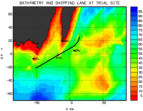
Figure 1. Bathymetry (meters) at the experimental site, with the hydrophone position marked as HYD. The shipping lane is indicated by the trajectory of the closest passage on October 2, 2014. The black dots marked UTL, SOU, GRU show the positions of the lighthouses Utlängan, Ölands Södra Udde, and Ölands Södra Grund, respectively.

FIGURE 2

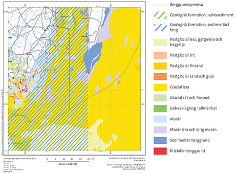
Figure 2. Sediment types at the experimental site [(The Geological Survey of Sweden (SGU), 2016)].

3. Transmission Loss Trial

In order to determine geoacoustical parameters capturing the sound propagation effects at the experimental site, a transmission loss measurement was performed. A loudspeaker emitting 30 s continuous wave pulses at 100, 150, 250, 350, 450, and 550 Hz was towed at distances 90–2,215 m from the bottom-mounted hydrophone (Figure 3). The signal from a hydrophone hanging from the towing boat together with data from the bottom-mounted hydrophone were then used to determine the transmission loss between the two hydrophones as

$\begin{array}{cc}TL=10{\text{ log}}_{10}\left(\frac{p_1^2}{p_2^2}\right)& \left(1\right)\end{array}$

where p₁ and p₂ is the pressure at the towed and the bottom mounted hydrophone, respectively. The bottom mounted Wildlife SM2M measurement system was calibrated in a standing wave tube resulting in sensitivity curves shown in Figure 4. For frequencies below 100 Hz and above 800 Hz, a constant extrapolation of the sensitivity is assumed. It should be noted that previous measurements using this equipment have indicated that below 100 Hz, the sensitivity may in fact be much lower, and hence the low frequency results should be taken with some caution, as discussed in Section 5.

FIGURE 3

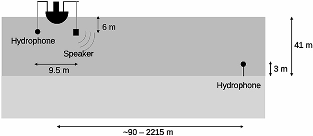
Figure 3. Experimental setup of the transmission loss trial dedicated to geoacoustical inversion.

FIGURE 4

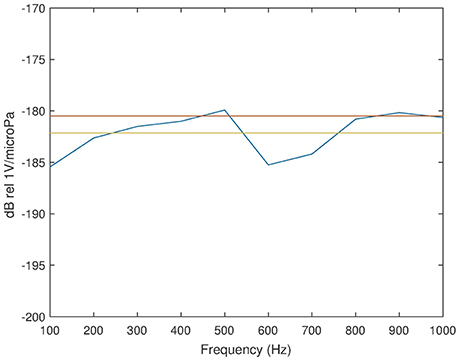
Figure 4. Sensitivity of the receiver chain as function of frequency: Calibrated in standing wave tube (blue), frequency average (yellow), and factory value (red).

The parameters of a range-independent seabed composed of a sediment layer above a bedrock halfspace were estimated from the observed TL data by geo-acoustic inversion using the differential evolution method (Snellen and Simmons, 2008), with the XFEM code (Karasalo, 1994) for range-independent layered media as forward model. The assumption of range-independence is motivated by the weak bathymetry variations observed in Figure 6, where the depth ranges from 41.6 to 43.9 m in a 2.5 × 2.5 km square centered at the hydrophone. The bounds of the parameter search regions and the obtained estimates are listed in columns 2–4 of Table 1. The choice of the search regions was guided by the map of sediment types shown in Figure 2 combined with data on typical acoustic parameters for sediment and rock materials (Ainslie, 2010, Table 4.18), (Bourbié et al., 1987, Table 5.2).

TABLE 1

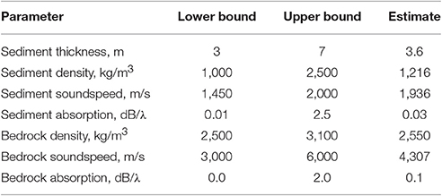
Table 1. Parameters of two-layer seabed model.

It should be noted that the purpose of the inversion is to find a simplified seabed model for which the predicted transmission losses are good approximations to the experimentally observed. The seabed model is then useful for reliable modeling of the bottom interactions at transmission loss prediction, however its parameters and structure do not necessarily correspond to those of the actual physical seabed. This argument is illustrated by Table 2 and Figure 5 below. Column 4 of Table 2 shows the seabed parameters obtained by acoustic inversion but with a different initialization of the random number generator used by the differential evolution algorithm. Both the sediment thickness and the material parameters of the individual layers are seen to be significantly different from those in column 4 of Table 1.

TABLE 2

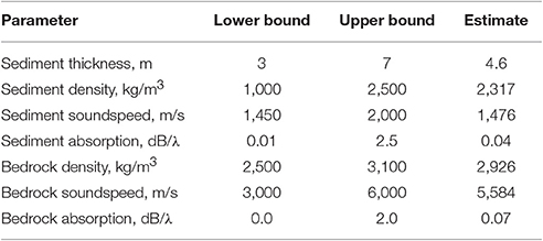
Table 2. Parameters of alternative two-layer seabed model.

FIGURE 5

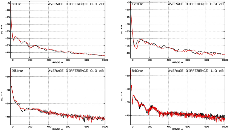
Figure 5. TL to the hydrophone as function of source range using sound speed data of 2014-10-18 combined with seabed parameters in, respectively, Table 1 (black) and Table 2 (red). Source depth 5 m.

Figure 5 compares the transmission losses TL₁(r) and TL₂(r) as function of source range r in the 63, 127, 254, and 640 Hz 1/3 octave bands, using soundspeed data for 2014-10-18 combined with the seabed parameters in, respectively, Table 1 [TL₁(r), black] and Table 2 [TL₂(r), red]. The source depth is 5 m.

The differences |TL₁(r) − TL₂(r)|, averaged over range r, are shown in the upper right hand corners of the four frames. The average differences of ≈1 dB or less indicate the uncertainty induced by unknown seabed parameters on the transmission losses used for source level estimation in Section 4 below. Similar results, not shown here, were obtained for a selection of dates in October–December 2014.

4. Estimation of the Source Levels

Estimates of the noise source spectra were computed for all ship passages of the hydrophone at range 1,000 m or less in the trial period October 2–December 29. The numbers of such passages and individual ships were 2,088 and 943, respectively. The noise source level was estimated in 21 1/3-octave bands with center frequencies $f_k=10\times 2^{(k-1)/3}\text{ Hz},$ ranging from f₁ = 10 Hz to f₂₁ = 1016 Hz.

The estimate SL_k of the noise source level (dB) in frequency band k was obtained as

$\begin{array}{cc}S{L}_k=R{L}_k+T{L}_k.& \left(2\right)\end{array}$

RL_k and TL_k are, respectively, estimates (dB) of the noise level at the hydrophone and the transmission loss from the source to the hydrophone when the ship is at its closest point of approach (CPA), i.e., when the range from the ship to the hydrophone is minimal. The computation of these estimates is described in Sections 4.1 and 4.2 below.

4.1. Estimation of the Noise Level at the Hydrophone

Let r_hyd denote the position of the hydrophone, r(t) the position of the ship as function of time t, and R(t) the range from the ship to the hydrophone

$\begin{array}{cc}R(t)=|r(t)-r_{\text{hyd}}|.& \left(3\right)\end{array}$

The function r(t) was defined as the piece-wise linear interpolant to AIS position data. Denote the minimum of R(t) by R_cpa = R(t_cpa).

Then the estimates of the noise levels N_k, (k = 1, …, 21) at the hydrophone excited by the ship from its CPA were computed as follows:

1. A time-interval with length T_tot = 240 s was selected, centered at t_cpa, and subdivided into M = 60 consequtive subintervals T_j, (j = 1, …, M) with equal lengths T_tot/M = 4 s.

2. Denote by s_j(t) the signal received by the hydrophone in subinterval T_j, j = 1, …, M and by

$\begin{array}{cc}{W}_j={\displaystyle {\int }_{T_j}{s}_j}{(t)}^{2}dt& \left(4\right)\end{array}$

the energy of s_j(t).

3. The subinterval j_cpa for which W_j is maximal was found and the short-time Fourier spectra ŝ_jcpa(f) of s_jcpa(t) were computed by FFT. Then the noise levels RL_k at the hydrophone excited by the ship from its CPA were estimated by

$\begin{array}{cc}R{L}_k=10{\text{ log}}_{10}\left\{{\displaystyle {\int }_{f_k^{-}}^{f_k^{+}}|{\widehat{s}}_{j_{\text{cpa}}}(}f){|}^{2}df\right\}k=1,...,21& \left(5\right)\end{array}$

where $f_k^{-}=2^{-1/6}{f}_k$ and $f_k^{+}=2^{1/6}{f}_k$ are the bounds of the 1/3-octave band with center frequency $f_k=10\times 2^{(k-1)/3}$ Hz.

To summarize, the received signal segment corresponding to sound emitted from the CPA of the ship was identified as the 4 s time-window in which the received sound energy (4) is maximal. The simpler alternative of using the timepoint t_cpa explicitly proved to be unreliable due to inaccurate time-synchronization between the AIS and the hydrophone data. Note that Equation (2) with RL_k defined by Equation (5) holds only when the received noise is dominated by that from the ship, a condition which was reasonably well-satisfied for ship passages within the selected maximal range of 1 km.

4.2. Estimation of Transmission Loss

The transmission losses TL_k, (k = 1, …, 21) from the CPA to the receiver hydrophone were estimated by sound propagation modeling. The following simplifying assumptions on the underwater medium were used:

1. The geometry and the medium parameters are range-independent, with water-depth equal to that at the hydrophone.

2. Variations of the sound speed profile within 1 day are negligible.

Assumption 1 was considered reasonable since (i) The variations of the water depth are only ca 2 m within the maximal range (1 km) to the CPAs used for the estimates as shown in Figure 6 and (ii) Data on the sound speed profile were available at a single spatial location only. Similarly, assumption 2 was found reasonable by inspection of the sound speed profile data. Figure 7 shows the sound speed profile at the measurement site every 6 h throughout the measurement period.

FIGURE 6

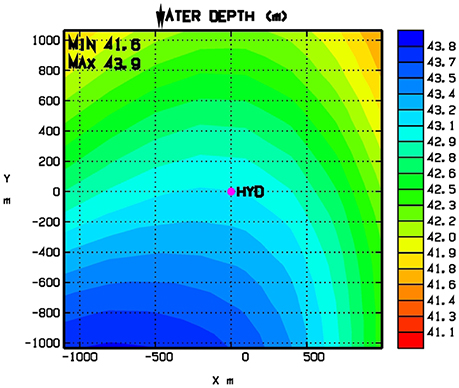
Figure 6. Water depth (meters) in a 2.5 × 2.5 km area centered at the hydrophone marked as HYD.

FIGURE 7

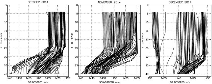
Figure 7. Sound speed profiles at the measurement site at 6 h intervals in October–December 2014, by the HIROMB oceanographic model (SMHI, 2016).

Under these assumptions the soundfield was computed with a full-field method for range-independent layered media (Ivansson and Karasalo, 1992; Karasalo, 1994; Karasalo and deWinter, 2006), based on adaptive high-order wavenumber integration and solution of the depth-separated wave equation by exact finite elements. The method is accurate at all ranges to the CPA, including in particular CPAs in the immediate nearfield of the hydrophone. Further, the modeled transmission loss is independent of the direction to the CPA, so that the estimates of the TLs from all CPAs on a given day and a given frequency were obtained by a single run of the propagation model to obtain the TL on a dense range grid followed by computation of the TLs from the individual CPAs by interpolation in range.

The transmission loss TL_k in 1/3 octave band nr k was estimated by

$\begin{array}{cc}T{L}_k=10{\text{ log}}_{10}\left\{\frac{1}{N}{\displaystyle \sum _{j=1}^{N}1}{0}^{TL(f_j)/10}\right\}k=1,...,21& \left(6\right)\end{array}$

where N = 7, TL(f) is the TL (dB) at frequency f and f_j are frequencies covering 1/3 octave band nr k with logf_j, (j = 1, …, N) equidistant.

5. Results

In Table 3, the number passages based on ship category is shown, together with statistics on speed, length, and displacement. Estimated median source spectra for the four categories with the most ship passages are given in Figure 9. One cargo ship was excluded because of incomplete data. For each ship passage, predictions of the source levels using four models are given:

1. The Wittekind model (Wittekind, 2014), requiring seven input parameters: cruise speed, displacement, cavitation inception speed, block coefficient, engine mass, number of engines in use, and an engine mount parameter.

2. The AQUO model (Audoly and Rizzuto, 2015), estimating the source levels based on ship category, cruise speed, and ship length.

3. The Wales-Heitmayer (WH) model (Wales and Heitmayer, 2002), providing an estimate based on statistics obtained from measurements on 272 ships. The WH model is independent of ship parameters, and hence gives a baseline spectrum which is identical for all ships.

4. The SONIC model (Brooker and Humphrey, 2015), giving a correction to the WH model based on cruise speed and a ship category specific reference speed. This model is not applicable to Tug.

TABLE 3

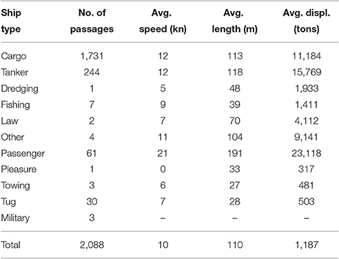
Table 3. Number of passages and average speed, length, and displacement per ship category.

Input parameters for the AQUO and the Wittekind models were obtained from AIS and the STEAM database. For more details, the reader is referred to the Appendix (Supplementary Material).

The accuracy of the source level predictions varies; for three of the ship categories, Cargo, Tanker, and Tug, the medians agree with the experimental data within 10 dB for frequencies above 200 Hz. For Cargo and Tanker, the AQUO model gives slightly better agreement with measurement data than Wittekind for most frequency bands. The Wittekind model clearly overestimates the source level for Passenger ferries. Meanwhile, the WH baseline spectrum agrees fairly well for this category. For frequencies below 200 Hz, the model-measurement agreements are generally poorer. Two possible causes for this are (i) deterioration of the calibration of the hydrophone at low frequencies and (ii) degradation of the signal to noise ratio caused by decrease of the transfer function amplitude with decreasing frequency. The second of these effects is investigated in Figure 8 showing the transmission loss on 2014-11-15 as function of frequency from a ship at range 200 m to the hydrophone. By the figure the cutoff frequency of the shallow-water medium is ~9 Hz. Thus the center frequencies of all the considered 1/3-octave bands are above cutoff, hence the model-measurement discrepancies at low frequencies are more likely caused by poor hydrophone calibration than by low S/N.

FIGURE 8

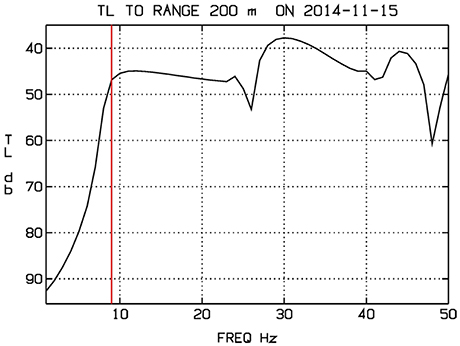
Figure 8. Model-predicted TL to the hydrophone from a ship at range 200 m, using sound speed data of 2014-11-15. The red line at indicates the cutoff frequency of the shallow-water medium.

Furthermore, Scrimger and Heitmeyer (1991) noted when comparing the source spectra from passenger ships, cargo ships, and tankers, that the differences between these were not significant. Similar observations can be made here by noting that the median levels of the experimental data for the these categories differ by no more than around 7 dB. This is to be compared to the ~20 dB predicted by the AQUO model and the Wittekind models' ~13 dB.

The source strengths are estimated from the experimental data assuming two different source depths, 2.5 and 5 m, to investigate the effect of this model parameter on the transmission loss. While the assumed source depth is not included explicitly in the source strength models, it is seen in Figure 9 to influence the predicted source strength by up to ~5 dB.

FIGURE 9

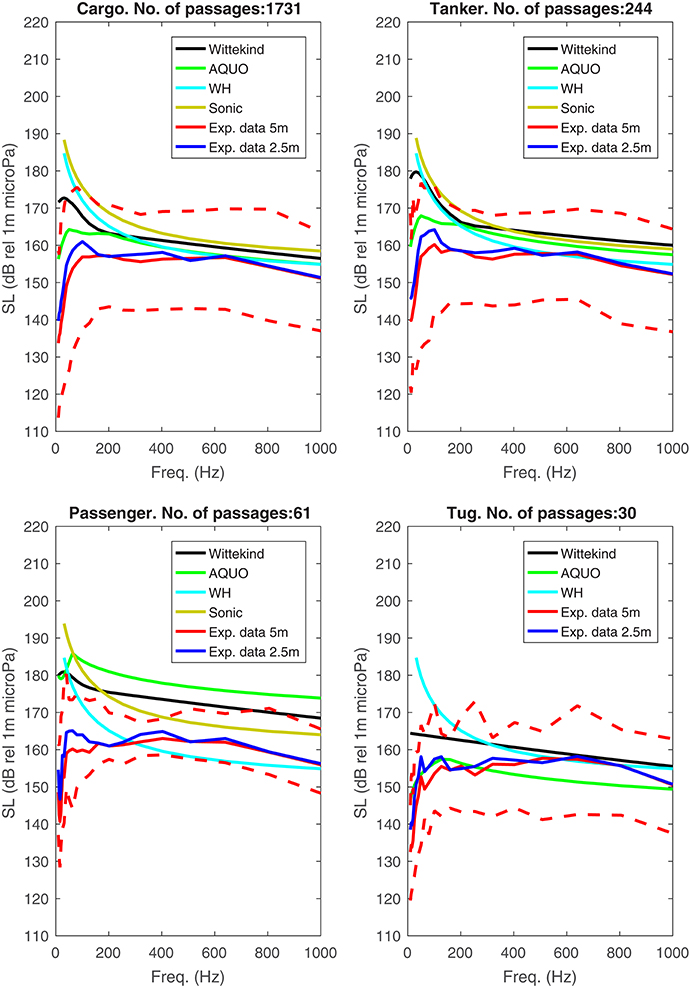
Figure 9. Source level spectra per category. Solid lines: Median, dashed lines: 99th and 1st percentile of 5 m depth measurement data.

Statistical variability measures in terms of the difference between the 99th and 1st percentile are shown in Figure 10. For Cargo and Tanker the variability of the measured source strengths is in the range of 20–30 dB above ~200 Hz while increasing to >40 dB at around 100 Hz, agreeing with what is observed by Simard et al. (2016). The observed Passenger ships notably show a smaller variability, not exceeding 20 dB for frequencies >200 Hz.

FIGURE 10

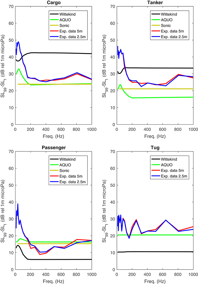
Figure 10. Difference between 99th and 1st percentile per category.

In Figures 11, 12 the source level estimates from two individual ships (the Ro-Ro Passenger ship Finnlady and the Ro-Ro Cargo ship Finnsky) passing near the hydrophone on 21 and 16 separate occasions, respectively, are depicted. For Finnlady, the median values of the Wittekind model matches the experimental data poorly, as previously observed for passenger ships. Moreover, the predicted variations are rather large, showing that the noise radiated from a single ship can vary as much as 20 dB. For the Finnsky ship, the variations are substantially smaller (~10 dB) and of the same magnitude as predicted by the AQUO and Sonic models. In Figures 13, 14 frequency averaged source levels, $\sum _{k=1}^{21}S{L}_k/21$, are plotted for each ship passage along with data on ship speed, hydrophone-CPA distance and wind speed. For neither of the ships, a clear correlation between these parameters and source level is discernible. Hence, the cause of the large source level variations for the Finnlady ship is as of now unclear. For a more rigorous investigation of the observed variations, more detailed data on the actual operating conditions for each ship passage would be needed, including e.g., data on engine power input, propeller cavitation and load carried by the ship.

FIGURE 11

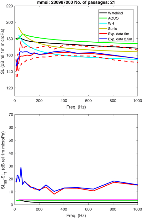
Figure 11. Top: Source level spectra of the Passenger/Ro-Ro Cargo ship Finnlady (IMO 9336268, MMSI 230987000) estimated from 21 close passages. Solid lines: Median, dashed lines: 99th and 1st percentile. Bottom: Difference between 99th and 1st percentile.

FIGURE 12

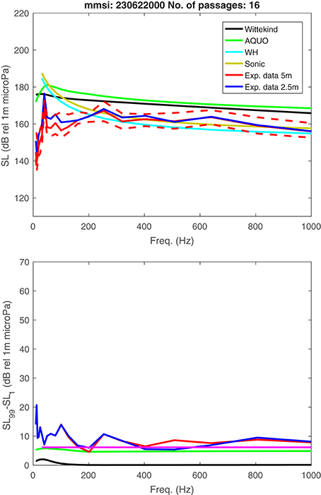
Figure 12. Top: Source level spectra of the Passenger/Ro-Ro Cargo ship Finnsky (IMO 9468906, MMSI 230622000) estimated from 21 close passages. Solid lines: Median, dashed lines: 99th and 1st percentile. Bottom: Difference between 99th and 1st percentile.

FIGURE 13

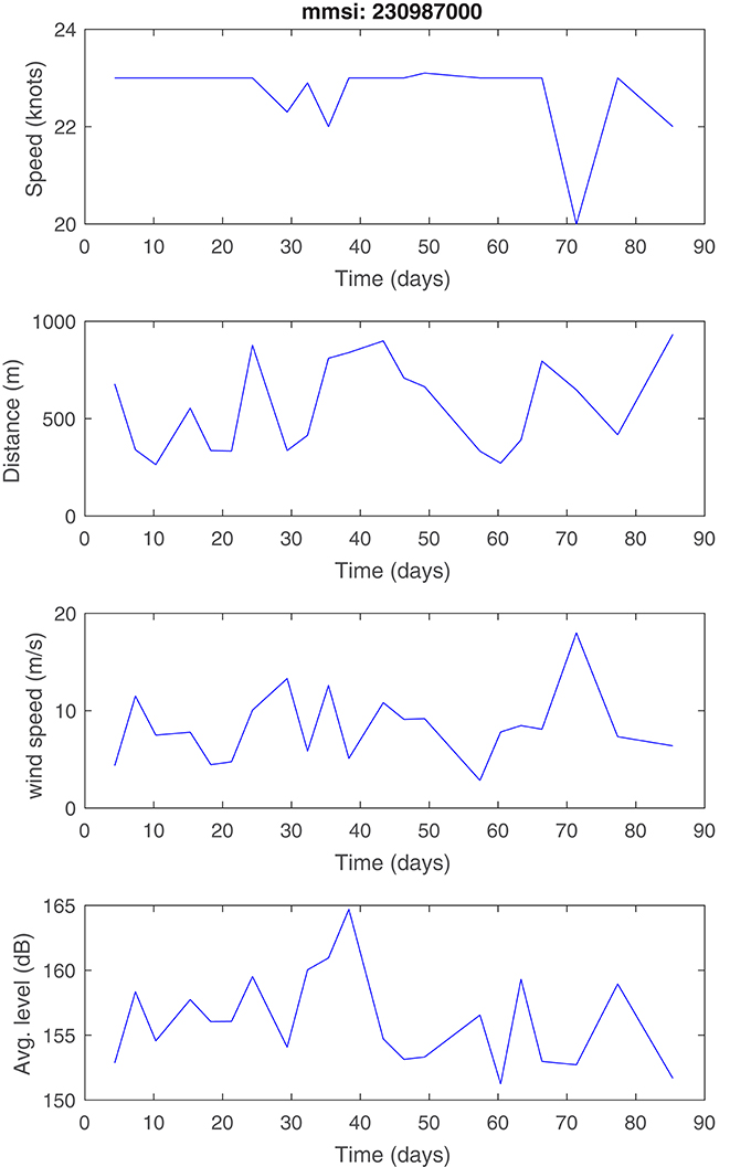
Figure 13. Source level averaged over frequency for each passage of the Passenger/Ro-Ro Cargo ship Finnlady (IMO 9336268, MMSI 230987000) along with data on ship speed, hydrophone-CPA distance and wind speed. Day zero is taken as October 1, 2014.

FIGURE 14

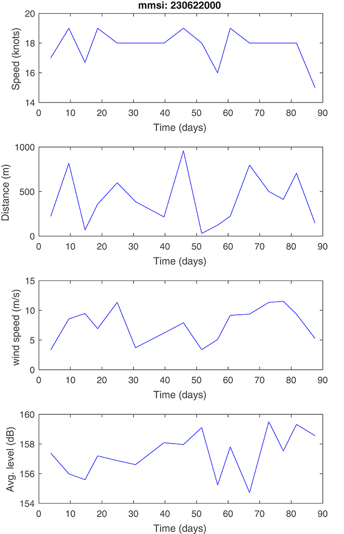
Figure 14. Source level averaged over frequency for each passage of the Passenger/Ro-Ro Cargo ship Finnsky (IMO 9468906, MMSI 230622000) along with data on ship speed, hydrophone-CPA distance and wind speed. Day zero is taken as October 1, 2014.

6. Summary and Conclusions

A procedure was presented for estimating the underwater radiated noise (URN) source spectra of individual ships using (i) sound recordings by a single hydrophone positioned near a major shipping lane in the Baltic Sea, (ii) AIS data on ship traffic in the area and (iii) sound propagation modeling to estimate the transmission loss from the closest point of approach of the ships to the hydrophone. Acoustic seabed parameters were estimated by geo-acoustic inversion of data from a transmission loss trial and sound speed profiles were obtained from the HIROMB oceanographic model.

The procedure was applied to estimate the source strength of over 900 individual ships from more than 2,000 close passages of the hydrophone during a 3 month period in 2014. Comparisons to source strength models found in the literature show, that for Tankers and Cargo ships, which are the most common ships in the Baltic Sea, these can provide reasonably good estimates of the median source levels above ~200 Hz. For the two other categories and for multiple passages by the same ship, larger discrepancies are present. The poor model-prediction agreement observed for low frequencies is likely due to the lack of reliable hydrophone calibration data. In future studies, it is desirable to extend the lower frequency limit of the methodology in order to cover the lowest indicator frequency (63 Hz) of the Marine Strategy Framework Directive adopted by the European Union.

The estimation procedure and the collected data can, in light of the discrepancies observed, be used to enhance the reliability of existing source strength models. Considering that the awareness of the adverse effects of URN on underwater fauna is increasing, such models along with statistics as presented here can be used to more accurately direct URN mitigation efforts.

Author Contributions

IK and MÖ provided estimates of the seabed parameters by acoustic inversion of the transmission loss trial data and of the source spectra from the long-term recordings. PS carried out the transmission loss trial. JJ and LJ provided the Wittekind noise source results based on FMI STEAM model, and participated together with ML and RB in manuscript writing and result analysis.

Funding

Funding for this work was received from the EU through SHEBA (Sustainable shipping and environment of the Baltic sea region), a BONUS (Baltic Organisations' Network for Funding Science) research project, call 2014-41 (www.bonusportal.org/projects/research_projects/sheba).

Conflict of Interest Statement

The authors declare that the research was conducted in the absence of any commercial or financial relationships that could be construed as a potential conflict of interest.

References

Ainslie, M. (2010). Principles of Sonar Performance Modelling. Berlin; Heidelberg: Springer-Verlag.

Google Scholar

ANSI (2009). ANSI/ASA S12-64: Quantities and Procedures for Description and Measurement of Underwater Sound From Ships – Part 1: General Requirements. New York, NY: Acoustical Society of America.

Arveson, P. T., and Vendittis, D. J. (2000). Radiated noise characteristics of a modern cargo ship. J. Acoust. Soc. Am. 107, 118–129. doi: 10.1121/1.428344

PubMed Abstract | CrossRef Full Text | Google Scholar

Audoly, C., and Rizzuto, E. (2015). Ship Underwater Radiated Noise Patterns. Technical report, AQUO - Achieve QUieter Oceans by shipping noise footprint reduction, FP7 - Collaborative Project no 314227, Deliverable R2.9.

Baltic Sea Hydrographic Commission (2016). Baltic Sea Bathymetry Database. Available online at: http://www.bsch.pro

Bourbié, T., Coussy, O., and Zinszner, B. (1987). Acoustics of Porous Media. Houston, TX: Gulf Publishing Company.

Google Scholar

Breeding, J. E., Pflug, L. A., Bradley, E. L., Walrod, M. H., and McBride, W. (1996). Research Ambient Noise Directionality (randi) 3.1 - Physics Description. Technical report, Technical Report NRL/FR/7176-95-9628, Naval Research Laboratory.

Brooker, A. G., and Humphrey, V. F. (2015). Noise Model for Radiated Noise/Source Level (Intermediate). Technical report, SONIC, Suppression Of underwater Noise Induced by Cavitation, FP7-314394-SONIC, Deliverable 2.3.

De Robertis, A., Wilson, C. D., Furnish, S. R., and Dahl, P. H. (2013). Underwater radiated noise measurements of a noise-reduced fisheries research vessel. ICES J. Mar. Sci. 70, 480–484. doi: 10.1093/icesjms/fss172

CrossRef Full Text | Google Scholar

Hatch, L., Clark, C., Merrick, R., Parijs, S. V., Ponirakis, D., Schwehr, K., et al. (2008). Characterizing the relative contributions of large vessels to total ocean noise fields: a case study using the gerry e. studds stellwagen bank national marine sanctuary. Environ. Manag. 42, 735–752. doi: 10.1007/s00267-008-9169-4

PubMed Abstract | CrossRef Full Text | Google Scholar

Ivansson, S., and Karasalo, I. (1992). A high-order adaptive integration method for wave propagation in range-independent fluid-solid media. J. Acoust. Soc. Am. 92, 1569–1577.

Google Scholar

Jalkanen, J.-P., Johansson, L., Kukkonen, J., Brink, A., Kalli, J., and Stipa, T. (2012). Extension of an assessment model of ship traffic exhaust emissions for particulate matter and carbon monoxide. Atmos. Chem. Phys. 12, 2641–2659. doi: 10.5194/acp-12-2641-2012

CrossRef Full Text | Google Scholar

Karasalo, I. (1994). Exact finite elements for wave propagation in range-independent fluid-solid media. J. Sound Vib. 172, 671–688.

Google Scholar

Karasalo, I., and deWinter, J. (2006). “Airy function elements for inhomogeneous fluid layers,” in Proceedings of the 8th European Conference on Underwater Acoustics, eds S. M. Jesus and O. C. Rodriguez (Carvoeiro: University of Algarve), 33–38.

NEXUS MEDIA (2005). Marine Engines – A Motorship Supplement, 2005 Guide, a Comprehensive a-z Listing of Marine Diesel Engines in Excess of 300 kw. Technical report.

Rolland, R. M., Parks, S. E., Hunt, K. E., Castellote, M., Corkeron, P. J., Nowacek, D. P., et al. (2012). Evidence that ship noise increases stress in right whales. Proc. R. Soc. Lond. B Biol. Sci. 279, 2363–2368. doi: 10.1098/rspb.2011.2429

PubMed Abstract | CrossRef Full Text | Google Scholar

Rowen, A. L. (2003). Ship Design and Construction, Volume 1, Chapter 24: Machinery Considerations. The Society of Naval Architects and Marine Engineers (SNAME).

Scrimger, P., and Heitmeyer, R. M. (1991). Acoustic source-level measurements for a variety of merchant ships. J. Acoust. Soc. Am. 89, 691–699.

Google Scholar

Simard, Y., Roy, N., Gervaise, C., and Giard, S. (2016). Analysis and modeling of 255 source levels of merchant ships from an acoustic observatory along St. Lawrence seaway. J. Acoust. Soc. Am. 140, 2002–2018. doi: 10.1121/1.4962557

PubMed Abstract | CrossRef Full Text | Google Scholar

SMHI (2016). High Resolution Operational Model for the Baltic Sea. Available online at: http://www.smhi.se/forskning/forskningsomraden/oceanografi/hiromb-1.543

Snellen, M., and Simmons, D. (2008). An assessment of the performance of global optimization methods for geo-acoustic inversion. J. Comput. Acoust. 16, 199–223. doi: 10.1142/S0218396X08003579

CrossRef Full Text | Google Scholar

The Geological Survey of Sweden (SGU) (2016). Available online at: http://www.sgu.se

Wales, S. C., and Heitmayer, R. M. (2002). An ensemble source spectra model for merchant ship-radiated noise. J. Acoust. Soc. Am. 111, 1211–1231. doi: 10.1121/1.1427355

PubMed Abstract | CrossRef Full Text | Google Scholar

Watson, D. G. M. (1998). Practical Ship Design. Oxford: Elsevier Science.

Google Scholar

Wittekind, D. K. (2014). A simple model for the underwater noise source level of ships. J. Ship Prod. Design 30, 1–8. doi: 10.5957/JSPD.30.1.120052

CrossRef Full Text | Google Scholar

Appendix

Acquisition of Ship Parameters

For the Wittekind noise source model, several parameters are required which are not part of commercially available databases of ship specifications. The engine mass data were obtained from the Marine Engines catalog (NEXUS MEDIA, 2005) and augmented with data from engine manufacturers. Based on these data, linear relationships between engine power and engine mass was determined and used for cases where no data could be obtained from other sources. How to determine the number of operating engines and Block coefficient (C_b) is described by Jalkanen et al. (2012), where power prediction formulas are employed to determine the number of operating engines. Hull form parameters were estimated according to Watson (1998). Engine mounting parameter for resiliently and rigidly mounted engines were assigned according to Rowen (2003). Cavitation inception speed was estimated in terms of block coefficient and vessel design speed, V_d, as

$\begin{array}{cc}{V}_{\text{CIS}}=\min \{\max [(1.42-1.2C_{\text{b}})V_{\text{d}},9],14\}.& \left(\text{A}1\right)\end{array}$

Cavitation inception speed can significantly affect the predicted noise source levels, but this parameter is very difficult to predict based on available information of the propulsors of the world fleet. Undoubtedly, prediction of V_CIS using expression (A1) may introduce a significant source of uncertainty to noise source modeling and further work is needed to describe cavitation inception speed as accurately as possible.