A Comparison between Four Analytical Methods for the Measurement of Fe(II) at Nanomolar Concentrations in Coastal Seawater

Introduction

Standardization of trace metal clean sampling techniques, inter-comparison exercises and the widespread use of consensus seawater reference samples have led to reproducible measurements of dissolved (<0.20 μm) Fe concentrations in full depth profiles of all major ocean basins (Mawji et al., 2015), vastly improving our understanding of Fe biogeochemistry in the ocean. Such extensive exercises, however, have not yet been widely conducted with transient species such as Fe(II) which, due to their short-lived and highly reactive nature, present many challenges to the analyst. The rapid oxidation rate of Fe(II) in oxic seawater (King et al., 1995; Santana-Casiano et al., 2005; Sarthou et al., 2011), and the sensitivity of Fe(II) concentration and oxidation/reduction rates to multiple variables including pH, temperature, light intensity, dissolved oxygen (O₂), reactive oxygen species (ROS) and natural organic material (NOM; Davison and Seed, 1983; Millero et al., 1987; Rose and Waite, 2002) make sample collection logistically challenging and mean that the accuracy of Fe(II) measurements is difficult to verify.

Fe redox chemistry is an important feature of the marine Fe cycle. In surface waters, photochemical processes form dissolved Fe(II) from Fe(III) either directly by photoreduction of Fe(III) species, or indirectly via ROS (O'Sullivan et al., 1991; Barbeau, 2006; Croot et al., 2008). Dissolved Fe(II), whilst short-lived in oxic seawater, accounts for a large fraction of dissolved Fe (DFe) entering the ocean from shelf sediments in oxygen minimum zones (OMZs; Lohan and Bruland, 2008; Vedamati et al., 2014), from hydrothermal vents (Statham et al., 2005; Sedwick et al., 2015), from rainwater (Zhuang et al., 1995; Willey et al., 2008) and possibly also from ice melt (Lin and Twining, 2012). From an energetic perspective, Fe(II) is expected to be more bioavailable than Fe(III) (Sunda et al., 2001). Furthermore, regardless of whether dissolved Fe(II) is actually more bioavailable than dissolved Fe(III) to specific cellular uptake systems, redox cycling in oxic waters is always expected to have the net effect of maintaining Fe in more labile phases (Croot et al., 2001; Emmenegger et al., 2001) due to the enhanced solubility of Fe(II) relative to Fe(III).

The impracticality of creating stable transient-species reference materials, means that uncertainties remain about how comparable and how accurate existing Fe(II) data are. This is especially the case at nanomolar Fe(II) concentrations (which can occur, for example, in coastal waters, estuaries and OMZs) where multiple methods are available, each with different potential interferences and analytical constraints. In broad terms three different analytical approaches have been taken to measure Fe(II) concentrations in natural waters: luminol based chemiluminescence (Seitz and Hercules, 1972; O'Sullivan et al., 1995; Bowie et al., 2002), spectrophotometric methods using ferrozine (Stookey, 1970; Waterbury et al., 1997) or other synthetic ligands (Smith et al., 1952; Hennessy et al., 1984), and voltammetry (Gledhill and Van Den Berg, 1995). Luminol based flow injection techniques are by far the most commonly used to measure Fe(II) concentrations at sea, largely because of the sub-nanomolar detection limit that can be achieved (Bowie et al., 2002; Hansard and Landing, 2009), but other methods are still actively used in several different environments and applications. Ferrozine, for example, remains the most common analytical approach used in both autonomous Fe(II) sensors (Chin et al., 1994; Sarradin et al., 2005) and also in freshwater and estuarine environments (Kieber et al., 2001; Statham et al., 2012).

Here, we compare four analytical methods for the determination of nanomolar Fe(II) concentrations in coastal seawater. We aim to assess the uncertainty associated with measuring and interpreting Fe(II) concentrations in natural waters via different analytical approaches. The four approaches selected for comparison were: ferrozine (Waterbury et al., 1997), Cathodic Stripping Voltammetry (CSV; Gledhill and Van Den Berg, 1995), and flow injection analysis (FIA) using luminol chemiluminescence both with (Bowie et al., 2002) and without (Croot and Laan, 2002) a pre-concentration step. In this study, in order to assess whether Fe(II) methods produce comparable Fe(II) concentrations and oxidation rates under environmentally relevant conditions, the experimental conditions for a series of method comparison experiments were selected to test the hypothesis that Fe(II) stability in coastal seawater is substantially affected by small changes in NOM composition and initial Fe(II) concentration. Varying spikes of Fe(II) were added to batches of Mediterranean seawater under pre-bloom conditions, post-bloom conditions (after a mesocosm experiment) and after addition of a humic/fulvic spike to represent high NOM estuarine waters.

Materials and Methods

A series of eight method comparison experiments (Table 1) were conducted in Crete (June 2016). Coastal seawater was collected using acid cleaned (0.3 M HCl soak for 3 days followed by 3 de-ionized water and 3 seawater rinses) tubing and high density polyethylene (HDPE) containers. Seawater was used either as collected or, in order to adjust the sample matrix with respect to NOM that may adversely affect Fe redox chemistry in coastal seawater (Santana-Casiano et al., 2000; Rose and Waite, 2003), under post-bloom conditions after a mesocosm experiment. The 12 day mesocosm was conducted as part of the Ocean Certain project in 1,500 L HDPE containers (cleaned as above) where macronutrients had been added daily [6 nM phosphate, 48 nM nitrate, 48 nM ammonium and silicic acid as necessary to maintain an excess according to the Redfield ratio (Redfield, 1934)] to stimulate a phytoplankton bloom. In both cases, seawater was stored under reduced lighting conditions for >3 days prior to the Fe(II) method comparison experiments, in order to lower the concentration of ROS.

TABLE 1

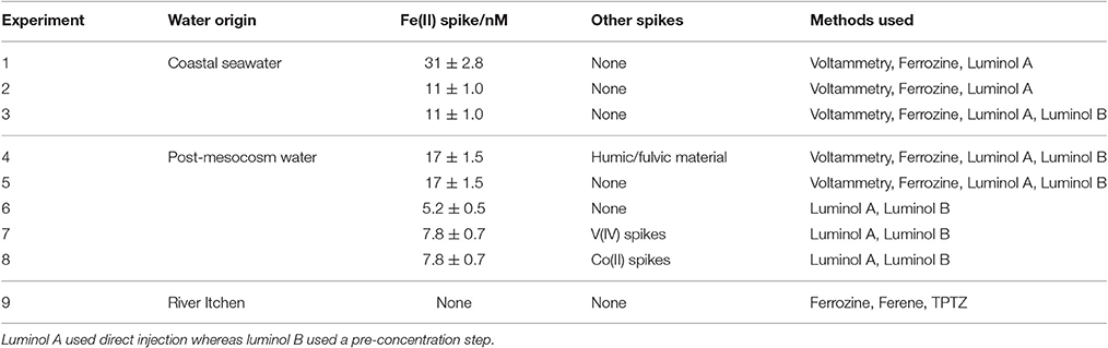
Table 1. Set up of nine method comparison experiments where Fe(II) concentrations were measured simultaneously using multiple methods.

In addition to the comparison of luminol (with, and without, pre-concentration), ferrozine and voltammetry methods for Fe(II) analysis in Mediterranean seawater, potential artifacts associated with spectrophotometric analysis of Fe(II) concentrations were investigated using three different commercially available synthetic Fe(II) ligands: ferrozine (as per the 4-method comparison in coastal seawater), ferene and 2,4,6-tripyridyl-2-triazine (TPTZ). As spectrophotometric methods are most commonly used in freshwater, this comparison was undertaken using aged River Itchen (Southampton, UK) water which was filtered (0.2 μm) into 1 L low density polyethylene (LDPE) bottles and then stored at 6°C in the dark. The River Itchen was selected for its relatively high pH (typically ~8) and modest DFe (100–500 nM) content (Statham et al., 2012; Hopwood et al., 2015).

Method Comparison Experiments in Spiked Seawater

Eight method comparison experiments were conducted in Mediterranean seawater using a combination of the selected methods to measure Fe(II) concentrations in either 20 or 2 L containers over time periods of 0.5–2 h after 5 to 31 nM spikes of dissolved Fe(II) were added (1–8, Table 1). Both 20 L and 2 L containers were pre-cleaned with mucasol detergent (Sigma-Aldrich) for 1 day, followed by 1 week in 1.2 M HCl with 3 de-ionized water rinses after each stage. Experiments were carried out in a temperature controlled room (measured range 19.9–21.5°C), where coastal seawater was stored prior to commencing experiments, to ensure a near constant seawater temperature. The two FIA instruments (A-no pre-concentration, B-with a pre-concentration column) were placed adjacent to the experiment container. Analysis using voltammetry and spectroscopy was undertaken in a nearby temporary trace metal clean room where all surfaces were covered with plastic sheeting, the air was continuously filtered through polyester dust filters and clean suits were worn by the analysts. Stock solutions, reagents, manipulated seawater solutions and sample vials were prepared and handled in laminar flow hoods within the temporary trace metal clean room.

An Fe(II) stock solution was prepared from ammonium Fe(II) sulfate hexahydrate (99.997% Sigma Aldrich) in de-ionized water acidified with 1 μL HCl (trace metal grade, Fisher) per mL solution. A 1 μM Fe(II) stock solution was made daily and diluted to make standard additions and spikes. Prior to commencing experiments, N₂ (99.999% purity) was gently bubbled through aged seawater for 3–12 h to lower the dissolved O₂concentration and thus reduce the anticipated oxidation rate of added Fe(II) spikes (Santana-Casiano et al., 2005). 20 L collapsible low density polyethylene (LDPE) containers, filled with coastal seawater, were subject to external pressure to minimize the air headspace and gas exchange during the experiments. Experiments comparing only the two luminol based methods (numbers 6–8, Table 1) were undertaken in 2 L opaque HDPE containers with a constant, gentle stream of N₂ gas bubbles throughout the experiment.

For all method comparison experiments, an Fe(II) spike was added at time zero and followed by immediate mixing (inversion of the containers by hand) for ~30 s. For one experiment (number 4, Table 1) a spike of 10 mL humic/fulvic stock solution (unfiltered) was added before the seawater was bubbled with N₂. The two luminol-based Fe(II) FIA methods had polytetrafluoroethylene (PTFE) sampling lines running straight into the experimental containers, i.e., no sub-sampling of discrete aliquots was required from either 20 or 2 L containers. For the voltammetry and ferrozine methods, sub-samples were collected using a plastic syringe through a sample line also fitted into the 20 L experimental container. The sample line was first rinsed using the experimental seawater. 50 mL aliquots of seawater were then collected and immediately emptied into trace metal clean, opaque 125 mL HDPE sample bottles which were pre-laced with reagents. The time at which these sub-samples were collected was recorded (specifically the time at which the 50 mL sample was emptied into the pre-prepared vials). Full details of apparatus and analytical procedures for the four Fe(II) methods is included in Supplementary Material.

As much standardization as possible was introduced across the four techniques for Fe(II) analysis in Mediterranean seawater. The same 1 μM Fe(II) stock solutions were used by all analysts, vials and reagent bottles were all pre-prepared according to the same cleaning procedure and, where chemicals were used by multiple methods, the same reagent supplies were used. For two reasons it was not considered necessary, or desirable, for analysts to be unaware of the spiked concentration of Fe(II). First, all methods had to be calibrated over the expected range of Fe(II) concentrations (something which could normally be estimated roughly based on ambient water conditions). Second, there was already considerable uncertainty concerning the starting dissolved O₂ concentration, and therefore also the Fe(II) concentration at the first measured time point (which was always >1 min after the Fe(II) spike was made at t = 0 due to the requirement for mixing). The dissolved O₂ concentration was only known after the completion of each method comparison experiment.

For each spiked method comparison experiment (1–8, Table 1) the calculated Fe(II) oxidation rate constant (assumed to be first order with respect to [Fe(II)]) was derived from Millero et al. (1987) using measured salinity, temperature, dissolved O₂, pH (Table 2) and the corresponding values for K_w and I. The expected Fe(II) oxidation rate was also estimated from Roy and Wells (2011) using the two surface (5 m depth) oxidation rate constants reported (at 25°C and pH 8.0) from Ocean Station Papa (North Pacific). These apparent rate constants were adjusted for dissolved O₂ as per equations 1 and 2 (originally assumed to be saturated, now presented for measured dissolved O₂ concentrations, Table 2); but not for the discrepancies in salinity, temperature or pH as these were small and the relationships with k not derived in the original dataset.

$\begin{array}{ll}-\frac{\text{d}\left[\text{Fe}(\text{II})\right]}{\text{dt}}={\text{k}}_1\left[\text{Fe}(\text{II})\right]& (1)\end{array}$

$\begin{array}{ll}-\frac{\text{d}\left[\text{Fe}(\text{II})\right]}{\text{dt}}=\text{ k}\left[\text{Fe}(\text{II})\right]\left[{\text{O}}_2\right]{\left[\text{O}{\text{H}}^{-}\right]}^2& (2)\end{array}$

Total dissolvable Fe (TdFe) samples (unfiltered) were collected at the last time point for each of the method comparison experiments 1–8 (Table 1) in trace metal clean 125 mL LDPE (Nalgene) bottles. TdFe samples were then acidified to pH <2.0 by the addition of HCl (150 μL, UPA grade, Romil) and stored upright for 6 months prior to analysis. Samples were then diluted using 1 M distilled HNO₃ (Spa grade, Romil, distilled using a sub-boiling PFA distillation system, DST-1000, Savillex), and subsequently analyzed by high resolution inductively coupled plasma-mass spectrometry (HR-ICP-MS, ELEMENT II XR, ThermoFisherScientific) with calibration by standard addition. H₂O₂ (unfiltered) samples were also collected at the last time point in opaque HDPE (Nalgene) bottles and analyzed by luminol chemiluminescence (Yuan and Shiller, 1999), ~2 h after collection (stored in the dark at 20°C) to allow time for Fe(II) to decay to background levels. Total organic carbon (TOC, unfiltered) samples were collected at the same time in pre-combusted 50 mL glass vials, preserved by the addition of 100 μL HCl (trace metal grade, Fisher) and subsequently analyzed by high-temperature combustion analysis (Farmer and Hansell, 2007) (Shimadzu TOC-L Total Organic Carbon Analyzer).

TABLE 2

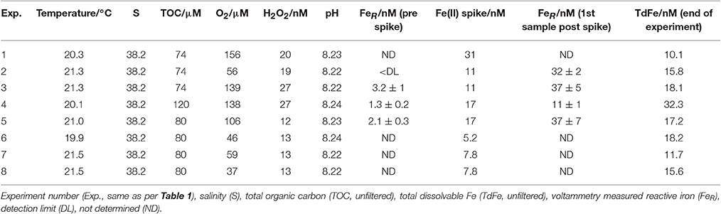
Table 2. Experimental conditions for a series of method comparison experiments where an Fe(II) spike was added to Mediterranean seawater and the concentration of Fe(II) then measured continuously until below detection.

For method comparison experiments 1–8 (Table 1), water samples for carbonate parameters and dissolved O₂ analysis were collected 5 min after commencing each experiment (approximately corresponding to the first voltammetry/ferrozine time point). Dissolved O₂ was measured using an Oxyminisensor (World Precision Instruments). Total alkalinity and dissolved inorganic carbon measurements were made on a VINDTA 3C system (Marianda, Kiel, Germany), then used to calculate pH (reported at the experimental temperature on the free pH scale) as per Tynan et al. (2016). Conversion of pH from carbonate parameters determined at 25°C, to pH_free values at the experimental temperatures was done using CO2SYS in MATLAB (van Heuven et al., 2011).

A humic/fulvic organic stock solution was prepared by adding 50 mg Suwannee River humic acid standard I and 50 mg Suwannee River fulvic acid standard II (International Humic Substances Society, IHSS, used as received) to 20 mL de-ionized water (Milli-Q,18.2 MΩ·cm) and then allowed to stand for 2 days at 6°C in the dark without filtration. Co(II) and V(IV) interferences, with luminol A and B, were tested by spiking Co(II) and V(IV) into the seawater matrix used for method comparison experiments 7 and 8 (Table 1) after Fe(II) concentration fell below the detection limit of both methods. Calculated spikes of 0.10 nM Co(II), 1.0 nM Co(II), 2.0 nM Co(II), 0.95 nM V(IV), 4.7 nM V(IV) and 47 nM V(IV) were added sequentially.

Method Comparison of Ferrozine, Ferene, and TPTZ in River Water

A comparison of different Fe(II) ligands used for spectrophotometric analysis was made using River Itchen (Southampton, UK) water (experiment 9, Table 1). The ligands ferene (3-(2-pyridyl)-5,6-bis(2-(5-furyl sulfonic acid))-1,2,4-triazine (Hennessy et al., 1984) and TPTZ (Collins and Diehl, 1960) were used to determine Fe(II) concentrations spectrophotometrically with the LWCC apparatus as described for ferrozine (Supplementary Material), but with the first monitored wavelength for peak absorbance changed from 562 to 593 nm. 10 mM stock solutions of ferene were made in de-ionized water, whereas 10 mM stock solutions of TPTZ were made in de-ionized water acidified to pH 3 by addition of HCl (trace metal grade, Fisher). Prior to analysis, filtered (0.2 μm) River Itchen water was stored in the dark at 6°C for 1 week. 500 μL ammonium acetate buffer (pH 8) was then added to 10 mL aged river water aliquots followed by a Fe(II) ligand (ferene/TPTZ/ferrozine) to a final ligand concentration of 40 μM. After a mixing time of between 2 min and 20 h in the dark at room temperature, the sample was loaded into a LWCC and absorbance measured. Further experiments were conducted with varying concentrations (40–1,000 μM) of ferrozine.

Results

Summary of Seawater Method Comparison Experiments

Measurement of TOC (74 μM in coastal seawater, 80 μM in post-mesocosm water), and pH (8.22 to 8.24) in the experimental seawaters verified that the composition was relatively homogeneous across the different water batches (Table 2). TOC determined on Deep Sea Water reference material (Batch 8–2008, Hansell Laboratory) was 45 ± 0.9 μM (consensus value 41–43 μM). After 3–7 days stored under reduced lighting conditions, H₂O₂ was significantly lower (12–27 nM) than the original concentration measured when the seawater was collected (90 nM for coastal seawater and 70 nM for post-mesocosm water). Combined with the applied deoxygenation, the reduced H₂O₂ concentrations should have slowed the oxidation rate of added Fe(II) spikes (Millero and Sotolongo, 1989). Dissolved O₂ (measured 5 min after commencing method comparison experiments 1–8) varied from 37–156 μM. Dissolved O₂ may have increased during experiments 1–5 (Table 1), which were conducted without a continuous flow of N₂. Whilst this may have increased the rate of Fe(II) oxidation with time, it should not have affected the comparison of methods.

Analysis of the Certified Reference Materials NASS-7 and CASS-6 via ICP-MS yielded Fe concentrations of 6.21 ± 0.62 nM (NASS-7, certified 6.29 ± 0.47) and 26.6 ± 0.71 nM (CASS-6, certified 27.9 ± 2.1). TdFe (collected at the end of experiments 1–8), was generally within the range expected for coastal seawaters (Table 2). For the experiments where large Fe(II) spikes were added (up to 31 nM), the added Fe(II) spike was no longer present in solution (as DFe), or in suspension (as TdFe), at the end of the experiments (~1 h after spike addition). This is consistent with the low solubility of Fe(III) in seawater (Millero et al., 1995; Millero, 1998) and the added Fe(II) spike adsorbing and/or precipitating on the container walls after oxidation. One exception was the humic/fulvic spiked experiment (Table 2), where 32 nM TdFe remained in suspension at the end of the experiment which most likely indicated the presence of more stable Fe(III)-organic complexes or colloids (Kuma et al., 1998) following Fe(II) oxidation. All the experiments used relatively high spikes of Fe(II) (5.2 to 31 nM) which was necessary to keep the Fe(II) concentration above the detection limit (Table 3) of all methods for multiple datapoints. Whilst not representative of open ocean or oxic shelf waters, where reported Fe(II) concentrations are typically picomolar (Ussher et al., 2007; Hansard et al., 2009; Sarthou et al., 2011), our experimental conditions (Table 2) form a reasonable representation of conditions within tropical OMZs where Fe(II) concentrations on the order of 10–100 nM can be found in coastal waters (Hong and Kester, 1986; Lohan and Bruland, 2008; Vedamati et al., 2014).

TABLE 3

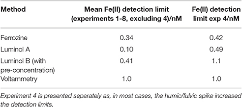
Table 3. Mean Fe(II) detection limits (defined as 3 standard deviations of an aged seawater blank for luminol A/voltammetry/ferrozine; and as 3 standard deviations of an analytical cycle without sample flow for luminol B) determined during the method comparison exercise.

Detection limits for Fe(II) were defined as 3 standard deviations of observed concentrations in seawater stored in the dark at 21°C (determined after the addition of all components to seawater other than the Fe(II) spike) for luminol A/voltammetry/ferrozine, and as 3 standard deviations of observed concentrations for an analytical cycle without sample flow for luminol B. In all cases detection limits were sufficiently low to measure the initial decline in Fe(II) concentration. Mean detection limits (Table 3) exclude experiment 4 where the addition of riverine NOM caused much higher detection limits for all methods except voltammetry.

Comparison of Fe(II) Results from Spiked Seawater Experiments

Luminol A

In all Fe(II) method comparison experiments in seawater (1–8, Table 1), the luminol A approach showed a decline in Fe(II) concentrations from 52 to 110% of the initial Fe(II) concentration added to below the detection limit of the method (Figure 1). The propagated uncertainty in the concentration of Fe(II) added to the seawater matrix at time zero ([Fe(II)]_t0) was ± 9%. The initial Fe(II) measurement, which for luminol A occurred 72–247 s after the spike addition, was always expected to be less than [Fe(II)]_t0. The most likely explanation for the slight overestimate of Fe(II) concentration (which was always <101% [Fe(II)]_t0, except for experiment 8) was the modest uncertainty associated with the initial spiked concentration.

FIGURE 1

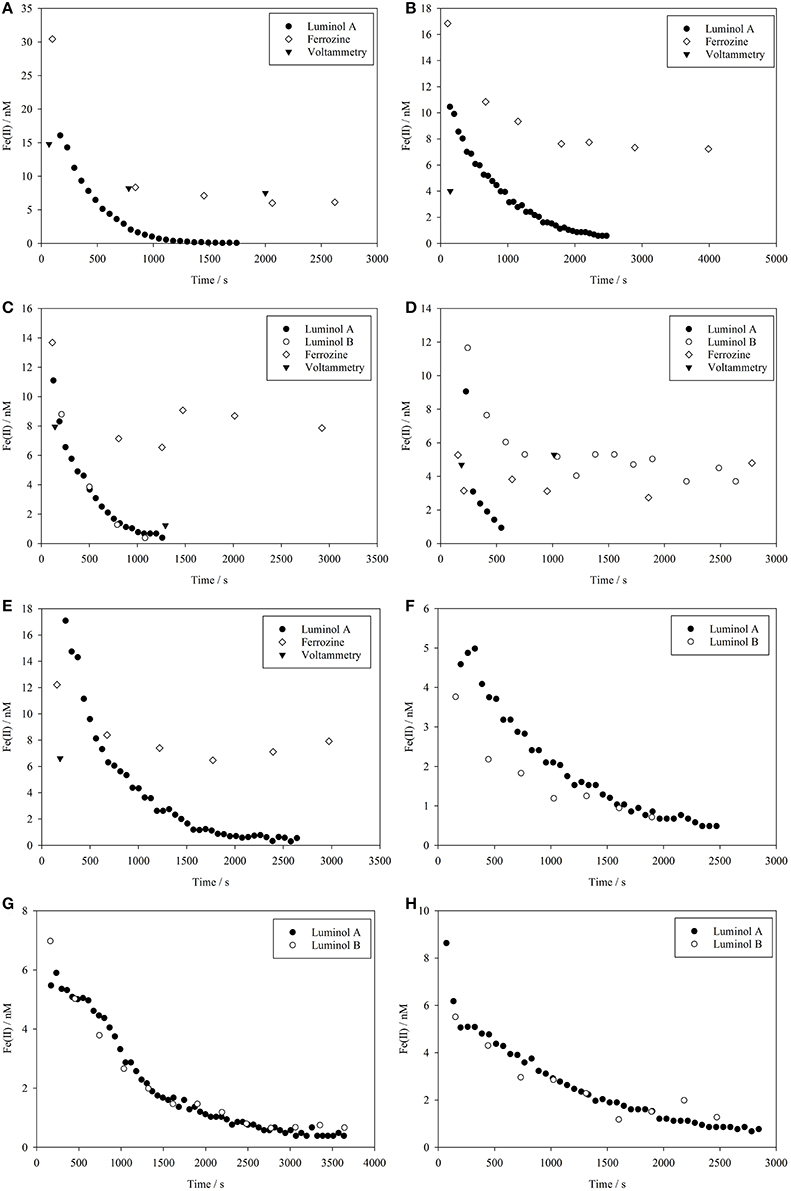
Figure 1. Fe(II) concentrations measured using multiple methods during a series of eight method comparison experiments where Fe(II) was spiked into coastal seawater at t = 0. (A–H) Correspond to experiments 1–8 as per Tables 1 and 2.

Luminol B

The luminol B approach produced data with a lower temporal resolution due to the longer analytical cycle required for pre-concentration (3.5 min compared to 1.0 min for luminol A) and was only used in experiments 3–8 (Table 1). As a result of a poor calibration for experiment 5, data for this experiment was flagged (the suspected reason was the incomplete removal of organic material on the 8-HQ column from the previous experiment). For the five other method comparison experiments, the first measured Fe(II) concentration (152–242 s after t = 0) was 68 to 89% of [Fe(II)]_t0. The trend in all experiments determined using the luminol B approach was generally similar to luminol A, with Fe(II) falling below the detection limit of the method in all experiments (Figure 1). Experiment 4, which included an addition of riverine humic/fulvic material, was a notable exception where a residual, and apparently stable, Fe(II) concentration of 4 nM was still measured over 30 min after Fe(II) concentration declined below the detection limit of luminol A (0.49 nM) (Figure 1D).

Experiments 6, 7, and 8 were conducted on smaller water volumes comparing only the two luminol methods (luminol A and B) at intermediate O₂ concentrations, and the two methods generally produced similar Fe(II) concentrations (Figures 1F–H). To test the effect of known inorganic interferences on both methods simultaneously, spikes of V(IV) and Co(II) were added to the seawater matrix of experiments 7 and 8 after Fe(II) concentration fell below the detection limit of both luminol A and B. The equivalent Fe(II) signal was then derived from the resulting chemiluminescence peaks (Figure 2). The apparent Fe(II) signal arising from V(IV) was similar for both methods (Figure 2). However, the Co(II) interference was curiously greatest with the luminol B method, despite the addition of DMG to the luminol B reagent mixture to suppress Co(II) interference (Ussher et al., 2009). With the luminol A approach, the propagated standard deviation in the apparent Fe(II) concentration arising from all Co(II) spikes was large compared to the “equivalent Fe(II)” concentration measured (0.2 ± 0.1, 0.1 ± 0.1, and 0.1 ± 0.1 nM, respectively).

FIGURE 2

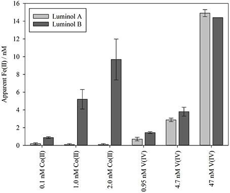
Figure 2. The maximum possible Fe(II) concentration attributable to interference from Co(II) and V(IV) spikes added to Mediterranean seawater. This was calculated by deducting the pre-spike measurement of Fe(II) concentration from the highest post-spike apparent Fe(II) measurement after adding spikes of Co(II) or V(IV). The 14.4 nM apparent Fe(II) peak from 47 nM V(IV) was above the calibrated range (up to 12 nM) of the luminol B method.

Voltammetry

During the method comparison experiments, within-sample replicates from the voltammetry method were quite variable (e.g., in experiment 5 up to 20%, Table 2). This was likely a result of the high apparent reactive Fe(III) concentration observed after the addition of the Fe(II) spike. Furthermore, it is difficult to explain the large increase in Fe_R observed post Fe(II) spike, but these Fe_R concentrations resulted in problems of carry-over and reproducibility for the voltammetry method. Fe(II) concentrations estimated by voltammetry decreased after the first time point to below detection, with the exception of experiment 4 (Figure 1D). The voltammetry method thus agreed with the results obtained from the luminol methods, except when riverine NOM was present. The depleted O₂ content of the experimental seawater was likely a contributing factor to the instability of Fe_R, as the dissolved O₂ content of sampled water likely increased between sample collection and Fe_R measurement, and was not necessarily constant between replicate sub-samples for Fe_R.

Ferrozine

The ferrozine method produced data with a temporal resolution similar to that of the luminol B method. Approximately 5 min was required to complete analysis of a sample and flush the LWCC prior to loading the next sample. For the method comparison experiments (Table 1), initial Fe(II) concentrations of 31–151% [Fe(II)]_t0 were obtained using the ferrozine method. The lowest recovery of the calculated spike added at the first sampled time point (31%) was for experiment 4 (Figure 1D), where a fulvic/humic spike was added, and this recovery was indeed the lowest for any method in any experiment (the recovery range without this experiment was 72 to 153%). Observed Fe(II) concentrations using the ferrozine method never declined to below the detection limit (0.3–0.4 nM, Table 3) in any experiment. An apparently stable nanomolar Fe(II) concentration was found in experiments using coastal seawater (Figures 1A–C), in experiments using post-mesocosm water (Figures 1D–H) and also in experiments using aged river water (Figure 3).

FIGURE 3

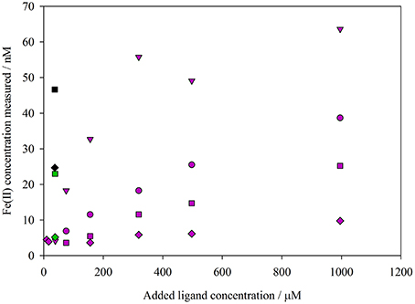
Figure 3. Comparison of Fe(II) concentrations in aged river water determined spectrophotometrically using the synthetic ligands ferrozine (purple), ferene (green), and TPTZ (black). A varying ligand concentration, and time interval between ligand addition and absorbance measurement (diamonds 2 min, squares 80 min, circles 140 min, triangles 20 h), was used.

Comparison of Synthetic Fe(II) Ligands in Riverwater

A comparison of different Fe(II) binding ligands used for spectrophotometric Fe(II) analysis suggested that all three ligand-Fe(II) methods reported a low nanomolar, stable Fe(II) concentration in aged river water (Figure 3). The observed Fe(II) concentration using the ferrozine method increased both with ferrozine concentration, and with increased time between ferrozine addition and absorbance measurement (Figure 3).

Discussion

Derivation of Apparent Oxidation Rate Constants

The results presented here show that Fe(II) is an extremely transient species which is analytically challenging to quantify in seawater. During method comparison experiments in coastal seawater, where the concentration of Fe(II) declined due to rapid oxidation (Figure 1), it was difficult to directly compare individual datapoints for each method as they were subject to small offsets in measurement and/or sample timing. Even for the two FIA luminol methods, used here with automated timing, there was a non-negligible time difference comparing direct injection (luminol A) with pre-concentration (luminol B), which had implications for how the measured Fe(II) concentrations were interpreted. A qualitative comparison of datapoints from the different analytical techniques could be made visually (Figure 1). A more robust quantitative comparison, which should not be affected by a small measurement time offset, was made by deriving the apparent oxidation rate constant of Fe(II) oxidation (Equation 1).

The apparent oxidation rate of nanomolar Fe(II) concentrations in seawater (Equations 1 and 2) is assumed to be first order with respect to the concentration of Fe(II) (Millero et al., 1987; Santana-Casiano et al., 2005), and thus the apparent rate constant k₁ (s⁻¹) was derived from the gradient of a plot of ln[(Fe(II)] against time (e.g., Figure 4). The measured decline in Fe(II) concentration (Figure 1) following spikes of Fe(II) to seawater should approximate the oxidation rate, because oxidation is anticipated to be the dominant Fe(II) removal process under these experimental conditions (Table 2).

FIGURE 4

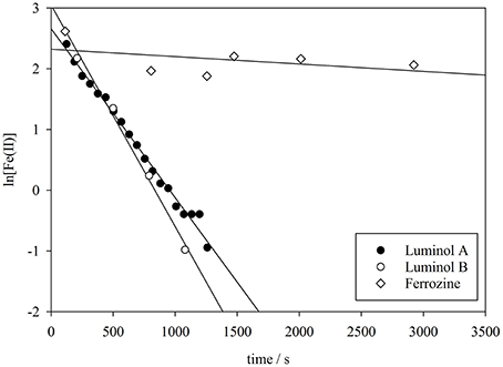
Figure 4. The derivation of the pseudo-first order oxidation rate constant (k₁) from luminol A, luminol B, and ferrozine observed Fe(II) concentrations in method comparison experiment 3.

The voltammetry determined Fe(II) concentrations were subject to a large uncertainty because of the high (5.2 to 31 nM) Fe(II) spikes added. Voltammetry is not a technique ideally suited to analyses of high, or highly variable, DFe concentrations because it relies on subtracting measured Fe(III) from measured DFe [thus the propagated error for Fe(II) concentration is always larger than for a direct measurement of DFe or Fe(III)]. Also, voltammetry required an analysis time of 30 min per sample and was thereby slow compared to other available methods. Given the low temporal resolution of this data we therefore opted not to calculate k₁ for voltammetry data.

The calculated oxidation rate of Fe(II) with O₂ in experiments 1–8 (Table 4) was derived using reported rate constants determined under laboratory conditions (Millero et al., 1987) and from measurements using a luminol chemiluminescence method in surface North Pacific seawater (Roy and Wells, 2011). As discussed further in prior work (Hansard et al., 2009; Sarthou et al., 2011), there are multiple reasons why these calculated rate constants are for indicative purposes only (e.g., O₂ may have changed over the duration of the experiments, the effect of DOC is not accounted for in this simple rate equation, the contribution of H₂O₂ to the oxidation rate was likely non-negligible, and the values derived from Roy and Wells (2011) are not corrected for small discrepancies in salinity or temperature). Yet, the differences between the luminol and ferrozine based methods are striking nonetheless (Figure 5).

TABLE 4

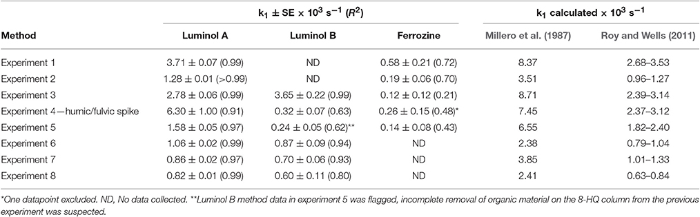
Table 4. A comparison of different methods for determining Fe(II) concentrations, which should not be affected by the measurement time offset between different methods, was made by deriving the apparent Fe(II) oxidation constant (k₁). SE, the standard error, (and R²) is also shown for the linear regression.

FIGURE 5

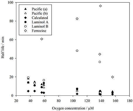
Figure 5. Comparison of Fe(II) half-life (ln(2)/k₁) derived from measurements in surface Pacific seawater (Roy and Wells, 2011), from method comparison experiments reported here, and calculated from rate constants (Millero et al., 1987).

Luminol A produced rate constants comparable to those measured (after adjusting the dissolved O₂ concentration) in surface Pacific seawater with a luminol based method (Roy and Wells, 2011) and universally smaller than those derived from Millero et al. (1987), although we note that derived constants are very sensitive to how K_w is parameterized. Luminol B was also generally comparable to the range derived from Roy and Wells (2011), except for experiments 4 and 5 (where the linear fit was notably poorer: R² 0.63 and 0.62, respectively). For the two luminol methods (A and B), although the experimentally derived apparent rate constants were never identical (even considering the modest uncertainty in k₁), k₁ was similar in experiments 3, 6, 7, and 8 (Table 4). Whereas, the discrepancy in k₁ between luminol A and ferrozine measurements was always marked. The ferrozine derived Fe(II) time series exhibited a poor linear fit and thus the relative uncertainty was always high compared to luminol A and B. Curiously though, in the humic/fulvic spiked experiment (experiment 4) the pre-concentration method (luminol B) also indicated a residual stable Fe(II) concentration, similar to the ferrozine technique. The ferrozine/luminol B derived values of k₁ were also similar for this experiment (Table 4). Between experiments 3 and 4 all conditions other than the humic/fulvic spike were similar (Table 2).

Potential Explanations for Inter-Method Differences in Fe(II) Concentration and Oxidation Rate

Lower than expected values of k₁, and correspondingly long half-lives with respect to oxidation, have been reported in various natural waters using the ferrozine method (Kieber et al., 2001; Statham et al., 2005; Klar et al., in press) with the foremost hypothesis to explain this phenomenon being the existence of stable Fe(II)-organic species. Whilst all methods here, consistent with data by Roy and Wells (2011), produced half-lives slower than expected based on relatively simple calculations from rate constants, ferrozine in all cases produced the longest half-lives (Figure 5). In no experiments were these half-lives similar to those derived from luminol A data.

Various drawbacks have been identified with all available Fe(II) methods. It is relatively straightforward, for example, to demonstrate that the unmodified ferrozine method appears to over-estimate nanomolar Fe(II) concentrations in some natural waters (Figure 3; Murray and Gill, 1978; Box, 1984; Cowart et al., 1993), which could be attributed to reduction of labile Fe(III) phases in the presence of NOM after the ferrozine ligand is added. Short mixing times between ferrozine addition and absorbance measurement, combined with handling samples in the dark and buffering to near-neutral pH, is reported to minimize, although not eliminate, the interference due to labile Fe(III) reduction (Box, 1984; Pullin and Cabaniss, 2001). This interference may potentially be more important when a LWCC is used at low (nM) Fe(II) concentrations because of the more intense light source required as part of this apparatus. The contribution of light-exposure during analysis to a supposed overestimation of Fe(II) concentration cannot alone however explain the increase in measured Fe(II) concentrations in aged river water when the time interval between ferrozine addition and absorbance measurement was increased (Figure 3).

Conversely, the binding of Fe(II) to NOM could lead to an underestimation of Fe(II) concentration by the ferrozine method when a short mixing time is used due to slow complexation of organically associated Fe(II) (Kieber et al., 2005; Hopwood et al., 2014). This issue appears however to be confined exclusively to freshwater environments as there is presently no conclusive evidence that sufficiently strong Fe(II)-NOM interactions exist in seawater to impede complexation of Fe(II) by addition of a synthetic ligand (Croot and Hunter, 2000).

Ferrozine derived Fe(II) results in the method comparison experiments (Figure 1) were therefore generally consistent with the known limitations of the unmodified ferrozine method in natural waters. The first datapoints were generally in agreement with the initial spike of Fe(II) added, confirming that the later over-estimation of Fe(II) could not consistently be attributed to an erroneous baseline. It remains possible that the residual Fe(II) concentration observed at the end of all experiments by ferrozine, and occasionally luminol B, (Figure 1) represents an Fe(II)-species which is resistant to oxidation, and indeed the presence of organic compounds capable of retarding Fe(II) oxidation in seawater has been widely discussed in prior work (e.g., González et al., 2014; Santana-Casiano et al., 2014). However, it is not expected that such high residual Fe(II) concentrations (2.7–9.1 nM) would remain in aged Mediterranean seawater. Furthermore, such stable Fe(II) species should, in principle, be detected by all analytical approaches.

Non-linearity in plots of ln[Fe(II)] against time, as observed for ferrozine Fe(II) data here (e.g., Figure 4), is often observed at low nanomolar Fe(II) concentrations, as under these conditions the assumption of a first order rate with respect to Fe(II) concentration does not appear to be universally correct (King et al., 1995; Santana-Casiano et al., 2006). However, here the non-linearity was much more pronounced using the ferrozine method. Yet it is not clear why such a large difference arises in both Fe(II) concentrations and k₁ between the ferrozine and luminol A method. Comparison of ferrozine with other synthetic ligands added to aged alkaline river water suggested that an increase in measured Fe(II) is to be expected with time whenever a strong Fe(II) ligand is added as part of a spectrophotometric method. It should however be noted that the rates of increase in measured Fe(II) concentration reported here (Figure 3) are likely not representative of all experimental conditions or all natural waters. The change in Fe(II) concentration after the addition of a synthetic Fe(II) ligand to natural water may be very sensitive to the type(s) of NOM present in solution, and thus experiments with river water and IHSS humic/fulvic additions are not directly comparable to experiments with additions of marine derived NOM. No attempt was made to optimize the methods for ferene and TPTZ to minimize the observed increase in Fe(II) concentration [the methods were used simply as previously described (Collins and Diehl, 1960; Hennessy et al., 1984)] and thus nor should the comparison (Figure 3) be interpreted as demonstrating that the overestimation of Fe(II) concentration is consistently greater when using ferene or TPTZ instead of ferrozine.

Results from Fe(II) method comparison experiment 4 (Figure 1D) suggested that terrestrially derived NOM can impact the determination of Fe(II) concentrations in a number of different ways. Terrestrially derived NOM is known to contain Fe(III) chelators (Powell and Wilson-Finelli, 2003; Krachler et al., 2005), and suggested to contain Fe(II) chelators (Kieber et al., 2005; Statham et al., 2012), that result in the formation of relatively stable complexes and/or colloids. Dissolved organic Fe(II) species, with retarded Fe(II) oxidation rates relative to inorganic Fe(II), could therefore be formed by the addition of humic/fulvic compounds to seawater. Yet the addition of strong Fe(III) chelators into solution would be expected to facilitate Fe(II) oxidation (Boukhalfa and Crumbliss, 2002; Ussher et al., 2005) and indeed the acceleration of Fe(II) oxidation in seawater by NOM is used to explain faster than expected rates of decay observed in seawater. The formation of Fe(II)-organic species could possibly change the recovery of Fe(II) by the different methods employed, for example by altering the retention efficiency of Fe(II) on the 8-HQ column used in luminol B (Ussher et al., 2005) and this could produce bias in the derived oxidation rate. Also, as evidenced by a change in detection limit (Table 3), the chemiluminescence produced by luminol is generally suppressed by humic/fulvic material (Rose and Waite, 2001).

In experiment 4, luminol A was the only method to determine that Fe(II) concentrations fell below the detection limit (0.49 nM for luminol A) with an apparent rate constant greater than in any other experiment (the standard error on k₁ was also disproportionately high). This could, in isolation, be interpreted as an acceleration of the Fe(II) oxidation rate in the presence of NOM. However, we must also consider the consistent order of magnitude difference in k₁ derived from luminol A and ferrozine. In method comparison experiment 4, luminol B, voltammetry and ferrozine methods consistently observed a stable, >4 nM concentration of Fe(II) in solution for over 30 min after the addition of an Fe(II) spike. The only clear distinction between these three methods collectively and luminol A, is that luminol B, ferrozine and voltammetry all work via the complexation of Fe(II) to a ligand (8-HQ, ferrozine and Dp, respectively) whereas luminol A relies on only the catalytic effect of Fe(II) reacting with luminol. It remains a possibility that, on the timescale of the comparison experiments (0.5–1 h), the development of Fe(II)-organic species contributes to a retarded oxidation rate. However, because the effect of organic material is method-dependent, it is also apparent that there is at least one method interference related to the presence of the added NOM. Whilst Fe(III)-organic speciation in seawater is at least moderately well-defined on a global scale (see, for example, Gledhill and Buck, 2012), Fe(II)-organic speciation in natural waters is almost entirely uncharacterized and, as we demonstrate here, is difficult to probe with existing methods which can exhibit conflicting results even in quite simple experiments. Thus, it is very difficult to evaluate if Fe(II)-organic species are present as a significant fraction of measured Fe(II) concentrations in natural waters and to assess the potential artifacts of any such Fe(II)-organic species on the accuracy of Fe(II) measurements. More generally, it is difficult to unambiguously confirm the classic interpretation for discrepancies in Fe(II) oxidation rates in natural waters; that faster than expected Fe(II) oxidation rates are driven by fractions of NOM (e.g., Roy and Wells, 2011; Lee et al., 2017), whereas slower than expected Fe(II) oxidation rates are driven by a fraction of Fe(II) present as stable Fe(II)-organic species (e.g., Willey et al., 2005; Klar et al., in press); when contradictory conclusions are drawn from two independent methods in the same series of experiments.

Limitations to Analysis of Fe(II) Concentration in Seawater

With FIA for the determination of total DFe in seawater (an analytical method for which it is possible to verify the accuracy of measurements) a mathematical approach shows that the determination of the correct gradient for a calibration curve is the single greatest error in the determination of DFe concentrations (Floor et al., 2015). For Fe(II) measurement via FIA using standard addition of Fe(II), this is therefore also very likely to be the case. Here each Fe(II) method was independently calibrated for each experiment and thus differences may have arisen because of random errors when comparing k₁ for luminol A and B. The relatively high detection limit for luminol B (Table 3) compared to luminol A partially arose because the pre-concentration system (luminol B) was optimized for low, or sub-, nanomolar concentrations. However, it is curious that whilst the interference for V(IV) was similar for both methods, the interference from Co(II) was more pronounced for the luminol B method (Figure 2). This was unexpected as the added DMG is known to suppress this interference (Ussher et al., 2009). It was suspected that the DMG decomposed during transport as several months previously the same batch was used successfully.

A specific difficulty arises when calibrating the Fe(II) FIA methods at intermediate O₂ concentrations where Fe(II) is oxidizing as it is analyzed. Unless a standard addition of Fe(II) is made internally, exactly as the luminol reagent and seawater mix, the concentration of Fe(II) entering the FIA sample line should always be greater than the concentration of Fe(II) that enters the flow cell as luminescence is produced. Calibrating the method by standard addition into the same matrix as the samples via the same loading procedure thereby means that standard peaks decline as spiked solutions are run. For standard additions, the rate of decline of an Fe(II) spike should be identical to the rate of decline of Fe(II) in a sample- assuming that the sample matrix is non-changeable and ignoring possible complications due to hypothesized Fe(II)-organic species. Yet in reality the sample matrix cannot be maintained at its exact initial condition with respect to dissolved O₂ unless it is either practically anoxic (in which case it can theoretically be maintained in its ambient state with a flow of inert gas), or at equilibrium with atmospheric O_2. At intermediate O₂ concentrations, the dissolved O₂ content of a sample is likely to increase as it is analyzed increasing the Fe(II) oxidation rate. The alternative approach is running standard solutions with a stable concentration of Fe(II) (for example, as per the luminol B method, using a low pH standard matrix) (Hansard and Landing, 2009). In this case, the rate of decay of Fe(II) in the sample as it is analyzed is not accounted for. Yet, the calibration slope is likely subject to less uncertainty. It is not clear which is preferable from an analytical perspective.

Implications for Best Practice in Fe(II) Analysis

Inter-study differences in how Fe(II) methods are calibrated appears to remain a minor issue compared to the apparent difference reported here between the ferrozine and luminol observed Fe(II) concentrations and k₁. It is yet to be established why, and under what circumstances, significant inter-method differences arise between absolute measurements of Fe(II) concentration and apparent oxidation rates. Whilst the accuracy of DFe measurements can be verified by analysis of a reference material, the transient nature of Fe(II) means that such a simple and robust verification of dissolved Fe(II) concentrations is not possible and thus greater uncertainty is generally acknowledged in Fe(II) concentrations. Yet changes in Fe(II) oxidation rate in natural waters are widely assumed to be a robust indicator of changes in Fe(II) speciation. Here, we suggest that Fe(II) oxidation rates in natural waters can be method-dependent and thus caution should be used when comparing apparent rate constants derived from different methods, especially across gradients in NOM and more generally between different sample matrixes. Process studies in natural waters using k₁/half-life as an indicator of Fe(II) speciation should ideally demonstrate that the analytical methods used produce the expected decay rate of Fe(II) spikes to an aged sample matrix with environmentally relevant concentrations of Fe(II) added. As is already often the case (e.g., Sarthou et al., 2011), Fe(II) methods should also be frequently recalibrated using the most appropriate sample matrix in order to account, as best as possible, for the effects of any shifts in the sample matrix composition on measured Fe(II) concentration and oxidation rate.

Conclusions

The almost universal adaptation of a luminol based method for measuring Fe(II) in seawater, largely because of its sensitivity and the possibility to achieve low picomolar detection limits, means that it should be logistically feasible to standardize a precise definition of “Fe(II)”. Thus, even if Fe(II) was measured with unknown accuracy and not all interfering species or method artifacts were identified, Fe(II) data in specified environments would at least be internally consistent and precision could be improved. Such standardization has however yet to occur as at present there are methodological differences reported in sample handling, preservation and analysis techniques. Fortunately, whilst some uncertainties remain with respect to interfering species, it seems that different luminol FIA techniques produce similar Fe(II) concentrations and apparent oxidation rates in a simple seawater matrix.

Yet here we found a consistent discrepancy between the results of the luminol and unmodified ferrozine methods both in observed Fe(II) concentrations and in apparent oxidation rate constants. This highlights the particular difficulty in measuring Fe(II) concentrations, and suggests that the uncertainty in the accuracy of Fe(II) oxidation rates with any presently available method is considerably larger than the standard error of the apparent oxidation rate constant. A safe conclusion is that deviations from expected Fe(II) oxidation rates in natural waters should be interpreted with caution as the artifacts of available Fe(II) methods are not fully understood.

Author Contributions

All authors contributed to the design of the study and interpreted the data. MH, AB, and MG conducted laboratory analysis. MH and AB wrote the initial draft of the paper and then all authors contributed to its revision.

Funding

Analytical work in Crete was funded by the European Commission (OCEAN-CERTAIN, FP7- ENV-2013-6.1-1; no: 603773). MH, MG, and EA gratefully acknowledge funding from the Collaborative Research Centre 754 (SFB 754) “Climate-Biogeochemistry Interactions in the Tropical Ocean” funded by the German Research Foundation (DFG).

Conflict of Interest Statement

The authors declare that the research was conducted in the absence of any commercial or financial relationships that could be construed as a potential conflict of interest.

Acknowledgments

D. Polyviou (University of Southampton) is thanked for H₂O₂ measurements, E. Skjoldal (University of Bergen) for O₂ measurements, E. Reggiani (NIVA) for carbonate measurements and J. Gallego-Urrea (University of Gothenburg) for assistance with CO2SYS. M. Rijkenberg (NIOZ) is thanked for recommendations on calibration methods for Fe(II) FIA. Labview software for operating the luminol A FIA system was designed by P. Croot, M. Heller, C. Neill, and W. King. Linear regression (and standard errors) were calculated in SigmaPlot.

Supplementary Material

The Supplementary Material for this article can be found online at: https://www.frontiersin.org/article/10.3389/fmars.2017.00192/full#supplementary-material

References

Barbeau, K. (2006). Photochemistry of organic iron(III) complexing ligands in oceanic systems. Photochem. Photobiol. 82, 1505–1516. doi: 10.1111/j.1751-1097.2006.tb09806.x

PubMed Abstract | CrossRef Full Text | Google Scholar

Boukhalfa, H., and Crumbliss, A. L. (2002). Chemical aspects of siderophore mediated iron transport. Biometals 15, 325–339. doi: 10.1023/A:1020218608266

PubMed Abstract | CrossRef Full Text | Google Scholar

Bowie, A. R., Achterberg, E. P., Sedwick, P. N., Ussher, S., and Worsfold, P. J. (2002). Real-time monitoring of picomolar concentrations of iron(II) in marine waters using automated flow injection-chemiluminescence instrumentation. Environ. Sci. Technol. 36, 4600–4607. doi: 10.1021/es020045v

PubMed Abstract | CrossRef Full Text | Google Scholar

Box, J. D. (1984). Observations on the use of iron(II) complexing agents to fractionate the total filterable iron in natural-water samples. Water Res. 18, 397–402. doi: 10.1016/0043-1354(84)90146-5

CrossRef Full Text | Google Scholar

Chin, C. S., Coale, K. H., Elrod, V. A., Johnson, K. S., Massoth, G. J., and Baker, E. T. (1994). In-Situ observations of dissolved iron and manganese in hydrothermal vent plumes, Juan-De-Fuca Ridge. J. Geophys. Res. Earth 99, 4969–4984. doi: 10.1029/93JB02036

CrossRef Full Text | Google Scholar

Collins, P., and Diehl, H. (1960). Tripyridyltriazine, a reagent for the determination of iron in sea water. J. Mar. Res 18, 152–156.

Cowart, R. E., Singleton, F. L., and Hind, J. S. (1993). A comparison of bathophenanthrolinedisulfonic acid and ferrozine as chelators of iron(II) in reduction reactions. Anal. Biochem. 211, 151–155. doi: 10.1006/abio.1993.1246

PubMed Abstract | CrossRef Full Text | Google Scholar

Croot, P. L., Bluhm, K., Schlosser, C., Streu, P., Breitbarth, E., Frew, R., et al. (2008). Regeneration of Fe(II) during EIFeX and SOFeX. Geophys. Res. Lett. 35:L19606. doi: 10.1029/2008GL035063

CrossRef Full Text | Google Scholar

Croot, P. L., Bowie, A. R., Frew, R. D., Maldonado, M. T., Hall, J. A., Safi, K. A., et al. (2001). Retention of dissolved iron and Fe-II in an iron induced Southern Ocean phytoplankton bloom. Geophys. Res. Lett. 28, 3425–3428. doi: 10.1029/2001GL013023

CrossRef Full Text | Google Scholar

Croot, P. L., and Hunter, K. A. (2000). Determination of Fe(II) and total iron in natural waters with 3-(2-pyridyl)-5,6-diphenyl-1,2,4-triazin (PDT). Anal. Chim. Acta 406, 289–302. doi: 10.1016/S0003-2670(99)00758-8

CrossRef Full Text | Google Scholar

Croot, P. L., and Laan, P. (2002). Continuous shipboard determination of Fe(II) in polar waters using flow injection analysis with chemiluminescence detection. Anal. Chim. Acta 466, 261–273. doi: 10.1016/S0003-2670(02)00596-2

CrossRef Full Text | Google Scholar

Davison, W., and Seed, G. (1983). The kinetics of the oxidation of ferrous iron in synthetic and natural-waters. Geochim. Cosmochim. Acta 47, 67–79. doi: 10.1016/0016-7037(83)90091-1

CrossRef Full Text | Google Scholar

Emmenegger, L., Schonenberger, R. R., Sigg, L., and Sulzberger, B. (2001). Light-induced redox cycling of iron in circumneutral lakes. Limnol. Oceanogr. 46, 49–61. doi: 10.4319/lo.2001.46.1.0049

CrossRef Full Text | Google Scholar

Farmer, C. T., and Hansell, D. H. (2007). “Determination of dissolved organic carbon and total dissolved nitrogen in sea water,” in Guide to Best Practices for Ocean CO2 Measurements, eds A. G. Dickson, C. L. Sabine, and J. R. Christian (PICES Special Publication 3), 191.

Floor, G. H., Clough, R., Lohan, M. C., Ussher, S. J., Worsfold, P. J., and Quétel, C. R. (2015). Combined uncertainty estimation for the determination of the dissolved iron amount content in seawater using flow injection with chemiluminescence detection. Limnol. Oceanogr. Methods 13, 673–686. doi: 10.1002/lom3.10057

PubMed Abstract | CrossRef Full Text | Google Scholar

Gledhill, M., and Buck, K. N. (2012). The organic complexation of iron in the marine environment: a review. Front. Microbiol. 3:69. doi: 10.3389/fmicb.2012.00069

PubMed Abstract | CrossRef Full Text | Google Scholar

Gledhill, M., and Van Den Berg, C. M. G. (1995). Measurement of the redox speciation of iron in seawater by catalytic cathodic stripping voltammetry. Mar. Chem. 50, 51–61. doi: 10.1016/0304-4203(95)00026-N

CrossRef Full Text | Google Scholar

González, A. G., Santana-Casiano, J. M., González-Dávila, M., Pérez-Almeida, N., and Suárez de Tangil, M. (2014). Effect of Dunaliella tertiolecta organic exudates on the Fe(II) oxidation kinetics in seawater. Environ. Sci. Technol. 48, 7933–7941. doi: 10.1021/es5013092

PubMed Abstract | CrossRef Full Text | Google Scholar

Hansard, S. P., and Landing, W. M. (2009). Determination of iron(II) in acidified seawater samples by luminol chemiluminescence. Limnol. Oceanogr. 7, 222–234. doi: 10.4319/lom.2009.7.222

CrossRef Full Text | Google Scholar

Hansard, S. P., Landing, W. M., Measures, C. I., and Voelker, B. M. (2009). Dissolved iron(II) in the Pacific Ocean: measurements from the PO2 and P16N CLIVAR/CO2 repeat hydrography expeditions. Deep. Res. Part I-Oceanographic Res. Pap. 56, 1117–1129. doi: 10.1016/j.dsr.2009.03.006

CrossRef Full Text | Google Scholar

Hennessy, D. J., Reid, G. R., Smith, F. E., and Thompson, S. L. (1984). Ferene - a new spectrophotometric reagent for iron. Can. J. Chem. Can. Chim. 62, 721–724. doi: 10.1139/v84-121

CrossRef Full Text | Google Scholar

Hong, H., and Kester, D. R. (1986). Redox state of iron in the offshore waters of Peru. Limnol. Oceanogr. 31, 512–524. doi: 10.4319/lo.1986.31.3.0512

CrossRef Full Text | Google Scholar

Hopwood, M. J., Statham, P. J., and Milani, A. (2014). Dissolved Fe(II) in a river-estuary system rich in dissolved organic matter. Estuar. Coast. Shelf Sci. 151, 1–9. doi: 10.1016/j.ecss.2014.09.015

CrossRef Full Text | Google Scholar

Hopwood, M. J., Statham, P. J., Skrabal, S. A., and Willey, J. D. (2015). Dissolved iron(II) ligands in river and estuarine water. Mar. Chem. 173, 173–182. doi: 10.1016/j.marchem.2014.11.004

CrossRef Full Text | Google Scholar

Kieber, R. J., Skrabal, S. A., Smith, B. J., and Willey, J. D. (2005). Organic complexation of Fe(II) and its impact on the redox cycling of iron in rain. Environ. Sci. Technol. 39, 1576–1583. doi: 10.1021/es040439h

PubMed Abstract | CrossRef Full Text | Google Scholar

Kieber, R. J., Williams, K., Willey, J. D., Skrabal, S., and Avery, G. B. (2001). Iron speciation in coastal rainwater: concentration and deposition to seawater. Mar. Chem. 73, 83–95. doi: 10.1016/S0304-4203(00)00097-9

CrossRef Full Text | Google Scholar

King, D. W., Lounsbury, H. A., and Millero, F. J. (1995). Rates and mechanism of Fe(II) oxidation at nanomolar total iron concentrations. Environ. Sci. Technol. 29, 818–824. doi: 10.1021/es00003a033

PubMed Abstract | CrossRef Full Text | Google Scholar

Klar, J. K., Homoky, W. B., Statham, P. J., Birchill, A. J., Harris, E. L., Woodward, E. M. S., et al. (in press). Stability of dissolved and soluble Fe(II) in shelf sediment pore waters and release to an oxic water column. Biogeochemistry. doi: 10.1007/s10533-017-0309-x

CrossRef Full Text | Google Scholar

Krachler, R., Jirsa, F., and Ayromlou, S. (2005). Factors influencing the dissolved iron input by river water to the open ocean. Biogeosciences 2, 311–315. doi: 10.5194/bg-2-311-2005

CrossRef Full Text | Google Scholar

Kuma, K., Katsumoto, A., Nishioka, J., and Matsunaga, K. (1998). Size-fractionated iron concentrations and Fe(III) hydroxide solubilities in various coastal waters. Estuar. Coast. Shelf Sci. 47, 275–283. doi: 10.1006/ecss.1998.0355

CrossRef Full Text | Google Scholar

Lee, Y. P., Fujii, M., Kikuchi, T., Natsuike, M., Ito, H., Watanabe, T., et al. (2017). Importance of allochthonous and autochthonous dissolved organic matter in Fe(II) oxidation: a case study in Shizugawa Bay watershed, Japan. Chemosphere 180, 221–228. doi: 10.1016/j.chemosphere.2017.04.008

PubMed Abstract | CrossRef Full Text | Google Scholar

Lin, H., and Twining, B. S. (2012). Chemical speciation of iron in Antarctic waters surrounding free-drifting icebergs. Mar. Chem. 128, 81–91. doi: 10.1016/j.marchem.2011.10.005

CrossRef Full Text | Google Scholar

Lohan, M. C., and Bruland, K. W. (2008). Elevated Fe(II) and dissolved Fe in hypoxic shelf waters off Oregon and Washington: an enhanced source of iron to coastal upwelling regimes. Environ. Sci. Technol. 42, 6462–6468. doi: 10.1021/es800144j

PubMed Abstract | CrossRef Full Text | Google Scholar

Mawji, E., Schlitzer, R., Dodas, E. M., Abadie, C., Abouchami, W., Anderson, R. F., et al. (2015). The GEOTRACES intermediate data product 2014. Mar. Chem. 177, 1–8. doi: 10.1016/j.marchem.2015.04.005

CrossRef Full Text | Google Scholar

Millero, F. J. (1998). Solubility of Fe(III) in seawater. Earth Planet. Sci. Lett. 154, 323–329. doi: 10.1016/S0012-821X(97)00179-9

CrossRef Full Text | Google Scholar

Millero, F. J., and Sotolongo, S. (1989). The oxidation of Fe(II) with H₂O₂ in seawater. Geochim. Cosmochim. Acta 53, 1867–1873. doi: 10.1016/0016-7037(89)90307-4

CrossRef Full Text | Google Scholar

Millero, F. J., Sotolongo, S., and Izaguirre, M. (1987). The oxidation-kinetics of Fe(II) in seawater. Geochim. Cosmochim. Acta 51, 793–801. doi: 10.1016/0016-7037(87)90093-7

CrossRef Full Text | Google Scholar

Millero, F. J., Yao, W., and Aicher, J. (1995). The speciation of Fe(II) and Fe(III) in natural waters. Mar. Chem. 50, 21–39. doi: 10.1016/0304-4203(95)00024-L

CrossRef Full Text | Google Scholar

Murray, J. W., and Gill, G. (1978). Geochemistry of iron in Puget Sound. Geochim. Cosmochim. Acta 42, 9–19. doi: 10.1016/0016-7037(78)90211-9

CrossRef Full Text | Google Scholar

O'Sullivan, D. W., Hanson, A. K. Jr., and Kester, D. R. (1995). Stopped flow luminol chemiluminescence determination of Fe(II) and reducible iron in seawater at subnanomolar levels. Mar. Chem. 49, 65–77.

Google Scholar

O'Sullivan, D. W., Hanson, A. K. Jr., Miller, W. L., and Kester, D. R. (1991). Measurement of Fe(II) in Surface water of the Equatorial Pacific. Limnol. Oceanogr. 36, 1727–1741.

Google Scholar

Powell, R. T., and Wilson-Finelli, A. (2003). Importance of organic Fe complexing ligands in the Mississippi River plume. Estuar. Coast. Shelf Sci. 58, 757–763. doi: 10.1016/S0272-7714(03)00182-3

CrossRef Full Text | Google Scholar

Pullin, M. J., and Cabaniss, S. E. (2001). Colorimetric flow-injection analysis of dissolved iron in high DOC waters. Water Res. 35, 363–372. doi: 10.1016/S0043-1354(00)00259-1

PubMed Abstract | CrossRef Full Text | Google Scholar

Redfield, A. C. (1934). “On the proportions of organic derivations in sea water and their relation to the composition of plankton,” in James Johnstone Memorial Volume, ed R. J. Daniel (Liverpool: University Press of Liverpool), 177–192.

Google Scholar

Rose, A. L., and Waite, T. D. (2001). Chemiluminescence of luminol in the presence of iron(II) and oxygen: oxidation mechanism and implications for its analytical use. Anal. Chem. 73, 5909–5920. doi: 10.1021/ac015547q

PubMed Abstract | CrossRef Full Text | Google Scholar

Rose, A. L., and Waite, T. D. (2002). Kinetic model for Fe(II) oxidation in seawater in the absence and presence of natural organic matter. Environ. Sci. Technol. 36, 433–444. doi: 10.1021/es0109242

PubMed Abstract | CrossRef Full Text | Google Scholar

Rose, A. L., and Waite, T. D. (2003). Effect of dissolved natural organic matter on the kinetics of ferrous iron oxygenation in seawater. Environ. Sci. Technol. 37, 4877–4886. doi: 10.1021/es034152g

PubMed Abstract | CrossRef Full Text | Google Scholar

Roy, E. G., and Wells, M. L. (2011). Evidence for regulation of Fe(II) oxidation by organic complexing ligands in the Eastern Subarctic Pacific. Mar. Chem. 127, 115–122. doi: 10.1016/j.marchem.2011.08.006

CrossRef Full Text | Google Scholar

Santana-Casiano, J. M., Gonzaalez-Davila, M., and Millero, F. J. (2005). Oxidation of nanomolar levels of Fe(II) with oxygen in natural waters. Environ. Sci. Technol. 39, 2073–2079. doi: 10.1021/es049748y

PubMed Abstract | CrossRef Full Text | Google Scholar

Santana-Casiano, J. M., Gonzalez-Davila, A., and Millero, F. J. (2006). The role of Fe(II) species on the oxidation of Fe(II) in natural waters in the presence of O₂ and H₂O₂. Mar. Chem. 99, 70–82. doi: 10.1016/j.marchem.2005.03.010

CrossRef Full Text | Google Scholar

Santana-Casiano, J. M., Gonzalez-Davila, M., Gonzalez, A. G., Rico, M., Lopez, A., and Martel, A. (2014). Characterization of phenolic exudates from Phaeodactylum tricornutum and their effects on the chemistry of Fe(II)-Fe(III). Mar. Chem. 158, 10–16. doi: 10.1016/j.marchem.2013.11.001

CrossRef Full Text | Google Scholar

Santana-Casiano, J. M., Gonzalez-Davila, M., Rodriguez, M. J., and Millero, F. J. (2000). The effect of organic compounds in the oxidation kinetics of Fe(II). Mar. Chem. 70, 211–222. doi: 10.1016/S0304-4203(00)00027-X

CrossRef Full Text | Google Scholar

Sarradin, P. M., Le Bris, N., Le Gall, C., and Rodier, P. (2005). Fe analysis by the ferrozine method: adaptation to FIA towards in situ analysis in hydrothermal environment. Talanta 66, 1131–1138. doi: 10.1016/j.talanta.2005.01.012

PubMed Abstract | CrossRef Full Text | Google Scholar

Sarthou, G., Bucciarelli, E., Chever, F., Hansard, S. P., Gonzalez-Davila, M., Santana-Casiano, J. M., et al. (2011). Labile Fe(II) concentrations in the Atlantic sector of the Southern Ocean along a transect from the subtropical domain to the Weddell Sea Gyre. Biogeosciences 8, 2461–2479. doi: 10.5194/bg-8-2461-2011

CrossRef Full Text | Google Scholar

Sedwick, P. N., Sohst, B. M., Ussher, S. J., and Bowie, A. R. (2015). A zonal picture of the water column distribution of dissolved iron(II) during the U.S. GEOTRACES North Atlantic transect cruise (GEOTRACES GA03). Deep Sea Res. Part II Top. Stud. Oceanogr. 116, 166–175. doi: 10.1016/j.dsr2.2014.11.004

CrossRef Full Text | Google Scholar

Seitz, W. R., and Hercules, D. M. (1972). Determination of trace amounts of iron(II) using chemiluminescence analysis. Anal. Chem. 44, 2143–2149. doi: 10.1021/ac60321a020

CrossRef Full Text | Google Scholar

Smith, G. F., McCurdy, W. H., and Diehl, H. (1952). The colorimetric determination of iron in raw and treated municipal water supplies by use of 4:7-diphenyl-1:10-phenanthroline. Analyst 77, 418–422. doi: 10.1039/an9527700418

CrossRef Full Text | Google Scholar

Statham, P. J., German, C. R., and Connelly, D. P. (2005). Iron(II) distribution and oxidation kinetics in hydrothermal plumes at the Kairei and Edmond vent sites, Indian Ocean. Earth Planet. Sci. Lett. 236, 588–596. doi: 10.1016/j.epsl.2005.03.008

CrossRef Full Text | Google Scholar

Statham, P. J., Jacobson, Y., and van den Berg, C. M. G. (2012). The measurement of organically complexed Fe-II in natural waters using competitive ligand reverse titration. Anal. Chim. Acta 743, 111–116. doi: 10.1016/j.aca.2012.07.014

CrossRef Full Text | Google Scholar

Stookey, L. L. (1970). Ferrozine- a new spectrophotometric reagent for iron. Anal. Chem. 42, 779–781. doi: 10.1021/ac60289a016

CrossRef Full Text | Google Scholar

Sunda, W. G., Buffle, J., and Van Leeuwen, H. P. (2001). “Bioavailability and Bioaccumulation of Iron in the Sea,” in The Biogeochemistry of Iron in Seawater, eds D. R. Turner and K. A. Hunter (Chichester: John Wiley & Sons, Ltd.), 41–84.

Tynan, E., Clarke, J. S., Humphreys, M. P., Ribas-Ribas, M., Esposito, M., Rérolle, V. M. C., et al. (2016). Physical and biogeochemical controls on the variability in surface pH and calcium carbonate saturation states in the Atlantic sectors of the Arctic and Southern Oceans. Deep Sea Res. Part II Top. Stud. Oceanogr. 127, 7–27. doi: 10.1016/j.dsr2.2016.01.001

CrossRef Full Text | Google Scholar

Ussher, S. J., Milne, A., Landing, W. M., Attiq-ur-Rehman, K., Seguret, M. J. M., Holland, T., et al. (2009). Investigation of iron(II) reduction and trace metal interferences in the determination of dissolved iron in seawater using flow injection with luminol chemiluminescence detection. Anal. Chim. Acta 652, 259–265. doi: 10.1016/j.aca.2009.06.011

CrossRef Full Text | Google Scholar

Ussher, S. J., Worsfold, P. J., Achterberg, E. P., Laes, A., Blain, S., Laan, P., et al. (2007). Distribution and redox speciation of dissolved iron on the European continental margin. Limnol. Oceanogr. 52, 2530–2539. doi: 10.4319/lo.2007.52.6.2530

CrossRef Full Text | Google Scholar

Ussher, S. J., Yaqoob, M., Achterberg, E. P., Nabi, A., and Worsfold, P. J. (2005). Effect of model ligands on iron redox speciation in natural waters using flow injection with luminol chemiluminescence detection. Anal. Chem. 77, 1971–1978. doi: 10.1021/ac048850a

PubMed Abstract | CrossRef Full Text | Google Scholar

van Heuven, S., Pierrot, D., Rae, J. W. B., Wallace, D. W. R., and Lewis, E. (2011). MATLAB Program Developed for CO₂ System Calculations. ORNL Environmental Sciences Division ORNL/CDIAC-105b.

Vedamati, J., Goepfert, T., and Moffett, J. W. (2014). Iron speciation in the eastern tropical South Pacific oxygen minimum zone off Peru. Limnol. Oceanogr. 59, 1945–1957. doi: 10.4319/lo.2014.59.6.1945

CrossRef Full Text | Google Scholar

Waterbury, R. D., Yao, W., and Byrne, R. H. (1997). Long pathlength absorbance spectroscopy: trace analysis of Fe(II) using a 4.5 m liquid core waveguide. Anal. Chim. Acta 357, 99–102. doi: 10.1016/S0003-2670(97)00530-8

CrossRef Full Text | Google Scholar

Willey, J. D., Kieber, R. J., Seaton, P. J., and Miller, C. (2008). Rainwater as a source of Fe(II)-stabilizing ligands to seawater. Limnol. Oceanogr. 53, 1678–1684. doi: 10.4319/lo.2008.53.4.1678

CrossRef Full Text | Google Scholar

Willey, J. D., Whitehead, R. F., Kieber, R. J., and Hardison, D. R. (2005). Oxidation of Fe(II) in rainwater. Environ. Sci. Technol. 39, 2579–2585. doi: 10.1021/es0404522

PubMed Abstract | CrossRef Full Text | Google Scholar

Yuan, J. C., and Shiller, A. M. (1999). Determination of subnanomolar levels of hydrogen peroxide in seawater by reagent-injection chemiluminescence detection. Anal. Chem. 71, 1975–1980. doi: 10.1021/ac981357c

CrossRef Full Text | Google Scholar

Zhuang, G., Yi, Z., and Wallace, G. T. (1995). Iron(II) in rainwater, snow, and surface seawater from a coastal environment. Mar. Chem. 50, 41–50. doi: 10.1016/0304-4203(95)00025-M

CrossRef Full Text | Google Scholar