Validation and Intercomparison of Ocean Color Algorithms for Estimating Particulate Organic Carbon in the Oceans

1. Introduction

Total particulate organic carbon (POC or C_o) in the ocean is a key currency used in studies of both the biological export of carbon from the surface to the deep ocean, and the availability of food for marine organisms. The pool of POC in the ocean is relatively small (estimates include: 0.43 Pg C in the first light-attenuation depth—Gardner et al., 2006; 2.28 Pg C over a 200 m surface layer—Stramska, 2009). Despite the relative small size of the POC compartment, its components (phytoplankton, bacteria, zooplankton, and organic detritus) are responsible for large fluxes in the ocean, because of their high turnover rates. The organic tissue generated by photosynthesis in the sunlit ocean is either exported from the surface via the “biological pump” (Volk and Hoffert, 1985; Ducklow et al., 2001), transferred to higher trophic levels through the food chain, transformed into detritus, or recycled via the microbial loop, with some of it going into the pool of dissolved organic (DOC) and inorganic carbon (DIC). Organic particles are therefore involved in two important carbon fluxes in the ocean, primary production and export to either the deep ocean or the DOC and DIC pools, in addition to being an integral part of the marine food web. In addition to the components of POC arising from local sources, POC may be transported to a particular location from distant sources: for example, by currents that move POC horizontally in the ocean, or by transport of POC of terrestrial origin to the oceans by river outflow. Though POC is typically treated as a single pool, there is growing awareness of the importance of different particles, such as defined by their size, because of their variety of biogeochemical functions, and their effect on ocean optical properties. For example, it has been shown that around 40% of POC concentration in the oligotrophic regions may be associated with bacteria alone (Cho and Azam, 1990) and submicron detrital particles can also make a significant contribution to the POC pool (Mel'nikov, 1976). Similarly, relatively large particles (generally larger than a few micrometers) can play an important role in POC export (e.g., Boyd and Newton, 1995; Dall'Olmo et al., 2009). The importance of particles characteristics in determining the optical signal of POC has also been recognized.

The theoretical work of Stramski and Kiefer (1991), assuming spherical and homogenous particles, indicated that small particles can make an important contribution to the backscattering signal in the oceans. Further work has shown the impact of non-sphericity and intracellular structures on optical properties, particularly backscattering (Meyer, 1979; Kitchen and Zaneveld, 1992; Quirantes and Bernard, 2004, 2006; Clavano et al., 2007; Matthews and Bernard, 2013; Robertson Lain et al., 2017). Work by Cetinić et al. (2012) linked variation in the beam attenuation coefficient with plankton community composition, and variability in particle backscattering with changes in particle composition due to remineralization. They also highlighted how measurement artifacts might influence the observed relationships between POC and optical properties. Further work has explored separation of the phytoplankton component in POC—through both indirect (Behrenfeld et al., 2005; Kostadinov et al., 2016) and direct methods (Graff et al., 2012, 2015). The contribution of phytoplankton to the POC pool leads to the covariance between chlorophyll a concentration ([Chl]) and POC concentrations, although some scatter exists in these relationships, as a result of variability in the phytoplankton community composition, physiological factors that can affect the carbon-chlorophyll ratio in phytoplankton, and the variable contribution of substances other than phytoplankton (including detritus and bacteria) to POC (see discussion and references within Stramska and Stramski, 2005; Sathyendranath et al., 2009).

POC is readily quantifiable by filtering seawater samples, and forms a key component of many biological ocean models. However, in situ samples are expensive to collect, leading to a scarcity of data that hinders efforts to both validate ocean models and develop a complete understanding of POC dynamics. Satellite ocean color data offers the opportunity to quantify POC at the global scale on an almost daily basis. Ocean color or more specifically the water-leaving radiance and corresponding remote sensing reflectance spectra, and derived [Chl] are recognized as Essential Climate Variables (ECVs) by the Global Climate Observing System (GCOS, 2011). This is in recognition of their importance for studying various biological variables and processes in the ocean. In fact, of all the oceanic ECVs that are amenable to remote sensing, ocean color is the only one that targets a biological property. In response to the GCOS requirements, the European Space Agency (ESA) Ocean Color Climate Change Initiative (OC-CCI) has generated a time series of merged satellite products for climate research, using data from the ESA satellite sensor MERIS (MEdium spectral Resolution Imaging Spectrometer) and NASA (National Aeronautics and Space Administration) satellite sensors SeaWiFS (Sea-viewing Wide Field-of-view Sensor) and MODIS-Aqua (Moderate-resolution Imaging Spectroradiometer-Aqua). The products include the normalized remote-sensing reflectances, R_rs at SeaWiFS wavelengths and [Chl], as well as some additional inherent optical properties (IOPs) such as absorption and backscattering coefficients of phytoplankton and other particulate matter, and diffuse attenuation coefficient for downward plane irradiance, K_d at 490 nm. There is a recognized need in the user community for additional products from ocean color that deal directly with POC, including separation of the contribution of phytoplankton, and the size distribution of particles. Further, these products need to be regionally optimized and their uncertainties well characterized. Both of these requirements may be addressed via optical classification (e.g., Moore et al., 2009), whereby waters are classified according to their spectral or bio-optical properties. Optical classification allows specific algorithms to be applied to the different optical water types (resulting in a global, merged product) and provides provides a method (Moore et al., 2009; Jackson et al., in press) that can be used to calculate per pixel errors. Other methods exist: e.g., formal error propagation (Lee et al., 2010), or estimation of uncertainties based on model-observation comparison (Maritorena et al., 2010). However, the users consulted within the OC-CCI project expressed a preference for uncertainties based on comparison with in situ data (Sathyendranath et al., in press).

Remote sensing of POC through ocean color radiometry requires the exploitation of some optical signal that is associated with the material. In fact, optically, the beam attenuation coefficient of particles (c_p), particle scattering coefficient (b_p), backscattering coefficient (b_bp) and the attenuation coefficient of downward irradiance K_d are all sensitive to particle abundance (to a first order), and to particle composition (through refractive index), size, shape and internal structure. It has been demonstrated that POC is correlated with in situ c_p measured using transmissometers (Gardner et al., 1993; Bishop, 1999; Claustre et al., 1999; Stramska and Stramski, 2005), which has provided a robust optical method for measuring POC using in situ devices. Although b_p and c_p are not among the data products that are routinely retrieved from remote sensing, satellite-based algorithms exist for retrieving POC from all the optical properties listed above, as well as from remote-sensing reflectance values.

This paper compares five different algorithms for estimating POC concentrations, selected as being representative of varied approaches that are prevalent for POC retrieval from ocean-color data. Each algorithm is applied to different optical properties derived from satellite ocean color data, and each uses different formulations for linking the parameters to the POC concentration. Matchups between in situ measurements of POC and satellite ocean color allow for the validation, intercomparison of global performance, and estimation of uncertainties associated with the POC calculated using these algorithms.

2. Methods

2.1. Collation of an In situ Database

For this study, POC concentration data were collected from a number of existing databases and from individual contributors. Databases collated included PANGAEA (https://www.pangaea.de/) and SeaBASS (Werdell and Bailey, 2005), and those compiled by Martiny et al. (2014) and the Biological and Chemical Oceanography Data Management Office (BCO-DMO, USA). Further data were included from the Atlantic Meridional Transect (AMT) (including data derived from both CTD and the ship's clean water supply) and other cruises in the Southern Ocean (see a description of the Good Hope line and associated data collection in Thomalla et al., 2017). Operationally, POC is defined as all the organic carbon that is retained on GF/F filters (nominal pore size of 0.7 μm). To measure POC, samples are collected on pre-combusted (450°C) GF/F filters and dried overnight at 65°C before analysis. To remove particulate inorganic carbon, filters are acidified either by adding low-carbon HCl directly or by overnight exposure to the fumes of a concentrated HCl solution in a desiccator. Filters are then dried, packed in pre-combusted tin capsules, combusted at 960°C in an elemental analyser to convert the organic carbon in CO₂. The liberated CO₂ is finally detected by thermal conductivity (Sharp, 1974). Acetanilide is used as a standard. The procedure for applying a blank however is not always consistent across studies, and as such could be a source of bias within the data set collated here. Cetinić et al. (2012) (and references therein) have studied the consequences of different methodologies for treating POC blanks, summarizing that the effect of DOC adsorption on filters (if not accounted for with an adequate blank correction) can cause substantial bias at low POC concentrations. In the database used here, a large quantity of the samples from low POC regions (i.e., the oligotrophic gyres) are from the AMT cruise programme, where a multiple-volume intercept blank methodology is used to reduce potential bias from blanks. Where data was provided at depth, measurements were averaged over 10m to provide the “surface” value for the matchup. Optical weighting of these measurement were considered, however given the variability of the water types sampled and associated mixed layer depths, and the necessary assumptions to apply an optical model for this purpose, it was decided not to introduce additional sources of uncertainty for these data points.

2.2. Extraction of Satellite-In situ Matchups

Matchup extraction was based on the procedure developed for the OC-CCI. The daily, 4 km, sinusoidally projected OC-CCI version 2 data (Sathyendranath et al., 2016) were searched to find satellite data associated with each in situ data point. The OC-CCI data is a merged product from three sensors, each with a different overpass time. However these overpass times are generally around 12 p.m. ± 2.5 h, meaning a maximum time difference between the in situ and satellite data of <12 h. The OC-CCI data used contain all of the relevant optical and biogeochemical properties necessary for implementation of the different algorithms under consideration, as well as water class membership of each pixel which quantifies the similarities between the remote-sensing reflectance spectrum at that pixel and the characteristic mean and covariance spectra associated with each of the optical classes (Jackson et al., in press), see also the OC-CCI product user guide (http://www.esa-oceancolor-cci.org/?q=documents). The OC-CCI data were interrogated to assess the availability of data covering the latitude and longitude of the in situ data point, on the same date as the in situ data collection. If the central pixel contained valid data, the data surrounding eight pixels are also extracted from the selected data (a 3 × 3 pixel box, corresponding to a 12 km × 12 km region). The central value and the mean, median, and standard deviation, number of valid pixels out of the nine pixels, the optical class with the dominant membership, and the calculated POC products using various algorithms applied to the central and mean pixel values, are returned as output, along with the in situ data values and metadata.

2.3. Candidate Algorithms

Five different algorithms for determination of POC concentration were considered. For consistency of comparison, all algorithms were implemented using the appropriate variables from the OC-CCI product suite. Another reason for using the OC-CCI products is that a rigorous algorithm selection procedure for atmospheric correction (Müller et al., 2015) and in-water properties (Brewin et al., 2015) (including derivation of [Chl], IOPs and the diffuse attenuation coefficient), had been put in place, to ensure quality of products. Furthermore, being a merged product, OC-CCI coverage is higher than that available from single-sensor products, ensuring a higher number of match-up points with in situ data. However, we recognize that all the five candidate algorithms were initially developed, implemented and tested using other ocean-color products, and that any systematic differences between the OC-CCI products and the datasets used by the algorithm developers, could be a potential source of difference in performance. Therefore, in the description of the algorithms, we also provide details of how the algorithms were implemented in the original work.

We also note that there are differences in how the five algorithms compared here were developed and implemented in the original work. For example, two of the algorithms (algorithms A and B presented below) were derived solely from coincidentally collected in situ data, whereas Algorithm D (G06—described below) combined in situ measurements of POC and beam attenuation, with satellite-derived measurements of diffuse attenuation coefficient. Algorithms A and B are based on some 50 measurements, whereas the POC—beam attenuation coefficient relationship used in Algorithm D was based on over 3,000 measurements. Algorithm C (described below) relies on a large in situ database of [Chl] and backscattering ratio to estimate total particle scattering coefficient from particle backscattering coefficient, and then relies on an extensive literature review to find a conversion factor between particle scattering coefficient and POC. Here we use a common set of satellite data (OC-CCI) to compute POC using the different algorithms and compare the products against a common set of in situ data. Where there are differences between how the various steps in the algorithms were implemented in the original work, and how OC-CCI treated similar steps in its product generation, they are highlighted, since such differences could have potential impact on algorithm performance.

2.3.1. Algorithm A Based on Remote-Sensing Reflectance

This algorithm (designated C_o(A)) proposed by Stramski et al. (2008) uses remote-sensing reflectance at 443 and 555 nm (equation 1) as inputs, and takes the following form:

$\begin{array}{cc}{C}_o(A)(\text{mg}{\text{m}}^{-\text{3}})=203.2{\left[\frac{{\text{R}}_{\text{rs}}(443)}{{\text{R}}_{\text{rs}}(555)}\right]}^{-1.034}.& (1)\end{array}$

The model parameters were determined using some 53 pairs of co-located in situ measurements of both POC and spectral values of R_rs from oligotrophic and upwelling waters of the East Atlantic and the South Pacific. The authors have provided various fits to the models for different pairs of wavebands for R_rs and for different selections of data. The one we have used here is based on all data, and for the 443–555 waveband pair, as recommended by the authors. This algorithm is currently used by the NASA Ocean Biology Processing Group to generate the global POC data product from ocean color data. The R_rs values in the OC-CCI product suite were used as input to this algorithm for the validation exercise presented here. We note that a similar POC algorithm based on the blue-to-green reflectance ratio has been developed and validated with the data from the Southern Ocean (Allison et al., 2010). For the Southern Ocean algorithm the best fit coefficients of the power function of the same form as Equation (1) were determined to be 189.29 and -0.87. A power function was found to provide better error statistics compared with those using modified fits of those typically used in maximum band ratio algorithms for [Chl].

2.3.2. Algorithm B Based on Backscattering by Particles

This algorithm (C_o(B)), also proposed by Stramski et al. (2008) uses b_bp(555), the particulate backscattering coefficient at 555 nm (2), as input. The equation has the form:

$\begin{array}{cc}{C}_o(B)(\text{mg}{\text{m}}^{-\text{3}})=53606.7\times {\text{b}}_{\text{bp}}(555)+2.468.& (2)\end{array}$

Stramski et al. (2008) tested two approaches for calculating b_bp for the eventual determination of POC: firstly, the method of Maffione and Dana (1997) as refined by Boss and Pegau (2001) was used to derive spectral backscattering coefficient from in situ measurements of volume scattering function at 140^o. Next, using a two-step empirical approach, Stramski et al. (2008) then calculated b_bp by removing the backscattering coefficient for pure water [they used pure-water backscattering coefficients proposed by Buiteveld et al. (1994) and by Morel (1974), and reported that the difference between the measurements of b_bw was likely within the range of errors associated with the measurements themselves, and therefore did not substantially impact the performance of the algorithm for deriving POC]. Then, b_bp was empirically related to POC concentrations (Equation 2). Stramski et al. (2008) provide various fits to this equation, but the parameters selected above correspond to the results (number of observations = 54) excluding upwelling data, which provided better uncertainty metrics, and may better reflect the data within the database used here. Secondly, to provide the remote-sensing context, Stramski et al. (2008) used either a direct empirical relationship between the backscattering coefficient (b_b) and R_rs or the Quasi Analytical Algorithm (QAA) approach of Lee et al. (2002) to derive b_bp from R_rs. They found that the comparison with measured b_bp was improved considerably when an empirical correction based on their measurements of b_bp was applied to the QAA algorithm. Thus, this algorithm uses a two-step approach: first, b_bp is derived from R_rs, and then that b_bp is used in Equation (2) to calculate POC.

In the computation of OC-CCI b_bp products, the QAA model was used, along with Zhang et al. (2009) for the pure-water backscattering coefficient (Sathyendranath et al., 2016). In QAA the spectral backscattering coefficient is calculated empirically using R_rs at 440 nm and at 555 nm. A power law is then used to calculate the particle backscattering coefficients at other wavelengths given the value of the spectral backscattering coefficient and b_bp(555), estimated from an analytical relationship using R_rs(555) and the absorption coefficient (a(555)). These values of b_bp were used to compute POC in the calculations presented here, without any empirical correction. For this algorithm a linear fit provided the best error statistics in the original study of Stramski et al. (2008).

2.3.3. Algorithm C Based on both Backscattering Coefficient and Chlorophyll-a Concentration

This algorithm (C_o(C)) is based on a combination of b_bp(490) and [Chl], and was proposed by Loisel et al. (2002) (3). They derived b_bp and [Chl] from SeaWIFS data using the method of Loisel and Stramski (2000) and the OC4 algorithm (based on O'Reilly et al., 1998) respectively. They then used a relationship proposed by Twardowski et al. (2001) to compute the total particle scattering coefficient given the particle backscattering coefficient (b_bp) and [Chl] (designated B in Equation 3). They then adopted a conversion value of 400 mg C m⁻² to go from total scattering coefficient to POC concentration. Combining these steps yields the following algorithm:

$\begin{array}{cc}{C}_o(C)(\text{mg}{\text{m}}^{-\text{3}})=41666.7\times {\text{b}}_{\text{bp}}(490)\times {\text{B}}^{0.25}.& (3)\end{array}$

Algorithm C is implemented here using the Lee et al. (2002) QAA approach (for b_bp), and a more recent OC4 (v6) for [Chl].

2.3.4. Algorithm D Based on the Diffuse Attenuation Coefficient for Irradiance and Beam Attenuation Coefficient

This algorithm (C_o(D)), based on Gardner et al. (2006), uses a two-step relationship relating K_d(490) to beam attenuation coefficient for particles (c_p), and then the beam attenuation coefficient to POC:

$\begin{array}{cc}{c}_p=\exp (1.124\times \log 10(K_d(490)+1.1361)),& (4)\end{array}$

and

$\begin{array}{cc}{C}_o(D)(\text{mg}{\text{m}}^{-\text{3}})=12\times (31.7\times {\text{c}}_{\text{p}}+0.785).& (5)\end{array}$

In Gardner et al. (2006), K_d(490) is obtained from SeaWIFS data where the algorithm of Mueller (2000) is used, based on water-leaving radiances at 490 and 555 nm. Gardner et al. (2006) used an extensive database (number of observations = 3,462) of concurrent measurements of POC and beam attenuation coefficient from Atlantic, Pacific and Indian Oceans, to derive the parameters of Equations (4) and (5) empirically.

The K_d(490) values used in the comparison presented here are obtained from the OC-CCI version 2 data, which uses the method of Lee et al. (2005).

2.3.5. Algorithm E Based on Spectral Backscattering Coefficient

This algorithm (C_o(E)) was developed by Kostadinov et al. (2009) and Kostadinov et al. (2016). It correlates the slope (η) of backscattering as a function of wavelength to the slope (ξ) of the particle size distribution (PSD) that is assumed to follow a power-law. The method has three steps: firstly, η is calculated from the spectral b_bp values at 490, 510, and 555 nm extracted from the OC-CCI matchup data (for which OC-CCI uses Lee et al. (2002)). Note that in Kostadinov et al. (2009) and Kostadinov et al. (2016), b_bp is instead retrieved using the formulation of Loisel and Stramski (2000). Secondly, look-up-tables (LUTs) are used to retrieve the parameters of the PSD, namely the slope (ξ) and the differential number concentration at a reference diameter of 2 μm, (N_o), given η and b_bp at 443 nm. The LUTs are constructed using theoretical forward simulations using Mie code (Bohren and Huffman, 1983). Finally, to compute C_o, the PSD is integrated to calculate particle volume in the 0.5 to 50 μm diameter range, and then volume is converted to carbon using existing allometric relationships derived from phytoplankton cultures (Menden-Deuer and Lessard, 2000), assuming biogenic origin for all the scattering particles. An empirical correction is applied to N_o (based on PSD validation statistics) to achieve more realistic absolute carbon concentration values (Kostadinov et al., 2016).

2.4. Separation of Matchups by Optical Water Class and Calculation of Uncertainties

The OC-CCI product suite includes memberships of each pixel in 14 optical classes, following the fuzzy logic classification methodology of Moore et al. (2009), with some modifications as described in Jackson et al. (in press). The memberships of the 14 optical water classes associated with the satellite matchups were extracted alongside the radiometric and biogeochemical properties required for the validation. Each matchup point was then assigned to the optical class that had the dominant membership in the central match-up pixel. The statistical analyses were carried out for the global dataset as well as for subsets of the data grouped according to dominant optical class. These uncertainty metrics per optical class were then used to assign uncertainties at each pixel, by calculating the weighted average of the metrics associated with each of the water classes, with the membership of the classes in that pixel providing the weighting function.

Statistical analysis used in the assessment of each algorithm was based on that used by OC-CCI (see Brewin et al., 2015). The Kolmogorov-Smirnov test for normality of the in situ matchup data showed a significant deviation of normality for log₁₀ transformed and un-transformed data (p < 0.001). Therefore, for completeness, the statistical analysis was conducted for both log₁₀ transformed using parametric tests and for un-transformed data using non-parametric, rank-based, statistics. Statistical metrics computed were:

• Pearsons correlation coefficient for log₁₀ transformed data, and Spearman's correlation for un-transformed data (r_p and r_s respectively),

• Root mean square differences for log₁₀ transformed and un-transformed data (RMSD - Ψ, in log₁₀ for the transformed data and mg m⁻³ of POC for the untransformed data),

• Bias for log₁₀ transformed data and untransformed data ((δ), in log₁₀ for the transformed data and mg m⁻³ of POC for the untransformed data),

• Median absolute percentage deviation between predictions and observations (MAPD in %), an estimate of bias and precision was estimated as the interquartile range (IQR) of the absolute percentage deviation for the untransformed data,

• Center pattern root mean square deviation (Δ), in mg m⁻³), which is the error of the predicted values with respect to the observations, irrespective of the average bias between the two distributions. It is related to the RMSD and bias as follows: Δ² = Ψ - δ², and was calculated for both the log₁₀ transformed and un-transformed data,

• Slope and intercept (S, I) from a Type-II linear regression (Reduced Major Axis) for log₁₀ transformed and un-transformed data.

To provide an indication of the stability of the statistics and to compute confidence intervals on them, bootstrapping (Efron, 1979; Efron and Tibshirani, 1993) with random re-sampling and replacement was used to construct 1,000 different datasets from which confidence intervals were computed for some statistics. Statistics were computed for the whole dataset, and also after segregating the data according to dominant water class, at the central matchup pixel.

3. Results

3.1. Distribution of Validation Data and Matchups

Geographic distribution of the data in the in situ data base is shown in Figure 1, with the color scale representing the average POC concentration (mg m⁻³) over measurements made in the top 10 m (total N = 63, 704, depth averaged N = 19, 282). Figure 2 shows the in situ data with valid satellite data matchups (N = 3891), colored according to the concentration of POC (mg m⁻³) measured. A number of expected patterns can be observed. Firstly, the number of valid matchups is much reduced relative to the total number of data points in the in situ database. This is a result of several factors including: the averaging of the in situ data over the top 10m, elimination of data points outside of the OC-CCI period (1997–2012); and failure of matchup when there were no satellite observations corresponding to the date and location of the in situ sampling. Other factors are spatially heterogenous, such that there is some regional skew in the likely success of obtaining a matchup, for example cloud cover has a spatially and temporally variable influence on matchup availability, such that in some areas it is less likely that a matchup will be found, e.g., in the tropics, or during winter in the mid latitudes—where satellite coverage was relatively poor. There is a high concentration of data in the Atlantic—as a result of the substantial AMT cruise data. Similarly, there is a high concentration of data from some coastal regions, particularly in the northern hemisphere. Observed concentrations of POC follow an expected distribution, with higher values in coastal and shelf regions, and lower concentrations in the oligotrophic gyres (Figure 2). A bimodal distribution can be observed in the in situ data, as a result of the high numbers of data from the AMT cruises which go predominantly through the oligotrophic gyres, and from coastal regions, which tend to be predominantly high-POC areas (Figure 3).

FIGURE 1

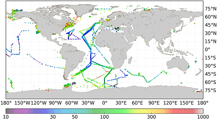
Figure 1. Geographic distribution of Particulate Organic Carbon (POC) measurements within the in situ database. The color scale represents the averaged POC concentration (mg m⁻³) over the top 10 m.

FIGURE 2

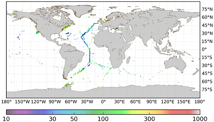
Figure 2. Locations of OC-CCI satellite data matchups and associated in situ concentrations of Particulate Organic Carbon (mg m⁻³).

FIGURE 3

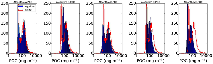
Figure 3. Histograms summarizing distribution of in situ POC data and associated satellite based estimates for (A) Algorithm A (Stramski et al., 2008, R_rs based), (B) Algorithm B (Stramski et al., 2008, b_bp based), (C) Algorithm C (by Loisel et al., 2002), (D) Algorithm D (by Gardner et al., 2006), (E) Algorithm E (by Kostadinov et al., 2016).

3.2. Algorithm Performance

The histogram of the in situ data frequency distribution is replicated to a degree by all the algorithms (Figure 3). The histogram of Algorithm A is very similar to that of the in situ data, with both histogram shapes and peak locations reproduced. Algorithm B tends to overestimate the POC values relative to in situ data at the lower end of POC concentrations, resulting in the first peak in the histogram being offset toward the right of the figure (i.e., toward higher POC concentrations). By contrast, Algorithm C underestimates POC slightly, at the lower end. The range of estimates provided by Algorithm D is narrower than that of the in situ data. Algorithm E also has a narrower range, and in general underestimates POC concentrations. Both algorithms D and E show significant shifts in both peaks of the distribution relative to those of the in situ data.

As could be expected from the histograms (Figure 3), there is generally a high correlation between the algorithm estimates and in situ measurements of POC, with r values between 0.75 and 0.82 for all algorithms tested (Figures 4A–E). It is of note that all algorithms show a small cloud of underestimated concentrations associated with high in situ POC. These points are from different data sources, and from different regions, and as such, outliers do not appear to be related to any systematic errors in the in situ measurements. Furthermore, not all of these substantial underestimates are associated with common data points across all the algorithms. It is important to note, however, that although we compare the satellite-derived POC with in situ POC over a very broad range, extending to very high values >1,000 mg m⁻³, the original formulations of the algorithms were not, in general, implemented with such high POC data.

FIGURE 4

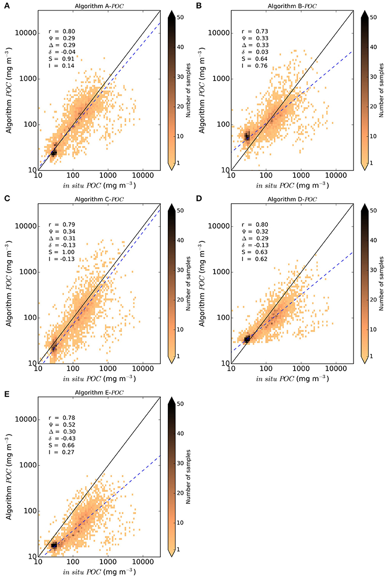
Figure 4. Scatter plots and statistics detailing performance of (A) Algorithm A by Stramski et al. (2008) (using R_rs), (B) Algorithm B by Stramski et al. (2008) (using b_bp), (C) Algorithm C by Loisel et al. (2002), (D) Algorithm D by Gardner et al. (2006), and (E) Algorithm E by Kostadinov et al. (2016). Statistical parameters are as follows: correlation coefficient (r), bias (δ), Root Mean Square Difference (Ψ), Center Patterned Root Mean Square Difference (Δ), slope (s), intercept (I). The solid line is the 1:1 line, and the dashed line is the line of best fit for the linear regression.

The scatter plots and uncertainty statistics for Algorithm A shown in Figure 4A and Table 1 suggest that this algorithm, on average, performs better than the other algorithms shown in Figures 4B–E. Algorithm A has the smallest bias, a linear fit that is closest to the 1:1 line, with a slope of 0.92 and a relatively small intercept value (the second smallest after Algorithm C), and also the highest (albeit slightly) correlation coefficient and the smallest values (albeit slightly) of the Root Mean Square Difference. The statistical parameters are consistently good for Algorithm A, though the results for Algorithm C also present some advantages. The performance of Algorithm C has a slope of 1 and intercept closest to zero, but has a slightly higher RMSD, CRMSD and bias compared with Algorithm A (Figure 4C). Algorithm B has relatively small bias, however other parameters are clearly inferior compared with Algorithm A (Figure 4B). Some statistical parameters associated with the performance of Algorithm D are significantly inferior compared with those associated with algorithms A and C, especially the slope and intercept of linear fit which indicate a large deviation of this fit from the 1:1 line (Figure 4D). As a result, low values of POC are overestimated, and high values underestimated, compared with the in situ data. The statistical performance for Algorithm E is poorest with significant negative bias and the best fit regression deviating greatly from the 1:1 line (Figure 4E). Performance statistics are summarized for all algorithms in the first section of Table 1. A statistical analysis was also conducted for the non-transformed data, and provided in the second section of Table 1.

TABLE 1

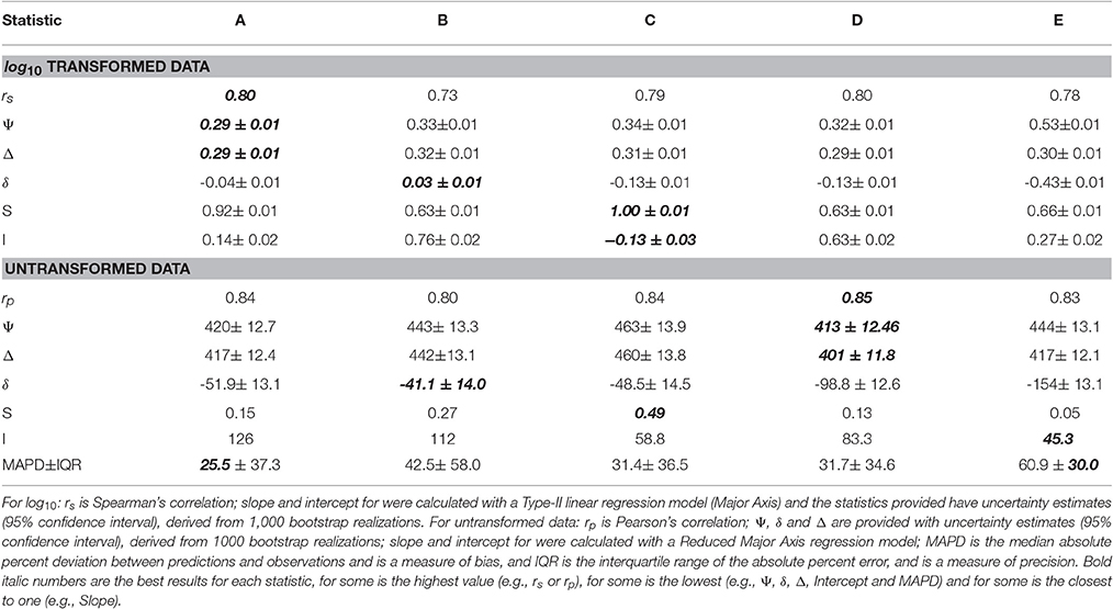
Table 1. Summary of statistics of the algorithm performances for log₁₀ and untransformed data.

3.3. Performance Per Water Class

To further understand algorithm performance, the matchups were separated by their optical water class. The total number of matchups per water class, and their distribution spatially, is shown in Figures 5, 6 respectively. The lower water classes are associated with oligotrophic regions, such as in the gyres, whilst the higher classes correspond to progressively more turbid shelf and coastal waters. Statistical performance of the algorithms across the different water classes is summarized in Figure 7.

FIGURE 5

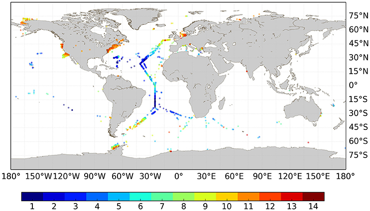
Figure 5. Locations and associated water class for each satellite-in situ matchup.

FIGURE 6

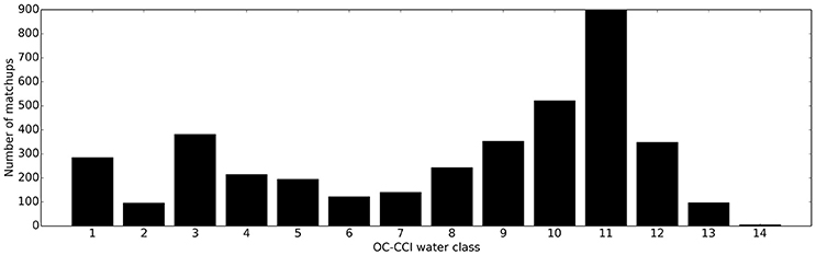
Figure 6. Histogram showing number of matchups associated with each OC-CCI water class.

FIGURE 7

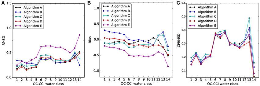
Figure 7. Calculated RMSD (A), Bias (B), and Center Patterned RMSD (C) for each algorithm per water class based on the matchup statistics.

Performing the statistical analysis across the different water classes reveals some similarities in performance across all algorithms, and some consistency with the overall performance (Figure 7). Algorithms A, C, and D show little differences between them in terms of RMSD across the water classes, with the exception of water class 14 (i.e., the most optically complex waters) (Figure 7A). The RMSD associated with Algorithm E follows the same broad pattern as algorithms A and D across the water classes, although its RMSD is substantially higher than those algorithms in all instances. Algorithm B shows slightly higher RMSD than the other algorithms in some of the more oligotrophic water classes (1–5), then largely follows the same patterns as algorithms A and D. The cloud of outlier points observed in the overall comparisons are associated with water classes 6, 7, and 8, where RMSD is relatively high for most of the algorithms. The estimates of bias for each of the water classes is consistent with the results from the global application e.g., Algorithm A shows very little bias, and this is consistent across water classes, whilst Algorithm E generally underestimates across all classes (Figure 7B). Algorithm C shows slight negative bias across most of the water classes, except 12 and 13, whilst algorithms D and B show slight (larger) positive bias in the more oligotrophic classes. Algorithm B shows large positive bias in water class 13, as with Algorithm C; however, both algorithms show negative bias in class 14. The center-pattern (or unbiased) RMSD in Figure 7C shows the largest uncertainties are associated with water classes 6, 7, and 8 whilst the largest differences in algorithm performance across the water classes are found in water classes 12, 13, and 14. The regional variability in algorithm performance, which can be associated with the optical water classes, is discussed further in Sections 3.4, 3.5, and 4.2 below.

3.4. Mapped Products

In addition to application to the matchups points, the POC algorithms can also be applied to global satellite data to compare algorithm performance at synoptic scales. POC concentrations were estimated by applying algorithms A-E to a sample set of OC-CCI monthly products from May 2005 (Figure 8). All algorithms produce the broad patterns that were observed in the in situ measurements and would be expected to be associated with POC, i.e., increased POC associated with regions of high [Chl] in upwelling zones, lower concentrations in the oligotrophic gyres, and higher concentrations in turbid shelf and coastal regions. However, there are some notable differences between the POC concentrations estimated by the different algorithms. Algorithm A and C perform similarly (Figures 8A,C). Algorithm B (Figure 8B) produces estimates that are generally higher relative to Algorithm A and C, particularly at low POC concentrations. Algorithm D (Figure 8D) underestimates at higher POC concentrations relative to all other algorithms, whilst at low concentrations its estimates are generally higher than algorithms A and C, and lower than algorithm B. In contrast, Algorithm E (Figure 8E) estimates lower POC concentrations relative to the other methods. A transect, extracted along from 20^o west, shows the regional differences in algorithm estimates for POC, and the associated OC-CCI [Chl] for reference (Figure 8F). Histograms of these products (not shown), show a similar range to the in situ data used for validation (≈ 10–1,000), though values greater than 1,000 mg m⁻³ are scarce in the satellite products (though higher values are more frequent with Algorithm C than with Algorithm A). Also, the pronounced bimodal frequency distribution of the in situ data is absent in the satellite products, which show a unimodal distribution. This difference between the frequency distribution of in situ data and satellite products could have had an impact on the comparative statistics presented here.

FIGURE 8

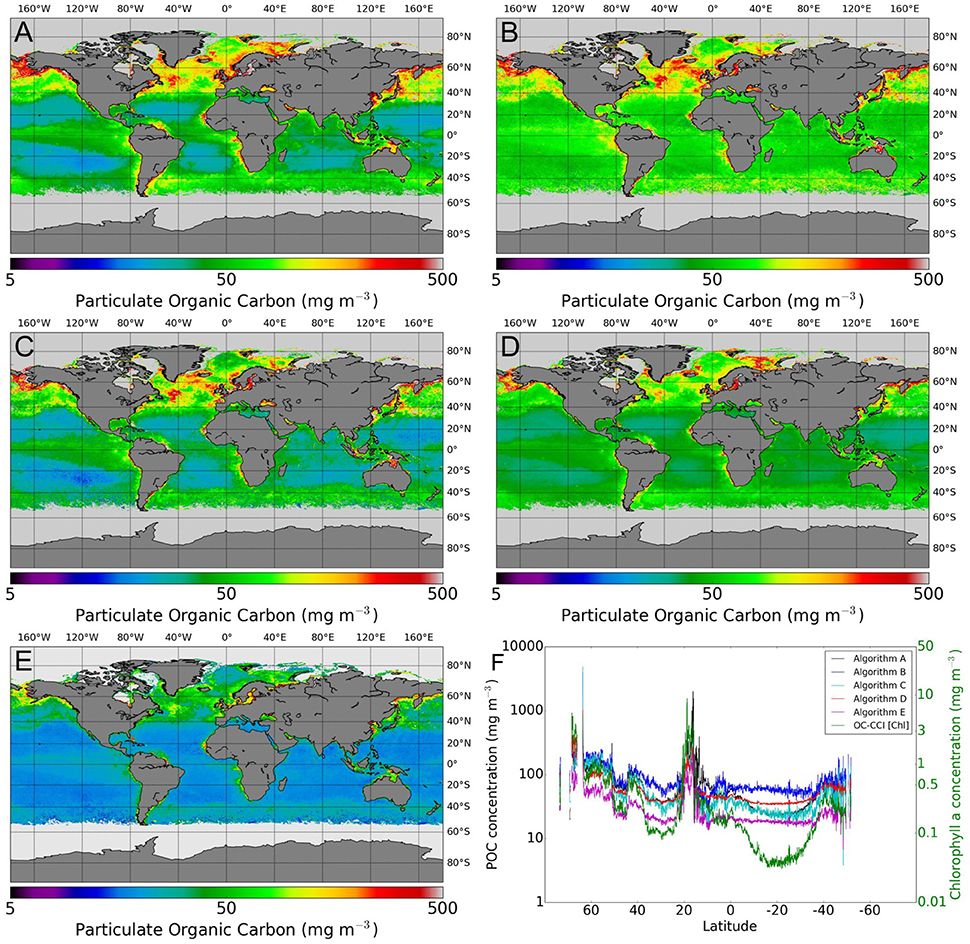
Figure 8. POC estimated using the five candidate algorithms applied to a monthly composite of OC-CCI data from May 2005 (A) Stramski et al. (2008) (R_rs), (B) Stramski et al. (2008) (b_bp), (C) Loisel et al. (2002), (D) Gardner et al. (2006), (E) Kostadinov et al. (2016), and (F) POC associated with an extracted transect through the Atlantic at 20^o W for each algorithm, and the associated [Chl] from the OC-CCI data.

3.5. Mapped Uncertainties

Each algorithm has uncertainties associated with its performance for each water class, calculated from the validation exercise. These values can be used to estimate uncertainties for pixels outside of direct matchup locations, using a weighted average based on the percent membership to each of the classes. This procedure was applied to the data in Figure 8 to calculate per pixel RMSD and bias. As could be expected from the performance of the algorithms across the substantial in situ data set, Algorithm A (R_rs based algorithm of Stramski et al., 2008) shows low RMSD and bias when uncertainties are calculated (Figures 9, 10). Algorithms B and particularly Algorithm C show higher RMSE, particularly in the gyre regions, consistent with the distribution of the matchup-based estimates in Figure 3. Algorithm D has low RMSD and bias in the oligotrophic gyres, but relatively higher values appear in the more productive (upwelling and coastal) areas. Algorithm E shows high RMSE throughout the image. Highest positive bias estimates are associated with algorithm B, relating to overestimation in the gyre regions (Figure 10B). Bias for Algorithm E (Figure 10E) shows negative bias globally, consistent with the general trend toward underestimation shown in Figures 4E, 8E.

FIGURE 9

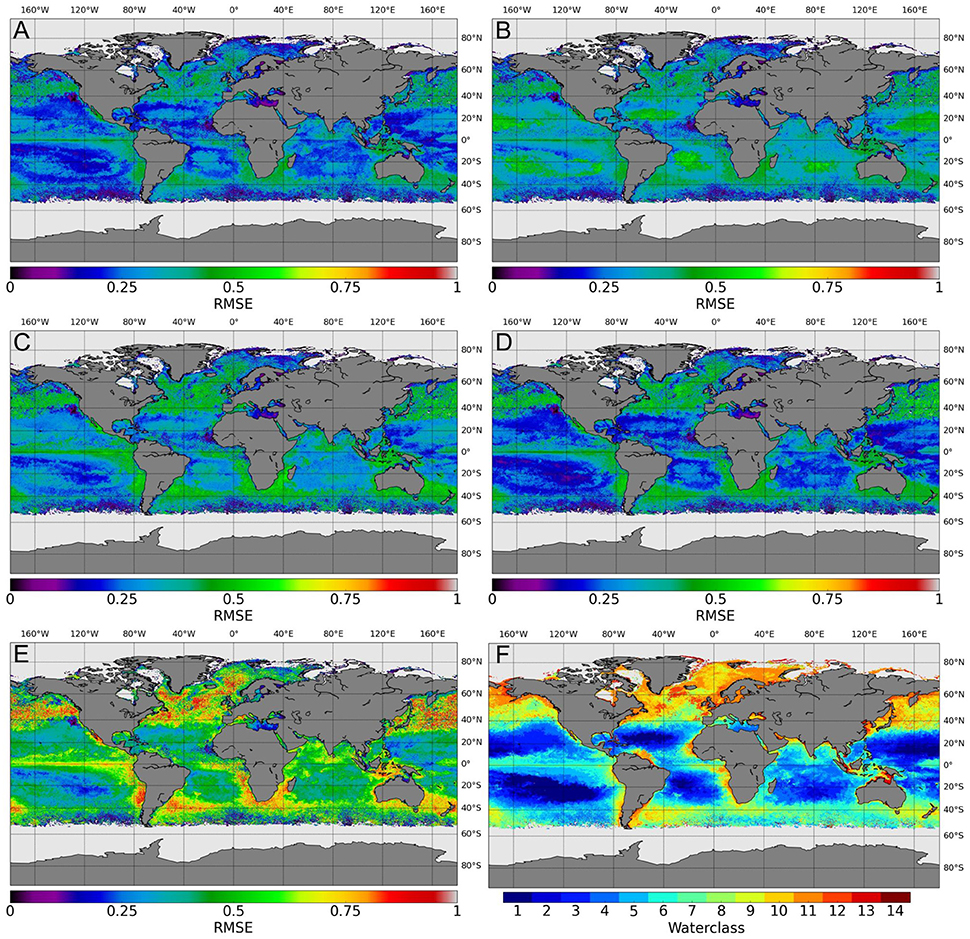
Figure 9. Root Mean Squared Difference calculated for POC as estimated using water-class specific performance of the the five candidate algorithms applied to monthly composite OC-CCI data from May 2005 (A) Stramski et al. (2008) (R_rs), (B) Stramski et al. (2008) (b_bp), (C) Loisel et al. (2002), (D) Gardner et al. (2006), (E) Kostadinov et al. (2016), and (F) the associated OC-CCI water classes.

FIGURE 10

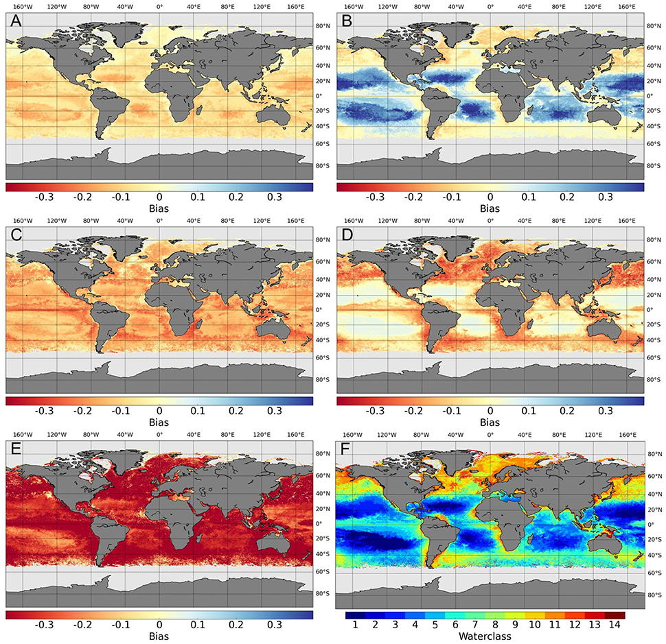
Figure 10. Bias as estimated using per water class performance of the five candidate algorithms applied to monthly composite OC-CCI data from May 2005 (A) Stramski et al. (2008) (R_rs), (B) Stramski et al. (2008) (b_bp), (C) Loisel et al. (2002), (D) Gardner et al. (2006), (E) Kostadinov et al. (2016), and (F) the associated OC-CCI water classes.

4. Discussion

4.1. Variability in Algorithm Performance As a Result of Input Satellite Data, Choice of Optical Models, and Regional Optical Properties

The strength of the relationships between bio-optical properties and POC concentration has been quantified in the original studies where the algorithms examined above were formulated, and in some cases, validated against satellite data. To the extent that some of the satellite data used in the original studies are included in the match-up dataset used here, the impact on the results is likely to be small because the size of the match-up data used here is much larger than that used in any of the previous studies. Furthermore, the comparisons presented here are based on a common satellite product suite (OC-CCI). However, further insights are gained from the bigger in situ data base assembled for this study, and from the climate-quality data set provided by OC-CCI.

Results from the OC-CCI based validation are generally consistent with the observations made by Stramski et al. (2008). The in situ data used by Stramski (Stramski et al., 2008) were limited to the south eastern Pacific and eastern Atlantic Oceans and covered a POC range of 12—270 mg m⁻³, whilst the range for the data used here cover a broader range (2.7–8,097 mg m⁻³). The waters sampled by Stramski et al. (2008) ranged from upwelling to oligotrophic, with significant contributions of mineral particle matter to the particle assemblage at some stations. Consistent with the results here, Stramski et al. (2008) found that empirical relationships between R_rs and POC performed better than two-step approaches where an inherent optical property (IOP) is derived from the R_rs and then related to the POC. They also indicated relatively better performance of the R_rs relationship over that derived from b_bp, highlighting the uncertainties in the derivation of b_bp as one source of error in estimation of POC from IOPs. Additionally, the relationships between POC and IOPs would be expected to vary as a result of the particle size distribution (PSD), the refractive index of particles, and the fractional POC concentrations within different particle types in the assemblage. For example, significant variations in the POC-specific backscattering coefficient has been reported for different water bodies of the Southern Ocean (see Figure 1 in Stramski et al., 1999). Whilst variability in the POC-specific backscattering introduces uncertainty in total POC estimates, a better understanding of the relationship between particle characteristics and IOPs has the potential to provide further insight into the composition of the POC pool, and therefore to improve POC algorithms. Hence, it is important to pursue this line of algorithm development, even if the current performance of these methods might not be as good as that of some more empirical approaches. The line of investigation that accounts for the contributions of different types of POC to their optical properties is already yielding fruit (Stramski et al., 2008).

The algorithm of Loisel et al. (2002) (Algorithm C) is also a two-step approach, drawing on the relationship between b_p and POC, via a relationship between b_bp and [Chl]. Though Loisel et al. (2002) did not directly validate their POC estimation from SeaWiFS data, they found a good match between retrieved b_bp and that measured in situ in a previous study (Loisel et al., 2001). Loisel et al. (2002) did indicate variability in the b_bp:[Chl] relationship, linked to changes in the particulate pool; they highlighted the variable influence of small particles consisting of dead cells, grazers, and minerals. Gardner et al. (2006) (Algorithm D) also uses a two-step approach, exploiting the relationship between the beam attenuation coefficient (c_p) and POC. This relationship was shown to be strong, when in situ POC was compared with transmissometer profiles. Although no fully-validated algorithm exists for routine derivation of c_p from satellite ocean color measurements, Gardner et al. (2006) showed in situ c_p was strongly correlated with [Chl] (r = 0.845–0.897) and K_d(490)) (r = 0.846-0.878) derived from SeaWIFS data over different oceanic regions.

Algorithm E, by Kostadinov et al. (2016), addresses some sources of variability between optical properties and POC, such as the influence of the particle size distribution, which was also identified as being important by Stramski et al. (2008). The method of Kostadinov et al. (2016) uses spectral values of b_bp to derive a PSD, which is then converted to POC (and phytoplankton carbon) using allometric relationships. The focus of the Kostadinov et al. (2016) paper was on phytoplankton carbon, computed as 1/3 of POC. Relationships between the phytoplankton carbon estimated from in situ PSD measurements and direct analytical determinations, showed r values between 0.5 and 0.714, depending on the limits of integration of the PSD, with wider limits resulting in the lower r. As discussed by Stramski et al. (2008), Kostadinov et al. (2016) also notes the impact of uncertainties in retrieved backscattering arising from both measurement and theory. In particular, assumptions of sphericity and homogeneity used in Mie theory are likely to be violated in real seawater particle assemblages, particularly for backscattering and in coastal and more productive areas (which are included in the database used here). For a more detailed discussion of the sphericity and homogeneity assumption, see Kostadinov et al. (2009) and refs. therein. Future work needs to focus on developing and more widely adopting bio-optical models that relax the Mie assumptions (e.g., Quirantes and Bernard, 2004, 2006; Clavano et al., 2007; Matthews and Bernard, 2013; Robertson Lain et al., 2017). Understanding of PSD variability, how it relates to backscattering, and how particle composition affects scattering over broad marine regions are required to develop further such detailed mechanistic approaches.

General sources of error associated with any ocean-color product include differences introduced by choice of sensor, sensor calibration, and the atmospheric correction procedure used to retrieve R_rs. In addition to these, a further consideration, particularly in the cases where algorithms use IOPs, is the methods used to derive the IOP product from the R_rs data. The OC-CCI processing uses the Quasi-Analytical Algorithm (QAA) of Lee et al. (2002) to calculate IOPs, including the b_bp values used in this study. The original study by Kostadinov et al. (2016) used the method of Loisel and Stramski (2000) to estimate b_bp. Stramski et al. (2008) also used different formulations to calculate b_bp from R_rs, finding a corrected version of QAA produced a better estimate of b_bp, and a strong relationship with POC (r = 0.933). The effect of the choice of method to derive b_bp on the POC estimates requires further consideration, which goes beyond the scope of this study, as this IOP is particularly poorly understood and validated (Lee et al., 2002). The differences in algorithm performance across the different water classes indicate that regional variability in performance of the different algorithms can be expected. This is confirmed in the mapped regional distribution of uncertainties (Figures 9, 10). These results suggest that algorithms either need to be selected carefully for applications in different regions, or that a selection of optimal algorithms may have to be blended for a global product (as done in Jackson et al., in press). This point is also raised in Stramski et al. (2008), where different formulations are provided for global application, and excluding upwelling data. Uncertainties in the underlying satellite data may also be responsible for a portion of this variability: for example, an IOP model may be more or less suitable to derive backscattering. It should also be noted that there can also be uncertainties in the in situ data and the validation process that can affect the assessment of uncertainties in algorithm performance. Ideally, multiple replicates will be taken to quantify uncertainties in the in situ measurement, and instruments will have a well-characterized calibration history, and be processed with community endorsed methodologies. For POC, the issue of blank correction was already highlighted in Section 2.1. Uncertainties resulting from variable methods used for the in situ data collated for this study may influence the results presented here, particularly at low POC concentrations. In terms of comparison to matchups, further uncertainties can be introduced by comparing values at different scales, i.e., point measurements may not represent the average over a pixel (in this case of 4 km in size). These uncertainties will limit the ultimate accuracy to which any satellite based product can be derived and validated. However, issues of spatial mismatch are beginning to be addressed with the use of underway systems (for example, Brewin et al., 2016).

Despite the difficulties highlighted above, the overall performance of the algorithms studied here is encouraging. Percentage error estimates based on the OC-CCI methodology show how well these algorithms can generate products suitable for the needs of the scientific community. For example, the percentage errors associated with the Stramski et al. (2008) R_rs algorithm applied to OC-CCI data in May 2005 (Figure 11), show that a majority of pixels fall within an error range that is widely accepted by the ocean color community for [Chl] (30%; GCOS, 2011).

FIGURE 11

Figure 11. Percentage error for POC as estimated using per water class performance of the Stramski et al. (2008) (R_rs) applied to monthly composite OC-CCI data from May 2005.

4.2. Variability in the Ratio of Particulate Organic Carbon to Chlorophyll-a

Further perspective on the performance of the different algorithms can be gained by considering the covariance between POC and [Chl]. The relationship between the in situ POC data and satellite [Chl] is shown in Figure 12A, where the color indicates the associated dominant optical water class. These data then forms the background for each of the subsequent panels of Figure 12, which show the relationship between the POC estimated by each algorithm, and the satellite [Chl]. Algorithm A shares a commonality in method with the algorithms used to derive satellite [Chl], in that the same reflectance ratios are used to derive POC, and [Chl] (at lower concentrations); hence it shows a very constrained relationship in this domain of the parameter space (Figure 12B). Other algorithms capture the scatter in the POC:[Chl] relationship to a greater or lesser degree, though offsets can be seen, associated with the behavior identified in the validation exercise, i.e., overestimation of POC relative to lower [Chl] in the case of Algorithm B (Figure 12C), and underestimation of the ratio at low [Chl] using POC from Algorithm C (Figure 12D—though it should also be noted that this algorithm is also dependent on [Chl] to derive POC). As with Algorithm A, Algorithm D shows a relatively constrained relationship between POC and [Chl]. Algorithm E produces similar variability between POC and [Chl] as seen in the in situ data, in terms of shape and scatter of the curve, but the bias of this algorithm toward lower estimates of satellite derived POC is clear (Figure 12D).

FIGURE 12

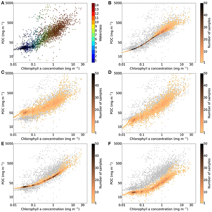
Figure 12. Covariance between POC and [Chl] extracted from the OC-CCI matchups with the in situ database for (A) in situ POC data, (B) POC estimated using Stramski et al. (2008) (R_rs), (C) POC estimated using Stramski et al. (2008) (b_bp), (D) POC estimated using Loisel et al. (2002), (E) POC estimated using Gardner et al. (2006), (F) POC estimated using Kostadinov et al. (2016).

The ratio of POC to [Chl] is important in the context of the discussion here for two reasons. Firstly, this ratio is important in the context of biogeochemical modeling, and the ecological and physiological processes that influence this ratio. Secondly, empirical relationships between POC and chlorophyll have been developed, which can be applied to satellite derived estimates of [Chl]. As mentioned above, these algorithms are typically similar to those employing blue:green reflectance ratios (e.g., Algorithm A from Stramski et al., 2008), and as such were not initially considered in the algorithm intercomparison here. Figure 13A shows a number of these empirical relationships, against a background of the same in situ POC and [Chl] data as shown in Figure 12. Figure 13B shows POC estimated using these [Chl]-based algorithms on OC-CCI [Chl] as a function of the blue-green R_rs reflectance ratio. The same reflectance ratio is employed by Stramski et al. (2008) to derive POC, and is also used in a number of empirical [Chl] algorithms. A linear regression of the in situ POC concentrations, against the satellite derived [Chl], results in an r² value of 0.70. Using the various relationships shown in Figure 13A to estimate POC based on the satellite [Chl] returns r² values between 0.63 and 0.69, lower than those returned for all the other algorithms assessed. The [Chl] based approaches show in Figure 13 produce RMSD values (between 0.27 and 0.47) and bias (between −0.03 and 0.117) in the same range as the other algorithms.

FIGURE 13

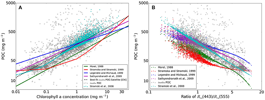
Figure 13. Summary of (A) POC to [Chl] relationships including the in situ POC data collated in this study and the extracted OC-CCI [Chl (gray dots)] and the relationships proposed by Morel (1988) (green line), Stramska and Stramski (2005) (red line), Legendre and Michaud (1999) (blue line), and Sathyendranath et al. (2009) (pink line), a best fit line for the in situ data vs. the OC-CCI chlorophyll (dashed line), and the estimated POC using Stramski et al. (2008) (cyan dots) are provided for context, (B) estimated POC from the previously listed approaches, plotted against the R_rs (443) to R_rs(555) to show relationship to this ratio commonly used in algorithms to derive [Chl].

Even though to first order Chl and POC are positively correlated in the global ocean, a residual scatter in the relationship remains (e.g., in satellite observations—Figure 12A, and in situ observations as well—e.g., Kostadinov et al., 2012). Ideally, a POC algorithm should be able to retrieve POC independently of [Chl] and capture the variable POC/[Chl] ratio correctly. Note that this ratio can vary due to both variability in the fraction of living phytoplankton carbon in the total POC pool, due to the physiology and photoacclimation of the phytoplankton component of POC (Geider, 1987; Geider et al., 1998; Behrenfeld et al., 2005), and species specific differences among phytoplankton themselves (Stramski, 1999). Therefore, independent knowledge of total POC, living phytoplankton carbon, and [Chl a] should be the goal of future bio-optical algorithm development.

4.3. Estimates of Total Pools of Carbon

The OC-CCI archive can be used to estimate total pools of POC in the mixed layer, taking into account interannual and regional variability, which is well captured by this merged dataset. Algorithms A-D were applied to the monthly OC-CCI version 2 data, and the values integrated over the mixed-layer depth (derived from MIMOC, Schmidtko et al., 2013), assuming homogeneity over the mixed layer. These were then averaged over all the months and for all the years of the OC-CCI version 2 (1998-2012) to provide estimates of the average standing pool of POC as follows: Algorithm A: 0.86 Pg C, Algorithm B: 1.3 Pg C, Algorithm C: 0.87 Pg C, Algorithm D: 0.77 Pg C. These are larger than the estimate of Gardner et al. (2006) and smaller than the estimate of Stramska (2009). Comparison of these estimates with those of phytoplankton carbon pools estimated in a parallel study (Martinez-Vicente et al., in review), indicates that phytoplankton carbon represents between 17 and 48% of the total POC pool. Whilst this ratio shows considerable variability, the often assumed value of 1/3 for phytoplankton carbon:POC falls within this range. High levels of variability in the phytoplankton carbon to POC ratio were also observed in situ by Graff et al. (2015). Satellite based estimates calculated by Kostadinov et al. (2016) (using a different set of mixed layer depth values) suggest a phytoplankton carbon standing stock of around 0.24 Pg C, implying a corresponding POC stock of around 0.72 Pg C when using the 1/3 assumption. Kostadinov et al. (2016) showed the estimated phytoplankton standing stock to be similar to estimates derived from the application of both the Stramski et al. (2008) b_bp based algorithm, combined again with a 1/3 assumption and the method of Behrenfeld et al. (2005) to SeaWIFS data, and to model estimates from the Coupled Model Intercomparison Project 5 (CMIP5). The estimate of phytoplankton carbon standing stock from Kostadinov et al. (2016) is similar to that estimated by other size class based approaches, such as that of Roy et al. (2017) which used size classes derived from absorption to estimate a total phytoplankton carbon stock of 0.26 Pg C. Though the global estimates of POC from the different approaches assessed here are quite similar to each other, the differences are more pronounced at smaller scales, as can be seen in Figure 8F.

5. Conclusions

A variety of POC algorithms were applied to matchup pixels extracted from the satellite OC-CCI ocean color data, and validated against in situ data. The database used here represents the largest collection of in situ POC data available, to the author's knowledge. The five algorithms showed strong predictive capacity for estimating POC, with Algorithm A (based on R_rs—Stramski et al., 2008) and C (based on Loisel et al., 2002) performing well across the broad range of the in situ dataset. Algorithms A and C performed consistently across different water types as defined in the OC-CCI data. From the water class based validation, errors can be estimated per pixel. For Algorithm A and C, the errors were mostly within the range requested by the user community. These results suggest a maturity in POC algorithms and their suitability for production of long term time series for climate related studies. However, several key points of development are highlighted from the inter comparison of the different algorithms and the various studies reviewed here. Greater knowledge of the composition of the particulate pool, and how it affects the IOPs of the oceans, may allow increased accuracy of POC algorithms (within the constraints of the sensitivities of current satellite ocean color radiometry), as well as providing further information on different types of particles, many of which play important roles in water quality and ocean biogeochemistry. To support this aim, further in situ data should be collected, including additional measurements to provide detail on phytoplankton community size structure, physiology, and photoacclimation. Further, it is recommended that future work seeks to use consistent methodology for blank correction of POC measurements, and clarify any trends in the low POC region which may be influenced by these uncertainties. Further understanding of the sources of variability between POC and optical parameters can then be incorporated in to future, semi-analytical algorithms. New understanding of these relationships may also inform future sensor development (e.g., hyperspectral sensors) and optical modeling techniques.

Author Contributions

HE: All the calculations, preparation of figures, lead on writing the manuscript. VM: Project manager for Pools of Carbon project; development of matchup processing and statistical analysis. RB: Provision of code for statistical analysis based on OC-CCI methodology. GD: Provision of in situ data, content on b_bp uncertainties and impact of particle sizing. AH: Perspectives on community requirements, particularly for ecosystem modeling. TJ: Provision of code for calculation of per optical water class uncertainties, based on the OC-CCI methodology. HK: Collation of the in situ database. TK: Algorithm provider, content on algorithm performance relating to particle size distributions. HL: Algorithm provider, content on regional variability in algorithm performance. SR: Input on statistical analysis and relative contributions of phytoplankton to the POC pool. RR: Collation of the in situ database. ST: Data contribution and guidance on POC data for the Southern Ocean. DS: Algorithm provider, content on history of POC algorithm development, and interpretation of comparative analysis of different algorithms. TP: Project leader, scientific advice. SS: Development of the concept and work plan, guidance of HEK, review and rewriting of various sections of manuscript. All authors reviewed and provided comments on the draft manuscript.

Funding

The POCO project is funded by the European Space Agency (ESA) under the program of Science Exploitation of Operational Missions (SEOM) following Contract: 4000113692/15/I-LG. This study is a contribution to the Ocean Color Climate Change Initiative of the European Space Agency, and to the activities of the National Center for Earth Observations (NCEO) of the Natural Environmental Research Council (NERC) of UK. This study is also a contribution to the international IMBER project and was supported by the UK Natural Environment Research Council National Capability funding to Plymouth Marine Laboratory and the National Oceanography Center, Southampton. AMT data were supported by the UK Natural Environment Research Council National Capability funding to Plymouth Marine Laboratory and the National Oceanography Center, Southampton. This is contribution number 309 of the AMT programme. TK was supported on NASA grant #NNX13AC92G and by the Division of Hydrologic Sciences, Desert Research Institute. The contribution of HL was funded by the CNES/TOSCA program in the frame of the COYOTE project.

Conflict of Interest Statement

The authors declare that the research was conducted in the absence of any commercial or financial relationships that could be construed as a potential conflict of interest.

Acknowledgments

The authors would like to thank Peter Regner for his support and management of the POCO project. We would like to thank Oliver Fisher for his contributions to the project during his student internship. The authors would like to thank the participants of the Color and Light in the ocean from Earth Observation (CLEO) workshop, for their valuable discussions on POC, which contributed substantially to refining the approaches presented in this work. The authors would also like to thank the two reviewers who provided detailed and constructive comments which substantially improved this manuscript.

References

Allison, D. B., Stramski, D., and Mitchell, B. G. (2010). Empirical ocean color algorithms for estimating particulate organic carbon in the Southern Ocean. J. Geophys. Res. 115, C10044. doi: 10.1029/2009JC006040

CrossRef Full Text | Google Scholar

Behrenfeld, M. J., Boss, E., Siegel, D. A., and Shea, D. M. (2005). Carbon-based ocean productivity and phytoplankton physiology from space. Glob. Biogeochem. Cycles 19:GB1006. doi: 10.1029/2004GB002299

CrossRef Full Text | Google Scholar

Bishop, J. (1999). Transmissometer measurement of poc. Deep Sea Res. I 46, 353–369. doi: 10.1016/S0967-0637(98)00069-7

CrossRef Full Text | Google Scholar

Bohren, C. F., and Huffman, D. (1983). Absorption and Scattering of Light by Small Particles. New York, NY: Wiley.

Google Scholar

Boss, E., and Pegau, W. S. (2001). Relationship of light scattering at an angle in the backward direction to the backscattering coefficient. Appl. Opt. 40, 5503–5507. doi: 10.1364/AO.40.005503

PubMed Abstract | CrossRef Full Text | Google Scholar

Boyd, P., and Newton, P. (1995). Evidence of the potential influence of planktonic community structure on the interannual variability of particulate organic carbon flux. Deep-Sea Res. I 42, 619–639. doi: 10.1016/0967-0637(95)00017-Z

CrossRef Full Text | Google Scholar

Brewin, R. J. W., Dall'Olmo, G., Pardo, S., van Dongen-Vogels, V., and Boss, E. S. (2016). Underway spectrophotometry along the Atlantic Meridional Transect reveals high performance in satellite chlorophyll retrievals. Remote Sens. Environ. 183, 82–97. doi: 10.1016/j.rse.2016.05.005

CrossRef Full Text | Google Scholar

Brewin, R. J. W., Sathyendranath, S., Müller, D., Brockmann, C., Deschamps, P.-Y., Devred, E., et al. (2015). The ocean colour climate change initiative: Iii. a round-robin comparison on in-water bio-optical algorithms. Remote Sens. Environ. 162, 271–294. doi: 10.1016/j.rse.2013.09.016

CrossRef Full Text | Google Scholar

Buiteveld, H., Hakvoort, J. H. M., and Donze, M. (1994). “Optical properties of pure water,” in Proc. SPIE, 2258, Ocean Optics XII, ed J. S. Jaffe (Bergen: International Society for Optics and Photonics), 174–185.

Google Scholar

Cetinić, I., Perry, M. J., Briggs, N. T., Kallin, E., D'Asaro, E. A., and Lee, C. M. (2012). Particulate organic carbon and inherent optical properties during 2008 North Atlantic Bloom Experiment. J. Geophys. Res. Oceans 117:C06028. doi: 10.1029/2011JC007771

CrossRef Full Text | Google Scholar

Cho, B. C., and Azam, F. (1990). Biogeochemical significance of bacterial biomass in the ocean's euphotic zone. Mar. Ecol. Prog. Series 63, 253–259. doi: 10.3354/meps063253

CrossRef Full Text | Google Scholar

Claustre, H., Morel, A., Babin, M., Cailliau, C., Marie, D., Marty, J. C., et al. (1999). Variability in particle attenuation and chlorophyll fluorescence in the tropical pacific: scales, patterns, and biogeochemical implications. J. Geophys. Res. Oceans 104, 3401–3422. doi: 10.1029/98JC01334

CrossRef Full Text | Google Scholar

Clavano, W. R., Boss, E., and Karp-Boss, L. (2007). Inherent optical properties of non-spherical marine-like particles - From theory to observation. Oceanogr. Mar. Biol. 45, 1–38. doi: 10.1201/9781420050943.ch1

CrossRef Full Text | Google Scholar

Dall'Olmo, G., Westberry, T., Behrenfeld, M. J., Boss, E., and Slade, W. (2009). Significant contribution of large particles to optical backscattering in the open ocean. Biogeosciences 6, 947–967. doi: 10.5194/bg-6-947-2009

CrossRef Full Text | Google Scholar

Ducklow, H., Steinberg, D. K., and Buesseler, K. O. (2001). Upper ocean carbon export and the biological pump. Oceanography 14, 50–58. doi: 10.5670/oceanog.2001.06

CrossRef Full Text | Google Scholar

Efron, B. (1979). Bootstrap methods: another look at the jackknife. Ann. Stat. 7, 1–26. doi: 10.1214/aos/1176344552

CrossRef Full Text

Efron, B., and Tibshirani, R. J. (1993). An Introduction to the Bootstrap. Boca Raton, FL: Chapman and Hall/CRC.

Google Scholar

Gardner, W., Mishonov, A., and Richardson, M. J. (2006). Global poc concentrations from in situ and satellite data. Deep Sea Res. II 53, 718–740. doi: 10.1016/j.dsr2.2006.01.029

CrossRef Full Text | Google Scholar

Gardner, W., Walsh, I., and Richardson, M. J. (1993). Biophysical forcing of particle production and distribution during a spring bloom in the north atlantic. Deep Sea Res. II 40, 171–195. doi: 10.1016/0967-0645(93)90012-C

CrossRef Full Text | Google Scholar

GCOS (2011). Systematic Observation Requirements from Satellite-Based Data Products for Climate 2011 Update. Supplemental Details to the Satellite-Based Component of the “Implementation Plan for the Global Observing System for Climate in Support of the UNFCCC. Technical report, No. 154, World Meteorological Organisation (WMO), Geneva 2, Switzerland.

Geider, R. J. (1987). Light and temperature dependence of the carbon to chlorophyll a ratio in microalgae and cyanobacteria: implications for physiology and growth of phytoplankton. New Phytol. 106, 1–34. doi: 10.1111/j.1469-8137.1987.tb04788.x

CrossRef Full Text | Google Scholar

Geider, R. J., Maclntyre, H. L., and Kana, T. M. (1998). A dynamic regulatory model of phytoplanktonic acclimation to light, nutrients, and temperature. Limnol. Oceanogr. 43, 679–694. doi: 10.4319/lo.1998.43.4.0679

CrossRef Full Text | Google Scholar

Graff, J. R., Milligan, A. J., and Behrenfeld, M. J. (2012). The measurement of phytoplankton biomass using flow-cytometric sorting and elemental analysis of carbon. Limnol. Oceanogr. Methods 10, 910–920. doi: 10.4319/lom.2012.10.910

CrossRef Full Text | Google Scholar

Graff, J. R., Westberry, T. K., Milligan, A. J., Brown, M. B., Dall'Olmo, G., Dongen-Vogels, V. V., et al. (2015). Analytical phytoplankton carbon measurements spanning diverse ecosystems. Deep-Sea Res. Part I Oceanogr. Res. Pap. 102, 16–25. doi: 10.1016/j.dsr.2015.04.006

CrossRef Full Text | Google Scholar

Jackson, T., Sathyendranath, S., and Mélin, F. (in press). An improved optical classification scheme for the Ocean Colour Essential Climate Variable and its applications. Rem. Sens. Environ. doi: 10.1016/j.rse.2017.03.036

CrossRef Full Text | Google Scholar

Kitchen, J. C., and Zaneveld, J. R. (1992). A three-layered sphere model of the optical properties of phytoplankton. Limnol. Oceanogr. 37:1680. doi: 10.4319/lo.1992.37.8.1680

CrossRef Full Text | Google Scholar

Kostadinov, T. S., Milutinović, S., Marinov, I., and Cabré, A. (2016). Carbon-based phytoplankton size classes retrieved via ocean color estimates of the particle size distribution. Ocean Sci. 12, 561–575. doi: 10.5194/os-12-561-2016

CrossRef Full Text | Google Scholar

Kostadinov, T. S., Siegel, D. A., and Maritorena, S. (2009). Retrieval of the particle size distribution from satellite ocean color observations. J. Geophys. Res. Oceans 114:C09015. doi: 10.1029/2009JC005303

CrossRef Full Text | Google Scholar

Kostadinov, T. S., Siegel, D. A., Maritorena, S., and Guillocheau, N. (2012). Optical assessment of particle size and composition in the santa barbara channel, california. Appl. Opt. 51, 3171–3189. doi: 10.1364/AO.51.003171

PubMed Abstract | CrossRef Full Text | Google Scholar

Lee, Z., Arnone, R., Hu, C., Werdell, P. J., and Lubac, B. (2010). Uncertainties of optical parameters and their propagations in an analytical ocean color inversion algorithm. Appl. Opt. 49, 369–381. doi: 10.1364/AO.49.000369

PubMed Abstract | CrossRef Full Text | Google Scholar

Lee, Z., Carder, K. L., and Arnone, R. (2002). Deriving inherent optical properties from water color: a multiband quasi-analytical algorithm for optically deep waters. Appl. Opt. 41, 5755–5772. doi: 10.1364/AO.41.005755

PubMed Abstract | CrossRef Full Text | Google Scholar

Lee, Z., Du, K., and Arnone, R. (2005). A model for the diffuse attenuation coefficient of downwelling irradiance. J. Geophys. Res. 110:C02016. doi: 10.1029/2004JC002275

CrossRef Full Text | Google Scholar

Legendre, L., and Michaud, J. (1999). Chlorophyll a to estimate the particulate organic carbon available as food to large zooplankton in the euphotic zone of oceans. J. Plankton Res. 21, 2067–2083. doi: 10.1093/plankt/21.11.2067

CrossRef Full Text | Google Scholar

Loisel, H., Nicolas, J. M., Deschamps, P. Y., and Frouin, R. (2002). Seasonal and inter-annual variability of particulate organic matter in the global ocean. Geophys. Res. Lett. 29, 491–494. doi: 10.1029/2002GL015948

CrossRef Full Text | Google Scholar

Loisel, H., and Stramski, D. (2000). Estimation of the inherent optical properties of natural waters from the irradiance attenuation coefficient and reflectance in the presence of Raman scattering. Appl. Opt. 39, 3001–3011. doi: 10.1364/AO.39.003001

PubMed Abstract | CrossRef Full Text | Google Scholar

Loisel, H., Stramski, D., Mitchell, B. G., Fell, F., Fournier-Sicre, V., Lemasle, B., et al. (2001). Comparison of the ocean inherent optical properties obtained from measurements and inverse modeling. Appl. Opt. 40, 2384–2397. doi: 10.1364/AO.40.002384

PubMed Abstract | CrossRef Full Text | Google Scholar

Maffione, R. A., and Dana, D. R. (1997). Instruments and methods for measuring the backward-scattering coefficient of ocean waters. Appl. Opt. 36, 6057–6067. doi: 10.1364/AO.36.006057

PubMed Abstract | CrossRef Full Text | Google Scholar

Maritorena, S., d'Andon, O. H. F., Mangin, A., and Siegel, D. A. (2010). Merged satellite ocean color data products using a bio-optical model: characteristics, benefits and issues. Remote Sens. Environ. 114, 1791–1804. doi: 10.1016/j.rse.2010.04.002

CrossRef Full Text | Google Scholar

Martiny, A. C., Vrugt, J. A., and Lomas, M. W. (2014). Concentrations and ratios of particulate organic carbon, nitrogen, and phosphorus in the global ocean. Sci. Data 1:140048. doi: 10.1038/sdata.2014.48

PubMed Abstract | CrossRef Full Text | Google Scholar

Matthews, M., and Bernard, S. (2013). Using a two-layered sphere model to investigate the impact of gas vacuoles on the inherent optical properties of M. aeruginosa. Biogeosciences 10, 10531–10579. doi: 10.5194/bgd-10-10531-2013

CrossRef Full Text | Google Scholar

Mel'nikov, I. A. (1976). Finely dispersed fraction of suspended organic matter in eastern Pacific ocean waters. Oceanology 15, 182–186.

Menden-Deuer, S., and Lessard, E. J. (2000). Carbon to volume relationships for dinoflagellates, diatoms, and other protist plankton. Limnol. Oceanogr. 45, 569–579. doi: 10.4319/lo.2000.45.3.0569

CrossRef Full Text | Google Scholar

Meyer, R. A. (1979). Light scattering from biological cells: dependence of backscatter radiation on membrane thickness and refractive index. Appl. Opt. 18, 585–588. doi: 10.1364/AO.18.000585

PubMed Abstract | CrossRef Full Text | Google Scholar

Moore, T. S., Campbell, J. W., and Dowell, M. D. (2009). A class-based approach to characterizing and mapping the uncertainty of the MODIS ocean chlorophyll product. Remote Sens. Environ. 113, 2424–2430. doi: 10.1016/j.rse.2009.07.016

CrossRef Full Text | Google Scholar

Morel, A. (1974). “Optical properties of pure water and pure seawater,” in Optical Aspects of Oceanography, eds N. G. Jerlov and N. E. Steemann (New York, NY: Academic Press), 1–24.

Google Scholar

Morel, A. (1988). Optical modeling of the upper ocean in relation to its biogenous matter content (Case I waters). J. Geophysi. Res. 93, 10749–10768. doi: 10.1029/JC093iC09p10749

CrossRef Full Text | Google Scholar

Mueller, J. L. (2000). “SeaWiFS algorithm for the diffuse attenuation coefficient, K (490), using water-leaving radiances at 490 and 555 nm,” in SeaWiFS Postlaunch Calibration and Validation Analyses, Part, eds S. B. Hooker and E. R. Firestone (Greenbelt, MD: NASA), 24–27.

Müller, D., Krasemann, H., Brewin, R. J. W., Brockmann, C., Deschamps, P.-Y., Doerffer, R., et al. (2015). The Ocean Colour Climate Change Initiative: I. A methodology for assessing atmospheric correction processors based on in situ measurements. Remote Sens. Environ. 162, 242–256. doi: 10.1016/j.rse.2013.11.026

CrossRef Full Text | Google Scholar

O'Reilly, J. E., Maritorena, S., Mitchell, B. G., Siegel, D. A., Carder, K. L., Garver, S. A., et al. (1998). Ocean color chlorophyll algorithms for SeaWiFS. J. Geophys. Res. Oceans 103, 24937–24953. doi: 10.1029/98JC02160

CrossRef Full Text | Google Scholar

Quirantes, A., and Bernard, S. (2004). Light scattering by marine algae: two-layer spherical and nonspherical models. J. Quant. Spectros. Radiat. Trans. 89, 311–321. doi: 10.1016/j.jqsrt.2004.05.031

CrossRef Full Text | Google Scholar

Quirantes, A., and Bernard, S. (2006). Light-scattering methods for modelling algal particles as a collection of coated and/or nonspherical scatterers. J. Quant. Spectrosc. Radiat. Trans. 100, 315–324. doi: 10.1016/j.jqsrt.2005.11.048

PubMed Abstract | CrossRef Full Text | Google Scholar

Robertson Lain, L., Bernard, S., and Matthews, M. W. (2017). Understanding the contribution of phytoplankton phase functions to uncertainties in the water colour signal. Opt. Express 25, A151–A165. doi: 10.1364/OE.25.00A151

CrossRef Full Text | Google Scholar

Roy, S., Sathyendranath, S., and Platt, T. (2017). Size-partitioned phytoplankton carbon and carbon-to-chlorophyll ratio from ocean colour by an absorption-based bio-optical algorithm. Remote Sens. Environ. 194, 177–189. doi: 10.1016/j.rse.2017.02.015

CrossRef Full Text | Google Scholar

Sathyendranath, S., Brewin, R. J. W., Jackson, T., Mélin, F., and Platt, T. (in press). Ocean-colour products for climate-change studies: what are their ideal characteristics? Remote Sens. Environ. doi: 10.1016/j.rse.2017.04.017

CrossRef Full Text | Google Scholar

Sathyendranath, S., Groom, S., Grant, M., Brewin, R. J. W., Thompson, A., Chuprin, A., et al. (2016). ESA Ocean Colour Climate Change Initiative (Ocean-Colour-cci): Version 2.0 Data. Centre for Environmental Data Analysis. doi: 10.5285/b0d6b9c5-14ba-499f-87c9-66416cd9a1dc

CrossRef Full Text

Sathyendranath, S., Stuart, V., Nair, A., Oka, K., Nakane, T., Bouman, H., et al. (2009). Carbon-to-chlorophyll ratio and growth rate of phytoplankton in the sea. Mar. Ecol. Prog. Series 383, 73–84. doi: 10.3354/meps07998

CrossRef Full Text | Google Scholar

Schmidtko, S., Johnson, G. C., and Lyman, J. M. (2013). MIMOC: a global monthly isopycnal upper-ocean climatology with mixed layers. J. Geophys. Res. Oceans 118, 1658–1672. doi: 10.1002/jgrc.20122

CrossRef Full Text | Google Scholar

Sharp, J. (1974). Improved analysis for “particulate” organic carbon and nitrogen from seawater. Limnol. Oceanogr. 19, 984–989. doi: 10.4319/lo.1974.19.6.0984

CrossRef Full Text | Google Scholar

Stramska, M. (2009). Particulate organic carbon in the global ocean derived from SeaWiFS ocean color. Deep-Sea Res. Part I Oceanogr. Res. Pap. 56, 1459–1470. doi: 10.1016/j.dsr.2009.04.009

CrossRef Full Text | Google Scholar

Stramska, M., and Stramski, D. (2005). Variability of particulate organic carbon concentration in the north polar Atlantic based on ocean color observations with Sea-viewing Wide Field-of-view Sensor (SeaWiFS). J. Geophys. Res. 110:C10018. doi: 10.1029/2004JC002762

CrossRef Full Text | Google Scholar

Stramski, D. (1999). Refractive index of planktonic cells as a measure of cellular carbon and chlorophyll a content. Deep-Sea Res Part I-Oceanogra. Res. Pap. 46, 335–351. doi: 10.1016/S0967-0637(98)00065-X

CrossRef Full Text | Google Scholar

Stramski, D., and Kiefer, D. A. (1991). Light-scattering by microorganisms in the open ocean. Prog. Oceanogr. 28, 343–383. doi: 10.1016/0079-6611(91)90032-H

CrossRef Full Text | Google Scholar

Stramski, D., Reynolds, R. A., Babin, M., Kaczmarek, S., Lewis, M. R., Rottgers, R., et al. (2008). Relationships between the surface concentration of particulate organic carbon and optical properties in the eastern south pacific and eastern atlantic oceans. Biogeosciences 5, 171–201. doi: 10.5194/bg-5-171-2008

CrossRef Full Text | Google Scholar

Stramski, D., Reynolds, R. A., Kahru, M., and Mitchell, B. G. (1999). Estimation of particulate organic carbon in the ocean from satellite remote sensing. Science 285, 239–242. doi: 10.1126/science.285.5425.239

PubMed Abstract | CrossRef Full Text | Google Scholar

Thomalla, S. J., Ogunkoya, A. G., Vichi, M., and Swart, S. (2017). Using optical sensors on gliders to estimate phytoplankton carbon concentrations and chlorophyll-to-carbon ratios in the Southern Ocean. Front. Mar. Sci. 4, 133–119. doi: 10.3389/fmars.2017.00034

CrossRef Full Text | Google Scholar

Twardowski, M. S., Boss, E., and Macdonald, J. B. (2001). A model for estimating bulk refractive index from the optical backscattering ratio and the implications for understanding particle composition in case I and case II waters. J. Geophys. Res. 106, 14129–14142. doi: 10.1029/2000JC000404

CrossRef Full Text | Google Scholar

Volk, T., and Hoffert, M. I. (1985). Ocean carbon pumps: analysis of relative strengths and efficiencies in ocean-driven atmospheric CO₂ changes. Carbon Cycle Atmosph. CO₂ Nat. Variat. Archean Present 32, 99–110.

Google Scholar

Werdell, P. J., and Bailey, S. W. (2005). An improved in situ bio-optical data set for ocean color algorithm development and satellite data product validation. Remote Sens. Environ. 98, 122–140. doi: 10.1016/j.rse.2005.07.001

CrossRef Full Text | Google Scholar

Zhang, X., Hu, L., and He, M.-X. (2009). Scattering by pure seawater: effect of salinity. Opt. Exp. 17, 5698–5710. doi: 10.1364/OE.17.005698

PubMed Abstract | CrossRef Full Text | Google Scholar