Can Empirical Algorithms Successfully Estimate Aragonite Saturation State in the Subpolar North Atlantic?

Introduction

Complex horizontal and vertical circulation in the subpolar North Atlantic has the potential to influence global ocean circulation and climate patterns. Deep water formation coupled with strong winds, and high rates of primary production in spring and summer result in this region of the subpolar North Atlantic acting as a strong sink for atmospheric carbon dioxide (DeGrandpre et al., 2006; Pérez et al., 2008). Over the past two decades an increase in surface water pCO₂ at a rate greater than that of the atmosphere has been observed in the Irminger Sea (Olafsson et al., 2009; Bates et al., 2014). In response to this increasing pCO₂, the surface water pH and the aragonite saturation states (Ω_Ar) show a decreasing trend (Vazquez-Rodriguez et al., 2012; García-Ibáñez et al., 2016). Pérez (2016), using the RCP8.5 scenario of the IPCC (2013), predicted that aragonite undersaturation (Ω_Ar < 1) in the Irminger basin would likely occur between 2050 and 2065, at atmospheric CO₂ levels between 510 and 640 ppm.

Most of the historical measurements of inorganic carbon (García-Ibáñez et al., 2016; Olsen et al., 2016) in the Irminger and Labrador basins have occurred on a few repeated transects over time, or at specific locations (Olafsson et al., 2009; Azetsu-Scott et al., 2010). The subpolar North Atlantic remains undersampled with respect to its scales of variability (Fröb et al., accepted), but novel sensor packages now being deployed on autonomous platforms (e.g., profiling floats, gliders, moorings) have the potential to dramatically increase observational coverage in time and space. Unfortunately, most of these platforms do not directly provide the set of two inorganic carbon measurements commonly used to derive Ω_Ar. This argues for a need to develop regional predictive algorithms to determine estimates of key water chemistry variables, such as Ω_Ar, from information contained in the measurements of commonly observed oceanic non-carbonate variables such as temperature (T), salinity (S), pressure (P), oxygen (O₂), and nutrients and/or variables that can be measured by autonomous sensors.

Previous studies have used multiple linear regression models (MLR) to estimate inorganic carbon variables from hydrographic measurements (Juranek et al., 2009, 2011; Kim et al., 2010; Alin et al., 2012; Bostock et al., 2013; Williams et al., 2016; Carter et al., 2017). These were applied to different data sets (hydrographic surveys, time-series, profiling floats, climatology) in order to reconstruct estimates of the natural variability of carbon variables. Juranek et al. (2009, 2011) used hydrographic surveys of T and O₂ to estimate Ω_Ar off the Oregon coast, and Argo profiling float T and O₂ profiles to estimate pH and Ω_Ar in the northeastern subarctic Pacific Ocean. Alin et al. (2012) reconstructed pH, carbonate saturation states, carbonate ion concentration, total dissolved inorganic carbon (TCO₂), and total alkalinity (TAlk) in the California Current System from T, O₂, S, and density. Williams et al. (2016) estimated pH in the Pacific sector of Southern Ocean from T, S, O₂, P, and nitrate (${\text{NO}}_3^{-}$). Furthermore, Bostock et al. (2013) used T, S, and O₂ to estimate TAlk and TCO₂ in the intermediate and deep waters of the Southern Hemisphere, while Kim et al. (2010) used T, P, and O₂ to estimate Ω_Ar in the Sea of Japan.

All these studies demonstrated that Ω_Ar can be robustly determined from measurements of commonly observed and/or non-carbonate oceanic variables and that MLR models provide a valuable tool for reconstructing Ω_Ar where direct observations of carbonate variables are not available. It is, however, expected that relationships between Ω_Ar and other variables will vary among different parts of the ocean suggesting a need for development of regional models. To our knowledge, such regional models have not been developed in the subpolar North Atlantic. While clearly not replacing direct measurements of inorganic carbon variables, these approaches produce estimates of Ω_Ar, including calculations of error, which can greatly expand the information in both space (e.g., in undersampled areas), and in time (e.g., during the wintertime where almost no inorganic carbon measurements are available). This will allow for better detection and attribution of ocean acidification (OA) related processes to anthropogenic CO₂ and identification of potential OA “hot spots,” while also improving the understanding of complex patterns and relationships between physical and chemical changes (e.g., during deep water convection, extreme wind events or fresh water input, and eddy activity) and the marine communities affected by OA. Regionally tuned empirical algorithms can also provide guidance for optimal placement (horizontal and depth) of additional autonomous platforms in the subpolar North Atlantic that augment current and planned ship surveys [e.g., Observatoire de la variabilité interannuelle et décennale en Atlantique Nord (OVIDE), AR7W, RedFish] and existing time-series [e.g., K1 mooring, Central Irminger Sea mooring (CIS), Overturning in the Subpolar North Atlantic Program (OSNAP)].

Quantifying predictive skill is key to assessing the effectiveness of any empirical algorithm. This includes the goodness of fit for the regressions of Ω_Ar on oceanographic variables and skill assessment metrics (Stow et al., 2009). These can help guide improvements in model structure, as well as aid in recognizing model limitations. Another important aspect of predictive skill is an empirical algorithm's ability to successfully predict “out of sample” (i.e., validation of the algorithm on an independent data not used in building the original regression model). This is particularly important when models are used as tools to support decision-making. While common in the statistical literature, such independent validation has not been adequately addressed by most of the previous studies in oceanography.

The goal of this study is to investigate the predictive skill of commonly observed non-carbonate and autonomous sensor oceanographic variables [T, S, P, O₂, ${\text{NO}}_3^{-}$, phosphate (${\text{PO}}_4^{3-}$), and silicate (Si(OH)₄), pH] in determining a key water chemistry variable (Ω_Ar) in the subpolar North Atlantic. This region is of high oceanographic interest due to its role in Atlantic Meridional Overturning (Jackson et al., 2016) and a major carbon dioxide sink (Sabine et al., 2004). The rationale for this work is to assess the potential for autonomous sensors and biogeochemical models to monitor Ω_Ar in undersampled regions of the ocean and to provide information to the research community for cost and benefit analysis to support decisions on selection of optimal sets of shipboard measurements and set of sensors for outfitting autonomous platforms. Regional algorithms are necessary as the empirical relationships between Ω_Ar and oceanographic variables would be expected to vary over broad domains with a wide range of oceanographic conditions (e.g., such as the whole North Atlantic). The specific objectives are to (1) develop regional empirical algorithms for the subpolar North Atlantic to determine Ω_Ar using existing data from GLODAPv2, which has not been done before; and (2) validate the algorithms against independent shipboard data (from the OVIDE2012 cruise) to assess its performance and to improve best practices in skill assessment methodology. As an illustration of how the algorithms trained with GLODAPv2 data can be applied to a set of commonly measured non-carbon variables we use the derived empirical algorithm with a time series data from Irminger Sea site, and from a mooring (Station K1 in the Labrador Sea), and estimate for the first time the variability of Ω_Ar over a full seasonal cycle.

Data

GLODAPv2 Data

Observations of oceanographic non-carbonate variables [T (°C), S, P (dbar), O₂ (μmol kg⁻¹), ${\text{NO}}_3^{-}$ (μmol kg⁻¹), ${\text{PO}}_4^{3-}$ (μmol kg⁻¹), Si(OH)₄ (μmol kg⁻¹)] and inorganic carbonate variables [TAlk (μmol kg⁻¹), pH (at in situ T and P), and Ω_Ar] were extracted from Global Ocean Data Analysis Project version 2 (GLODAPv2; Olsen et al., 2016). The input for our analysis are the vertically interpolated, horizontally bin averaged bottle data extracted from the mapped GLODAPv2 product (Lauvset et al., 2016). Each of these bin-averaged data points comes with an associated standard deviation, as well as the number of data in the bin. For further details on this data product the reader is referred to Lauvset et al. (2016) and the published metadata (available here: https://www.nodc.noaa.gov/archive/arc0107/0162565/1.1/data/0-data/mapped/). Note that in order to eliminate biases due to variable spatial and temporal resolution of the bottle data and an anthropogenically-driven trend, both the pH and Ω_Ar data were normalized to year 2002 before binning and averaging. The GLODAPv2 normalization was done by using anthropogenic carbon calculated with the transit time distribution (TTD) method (Hall et al., 2002; Waugh et al., 2006) to correct TCO₂ to year 2002. Ω_Ar was then calculated from the normalized TCO₂. The method is thoroughly described in Lauvset et al. (2016). The bin-averaged data were also used as the basis for the 1° latitude and longitude spatial statistical mapping by Lauvset et al. (2016), but we note that this global mapped product had large spatial scales incompatible with our limited regional focus.

Ω_Ar (at in situ T and P) in GLODAPv2 was calculated from the TCO₂ (normalized to year 2002 to remove anthropogenic influence) and TAlk. pH was calculated from the TCO₂ (normalized to year 2002 to remove anthropogenic influence) and TAlk at both in situ T and P, and at constant T (25°C) and P (0 dbar). All calculations for the carbonate system in GLODAPv2 were performed using the MATLAB version (van Heuven et al., 2009) of CO₂SYS (Lewis and Wallace, 1998) using T, S, P, ${\text{PO}}_4^{3-}$, and Si(OH)₄, the dissociation constants of Lueker et al. (2000) for carbonate, Dickson (1990) for sulfate, and the total borate–salinity relationship of Uppström (1974). The uncertainly in calculated Ω_Ar was about 0.05. For further details, see Olsen et al. (2016).

The geographical domain of our study was adapted from the southwestern portion of the Longhurst ARCT biogeochemical province (Longhurst, 1995; Figure 1-black line), and designed to reflect the approximate boundaries of the Irminger and most of the Labrador Sea. For each variable approximately 1630 data points in this domain were extracted from GLODAPv2 and used to develop empirical algorithms using a multiple linear regression (MLR) model (see section Methods). Note that the GLODAPv2 data (Figure 1-blue dots) has a well-recognized seasonal bias as this region of the subpolar North Atlantic is almost exclusively sampled in May–August (boreal summer). The bin-averaged data used here are thus representative of the summer season.

FIGURE 1

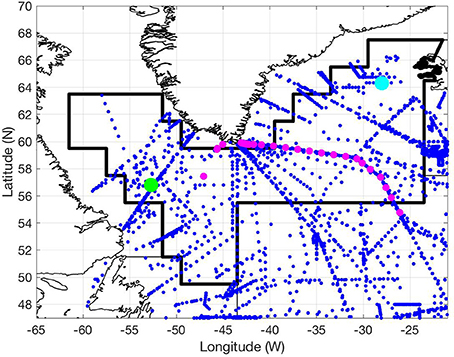
Figure 1. Map of the northern North Atlantic, showing GLODAPv2 bottle data locations (blue dots) with OVIDE2012 cruise stations (pink dots) and K1 mooring location (green dot) and Irminger Sea site (light blue dot). Black line represents the southwestern portion of Longhurst Atlantic-Arctic (ARCT) province, which is the study domain.

Shipboard Measurements

To validate the empirical algorithms derived from the regression analysis of the GLODAPv2 data [see section Multiple Linear Regression (MLR) Algorithms (Training)], we used Conductivity-Temperature-Depth (CTD) profiles and water samples for nutrients [${\text{NO}}_3^{-}$ (μmol kg⁻¹), ${\text{PO}}_4^{3-}$ (μmol kg⁻¹), and Si(OH)₄ (μmol kg⁻¹)], and inorganic carbon (TAlk and pH) from the OVIDE section across the Irminger Sea in summer 2012 (Figure 1-pink circles). These data were not included in GLODAPv2, because they were not submitted in time for inclusion in the database, and hence represent an independent data set. For the OVIDE2012 cruise, water samples were drawn at 108 stations from 0 to 5,400 m depth. TAlk was analyzed by single point titration (Mintrop et al., 2000; Pérez and Fraga, 2007) and calibrated with certified reference materials (CRMs) (Dickson et al., 2007) with overall accuracy of 4 μmol kg⁻¹. pH was determined at T = 25°C and P = 1 atm with a spectrophotometric method with uncertainty of 0.0055 pH units (Clayton and Byrne, 1993). Further details on the analysis of inorganic carbon is described in García-Ibáñez et al. (2016). As TCO₂ was not measured at OVIDE2012, Ω_Ar was calculated from TAlk and pH (total scale, at in situ T and P), and T, S, P, ${\text{PO}}_4^{3-}$, and Si(OH)₄ using the same MATLAB version of CO₂SYS (van Heuven et al., 2009) and constants (Uppström, 1974; Dickson, 1990; Lueker et al., 2000) as used in GLODAPv2. The estimated uncertainty in calculated Ω_Ar using a perturbation (Monte Carlo) method and uncertainties of 6 μmol kg⁻¹ for TAlk and 0.01 for pH, were between 0.020 and 0.056 (Perez, personal communication). Nutrient analyses were performed using a SKALAR segmented flow auto-analyser, and oxygen samples were analyzed by the Winkler method. Details of the analysis are given in the CATARINA Cruise report (https://cchdo.ucsd.edu/cruise/29AH20120622). Given that there is a non-negligible uncertainty associated with the calculation of Ω_Ar, and that the calculation from TAlk and pH yield slightly different answers compared to using the Talk and TCO₂ combination as in GLODAPv2, this adds further rationale for performing skill assessment using independent validation (i.e., while every effort is made to ensure consistency, independently collected data will always have its own unique features). We also note the observed decrease in pH [−0.025 pH decade⁻¹ in the Irminger Sea, Bates et al. (2014)] as a consequence of increase in TCO₂ since 2002 due to invasion of anthropogenic CO₂. For validation of the regression analysis we extracted the subset of OVIDE2012 data from 0 to 3,500 m at those stations and depths where the complete set of analysis variables was available (303 points for each variable).

Time Series

As an illustration of how the algorithms trained with GLODAPv2 data can be applied to a set of commonly measured non-carbon variables to predict seasonal variability of Ω_Ar in the surface waters, we used time series data of T, S, P, and O₂ at 10 and 100 m depth from two sites in subpolar North Atlantic (Figure 1): (1) Irminger Sea site (64.3°N, 28°W, Olafsson, 2016), and (2) the K1 mooring (56.5°N, 52.6°W) in Labrador Sea.

For Irminger Sea site, we used T, S, P, and O₂ data from 2010 to 2012, measured four times per year (February, May, August, November). We also used T, S, P, TCO₂, pCO₂, ${\text{PO}}_4^{3-}$, and Si(OH)₄ to compute Ω_Ar using CO₂SYS for comparison with estimated Ω_Ar. For the K1 mooring we have high frequency T, S, P, and O₂ data from August 2014 to March 2015. O₂ measurements from the K1 mooring were inter-calibrated when the mixed layer encompassed both sensors, and matched to a CTD profile taken prior to deployment. The details on measurements are described in Koelling et al. (2017). Observations of inorganic carbon variables at K1 mooring location during our time-series observations were not available.

Methods

The saturation state (Ω_Ar) for the aragonite is calculated as:

$\begin{array}{ll}{\Omega }_{\text{Ar}}=\left[{\text{Ca}}^{2+}\right]\left[{\text{CO}}_3^{2-}\right]/\text{K}{\text{'}}_{\text{sp}}& (1)\end{array}$

where [Ca²⁺] is concentration of calcium ions, [${\text{CO}}_3^{2-}$] is concentration of carbonate ions and K'_sp is the stoichiometric solubility product for aragonite. [Ca²⁺] changes in seawater are related to S, but they are small, therefore Ω_Ar is largely determined by changes in [${\text{CO}}_3^{2-}$] and K'_sp. [${\text{CO}}_3^{2-}$] can be calculated from TCO₂ and TAlk, where TCO₂ varies (non-linear) with physical conditions and biological activity (Barbero et al., 2011) and TAlk with T and S (linear) (Lee et al., 2006). K'_sp, is a function (non-linear) of T, S, and P. In the open ocean, we expect (1) TCO₂ to increase with higher uptake of nutrients and decrease with production of O₂, (2) TAlk to increase with T and S, and (3) K'_sp to decrease with T and increase with P and S. We thus anticipate that Ω_Ar will also vary with all these variables (most likely non-linear); generally to increase with T, O₂, and pH, and decrease with P and nutrients. The relationship with S is harder to predict, as well as whether the relationships of these variables with non-conservative quantity, such as Ω_Ar could be predicted with linear function.

Multiple Linear Regression (MLR) Algorithms (training)

MLR was used to develop a predictive relationship for Ω_Ar in the subpolar North Atlantic in 0–3,500 m, which is referred to as the “training” of the algorithm. MLR used GLODAPv2 Ω_Ar as the response variable and a subset of the GLODAPv2 data [T, S, P, pH, TAlk, O₂, ${\text{NO}}_3^{-}$, ${\text{PO}}_4^{3-}$, and Si(OH)₄] as predictor variables, all of which are potentially readily measureable quantities. The regression equation for the full model, which includes both non-carbonate variables and the autonomous sensor variables is:

$\begin{array}{l}{\Omega }_{\text{Ar}}={\beta }_0+{\beta }_1\text{T}+{\beta }_2\text{S}+{\beta }_3\text{P}+{\beta }_4\text{pH}+{\beta }_5{\text{O}}_2+{\beta }_6{\text{NO}}_3^{-}\\ +{\beta }_7{\text{PO}}_4^{3-}+{\beta }_8\text{Si}{\left(\text{OH}\right)}_4+\text{e}& (2)\end{array}$

where β_i are the regression coefficients (with β₀ representing the intercept) and e is the error term. Note that we do not include TAlk in the full model of Equation (2), but instead also consider a separate model with those predictor variables that are used as inputs to CO₂SYS to calculate Ω_Ar [i.e., T, S, P, TAlk, pH, ${\text{PO}}_4^{3-}$, and Si(OH)₄]:

$\begin{array}{l}{\Omega }_{\text{Ar}}={\beta }_0+{\beta }_1\text{T}+{\beta }_2\text{S}+{\beta }_3\text{P}+{\beta }_4\text{pH}+{\beta }_5\text{TAlk}+{\beta }_6{\text{PO}}_4^{3-}\\ +{\beta }_7\text{Si}{\left(\text{OH}\right)}_4+\text{e}& (3)\end{array}$

To account for both the sampling density and data spread, all regressions were weighted by the inverse of standard error making the weighting proportional to the square root of the number of data points per bin. Note that in all cases considered here, regression output yield error estimates for the regression parameters, as well as confidence and prediction intervals for estimated Ω_Ar.

For reasons of parsimony and interpretability we have chosen only to consider the oceanographic predictor variables in their original forma and not to consider higher order regression models wherein the predictor variables are combined into products and nonlinear polynomial relations are used. Similarly, we have explicitly decided not to include latitude and longitude as predictor variables. The rationale is that the regional domain for analysis has been chosen so that relationships should be relatively homogenous within it, and also that spatial variations (as embodied in latitude and longitude as predictors) can be easily confounded with changes in the primary oceanographic variable.

Two regression model building strategies were undertaken to identify the best set of oceanographic variables useful in predicting Ω_Ar. These strategies broadly correspond to (i) unsupervised and (ii) supervised learning (e.g., see Hastie et al., 2009). We used two types of unsupervised model building approaches. The first of these is “all possible regressions.” This approach considers all possible subsets of the predictor variables and can identify the regression model that has the best fit for a given number of predictor variables (i.e., the best regression based on one predictor, two predictors, etc.), as well as allow for assessment of the tradeoff in including different subsets of the available predictor variables. The second unsupervised approach was an automated selection of a set of best predictor variables for Ω_Ar based on the statistical model building technique of stepwise regression (Montgomery et al., 2015). Here, we performed stepwise predictor variable selection based on information criteria wherein regression fit (as measured by the coefficient of determination, R²) is balanced against model complexity (the number of predictor variables). We used the Bayesian Information Criterion (BIC) (Box et al., 1994), since this provides for a relatively strong complexity penalty relative to other information criteria (Plancherel et al., 2013). Three established stepwise approaches were implemented: forward selection, backward elimination, and forward/backward combination. For details on these techniques, the interested reader is referred to Montgomery et al. (2015), or most textbooks on multiple regression.

This unsupervised approach, however, does not take into account which variables are easy to measure, or which might be readily available through existing instruments or monitoring programs. Hence, we also use a scenario based, or “supervised learning,” approach to predict Ω_Ar. Three cases are considered: Scenario 1 uses non-carbonate variables [T, S, P, ${\text{NO}}_3^{-}$, ${\text{PO}}_4^{3-}$, Si(OH)₄] only; Scenario 2 uses variables that can be measured by autonomous sensors (T, S, P, O₂, pH, ${\text{NO}}_3^{-}$); and Scenario 3, designed to see how well a regionally tuned MLR model can represent the carbonate system in terms of predicting Ω_Ar using the inputs to CO₂SYS [i.e., T, S, P, TAlk, pH, ${\text{PO}}_4^{3-}$, and Si(OH)₄], and here is named the “CO₂SYS model.” For the first two scenarios we examine subsets of predictors to identify key variables. This strategy provides useful information toward a cost-benefit analysis to inform decisions on prioritization of shipboard measurements and outfitting of autonomous platforms.

Validation

The empirical algorithms were evaluated in terms of their ability to predict “out of sample,” i.e., validation based on an independent data set that was not used in training the regression model. Here an independent data set from the OVIDE2012 cruise (Figure 1) was used for validation. Specifically, the derived algorithms were applied to (subsets) of the predictor variables (Table 3) measured on the OVIDE2012 cruise. Predicted Ω_Ar from algorithms trained with GLODAPv2 climatological data were compared to “observed” Ω_Ar as calculated from carbon parameters (pH and TAlk) measured on the OVIDE2012 cruise. The quantitative metrics used to assess validation performance followed Stow et al. (2009), and a detailed interpretation is given there. Metrics included: correlation (r), root mean squared error (RMSE), the reliability index (RI), the average error (AE), the average absolute error (AAE), and the modeling efficiency (MEF). We have adopted the following quantification for MEF thresholds: MEF < 0.2 (poor), MEF 0.2–0.5 (good), MEF 0.5–0.65 (very good), and MEF > 0.65 (excellent; Allen et al., 2007; Nondal et al., 2009). These metrics, taken together, act to assess the bias and variability associated with applying the empirical algorithms to independent data.

Note that a few stations from the OVIDE2012 data set fall outside of our modified Longhurst ARCT biogeochemical province boundary (Figure 1). Specifically, stations closer to Greenland where a lower Ω_Ar could be expected due to higher fresh water input.

Results and Discussion

Depth Profiles of Variables

Depth profiles from 0 to 3,500 m from the GLODAPv2 data for all variables over the study domain, are presented in Figure 2 (blue dots). All variables show the highest variability in the upper 0–100 m, the approximate depth of the euphotic zone. This is the depth layer where photosynthesis, which acts to remove nutrients and TCO₂ and add O₂, is taking place. Consequently, there is a sharp decrease in ${\text{NO}}_3^{-}$, and ${\text{PO}}_4^{3-}$ and Si(OH)₄, and increase in O₂, pH, and Ω_Ar which reflects the seasonal bias in the GLODAPv2 data. In addition, the surface part of the euphotic zone (the approximate depth of 0–30 m) is also affected by local heating/cooling, freshwater inputs, and by air-sea exchange of CO₂ and O₂. During the boreal summer, when most GLODAPv2 data is collected, the subpolar North Atlantic Sea exhibits warming and increased fresh water input due to ice melt resulting in slightly higher T and lower S in this surface part of the euphotic zone in comparison to the layer below (30–100 m). In addition, nutrients concentrations are lower and pH higher at the surface layer due to strong biological uptake.

FIGURE 2

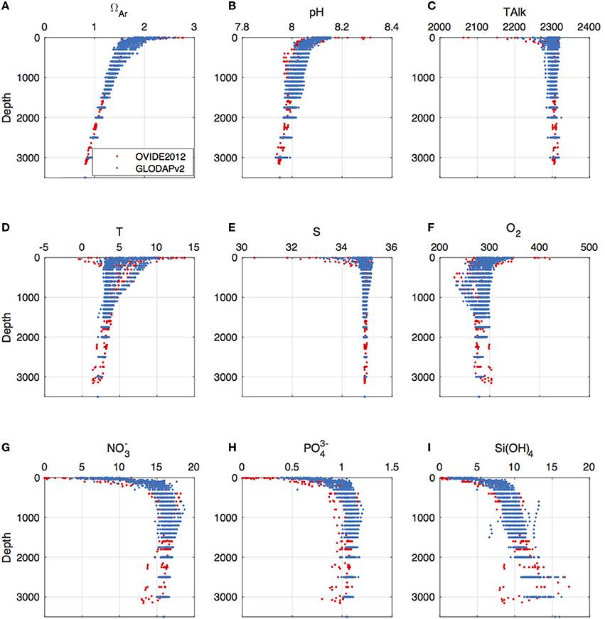
Figure 2. Depth profiles of (A) Ω_Ar, (B) pH (in situ), (C) TAlk (mol kg⁻¹), (D) T (oC), (E) S, (F) O₂ (mol kg⁻¹), (G) ${\text{NO}}_3^{-}$ (mol kg⁻¹), (H) ${\text{PO}}_4^{3-}$ (mol kg⁻¹), and (I) Si(OH)₄ (mol kg⁻¹) from GLODAPv2 data (blue) and OVIDE2012 cruise (red).

Below the euphotic zone (>100 m), where photosynthesis is not present, respiration and remineralization of nutrients and organic matter dominates. These processes lead to a gradual increase of ${\text{NO}}_3^{-}$, ${\text{PO}}_4^{3-}$, and Si(OH)₄, and lower O₂, pH and Ω_Ar. T decreases in this depth layer, but S and TAlk stay nearly constant. Below 1,000 m, T, pH, and Ω_Ar continue to decrease down to 3,500 m, while S, TAlk, O₂, ${\text{NO}}_3^{-}$, and ${\text{PO}}_4^{3-}$ stay nearly constant. Si(OH)₄ is the only variable that increases in deep layers due mainly to the deep water masses containing a higher fraction of water from the Arctic Sea (Ragueneau et al., 2001). There is also a contribution of Si(OH)₄ from sediment sources, but this is relatively small. Ω_Ar shows values reaching 2.6 in the upper 100 m and decreases with depth to 0.8 at 3,500 m. The Ω_Ar compensation depth (Ω_Ar = 1) is observed at about 2,300–2,500 m, which is similar to previous studies in the Labrador Sea (2,300 m, Azetsu-Scott et al., 2010) and lower than reported in the Iceland Sea (1,710 m, Olafsson et al., 2009).

All variables from the OVIDE2012 cruise show similar range of values within the modified Longhurst ARCT biogeochemical province boundary as GLODAPv2 (Table 1). The OVIDE2012 show slightly lower T, S, and TAlk due to inclusion of a few stations close to Greenland with higher freshwater content that are out of the ARCT border. OVIDE2012 data also shows lower nutrient levels values and NO₃ and ${\text{PO}}_4^{3-}$ depletion, while in GLODAPv2 nutrients were not depleted in the study area. This difference could be due to particular conditions during 2012, or more likely due to the bin-averaging inherent in creating the GLODAPv2 data.

TABLE 1

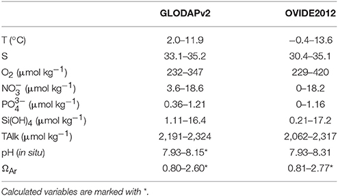
Table 1. Range of values between 0 and 3,500 m for all variables from GLODAPv2 and OVIDE2012 (Figure 1).

Relationships between GLODAPv2 Variables

The pairwise scatter plots for the GLODAPv2 variables; Ω_Ar, pH (in situ), TAlk, T, S, O₂, nutrients and P, and histograms for each of the variables are presented in Figure 3. Most of these variables and the relationships between them show variations with depth reflecting different biogeochemical regimes and the processes thorough the water column noted in the section on Depth Profiles of Variables. This suggests that depth is an important variable for constructing predictive algorithms. Based on examining depth profiles, we divided data into three depth layers (0–100, 100–500, 500–3,500 m) approximately reflecting the different biogeochemical regimes (euphotic zone, respiration/remineralization zone, and deep water). The depth division also allows for better visualization to highlight major features of variable inter-relationships and how they change with depth.

FIGURE 3

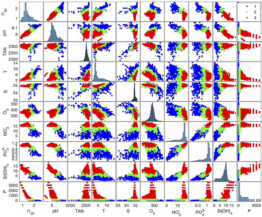
Figure 3. Pairwise scatter plots of GLODAPv2 data. Histograms of each variable are shown on the main diagonal. Scatter plots are color coded to show the variable values in three different depth layers: 0–100 m (blue), 100–500 m (green), 500–3500 m (red).

For individual variables, the histograms suggest non-symmetric distributions (excepting O₂), and sometimes are indicative of bi-modality (pH, T) due to the different depth regimes. Perhaps the most notable feature is the strong dependence (correlation) amongst the variables. Correlations of Ω_Ar with other variables (Figure 3, top panels) for the three depth layers are shown in Table 2. In the euphotic zone (0–100 m), we observe negative correlation of Ω_Ar with nutrients and O₂ and positive with pH reflecting biological uptake and photosynthesis. Positive correlations are also found with T, S (stoichiometric solubility is a function of T, S, P) and TAlk (affecting ${\text{CO}}_3^{2-}$). The strongest inter-correlations in this depth layer are found with T, TAlk, ${\text{PO}}_4^{3-}$, and Si(OH)₄ and moderate ones between pH, S, and O₂ and ${\text{NO}}_3^{-}$(Table 2). Note that the variables pH, O₂, and ${\text{NO}}_3^{-}$ are not included in CO₂SYS as input variables for calculating GLODAPv2 Ω_Ar. Correlations of similar strength and the same sign as above are found in 100–500 m layer, where photosynthesis is not present, but respiration and remineralization of nutrients and organic matter dominates. This implies similar stoichiometry of biological uptake and remineralization. Slightly stronger correlations with nutrients, in particular with ${\text{NO}}_3^{-}$, and weaker correlation with S are observed. In the deep layer (500–3,500 m) strong correlations are only found with variables that are changing at these depths; pH, T, and Si(OH)₄. The relationships between measured OVIDE2012 variables are consistent with those from GLODAPv2 (not shown).

TABLE 2

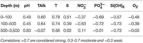
Table 2. Correlations (r) of GLODAPv2 variables with Ω_Ar for the three depth layers.

We also note that in the surface part of the euphotic zone (0–30 m), local heating/cooling, gas exchange and freshwater inputs may affect inorganic carbon and O₂, and decouple the O₂:CO₂ stoichiometry. This consequently could lead to different relationships between the variables at the surface (0–30 m) than those found in the remaining of euphotic zone below (30–100 m). For this reason, some of the previous studies (Juranek et al., 2009, 2011; Alin et al., 2012) excluded 0–30 and 0–15 m from their analysis. We found that regression coefficients were similar when excluding data from 0 to 30 m data and have, therefore, based the analysis on using all data from 0 to 100 m.

Algorithm Training: Estimating Ω_Ar Using Observations

Unsupervised Learning: MLR Applied to Training Data

All variables regression

When including all non-carbonate and autonomous sensor variables (0–3,500 m) in the model (Equation 2) the R² is very high (98%), and an F-test indicates that the overall regression is highly significant (p < 10⁻¹⁵). T-tests also show that all individual predictors are significant, with the exception of O₂. Figure 4 shows the R² from “all variables regression” for different combination of 1–8 predictor variables [T, S, P, O₂, pH, ${\text{NO}}_3^{-}$, ${\text{PO}}_4^{3-}$, Si(OH)₄]. This exercise indicates how, for a given level of complexity (or number of predictors), different combinations of variables affect the fit. It also provides information as to how adding and/or removing certain predictors can change the goodness of fit, which can be useful as guidance for a selection (and development) of additional sensors for existing platforms. The results suggest T and pH is the best combination of two key explanatory variables, which together can explain 95 % of variability in Ω_Ar, followed by a combination of P and ${\text{PO}}_4^{3-}$ (R² = 0.94). The best combination of three predictors are T, P, and ${\text{PO}}_4^{3-}$ (R² = 0.96), closely followed by T, pH, and ${\text{NO}}_3^{-}$, and the best four predictors are T, P, pH, and ${\text{PO}}_4^{3-}$ (R² = 0.98). The all variables regression suggests that T, P, pH, and ${\text{PO}}_4^{3-}$ are the most important predictors for Ω_Ar, although differences in R² are quite small.

FIGURE 4

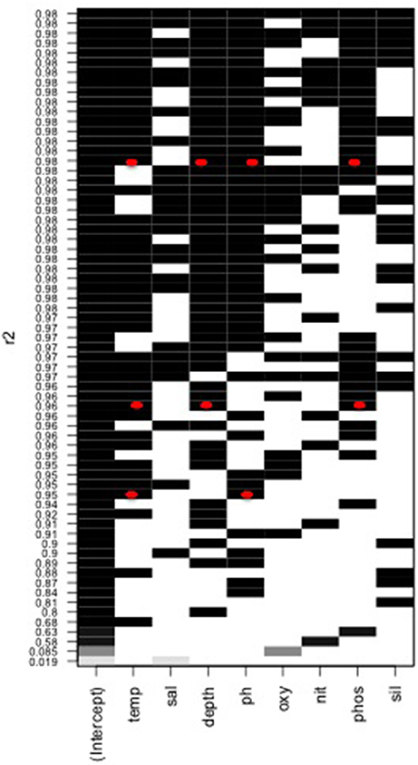
Figure 4. Goodness of fit (R²) for all variable subsets regression (0–3,500 m). Shown are the R² (in grayscale, and numerical y-axis) for regressions predicting Ω_Ar from different combinations of the 8 predictor variables used in Scenarios 1 and 2 [i.e., T, S, P, O₂, pH, ${\text{NO}}_3^{-}$, ${\text{PO}}_4^{3-}$, Si(OH)₄]. The regressions are ordered by increasing level of complexity with the bottom row representing a regression with a single predictor (here, an intercept β₀ and S), and the top row being a full regression with all eight predictor variables corresponding to Equation (2). For any given row, the shaded blocks indicate which predictor variables are included in the regression. The model complexity, or number of predictor variables included, increases from bottom to top. The top regression models (as measured by R²) for 2, 3, and 4 predictor variables are marked with red dots.

Stepwise regression

In all cases, the best regression model chosen by the various variable selection procedures (forward selection, backward elimination, and forward/backward combination) eliminated only the O₂ variable, with the final chosen model therefore being a regression of the response variable Ω_Ar on T, S, P, pH, ${\text{NO}}_3^{-}$, ${\text{PO}}_4^{3-}$, Si(OH)_4. It is likely that O₂ is eliminated by the selection procedures due to its relatively low correlation with Ω_Ar (Table 1) as well as its strong relationship with other predictor variables (Figure 3).

Supervised Learning: MLR Regression Scenarios

Table 3 gives a summary of the regression statistics based on GLODAPv2 data from 0 to 3,500 m for the three scenarios described in section Multiple Linear Regression (MLR) Algorithms (Training). We define the algorithm provides a “good” estimate of Ω_Ar when R² > 0.98 and RMSE < 0.05 (i.e., uncertainty in GLODAPv2 Ω_Ar) and an “adequate” estimate when R² > 0.95 and RMSE is smaller than 2x uncertainty in GLODAPv2 Ω_Ar (0.1).

TABLE 3

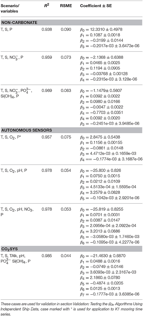
Table 3. Regression fit (R²) and root mean squared error (RSME), and regression coefficient ± standard error (SE) for different combination of non-carbonate, autonomous sensors and CO₂SYS variables from the GLODAPv2 data from 0 to 3,500 m (n = 1,631).

Scenario 1—non-carbonate

T and S alone are not “adequate” predictors of Ω_Ar, (R² = 0.822, RMSE = 0.153, not shown in Table 3). Inclusion of depth dependence through P improves the R² and RMSE, confirming depth is important predictor, but still does not yield an “adequate” estimate of Ω_Ar. The combination of T, S, ${\text{NO}}_3^{-}$, and P can “adequately” predict the Ω_Ar variable. ${\text{PO}}_4^{3-}$ is slightly better predictor than ${\text{NO}}_3^{-}$, and the combination of T, S, P, ${\text{NO}}_3^{-}$, and ${\text{PO}}_4^{3-}$ yields R² = 0.969, RMSE = 0.064 (not shown in Table 3). The addition of Si(OH)₄, does not significantly improve prediction. As with the “all variables regression,” this suggests that ${\text{PO}}_4^{3-}$ is the most important predictor nutrient in our study domain.

Scenario 2—autonomous sensors

Our results suggest that autonomous sensor measurements of T, S, P, and O₂ can provide “adequate” predictability of Ω_Ar for our study domain. Nitrate provides similar information as oxygen, while inclusions of pH improves predictability by a small amount suggesting it may be useful to add pH sensors on autonomous floats like Argo and moorings (K1, OSNAP, etc.). We also tested the use of apparent oxygen utilization (AOU), the difference between the measured O₂ concentration and its equilibrium saturation concentration, as a predictor variable instead of O₂. AOU is known to be a better metric for biological activity than O₂, but using AOU as a predictor variable did not improve the regression.

Scenario 3—CO₂SYS

The multiple regression model with input corresponding to the CO₂SYS input variables, yields “good” predictability (R² = 0.985, RMSE = 0.044). This is better than achieved in Scenario 1 and 2. This is an extremely good fit in terms for a linear regression model based on bin-averaged bottle data. The implication is that there is essentially a linear relation between Ω_Ar and the CO₂SYS inputs at least within the range of variations in the variable levels found within the study domain.

For simplicity, we focused mainly on the statistics of the least-squares regression fit and mostly avoided statistical inference (significance testing and p-values). Note that residuals plots however, were examined during model fitting and it was found that regression assumptions were mostly satisfied, excepting the violation of non-constant variance in some cases. This would normally be corrected by transformation, but such transformation would be case-specific and make algorithm comparison more difficult but is recommended when developing a targeted algorithm. Similarly, no attempts were made to include interaction terms or polynomial terms when building regression models. Our experience showed that little was to be gained from the addition of such complexity, and such models also suffer from difficulty in interpretation and exacerbate the effects of multicollinearity on the regression. The multicollinearity in the predictor variables is a ubiquitous feature in oceanographic problems and a consequence of a myriad of interacting physical-chemical processes, which dynamically link the variables. While complicating the interpretation of the statistical analysis, a positive effect of this variable dependence is that there is considerable flexibility in choosing predictor variables for empirical algorithms (i.e., the trading of ease of measurement vs. predictive skill).

Validation: Testing the Ω_Ar Algorithms Using Independent Ship Data

In this section, we assess how well the non-carbonate and autonomous sensor empirical algorithms, which were trained using the GLODAPv2 data normalized to 2002, are able to predict Ω_Ar for an independent data set, the OVIDE2012 cruise. Validation plots and corresponding quantitative metrics for the selected algorithms (Table 3) are presented in Figure 5 and Table 4. Overall, the validation plots in Figure 5 indicate a very good correspondence between the observed and predicted Ω_Ar. In all cases, the points cluster tightly near the 1:1 line indicating little bias and a small level of variability. The overall results in Table 4 also indicate successful validation with: (i) a correlation close to one, (ii) a consistently good fit (low RMSE), (iii) a small bias (AAE), but one that is slightly positive (AE), (iv) observations that differ from predictions by a factor close to one (RI); and (v) a model with consistent predictive skill (MEF between 0.5 and 1). Specific cases are discussed below.

FIGURE 5

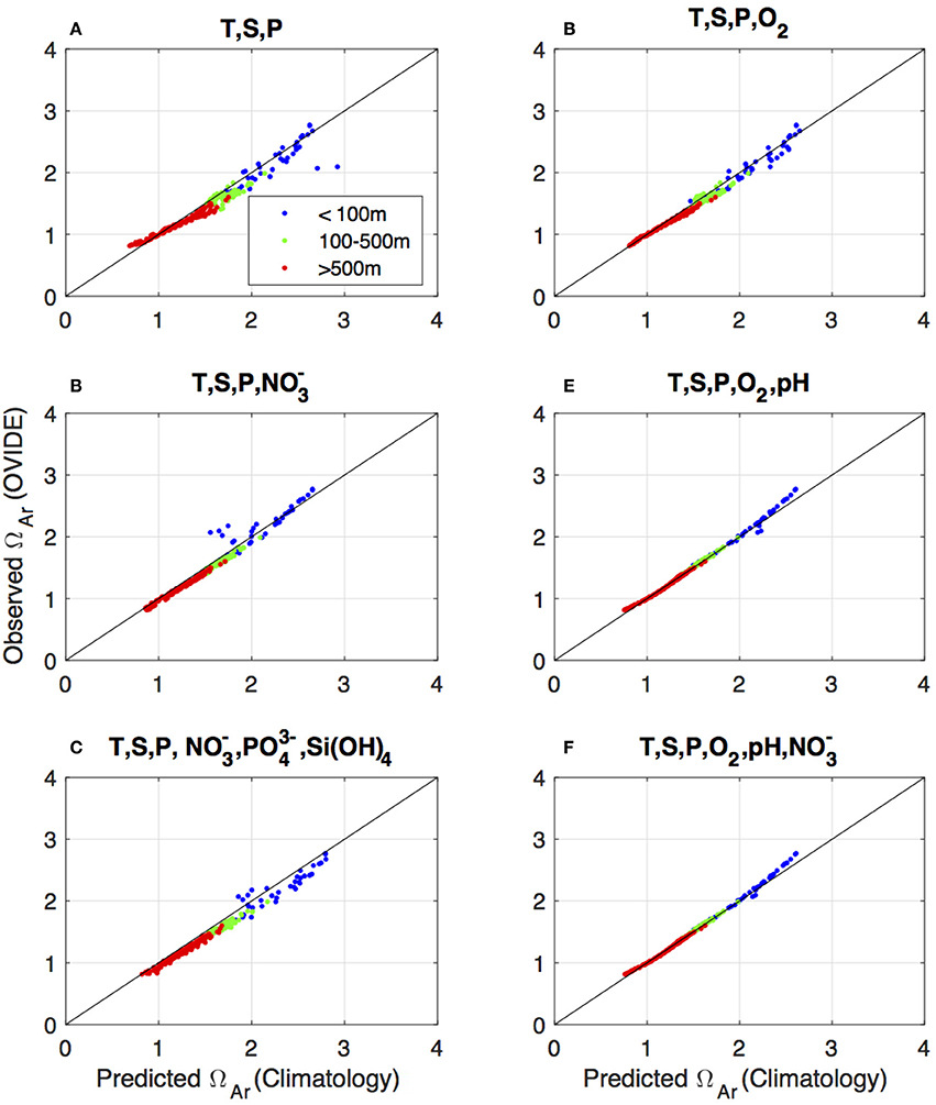
Figure 5. Validation plots of estimated Ω_Ar from empirical algorithms vs. observed Ω_Ar from OVIDE2012 cruise. These are done for different selections of non-carbonate (A–C) variables and autonomous sensor (D–F) variables. Observed refers to Ω_Ar calculated from OVIDE2012 pH and TAlk. The 1:1 line is shown in black.

TABLE 4

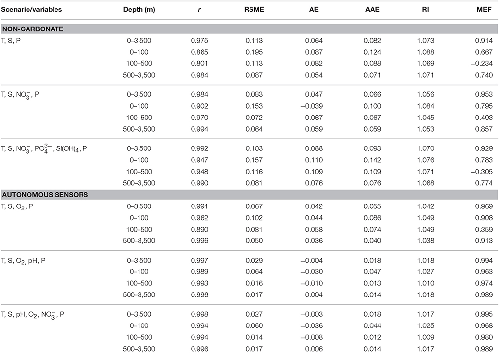
Table 4. Quantitative validation metrics: correlation (r), root mean squared error (RMSE), the reliability index (RI), the average error (AE), the average absolute error (AAE), and the modeling efficiency (MEF), all calculated according to Stow et al. (2009), for comparison of predicted Ω_Ar (Equation 2, with regression coefficients given in Table 3) with Ω_Ar calculated from observed TAlk and pH using CO₂SYS (n = 303).

Scenario 1—Non-Carbonate

For the non-carbonate scenario (Figures 5A–C, Table 4), the physical case (T, S, P) has the worst fit, particularly for the two shallowest depth layer (0–100 and 0–500 m) where oceanographic variability is highest. The addition of nitrate (the T, S, ${\text{NO}}_3^{-}$, P case) reduces the variability (r, RMSE) and bias (AE). Inclusion of the full nutrient suite [the T, S, P, ${\text{NO}}_3^{-}$, ${\text{PO}}_4^{3-}$, and Si(OH)₄ case] yields slightly degraded performance with increased bias.

Scenario 2—Autonomous Sensors

All three algorithms with autonomous sensors variables (Figures 5D–F, Table 4) have consistently good and quite similar overall predictability over the full water depth (0–3,500 m). The T, S, O₂, P algorithm has good performance in the deep layer (500–3,500 m) and may be sufficient for the prediction of Ω_Ar there, but has the lowest performance in the 0–100 and 0–500 m depth layer. The addition of pH in the 0–100 and 0–500 m provides an improvement, while little incremental improvement is achieved from the addition of ${\text{NO}}_3^{-}$. The algorithms that include pH have small negative bias in the upper two layers (0–100 and 0–500 m). The validation using OVIDE2012 pH corrected for the decadal decrease reported for Irminger Sea of −0.025 slightly increased the bias. The good predictability implies that the algorithms are insensitive to decadal anthropogenic changes in the carbonate system.

Application

Empirical algorithms trained on GLODAPv2 data (see Table 3) were applied to time series of T, S, O₂, and P at 10 and 100 m to estimate Ω_Ar at two sites: (1) Irminger Sea during 2010–2012 (Figures 6A–D, P not shown) and (2) K1 mooring in Labrador Sea during August 2014 to March 2015 (Figures 7A–D, P not shown). The regression equation used for this application is (see also Table 3):

$\begin{array}{l}{\Omega }_{\text{Ar}}=2.8475+0.1156\text{T}-0.0861\text{S}+\\ 4.4712\text{e-}03{\text{O}}_2-0.1774\text{e-}03\text{P}& (4)\end{array}$

FIGURE 6

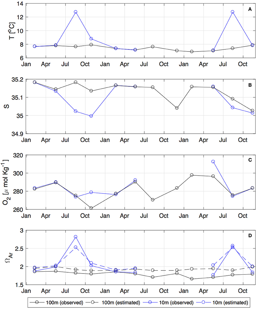
Figure 6. Time series of T, S, O₂ (A–C) at the Irminger Sea site (64.3°N, 28°W) at 10 and 100 m from 2010 to 2012. (D) Shows the values for Ω_Ar estimated from T, S, P, and O₂ using the empirical algorithm (Equation 3, dashed line) and observed Ω_Ar (full line). Observed refers to Ω_Ar calculated from pCO₂ and TCO₂.

At Irminger Sea site, we compared the estimated Ω_Ar using Equation (4) to Ω_Ar calculated from observations of TCO₂ and pCO₂ using CO₂SYS (Figure 6D). Calculated Ω_Ar showed good agreement with estimated values at both 10 and 100 m. Observations of inorganic carbon variables at K1 mooring location during our time-series observations were not available for comparison. To attempt to assess the validity of estimated Ω_Ar (Figure 7D), we compared our values to the Ω_Ar, calculated from observations of TCO₂ and TAlk at the station near the K1 mooring that have been collected on yearly spring (May/June) AR07W cruises since 1998 (https://www.nodc.noaa.gov/ocads/oceans/RepeatSections/clivar_ar07w.html). Consistent with our observations, Ω_Ar from 1998 to 2014 showed higher values at 10 m compared to 100 m. Large interannual variability was observed with Ω_Ar ranging between 2.7 and 1.5 at 10 m and between 2.0 and 1.5 at 100 m. Ω_Ar at both depths showed a decreasing trend. In May 2014, Ω_Ar, measured on AR07W2014 cruise (Yashayaev and Azetsu-Scott, 2016) showed values 1.72 at 10 m and 1.67 at 100 m, and decreasing to 0.8 at 3,500 m. This is consistent to what would be expected for Ω_Ar, based on our algorithm (Equation 4). However direct comparison is not possible since the K1 mooring data was not available in May 2014. We further compared our Ω_Ar to the literature values in the Labrador Sea (Azetsu-Scott et al., 2010) and Ω_Ar calculated from pH and TAlk on Redfish cruises (June/July 2013, unpublished data) from the region west from the K1 mooring. Both show summer values of Ω_Ar around 2.4, consistent with our estimates. Our observation emphasize the need for pH sensors on moorings in the area.

FIGURE 7

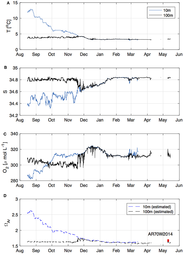
Figure 7. Time series of T, S, O₂ (A–C) at the K1 mooring (56.5°N, 52.6°W) at 10 and 100 m from August 2014 to May 2015. (D) shows the values for Ω_Ar estimated from T, S, P, and O₂ using the empirical algorithm (Equation 3). Red square is a value of observed Ω_Ar at the station near K1 during May 2014 from AR70W2014 cruse. Observed refers to Ω_Ar calculated from TAlk and TCO₂.

As expected, estimated Ω_Ar at 10 m depth exhibits seasonal variability at both sites, Irminger Sea and K1 mooring, with highest values in August (around 2.5) due to biological drawdown of inorganic carbon during the summer. Ω_Ar then gradually decreased and showed lowest values at Irminger in February (around 1.9). At the K1 mooring Ω_Ar decreased to 1.5–1.6 in December, and continued to stay at this value through the winter. At 100 m, estimated Ω_Ar remained at values between 1.9 and 2.0 at Irminger site, and 1.5 and 1.7 at K1 mooring without seasonal variation, which indicates biological uptake at this depth was negligible. Similar values of Ω_Ar at 10 and 100 m during the winter are expected due to mixing of surface water down to various depths during convection in the area, which results in fairly uniform Ω_Ar values over the convection depth (Azetsu-Scott et al., 2010). During winter of 2014, an extreme convection event occurred and extended to about 1,700 m (Yashayaev and Loder, 2016), so presumably the surface values of Ω_Ar from K1 mooring could be representative of the water column down to that depth.

We have also applied empirical algorithms from previous studies that used T, S, O₂, and P or T, O₂, and P to predict Ω_Ar along the central Oregon coast (Juranek et al., 2009; Figure 8, red line) and in the Sea of Japan (Kim et al., 2010; Figure 7, black lines). These algorithms either under-predict or over-predict the known values of Ω_Ar in our study domain by a significant amount (more than 0.5). This confirms the need for development of regionally specific algorithms. A caveat of our approach is the use of seasonally biased (mainly summer) climatological data to train the algorithms and summer ship data to validate them.

FIGURE 8

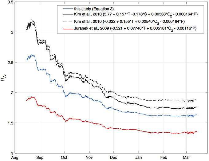
Figure 8. Ω_Ar estimated from time series of T, S, O₂, and P (or T, O₂, and P) at the K1 mooring (56.5°N, 52.6°W) at 10 m depth from August 2014 to March 2015 using three different empirical algorithms from: (a) this study, Equation 4 (blue line), (b) central Oregon coast (Juranek et al., 2009) (red line), and (c) the Sea of Japan (Kim et al., 2010) (black lines).

Conclusions

Our study suggests that linear regression models (empirical algorithms) based on the GLODAPv2 data bin-averaged in 1° × 1° cells can successfully be used to estimate Ω_Ar in the North Atlantic Subpolar region. Another key feature is in producing reliable error bounds for any estimates of Ω_Ar. Algorithms based on non-carbonate variables indicate that Ω_Ar can be predicted well from entirely non-carbonate observations, with ${\text{PO}}_4^{3-}$ being the best nutrient predictor. Algorithms using autonomous sensor variables emphasize the importance of adding pH sensors on autonomous floats like Argo and moorings (K1, OSNAP, etc.), in particular in the euphotic and remineralization zone. In deeper water, observations of T, S, and O₂ may be sufficient for predicting Ω_Ar. Different regression model building strategies suggest ${\text{PO}}_4^{3-}$ measurements are desirable. It appears that there is essentially a linear relation between Ω_Ar and the CO₂SYS input variables at least within the range of variations in the variable levels found here.

Validation with independent ship data showed good correspondence, with small bias and variability. Since the anthropogenic trend in Ω_Ar has been removed, the algorithms have no temporal component to them (i.e., no time variable as predictor). Nevertheless, the validation with OVIDE2012 data show that the algorithms trained on 2002 data manage to successfully estimate Ω_Ar in 2012. This shows the robustness of the algorithms to changes over a short time interval (such as a decade).

The empirical algorithms also performed well even though they are being applied outside the range of values used to train the algorithms. This suggests that, while they are regional algorithms, they may have much broader spatial applicability. Future work seeks to identify appropriate biogeochemical provinces for which a regional algorithm is valid. Since the relationship of variables with Ω_Ar may be correlative, rather than directly causal, emphasis must be on validating predictive skill using independent data.

Application to Station K1 time series, as well as time series from the Irminger Sea suggest the potential for regionally tuned algorithms, but they need to validate against measured Ω_Ar to properly assess their performance. Finally, algorithms require evolution and recalibration by ongoing periodic carbon-dedicated cruises in order to account for secular trends in anthropogenic CO₂.

Author Contributions

DT: Lead the research and writing of the manuscript; MD: Contributed to analysis of the data and writing of the paper; SKL: Provided guidance with GLODAPv2 data and contributed to writing of the paper; JK: Provided mooring data and comments; FA-P and FP: Collected and analyzed shipboard data and provided comments. All authors contributed to proofing of the manuscript.

Funding

MD was supported by an NSERC Discovery Grant, and SKL was supported by the EU H2020 research and innovation project AtlantOS (grant agreement no 633211). The OVIDE-12 cruise and the contribution of FA-P and FP were supported by the Spanish Ministry of Economy and Competitiveness through the project CTM2013-41048-P co-funded by the Fondo Europeo de Desarrollo Regional 2014-2020 (FEDER). K1 mooring is an Oceansites site supported by the EU Horizon 2020 research and innovation program AtlantOS (grant agreement no 633211). LDEO contribution no 8169.

Conflict of Interest Statement

The authors declare that the research was conducted in the absence of any commercial or financial relationships that could be construed as a potential conflict of interest.

Acknowledgments

We are grateful to D.W.R. Wallace and CERC.OCEAN, and S. Gulev for their contributions at the initial stages of this study, and J. Olafsson, and S.R. Olafsdottir for making the Irminger Sea site data publicly available. We thank the editor and two reviewers whose comments greatly helped to improve this manuscript.

References

Alin, S. R., Feely, R. A., Dickson, A. G., Hernández-Ayón, J. M., Juranek, L. W., Ohman, M. D., et al. (2012). Robust empirical relationships for estimating the carbonate system in the southern California Current System and application to CalCOFI hydrographic cruise data (2005–2011). J. Geophys. Res. 117:C05033. doi: 10.1029/2011JC007511

CrossRef Full Text | Google Scholar

Allen, J. I., Holt, J. T., Blackford, J., and Proctor, R. (2007). Error quantification of a high-resolution coupled hydrodynamic-ecosystem coastal-ocean model: part 2. Chlorophyll-a, nutrients and SPM. J. Mar. Syst. 68, 381–404. doi: 10.1016/j.jmarsys.2007.01.005

CrossRef Full Text

Azetsu-Scott, K., Clarke, A., Falkner, K., Hamilton, J., Jones, E. P., Lee, C., et al. (2010). Calcium carbonate saturation states in the waters of the Canadian Arctic Archipelago and the Labrador Sea. J. Geophys. Res. 115:C11021. doi: 10.1029/2009JC005917

CrossRef Full Text

Barbero, L., Boutin, J., Merlivat, L., Martin, N., Takahashi, T., Sutherland, S., et al. (2011). Importance of water mass formation regions for the air-sea CO₂ flux estimate in the Southern Ocean. Glob. Biogeochem. Cycles 25:GB1005. doi: 10.1029/2010GB003818

CrossRef Full Text

Bates, N. R., Astor, Y. M., Church, M. J., Currie, K., Dore, J. E., González-Dávila, M., et al. (2014). A time-series view of changing ocean chemistry due to ocean uptake of anthropogenic CO₂ and ocean acidification. Oceanography 27, 126–141. doi: 10.5670/oceanog.2014.16

CrossRef Full Text | Google Scholar

Bostock, H. C., Mikaloff Fletcher, S. E., and Williams, M. J. M. (2013). Estimating carbonate parameters from hydrographic data for the intermediate and deep waters of the Southern Hemisphere oceans. Biogeosciences 10, 6199–6213. doi: 10.5194/bg-10-6199-2013

CrossRef Full Text | Google Scholar

Box, G. E. P., Jenkins, G. M., and Reinsel, G. C. (1994). Time Series Analysis: Forecasting and Control, 3rd Edn. Englewood Cliffs, NJ: Prentice Hall.

Google Scholar

Carter, B. R., Feely, R. A., Mecking, S., Cross, J. N., Macdonald, A. M., Siedlecki, S. A., et al. (2017). Two decades of Pacific anthropogenic carbon storage and ocean acidification along Global ocean ship-based hydrographic investigations program sections P16 and P02. Glob. Biogeochem. Cycles 31, 306–327. doi: 10.1002/2016GB005485

CrossRef Full Text | Google Scholar

Clayton, T. D., and Byrne, R. H. (1993). Spectrophotometric seawater pH measurements: total hydrogen ion concentration scale calibration of m-cresol purple and at-sea results. Deep Sea Res. I 40, 2115–2129. doi: 10.1016/0967-0637(93)90048-8

CrossRef Full Text | Google Scholar

DeGrandpre, M. D., Körtzinger, A., Send, U., Wallace, D. W. R., and Bellerby, R. G. J. (2006). Uptake and sequestration of atmospheric CO₂in the Labrador Sea deep convection region. Geophys. Res. Lett. 33:L21S03. doi: 10.1029/2006GL026881

CrossRef Full Text

Dickson, A. (1990). Standard potential of the reaction: AgCl (s) + 1/2H2(g) = Ag (s) + HCl (aq), and the standard acidity constant of the ion HSO−4 in synthetic sea water from 273.15 to 318.15 K. J. Chem. Thermodyn. 22, 113–127. doi: 10.1016/0021-9614(90)90074-Z

CrossRef Full Text | Google Scholar

Dickson, A. G., Sabine, C. L., and Christian, J. R. (2007). Guide to Best Practices for Ocean CO₂ Measurements. PICES Spec. Publ., 3. Sidney, BC: North Pacific Marine Science Organization, p. 191.

Google Scholar

Fröb, F., Olsen, A., Pérez, F. F., García-Ibáñez, M. I., Jeansson, E., Omar, A., et al. (accepted). Inorganic carbon water masses in the Irminger Sea since 1991. Biogeosci. Discuss. doi: 10.5194/bg-2017-27

CrossRef Full Text

García-Ibáñez, M. I., Zunino, P., Fröb, F., Carracedo, L. I., Ríos, A. F., Mercier, H., et al. (2016). Ocean acidification in the subpolar North Atlantic: rates and mechanisms controlling pH changes, Biogeosciences 13, 3701–3715. doi: 10.5194/bg-13-3701-2016

CrossRef Full Text | Google Scholar

Hall, T. M., Haine, T. W. N., and Waugh, D. W. (2002). Inferring the concentration of anthropogenic carbon in the ocean from tracers. Glob. Biogeochem. Cycles 16:1131. doi: 10.1029/2001gb001835

CrossRef Full Text | Google Scholar

Hastie, T., Tibshirani, R., and Friedman, J. (2009). The Elements of Statistical Learning. New York, NY: Springer-Verlag.

Google Scholar

IPCC (2013). “Climate change 2013: the physical science basis,” in Contribution of Working Group I to the Fifth Assessment Report of the Intergovernmental Panel on Climate Change, eds T. F. Stocker, D. Qin, G. K. Plattner, M., Tignor, S. K. Allen, J. Boschung, A. Nauels, Y. Xia, V. Bex, and P. M. Midgley (Cambridge; New York, NY: Cambridge University Press), 1535.

Jackson, L. C., Peterson, K. A., Roberts, C. D., and Wood, R. A. (2016). Recent slowing of Atlantic overturning circulation as a recovery from earlier strengthening. Nat. Geosci. 9, 518–522. doi: 10.1038/ngeo2715

CrossRef Full Text | Google Scholar

Juranek, L. W., Feely, R. A., Gilbert, D., Freeland, H., and Miller, L. A. (2011). Real-time estimation of pH and aragonite saturation state from Argo profiling floats: prospects for an autonomous carbon observing strategy. Geophys. Res. Lett. 38:L17603. doi: 10.1029/2011GL048580

CrossRef Full Text | Google Scholar

Juranek, L. W., Feely, R. A., Peterson, W. T., Alin, S. R., Hales, B., Lee, K., et al. (2009). A novel method for determination of aragonite saturation state on the continental shelf of central Oregon using multi-parameter relationships with hydrographic data. Geophys. Res. Lett. 36:L24601. doi: 10.1029/2009GL040778

CrossRef Full Text | Google Scholar

Kim, T.-W., Lee, K., Feely, R. A., Sabine, C. L., Chen, C. T. A., Jeong, H., et al. (2010). Prediction of Sea of Japan (East Sea) acidification over the past 40 years using a multiparameter regression model. Glob. Biogeochem. Cycles 24:GB3005. doi: 10.1029/2009GB003637

CrossRef Full Text | Google Scholar

Koelling, J., Wallace, D. W. R., Send, U., and Karstensen, J. (2017). Intense oceanic uptake of oxygen during 2014–2015 winter convection in the Labrador Sea. Geophys. Res. Lett. 44, 7855–7864. doi: 10.1002/2017GL073933

CrossRef Full Text | Google Scholar

Lauvset, S. K., Key, R. M., Olsen, A., van Heuven, S., Velo, A., Lin, X., et al. (2016). A new global interior ocean mapped climatology: the 1°x1° GLODAP version 2. Earth Syst. Sci. Data 8, 325–340. doi: 10.5194/essd-8-325-2016

CrossRef Full Text | Google Scholar

Lee, K., Tong, L. T., Millero, F. J., Sabine, C. L., Dickson, A. G., Goyet, C., et al. (2006). Global relationships of total alkalinity with salinity and temperature in surface waters of the world's oceans. Geophys. Res. Lett. 33:L19605. doi: 10.1029/2006GL027207

CrossRef Full Text | Google Scholar

Lewis, E., and Wallace, D. W. R. (1998). Program Developed for CO₂ System Calculations. ORNL/CDIAC-105, Carbon Dioxide Information Analysis Center, Oak Ridge National Laboratory, US Department of Energy, Oak Ridge, TN.

Google Scholar

Longhurst, A. (1995). Seasonal cycles of pelagic production and consumption. Prog. Oceanogr. 36, 77–167. doi: 10.1016/0079-6611(95)00015-1

CrossRef Full Text | Google Scholar

Lueker, T. J., Dickson, A. G., and Keeling, C. D. (2000). Ocean pCO₂ calculated from dissolved inorganic carbon, alkalinity, and equations for K-1 and K-2: validation based on laboratory measurements of CO₂ in gas and seawater at equilibrium. Mar. Chem. 70, 105–119. doi: 10.1016/S0304-4203(00)00022-0

CrossRef Full Text | Google Scholar

Mintrop, L., Pérez, F. F., González-Dávila, M., Santana-Casiano, J. M., and Körtzinger, A. (2000). Alkalinity determination by potentiometry: intercalibration using three different methods. Cienc. Mar. 26, 23–37. doi: 10.7773/cm.v26i1.573

CrossRef Full Text | Google Scholar

Montgomery, D. C., Peck, E. A., and Vining, G. G. (2015). Introduction to Linear Regression Analysis. Hoboken, NJ: John Willey & Sons Inc.

Google Scholar

Nondal, G., Bellerby, R. G. J., Olsen, A., Johannessen, T., and Olafsson, J. (2009). Optimal evaluation of the surface ocean CO₂ system in the northern North Atlantic using data from voluntary observing ships. Limnol. Oceanogr. Methods 7, 109–118. doi: 10.4319/lom.2009.7.109

CrossRef Full Text | Google Scholar

Olafsson, J. (2016). Partial Pressure (Or Fugacity) of Carbon Dioxide, Dissolved Inorganic Carbon, Temperature, Salinity and Other Variables Collected from Discrete Sample and Profile Observations Using CTD, Bottle and Other Instruments from ARNI FRIDRIKSSON and BJARNI SAEMUNDSSON in the North Atlantic Ocean from 1983-03-05 to 2013-11-13 (NCEI Accession 0149098). Version 1.1. NOAA National Centers for Environmental Information. Dataset.

Olafsson, J., Olafsdottir, S. R., Benoit-Cattin, A., and Takahashi, T. (2009). The Irminger Sea and the Iceland Sea timeseries measurements of sea water carbon and nutrient chemistry 1983–2006. Earth Syst. Sci. Data Discuss. 2, 477–492. doi: 10.5194/essdd-2-477-2009

CrossRef Full Text | Google Scholar

Olsen, A., Key, R. M., van Heuven, S., Lauvset, S. K., Velo, A., Lin, X., et al. (2016). The Global Ocean Data Analysis Project version 2 (GLODAPv2) – an internally consistent data product for the world ocean. Earth Syst. Sci. Data 8, 297–323. doi: 10.5194/essd-8-297-2016

CrossRef Full Text

Pérez, F. F. (2016). Atlantic Ocean acidification. Front. Mar. Sci. Conference Abstract: XIX Iberian Symposium on Marine Biology Studies. doi: 10.3389/conf.FMARS.2016.05.00093

PubMed Abstract | CrossRef Full Text

Pérez, F. F., and Fraga, F. (2007). A precise and rapid analytical procedure for alkalinity determination. Mar. Chem. 21, 169–182. doi: 10.1016/0304-4203(87)90037-5

CrossRef Full Text

Pérez, F. F., Vázquez-Rodríguez, M., Louarn, E., Padin, X. A., Mercier, H., and Rios, A. F. (2008). Temporal variability of the anthropogenic CO₂ storage in the Irminger Sea. Biogeosciences 5, 1669–1679. doi: 10.5194/bg-5-1669-2008

CrossRef Full Text | Google Scholar

Plancherel, Y., Rodgers, K. B., Key, R. M., Jacobson, A. R., and Sarmiento, J. L. (2013). Role of regression model selection and station distribution on the estimation of oceanic anthropogenic carbon change by eMLR. Biogeosciences 10, 4801–4831, doi: 10.5194/bg-10-4801-2013

CrossRef Full Text | Google Scholar

Ragueneau, O., Gallinari, M., Stahl, H., Tengberg, A., Grandel, S., Lampitt, R., et al. (2001). The benthic silica cycle in the northeast Atlantic: seasonality, annual mass balance and preservation mechanisms. Progr. Oceanogr. 50, 171–200. doi: 10.1016/S0079-6611(01)00053-2

CrossRef Full Text

Sabine, C. L., Feely, R. A., Gruber, N., Key, R. M., Lee, K., Bullister, J. L., et al. (2004). The oceanic sink for anthropogenic CO2. Science 305, 367–371. doi: 10.1126/science.1097403

PubMed Abstract | CrossRef Full Text | Google Scholar

Stow, C., Jolliff, J. Jr., McGillicuddy, D. J. Jr., Doney, S., Allen, J., Friedrichs, M. A. M., et al. (2009). Skill assessment for coupled biologi- cal/physical models of marine systems. J. Mar. Syst. 76, 4–15, doi: 10.1016/j.jmarsys.2008.03.011

PubMed Abstract | CrossRef Full Text | Google Scholar

Uppström, L. R. (1974). Boron/chlorinity ratio of deep-sea water from the Pacific Ocean. Deep Sea Res. 21, 161–162. doi: 10.1016/0011-7471(74)90074-6

CrossRef Full Text

van Heuven, S., Pierrot, D., Lewis, E., and Wallace, D. (2009). MATLAB Program Developed for CO2 System Calculations. ORNL/CDIAC-105b, Carbon Dioxide Information Analysis Center, Oak Ridge National Laboratory, US Department of Energy, Oak Ridge, TN.

Vazquez-Rodriguez, M., Perez, F. F., Velo, A., Rios, A. F., and Mercier Herle (2012). Observed acidification trends in North Atlantic water masses. Biogeosciences 9, 5217–5230. doi: 10.5194/bg-9-5217-2012

CrossRef Full Text | Google Scholar

Waugh, D. W., Hall, T. M., McNeil, B. I., Key, R., and Matear, R. J. (2006). Anthropogenic CO2 in the oceans estimated using transit time distributions. Tellus 58B, 376–389. doi: 10.1111/j.1600-0889.2006.00222.x

CrossRef Full Text | Google Scholar

Williams, N. L., Juranek, L. W., Johnson, K. S., Feely, R. A., Riser, S. C., Talley, L. D., et al. (2016). Empirical algorithms to estimate water column pH in the Southern Ocean. Geophys. Res. Lett. 43, 3415–3422. doi: 10.1002/2016GL068539

CrossRef Full Text | Google Scholar

Yashayaev, I., and Azetsu-Scott, K. (2016). Dissolved Inorganic Carbon, pH, Alkalinity, Temperature, Salinity and Other Variables Collected From Discrete Sample and Profile Observations Using Alkalinity titrator, CTD and Other Instruments from HUDSON in the Davis Strait, Labrador Sea and North Atlantic Ocean from 2014-05-02 to 2014-05-24 (NCEI Accession 0157623). Version 1.1. NOAA National Centers for Environmental Information. Dataset.

Yashayaev, I., and Loder, J. W. (2016). Recurrent replenishment of Labrador Sea water and associated decadal-scale variability. J. Geophys. Res. Oceans 121, 8095–8114. doi: 10.1002/2016JC012046

CrossRef Full Text | Google Scholar