Satellite Radiation Products for Ocean Biology and Biogeochemistry: Needs, State-of-the-Art, Gaps, Development Priorities, and Opportunities

Introduction

From the point of view of biology and chemistry, solar radiation in the photosynthetically active range (roughly 400–700 nm), referred to as PAR, controls the growth of aquatic plants (e.g., Ryther, 1956; Platt et al., 1977; Kirk, 1994; Falkowski and Raven, 1997). It ultimately regulates the composition and dynamics of marine ecosystems. Solar radiation in the ultraviolet (UV) (280–400 nm), by damaging cellular constituents, may stress phytoplankton and inhibit their growth (e.g., Cullen and Neale, 1994; Häder et al., 2011). UV light, via photo-oxidation of colored dissolved organic matter (CDOM), may increase the bioavailability of nutrients (Sulzberger and Durisch-Kaiser, 2009). In the process, absorption by CDOM is reduced, increasing light penetration. Knowing the distribution (spectral, spatial, and temporal) of UV and visible solar radiation in the upper ocean is critical to understanding biogeochemical cycles of carbon, nutrients, and oxygen, and to addressing climate and global change issues, such as the fate of anthropogenic atmospheric carbon dioxide (CO₂).

From the point of view of physics, sunlight absorbed by phytoplankton and other water constituents (CDOM, mineral particles, etc.) heats the upper ocean and distributes heat horizontally and vertically, affecting mixed-layer dynamics and oceanic circulation (e.g., Nakamoto et al., 2000, 2001; Ballabrera-Poy et al., 2007). These changes in turn influence atmospheric temperature and circulation, with remote effects (Miller et al., 2003; Shell et al., 2003). Solar radiation diffusely reflected by the ocean also affects the outgoing radiative flux from the planet (planetary albedo), with climate consequences (Frouin and Iacobellis, 2002). In order to make predictions for future conditions, we need to get some idea of how the phytoplankton concentrations and optical properties will evolve with changing conditions. Many processes and feedbacks in which solar radiation absorption plays a role are involved and difficult to untangle, and a large fraction of the uncertainties in projections of future climate is associated with physical-biological interactions (Friedlingstein et al., 2006).

This article reviews operational satellite radiation products, the user needs and gaps, and it provides a scientific roadmap for the use of, and priorities for improving existing products and developing new products, i.e., for closing the gaps in ocean biology and biogeochemistry, including studies of biological-physical interactions and feedbacks. This roadmap emerged from the presentations (oral and poster) and discussions during the Color and Light in the Ocean from Earth Observation (CLEO) workshop at ESRIN, Frascati, Italy on 6–8 September 2016. The following questions are addressed: (1) Do existing shortwave downward flux products meet the requirements of the dynamics and bio-geochemical communities? What can be done to serve better the needs of the user community in general and the modeling community in particular? (2) What additional products should be added to the processing streams to increase their usefulness? What should be the characteristics of these products in terms of temporal, spatial, and spectral resolution, spectral range, and accuracy? (3) What are the needs in terms of harmonization between sensors, methodologies, ancillary data and radiative transfer tools?

Current Products

The underwater light field is defined at any point in space by the spectral radiance (W/m²/sr/nm) from all directions. Useful properties can be derived from radiance, i.e., planar and scalar irradiance, average cosine, reflectance, and vertical attenuation coefficient (see, e.g., Mobley, 1994 or Kirk, 1994 for definitions). Only a few of these properties are presently inferred reliably and operationally from space, namely daily above-surface downward planar irradiance integrated from 400 to 700 nm (known as “daily PAR product”), above-surface planar spectral UV irradiance at noon, spectral reflectance of the water body, and diffuse attenuation coefficient at 490 nm (derived from water reflectance). These products are generated for each ocean color mission individually (note that UV products are not available in standard ocean-color missions).

Examples of level-3 daily, weekly, and monthly above-surface PAR products at 9 km resolution from MODIS-Aqua data are displayed in Figure 1. Dates are March 22, March 22–29, and March 1–31, 2010, respectively. The NASA Ocean Color Biology Group (OBPG) in Greenbelt, Maryland generates and archives these products operationally. Typical uncertainty (RMS) is ±6.5 (19%), ±4.2 (12%), and ±2.6 Em⁻²d⁻¹ (7%) for daily, weekly, and monthly estimates (Frouin et al., 2012). The daily maps exhibit missing values, especially at low latitudes, due to the limited spatial coverage of the instruments, but the weekly and a fortiori monthly maps are completely filled, except at latitudes where the Sun zenith angle at the time of satellite overpass is above 75 degrees, since the data is discarded in the OBPG ocean-color processing line. The weekly and monthly PAR fields exhibit similar patterns, but the monthly product is smoother (lower variability at small scales), which is expected when the averaging period is longer.

FIGURE 1

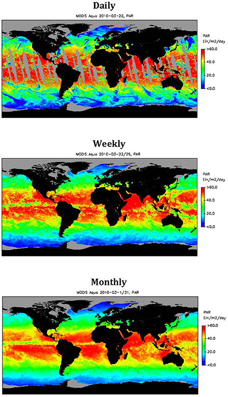
Figure 1. Daily, weekly, and monthly above-surface PAR at 9 km resolution, derived from MODIS-Aqua. Top: March 22, 2010; Middle: March 22-29, 2010; Bottom: March 1–31, 2010 (From NASA OBPG).

The corresponding maps of level-3 daily, weekly, and monthly diffuse attenuation coefficient (K_d) at 490 nm, also produced by the OBPG, are displayed in Figure 2. RMS uncertainty on log-transformed instantaneous estimates is about ±0.1 (e.g., Morel et al., 2007). Since K_d is only retrieved in clear sky conditions, the daily map has many gaps (only about 10–15 % of the observed pixels typically pass through the strict glint and cloud filters), and the weekly product show many areas with no information. On a monthly time scale, information is still missing at low latitudes. The spatial gaps limit considerably the utility of the K_d retrievals for propagating light below the surface. In the open ocean, global coverage every 3–5 days is necessary to resolve variability associated with seasonal biological phenomena such as phytoplankton blooms. In coastal waters, wind forcing create “events” (e.g., upwelling) that occur every 2–10 days, and 1-day coverage is the requirement for resolving the event time scale.

FIGURE 2

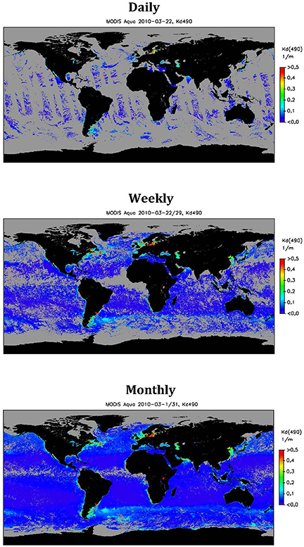
Figure 2. Daily, weekly and monthly K_d at 9 km resolution, derived from MODIS-Aqua. Top: March 22, 2010; Middle: March 22–29, 2010; Bottom: March 1–31, 2010 (From NASA OBPG).

Figure 3 provides examples of level 3 daily, weekly, and monthly maps of noon surface UV irradiance at 1° resolution and 324 nm from OMI-Aura. Irradiance at 305, 310, and 380 nm as well as erythemally weighted daily dose and erythemal dose rate are also available. Dates are the same as those of Figure 1. The data are routinely processed at the OMI Science Investigator-led Processing System (SIPS) Facility in Greenbelt, Maryland, and are archived at the NASA Goddard Earth Sciences Data and Information Services Center (GES DISC). Overall uncertainty of UV irradiance estimates ranges from ±5 to over ±30%, depending on atmospheric conditions and geolocation (e.g., Arola et al., 2009). The UV irradiance and PAR fields have similar spatial coverage (Figures 1, 3), with missing values due to instrument swath on a daily time scale, except that UV irradiance estimates are obtained at high latitudes. Variability patterns are also similar, since UV irradiance variability is also governed by Sun zenith angle and cloudiness, although ozone absorption plays a bigger role in modulating the surface values (but gradients of total ozone content remain mostly latitudinal). Spatial resolution is coarser than for the MODIS products (OMI sensor footprint is 13 × 24 km²), and no daily-averaged values (only daily values at noon or overpass time) are generated.

FIGURE 3

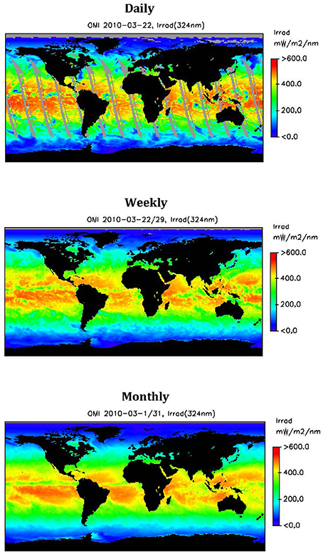
Figure 3. Daily, weekly and monthly noon above-surface UV irradiance at 1° resolution, derived from OMI-Aura. Top: March 22, 2010; Middle: March 22–29, 2010; Bottom: March 1-31, 2010. (From NASA GES DISC).

The situation regarding spatial coverage is summarized in Figure 4, which displays the percentage of the ocean surface covered by PAR, K_d, and UV irradiance products on daily, weekly, and monthly time scales (imagery of Figures 1–3). In the equatorial region, percent coverage is 65, 80, and 5% for daily PAR, UV irradiance at 324 nm, and K_d, respectively. It is increased to 100% for weekly and monthly PAR and UV irradiance, and to 30 and 70% for weekly and monthly K_d. In middle latitude regions, daily coverage is almost 100% for PAR, about 80% for UV irradiance, and 15–20% for K_d. Weekly and monthly coverage is 100% for PAR and UV irradiance, and reaches 70–75 and 100% in sub-tropical regions for K_d. At high latitudes (>70°), monthly coverage is <40% for PAR and K_d. This lack of coverage is limiting in view of the large productivity of high latitude marine ecosystems (Southern ocean, Arctic ocean). Furthermore, monthly K_d products may only contain estimates during a few days, and therefore may not represent accurately actual monthly values in dynamic regions (IOCCG, 2015).

FIGURE 4

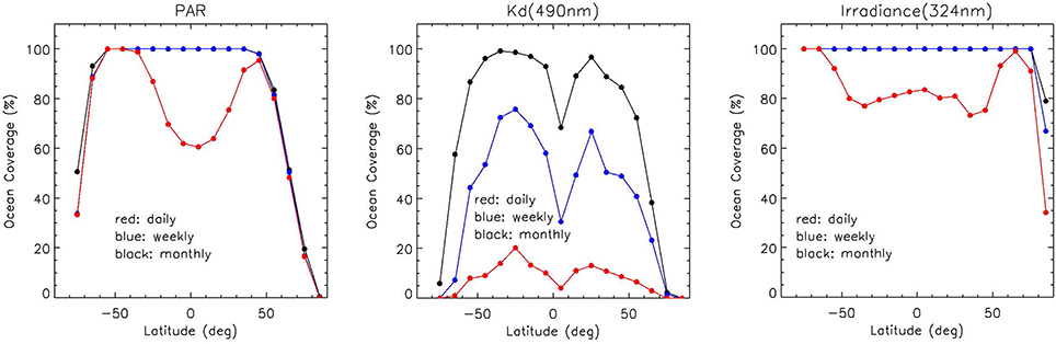
Figure 4. Percentage of the ocean surface covered by (Left) PAR, (Middle) K_d, and (Right) noon irradiance products on daily, weekly, and monthly time scales, i.e., March 22, March 22–29, and March 1–31, 2010. Situation is dramatic for K_d, which is only retrieved in clear-sky conditions (<15% coverage at most latitudes).

Multiple satellites can improve the daily ocean coverage, especially for K_d (can only be retrieved in clear sky conditions). For example, three instruments of MODIS type, flying in a constellation on satellite orbits differing by the mean anomaly (angular distance from pericenter), would increase the daily spatial coverage of water reflectance, therefore K_d, from 15 to 25% over 1 day and from 40 to 60% over 4 days (Gregg et al., 1998). Figure 5 shows, for March 22, 2010, the increase in daily ocean coverage obtained by combining estimates from MODIS-Aqua (overpass at 13:30 local time) and –Terra (overpass at 10:30 local time) instead of using MODIS-Aqua only. For PAR, the increase is from 60 to 80% in equatorial regions, and complete coverage is reached at sub-tropical latitudes. For K_d, the ocean coverage is more than doubled at most latitudes (e.g., 35–50%, instead of 15–20% in the sub-tropics). Combining PAR estimates from instruments orbiting at different times not only increases spatial coverage, but perhaps more importantly, also takes into account cloud diurnal variability, yielding more accurate estimates.

FIGURE 5

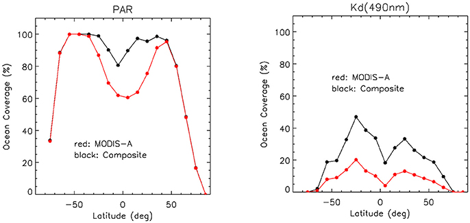
Figure 5. Percentage of ocean coverage by daily PAR and K_d products when using MODIS-Aqua data only (red curves) and combining MODIS-Aqua and -Terra data (black curves). Date is March 22, 2010. Coverage is almost total (>80%) in low to middle latitude regions for PAR (left) and at least doubled at most latitudes for K_d (right).

Satellite instruments in geostationary orbit, by observing the same target multiple times during the day (e.g., every 30 min for GOCI onboard COMS and 10 min for AHI onboard Hiwamari-8) offer an efficient way to account for diurnal changes in cloudiness in daily PAR products. Figure 6 displays daily PAR imagery obtained with GOCI data acquired on April 5, 2011 at 3:16 GMT and at 00:16, 01:16, 02:16, 0.3:16, 04:16, 05:16, 06:16, and 07:16 GMT. In clear-sky regions (north of Japan), the values are close using one or 8 observations, which is expected since the governing parameter is the Sun zenith angle. In cloudy regions (South of Japan), the PAR spatial field is smoother and the range of values smaller since cloudiness changes are accounted for in the daily average. The lowest value is about 12 Em⁻²d⁻¹ with 8 observations instead of 5 Em⁻²d⁻¹ with one observation. The two types of estimates compare well, with a bias of 0.11 Em⁻²d⁻¹ (0.2%), i.e., slightly higher values using one observation, and a root-mean-squared (RMS) difference of 5.92 Em⁻²d⁻¹ (13.5%), largely due to differences in cloudy situations. Figure 7 displays an example of AHI daily PAR product (July 20, 2011) and the corresponding MODIS-Aqua product. Observations every 10 min were used to estimate daily PAR from AHI data. The patterns of variability are similar in both products, but as for GOCI, the AHI PAR imagery is smoother and contains less extreme values. The AHI product, unlike the MODIS product, does not exhibit spatial gaps. In terms of comparison statistics, the AHI values are lower by 1.38 Em⁻²d⁻¹ (4.8%) on average, and the RMS difference is 6.46 Em⁻²d⁻¹ (22.7%).

FIGURE 6

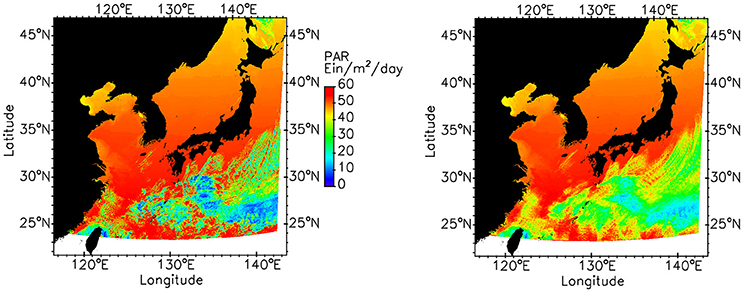
Figure 6. Daily above-surface PAR distribution for April 5, 2011 obtained from 8 hourly GOCI observations during the day (right) and a single GOCI observation at 03:16 GMT (left). In the stormy region South of Japan, the range of PAR values is smaller when using 8 observations due to diurnal changes in cloudiness. Reproduced with permission from Springer Nature (After Frouin and McPherson, 2012).

FIGURE 7

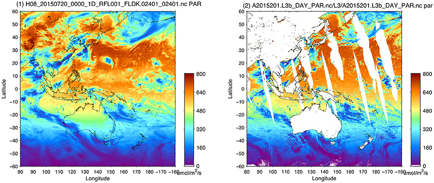
Figure 7. Daily above-surface PAR for July 20, 2011 obtained from AHI (observations every 10 min) and MODIS-A data at 9 km resolution (left and right, respectively). Patterns of spatial variability are similar for the two sensors, but the AHI PAR field is smoother, contains less extreme values, and does not exhibit spatial gaps (Courtesy of H. Murakami, Japanese Aerospace Exploration Agency).

In summary, existing satellite products generally do not cover the global open oceans (e.g., retrievals limited to Sun zenith angles <75°), except for UV irradiance, and they do not provide information below sea ice, where significant blooms may develop (e.g., Arrigo et al., 2012). In addition, cloud diurnal variability is not accounted for in daily PAR calculations when using polar orbiting satellites. Geostationary satellites observing frequently during the day account properly for cloudiness changes, but the drawback is a decreased spatial resolution at high latitudes and potentially large uncertainties for slanted viewing geometries. Propagation of surface radiation to depth currently assumes that the ocean is homogenous, neglecting potentially important effects of stratification on the absorption of solar radiation. In sum, our view of the underwater light field from space is limited. Nevertheless, the operational radiation products have been used to address a variety of topics related to aquatic photosynthesis, for example biosphere productivity during an El Niño transition (Behrenfeld et al., 2001), phytoplankton class-specific productivity (Uitz et al., 2010), chlorophyll and carbon-based ocean productivity modeling (Behrenfeld et al., 2005; Platt et al., 2008), climate-driven trends in productivity (Behrenfeld et al., 2006; Kahru et al., 2009; Henson et al., 2010), and inter-comparison of productivity algorithms (Carr et al., 2006; Lee et al., 2015). They have also been used to check the stability of CERES measurements (Loeb et al., 2006).

Users Needs

User needs vary widely in terms of products, spectral, spatial, and temporal resolution, and acceptable uncertainties, depending on the scientific or societal subject of interest. Applications requiring knowledge of radiomeric quantities and apparent properties (radiance, irradiance, average cosine, attenuation coefficients) are multiple and diverse, including phytoplankton phenology, carbon inventory, heat budget and ocean dynamics, fisheries and ecosystem management, toxic algal blooms, and eutrophication (see National Research Council, 2011 for a comprehensive list). Observational and uncertainty requirements (satellite products) generally range from 1 h to 1 day, 0.1 to 50 km, and ±5 to ±20% for PAR and 0.1 to 10 km, 1 to 7 days, and ±10 to ±25% for spectral K_d (Malenovsky and Schaepman, 2011), but higher resolution may be needed in some cases, for example rapidly changing phenomena occurring in small water bodies. For applications that need analyzing long-term records (e.g., associated with climate), the products need to be sensor independent, consistent, and continuous across satellite missions.

The satellite products should be defined unambiguously and completely, they should be easily accessible, and they should have associated ATBDs with detailed protocols including description of all ancillary data used and their sources. For example, defining a PAR product merely as downward quantum flux at the surface in the 400–700 nm spectral range is insufficient. One needs to precise whether the flux is just above or just below the surface, whether it is instantaneous or time-averaged (e.g., over 24 h for “daily PAR”), and to indicate spatial resolution. Advantages and limitations should be specified (e.g., product not valid at Sun zenith angles above 75°, or over sea ice, or in the presence of Sun glint), and uncertainties assessed, preferentially provided on a pixel-by-pixel basis, to make sure that observed changes are interpreted correctly. Computer codes used to derive the products should be available to users with proper documentation, as well as standardized processing tools (e.g., open-source toolboxes).

A survey about satellite PAR observations was conducted in 2015 by Plymouth Marine Laboratory (PML), requesting feedback from the user community on adequacy of available products, including importance, usage, and accuracy, and additional features one would like to see. Figure 8 summarizes the results about desired PAR attributes and new products and acceptable PAR uncertainties. Most respondents answered it was very or extremely important to have uncertainties associated with PAR products. About 50% of the respondents indicated that ±10–25% uncertainty was acceptable, and about 40% wanted uncertainty better than ±10%. A substantial majority of respondents ranked PAR below the surface and the fraction of PAR absorbed by phytoplankton about equally as the top two new products to generate. Based on this survey and in view of the extensive list of research and societal applications, current and potential, a list of required (new) products was compiled, including products that may be challenging to generate from space:

• Sub-surface planar and scalar irradiance (as opposed to above the surface).

• Fraction of PAR absorbed by phytoplankton (APAR).

• Diffuse fraction of total irradiance (average cosine of light field just below the surface).

• Spectral planar and scalar irradiance.

• Spectral diffuse attenuation coefficient for downward irradiance.

• Surface albedo (ratio of planar upward irradiance to downward planar irradiance just above the ocean surface).

• UV-A, UV-B scalar irradiance (with photon and energy units).

• Products without gaps (in space/time) to provide boundary conditions to models.

• Upper-ocean heating profile.

• Diurnal distribution of PAR and its attenuation.

• Averaged mixed-layer PAR.

• Under-ice light fields.

FIGURE 8

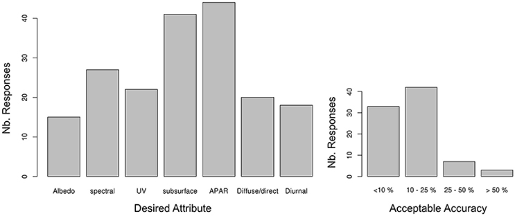
Figure 8. Results of PML user requirement questionnaire for satellite-derived PAR (Left). Histogram of desired products and attributes (Right). Histogram of acceptable uncertainty for PAR. (Based on data from 63 respondents).

Gap Analysis

Some new products (such as below surface planar and scalar PAR) can be easily implemented while others require development (e.g., APAR, vertical attenuation of PAR). For some products (e.g., under-ice light fields), the readiness level, in terms of methodology, is low. The state-of-the-art, however, is such that the strategy to obtain the new products described above is known and summarized below.

Sub-surface planar PAR and scalar PAR depend essentially on the sunlight transmission across the air-water interface, therefore the angular distribution of radiance incident at the surface and surface roughness (Mobley and Boss, 2012). The 24 h-averaged quantities, as well as the average cosine for total light, can be parameterized as a function of latitude and daily cloud factor (i.e., the ratio of actual PAR and clear-sky PAR) and wind speed. This may require look-up tables for clear sky and overcast quantities. Details about procedures are provided in section Examples of New Products, where examples of sub-surface products are presented. Note that in the OBPG approach to estimating above-surface daily planar PAR, it is actually easier (more direct) to compute the downward flux below the surface. This “penetrative” flux is obtained by subtracting from the incident extraterrestrial solar irradiance the reflected flux and the flux absorbed by the surface/atmosphere system. The “penetrative” flux is then corrected by 1/(1−A_s), where A_s is the surface albedo, to yield the incident flux onto the surface (e.g., Frouin et al., 2012). This second step introduces uncertainty, but allows for extensive evaluation at PAR measuring sites, an activity that cannot be performed easily for sub-surface fluxes (lack of data and difficulty to measure sub-surface fluxes accurately).

The above variables, integrated over the PAR spectral range, can be calculated without difficulty for the spectral bands of the ocean color sensors (i.e., visible to near infrared), in which cloud absorption is negligible. Providing the information at regular spectral intervals (e.g., every 5 or 10 nm), a requirement of some primary production models (e.g., Sathyendranath et al., 1989; Antoine et al., 1996), is straightforward since cloud optical properties (extinction coefficient, asymmetry factor) are similar, i.e., cloud albedo can be assumed constant in the entire spectral range, and the coupling between molecules and cloud droplets/crystals is relatively small (i.e., fairly unique relation between cloud transmittance at different wavelengths). In spectral regions of strong gaseous absorption, however, uncertainties may be introduced due to the coupling between absorption and scattering processes (depends on the unknown vertical distribution of the absorbers and scatterers). Extending the calculations to the ultraviolet (e.g., UV-A, UV-B) from measurements in the visible is more complicated, but definitely feasible. The complication is not due to cloud optical properties (they remain similar to those in the visible), but to the coupling between molecules and cloud droplets/crystals, which is effective. In other words, the relation between cloud transmittance (in the presence of molecules and aerosols) in the ultraviolet and visible depends on the type of clouds and their location in the vertical. This indicates that de-coupling the clear atmosphere from clouds, as it is done in the OBPG PAR algorithm, may introduce significant errors in the estimation of ultraviolet irradiance. Suitable modeling of the relation between atmospheric transmittance at visible and ultraviolet wavelengths is therefore required, which can be accomplished via radiation transfer calculations to various levels of accuracy depending on user needs (may require additional information on clouds).

From the spectral downward irradiance at the surface, minimally affected by photons reflected by the surface and backscattered by the water body (spherical albedo of the atmosphere is small, i.e., about 0.15 in the visible) and the spectral upward irradiance at the surface, one may compute the spectral surface albedo. The computation, however, can only be done in clear-sky conditions since water optical properties are necessary but generally not retrieved in cloudy conditions from ocean-color sensors. Estimating the spectral upward irradiance at the surface requires retrieving spectral water reflectance (i.e., the signal backscattered by the water body), which is routinely achieved by satellite project offices, and modeling the bidirectional reflectance function of the surface (e.g., using Cox and Munk, 1954) and the water body (e.g., using Morel and Gentili, 1996 or Park and Ruddick, 2005).

Although daily averaged quantities are often used (therefore required) in applications, instantaneous quantities (i.e., determined at time of satellite overpass) can be easily provided. In fact instantaneous products, unlike 24 h-averaged products, do not require assumptions about diurnal changes in atmospheric and oceanic properties. Diurnal variability can be described well using sensors onboard geostationary satellites, such as GOCI and AHI, see section Current Products, all the more as these sensors have ocean-color capabilities. One limitation, however, is the reduced spatial resolution at high latitudes, and managing data from different instruments, which may be operated by different space agencies, to achieve global coverage. Observations from the Earth-Sun the Lagrangian-1 (L1) point, 1.5 million kilometers from Earth, such as those made by the EPIC camera onboard DISCOVR (1–2 h temporal resolution, 21 km spatial resolution), provide a suitable alternative to several sensors on geostationary orbit. Because of the high orbit, spatial resolution at high latitudes is much less an issue. Diurnal information may also be obtained from a constellation of Sun-synchronous instruments with local overpass times spread during the day, for example MODIS-Terra at 10:30 am, SeaWiFS-SeaStar observing at noon, and MODIS-Aqua observing at 1:30 pm. From a unique instrument in Sun-synchronous orbit, ancillary data about variability of clouds and aerosols is necessary, for example Modern-Era Retrospective analysis for Research and Applications version 2 (MERRA-2) products, available at a 1/2 × 2/3 degree every hour for the day of the satellite observation.

Propagating fluxes vertically below the surface requires knowledge of the vertical profile of diffuse attenuation coefficient, K_d. From space, this can only be achieved in clear sky conditions with passive optical sensors, since K_d is deduced from water reflectance (empirical algorithms) or inherent optical properties (e.g., IOCCG, 2006). The K_d estimates are actually weighted averages over one optical depth (from which most of the photons from the water body reaching the satellite sensor originate); no vertical information is obtained. In first approximation, one may propagate light below the first optical depth (shallower than the depth of the euphotic zone) by assuming no vertical variation in spectral diffuse attenuation. However, this is generally inaccurate, as many oceanic regions (e.g., oligotrophic provinces) exhibit maximum chlorophyll concentration well below the first optical depth. One has therefore to rely on statistical relations between concentrations of oceanic constituents at the surface and below (e.g., Morel and Berthon, 1989) to estimate the K_d depth profile, or to use outputs of predictive coupled physical-biogeochemical numerical models. In the future, with the advent of space-borne polarization lidars such as CALIOP onboard CALIPSO or the Aerosol/Cloud/Ecosystems (ACE) lidar (being designed), one will be able to profile K_d in both clear and cloudy conditions, day and night, up to 3 optical depths in the green (532 nm) at a vertical resolution of 3 to 30 m (e.g., Lu et al., 2014; Behrenfeld et al., 2016). The sub-surface fluxes and the vertical profile of diffuse attenuation coefficient give access to fluxes at the bottom (important for studies of shallow coastal ecosystems), average fluxes in the mixed layer (requires knowledge of mixed-layer depth, e.g., from ocean circulation models), and the upper-ocean heating rate profile. Knowing mixed-layer fluxes and vertical heat distribution is especially useful to characterize the role of solar penetration and biological-physical interactions on ocean circulation and climate (Olhmann et al., 1996; Shell et al., 2003; see section Introduction).

In a homogeneous ocean, APAR depends on the ratio of the spectral absorption coefficient by live phytoplankton, a_ph, and total absorption (water, yellow substances, non-algal particles), a_tot, in the PAR spectral range and the spectral planar irradiance just below the surface. In a vertically heterogeneous ocean, the vertical distribution of those quantities plays a role, as well as the vertical distribution of the diffuse attenuation coefficient for downward irradiance, K_d. Computing APAR from space, therefore, requires estimates of spectral planar irradiance below the surface, and vertical profiles of a_ph, a_tot, and K_d. Sub-surface spectral irradiance and its vertical attenuation can be obtained as discussed above, and absorption coefficients using various techniques (e.g., IOCCG, 2006). Some of these variables are difficult to retrieve with good accuracy, in particular a_ph (requires partitioning a_tot into its components), and vertical information in the euphotic zone is generally not directly available (except from future space-borne lidars, see above). Consequently, uncertainties on APAR computations based on satellite estimates of individual variables may be large. Since APAR strongly depends on the spectral ratio of sub-surface reflectance, R(0⁻) and pure seawater reflectance, R_w(0⁻), one may envision approximating APAR by a linear combination of R(0⁻)/R_w(0⁻) in the PAR spectral range (Frouin et al., 2014). Since APAR is expressed linearly in water reflectance, the method is applicable to average values of water reflectance (e.g., spatially averaged), which may reduce the impact of water reflectance noise on the APAR estimate.

Primary production under sea ice is considerable, as evidenced from in situ measurements of phytoplankton concentrations and suggested by numerical model simulations. In the Arctic Ocean, it may constitute more than 30% of the total production (Popova et al., 2010). As a consequence, the seasonal cycle is shifted, with maximum primary production occurring in July, not in August-September (case of open waters). There is a need, for primary production modeling and studies of under-ice phytoplankton blooms, to determine light fields under the ice (Laliberté et al., 2016). This is quite difficult to realize from space, since knowledge of sunlight transmission though sea ice is required, and this parameter is quite variable depending on ice type and thickness, and the presence of snow and melt ponds. Transmission models are now becoming available (Arndt and Nicolaus, 2014), and they can make use of sea-ice thickness and age, snow depth, and melt pond fraction observations from microwave and optical sensors (SIRAL on Cryosat-2, AMSR-2 on CGOM-W1, ATLAS on IceSta-2, MODIS on Terra and Aqua). One issue is separating the contribution of clouds to the planetary albedo, in order to access the surface albedo. Algorithms are not mature for generating operationally shortwave fluxes under sea ice.

The possible methodologies, difficulties, opportunities, and readiness level for developing and creating the new products were discussed above. The following recommendations regarding these products are made:

1) Spectral fields should be provided at the sensor resolution with protocols (and codes) describing how to interpolate and extrapolate for obtaining other spectral distributions (e.g., 1 nm irradiance field from a multi-spectral sensor).

2) Vertical propagation of products requires an appropriate attenuation coefficient from which other products can be derived (e.g., euphotic depth, mixed-layer depth, isolume depth). Clear guidelines on how to produce the derived products using the attenuation should be provided.

3) Horizontal/temporal gap filling is necessary for certain applications (e.g., ecological forecasting). This can be done using merged products across sensors and/or interpolation schemes (using known de-correlation scales or models). Many techniques are available (e.g., Pottier et al., 2006; Alvera-Azcarate et al., 2007; Krasnopolsk et al., 2016).

4) Products should have associated uncertainties that are consistent with those obtained when validating estimates against in situ measurements, taking into account uncertainties in the in situ data. This requires a calibration/validation program. The product protocol should provide a description of how the uncertainty was derived. It is desirable to provide a per-pixel uncertainty. It is recognized that the level of effort to obtain a very accurate uncertainty estimate can be very large and therefore some trade-offs may need to be done, in consultation with user requirements.

5) Data access should be tailored to users need. For example, modelers will use multithreading with simultaneous access to associated error fields. In contrast, the Earth observation community will, typically, want to access data using FTP. Most users do not care about the satellite mission from which a product was derived, but rather care about the products being continuous in time and consistent across missions.

6) Cross-agency efforts should be made to homogenize their respective products so it is easy for users to use these products (e.g., the definition of a PAR product should be the same). For climate relevant products, it is critical to merge them (and de-bias) across missions so that models to not experience secular jumps as they assimilate such data.

Examples of New Products

Par Simulator

Radiative Transfer Code

To develop new shortwave radiation products from satellite data (such as those discussed above) and assess accuracies, one needs to simulate the TOA radiance measured by a given sensor and the variable to retrieve (e.g., planar or scalar spectral irradiance below the surface, average cosine). For this, we use the Speed up Monte-Carlo Advanced Radiative Transfer using GPU (SMART-G) radiative transfer code (Ramon et al., 2017). This code, based on the Monte-Carlo method, is fast and massively parallel. It computes the complete light field (i.e., radiance, including polarization) in the ocean and atmosphere.

The code simulates the transfer/propagation of solar radiation in a 1-dimensional coupled ocean-atmosphere system with a wavy interface. It accounts for absorption and scattering by molecules, aerosols, and hydrosols, and Fresnel reflection/refraction at the interface. Polarization properties of the various atmospheric and oceanic constituents and the surface are explicitly considered. Inelastic processes (i.e., Raman scattering, fluorescence) are omitted in the current version. The ocean can be infinitely deep or bounded by a reflective bottom at finite depth. The computations are made in either plane-parallel or spherical geometry. The four components of the Stokes vector can be obtained at any wavelength of the solar spectrum and any level of the coupled ocean-atmosphere system.

Gaseous absorption is treated either by correlated k-distribution (Kato et al., 1999) or an equivalent like REPTRAN (Gasteiger et al., 2014; Emde et al., 2016). In the multispectral mode, each photon is assigned a wavelength. All optical properties of the medium are pre-calculated for these wavelengths. The spectrum is computed in one pass but is under the influence of Monte-Carlo noise. For higher spectral resolution computations without spectral noise, for example in order to handle line-by-line (LBL) gas absorption, the ALIS method (Emde et al., 2011) is also implemented in SMART-G. This allows for the calculation of spectra by tracing the photon paths once for all wavelengths (by absorption/scattering decoupling).

Simulations

In the Monte-Carlo code, photon packets are carrying planar irradiance (Wm⁻²) perpendicular to their direction of propagation. Therefore downward or upward spectral planar irradiances are obtained by performing the weighted sum of irradiances crossing a unit area of horizontal surface located above or below the air-sea interface. For spherical irradiances, each photon is assigned an additional weight of 1/cos(θ_i) where θ_i is the photon's zenith angle arriving on the detector. The runs were optimized for the calculation of spectral daily fluxes above and below the ocean surface. For 1 day, one run was executed by injecting a large number of photons whose wavelength was chosen randomly as well as the injection angles at TOA and in the atmosphere depending on the hour of the day. Typical runtime is 1 s to reach ±1% uncertainty for clear sky conditions and for 1 day. It becomes 30 s for a totally overcast situation with a cloud optical thickness of 50.

The aerosol and cloud optical properties are taken from the OPAC database (Hess et al., 1998) and distributed within the libradtran software package (www.libradtran.org). Aerosols are supposed to be spherical. The clouds are supposed to be composed of liquid water droplets with a varying effective radius. Rayleigh optical depth is computed according to Bodhaine et al. (1999). The gaseous absorption is parameterized as a correlated k-distribution with spectral intervals of 10 nm from line-by-line calculations using the Py4Cats code (Schreier and Gimeno Garcia, 2013) and HITRAN 2012 (Rothman et al., 2013) absorption parameters for H₂O and O₂. Ozone and NO₂ smooth absorption coefficient are taken from Bogumil et al. (2003). The wind-roughened sea surface is modeled as an ensemble of uncorrelated facets with a slope distribution (Cox and Munk, 1954) and a uniform azimuth distribution. The reflection and transmission coefficients are then computed using Fresnel's laws. Ocean bulk optical properties correspond to Case-I waters with a chlorophyll-a concentration of 0.5 g.m⁻³. The ocean's bottom is black and is located at a depth of 50 m. The ocean phase function is represented by a Fournier-Forand function with a varying truncation angle.

An example of outputs of the SMART-G code in the context of PAR simulations (both spectral irradiance and reflectance) is given in Figure 9 for various levels in the atmosphere-ocean system (top, just above the surface, just below the surface, and at the black bottom of the water column) and several atmospheric conditions (clear and cloudy situations with different Sun zenith angles). The TOA reflectance in the MERIS bands is also indicated. The various graphs show the importance of Sun zenith angle and cloud optical thickness in controlling the downward PAR above and below the surface. They also illustrate the usefulness of the SMART-G tool for algorithm development.

FIGURE 9

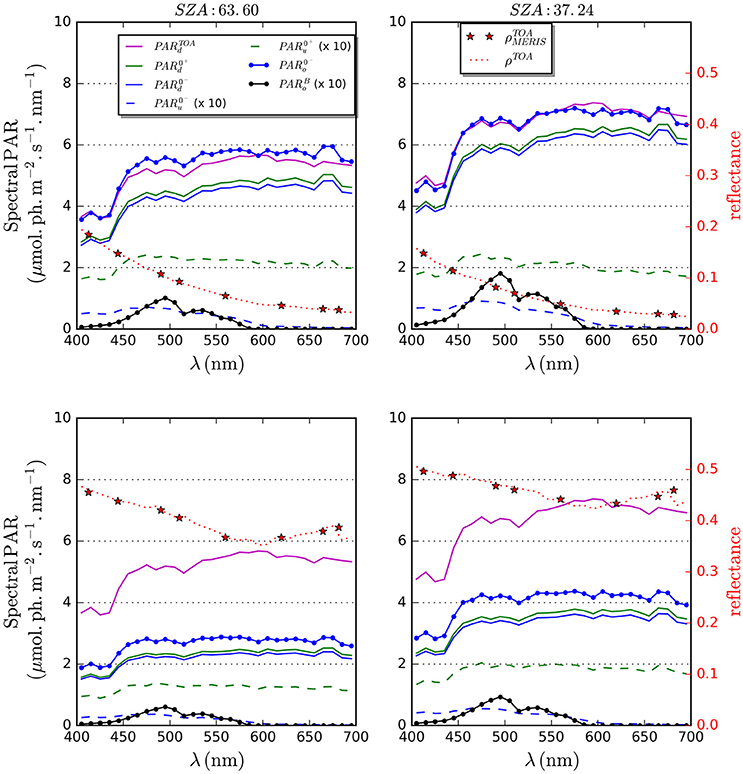
Figure 9. Examples of outputs of the SMART-G RTC code for 4 situations. On the left axis is reported the “spectral PAR” in units of light quanta per unit time, unit area and unit wavelength for planar and spherical upwelling (“u”) or downwelling irradiances (“d”) at several levels in the ocean-atmosphere coupled system: at TOA, just above (0⁺) or below (0⁻) the surface, or at the black bottom (superscript B) of the ocean located here at a depth of 50 m. On the right axis is plotted the TOA spectral reflectance at the same resolution, and at the center of MERIS wavebands. The top two graphs are for a clear-sky situation for two Sun zenith angles (SZA) and the bottom two graphs a liquid water cloud, located between 2 and 4 km with droplets of effective radius = 11 mm whose of optical thickness 10 is added. The clear atmosphere model is the US62 standard atmosphere, with maritime polluted aerosols as described in the OPAC database with an AOT at 550 nm equal to 0.1. The ozone column is 300 DU and the precipitable water quantity is 2 g/cm².

For the year 2011, and for 14 latitudes ranging from −64.5 to 64.5, the various spectral irradiances listed in the Annex were computed at 11 times regularly distributed throughout the day. The typical spectral TOA reflectance for a MERIS-like instrument measuring at 10:30 local time was also computed. The atmospheric content was changing according to the MERRA-2, hourly, gridded datasets of water vapor and ozone contents, aerosol optical depths of black carbon, dust, organic carbon, sea salt, and sulfates aerosols at 550 nm, and cloud optical thicknesses. Individual clear sky and overcast plane-parallel radiative transfer calculations were then mixed using the Independent Pixel Approximation (IPA) using MERRA-2 cloud cover variable as the mixing value.

The following quantities were then computed: $PA{R}_o^{0-}(t)$ $\text{and }{PAR}_d^{0+}(t)$ (to describe diurnal variation of sub-surface fluxes), ${\langle PA{R}_d^{0+}\rangle }_{24h}$ (the main product), ${\langle PA{R}_o^{0-}\rangle }_{24h}$ (the key product for primary production and photo-chemical processes), ${\langle PA{R}_o^{0-}\rangle }_{24h}({\lambda }_i)$ (spectral scalar flux, as requested by modelers, at a resolution of 10 nm), and ${\langle {\mu }_0^{0-}\rangle }_{24h}$(to characterize the angular structure of the light field). Definitions are provided in the Annex.

Algorithm for ${\langle {\text{PAR}}_{\text{o}}^{0+}\rangle }_{24\text{h}}$ and ${\langle {\mu }_0^{0-}\rangle }_{24\text{h}}$

Rationale

We define a Cloud Factor (CF) as the deviation from a pure clear sky daily averaged PAR above the surface. It is a “measure” of the influence of clouds on the daily PAR:

${\langle CF\rangle }_{24h}=\frac{{\langle PA{R}_d^{0+}\rangle }_{24h}}{{\langle PA{R}_d^{0+}\rangle }_{24h}^{clear}}$

One typical day of simulations is displayed in Figure 10 for a latitude of 55.5°N. The Sun zenith angle and the length of the day mainly drive the diurnal cycle of both clear sky PAR and partly cloudy PAR. For that particular day, the influence of cloudiness is important (and somehow stable) reducing the daily PAR by a factor 〈CF〉_24h = 0.34. The average cosine ${\mu }_0^{0-}$is very stable for cloudy conditions, with a value around 0.82 throughout the day. A clear sky has a variable ${\mu }_0^{0-}$ culminating at noon. In both cases the spectral variation of${\mu }_0^{0-}$, not shown here, is weak. The 24 h-averaged value of${\mu }_0^{0-}$should be representative of the direction of propagation of the largest fraction of the daily PAR. That is why we define the 24 h-averaged ${\langle {\mu }_0^{0-}\rangle }_{24h}$ as the ratio of the 24 h-averaged net and scalar PAR (and not the 24 h average of their instantaneous ratios):

${\langle {\mu }_0^{0-}\rangle }_{24h}=\frac{{\langle E_{net}^{0-}\rangle }_{24h}}{{\langle E_o^{0-}\rangle }_{24h}}$

FIGURE 10

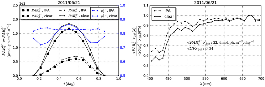
Figure 10. (Left plot) Diurnal variation of the downward above-surface PAR (squares) and scalar below-surface PAR (dots) for the 21st of June and for a latitude of 55.5° N and a wind speed of 0 m/s. On the right vertical axis is reported the mean cosine below the surface. Two simulations are shown: (i) one for clear sky (solid lines) and (ii) one for “real” sky with cloud cover and cloud optical thickness as given by MERRA-2 and mixed with the clear-sky simulations using the Independent Pixel Approximation (IPA). (Right plot) Normalized spectral PAR at 675 nm for both clear and IPA situations.

The normalized spectral PAR, obtained by dividing the spectral PAR by its value at 675 nm, is defined in the same manner as:

${\langle P\widetilde{A{R}_o^{0-}}\rangle }_{24h}\left({\lambda }_i\right)=\frac{{\langle PA{R}_o^{0-}\rangle }_{24h}\left({\lambda }_i\right)}{{\langle PA{R}_o^{0-}\rangle }_{24h}\left(675\text{nm}\right)}$

It gives the spectral shape of the PAR and it is very stable and close to the TOA solar irradiance spectrum in most cases. The spectral shape of the clear sky PAR is slightly influenced by the mean Sun zenith angle because the absorption of ozone in Chappuis bands becomes more and more effective. The spectral dependence of the cloudy PAR is smaller. It increases in the blue part of the spectrum as cloud influence increases.

Following the approach of Mobley and Boss (2012), 24 h-averaged secondary radiative quantities may be obtained from a reduced set of parameters, the most important ones being the location and date which control the day length and mean Sun zenith angle, then the influence of the clouds which is between null (clear sky) and maximum (100% cloud cover), and finally the wind speed. The chlorophyll content of the water is of minor importance for calculating the scalar and net PAR just below the surface. Figure 11 displays the coefficients to be applied to ${\langle PA{R}_d^{0+}\rangle }_{24h}$ in order to obtain ${\langle PA{R}_o^{0-}\rangle }_{24h}$, or ${\langle PA{R}_d^{0-}\rangle }_{24h}$, and also shows how ${\langle {\mu }_0^{0-}\rangle }_{24h}$ and ${\langle P\widetilde{A{R}_o^{0-}}\rangle }_{24h}({\lambda }_i)$ vary for various latitudes and wind speeds and for the two extreme cases, i.e., clear and totally overcast. Figure 12 displays the result of the application of the coefficients described above for estimating the scalar PAR below the surface. We processed one full year of global simulated data (2011, see section PAR Simulator) for 3 wind speeds (0, 7, and 15 m.s⁻¹) and checked the quality of the regression vs. the “actual” (or prescribed) values, i.e., the values obtained by running the Monte Carlo code with the various input variables (MERRA-2 hourly data, see above). These values provide the reference in calculating algorithm performance statistics. The regression is excellent with a residual bias and a R.M.S. difference of about 0.5 mol.ph m⁻².day⁻¹. Wind speed or cloudiness do not apparently impact the quality of the regression.

FIGURE 11

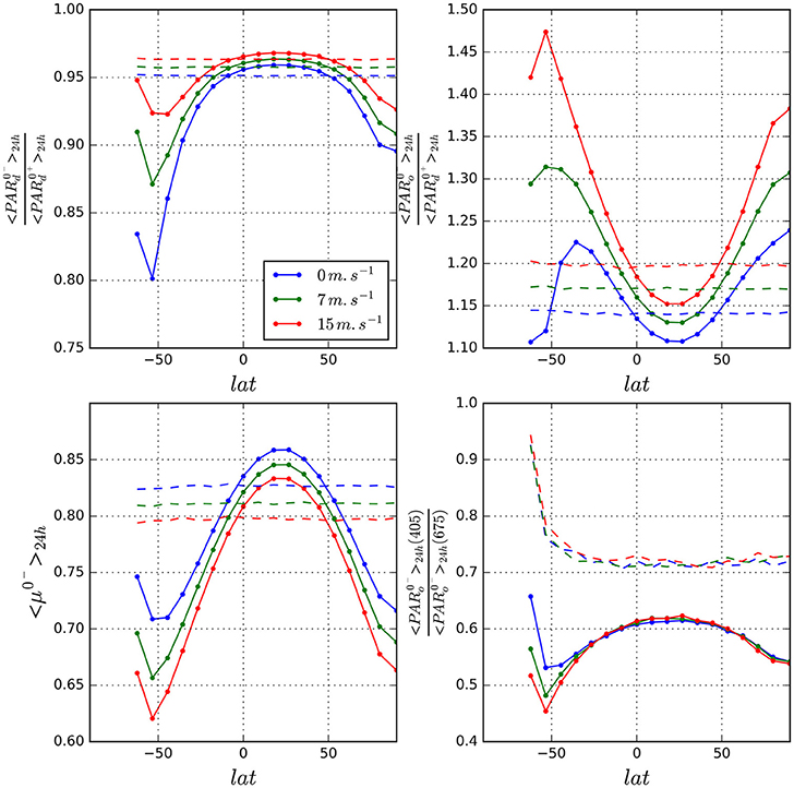
Figure 11. Simulations of 24 h averaged secondary radiative products for clear-sky (solid lines) and totally overcast situations (dashed lines, cloud optical thickness = 50, constant along the day) and for several wind speed as a function of latitude. (Top left) Ratio of planar PAR below and above surface. (Top right) Ratio of scalar PAR below the surface to planar PAR above surface. (Bottom left) Average cosine below the surface. (Bottom right) Ratio of spectral scalar PAR below the surface at 405 and 765 nm. The date is 21st of June.

FIGURE 12

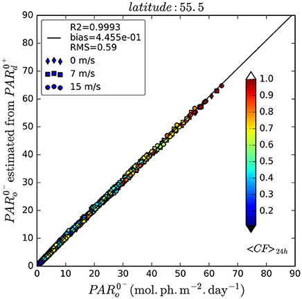
Figure 12. Estimated scalar PAR below the surface from the planar PAR above surface and the clear sky “transmission factors” shown in Figure 11 for all the days of 2011 and 3 wind speeds. The color of the symbols is a function of the cloud factor.

Figures 13, 14 depict the normalized spectral PAR and average cosine for the year 2011, for a latitude of 55.5°N and a wind speed of 7 m.s⁻¹. For both parameters, the clear sky and totally overcast situations are also plotted. They constitute an envelope wihin which the actual values are included, and the deviation from the clear sky value seems proportional to the actual cloud factor 〈CF〉_24h. This suggests a method to derive ${\langle P\widetilde{A{R}_o^{0-}}\rangle }_{24h}({\lambda }_i)$ and ${\langle {\mu }_0^{0-}\rangle }_{24h}$ from look-up tables of the clear sky and overcast situations and from an estimation of the actual cloud factor.

FIGURE 13

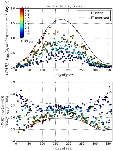
Figure 13. (Top) Scalar PAR below the surface integrated in a narrow spectral band (400–410 nm) for all the days of 2011 (dots), for a particular latitude and wind speed, as well as predicted values for clear sky (solid line) and totally overcast situations (dashed lines). (Bottom) Same as top but normalized by the band integrated scalar PAR below the surface between 670 and 680 nm. The color of the dots is a function of the cloud factor.

FIGURE 14

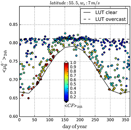
Figure 14. Mean cosine PAR for all the days of 2011 (dots), for a particular latitude and wind speed, as well as predicted values for clear sky (solid line) and totally overcast situations (dashed lines). The color of the dots is a function of the cloud factor.

Equations

We propose to use the observed cloud factor 〈CF〉^obs as a proxy of 〈CF〉_24h and then linearly interpolate between clear sky and overcast look-up tables as a function of 〈CF〉^obs. We have:

$\begin{array}{l}{\langle \text{CF}\rangle }^{\text{obs}}=\frac{{\langle {\text{PAR}}_{\text{d}}^{0+}\rangle }_{24h}^{\text{obs}}}{{\langle {\text{PAR}}_{\text{d}}^{0+}\rangle }_{24h}^{\text{clear}}}\\ S1=\frac{{\langle P\widetilde{A{R}_o^{0-}}\rangle }_{24h}^{\text{clear}}\left({\lambda }_i\right)-{\langle P\widetilde{A{R}_o^{0-}}\rangle }_{24h}^{\text{overcast}}\left({\lambda }_i\right)}{1-{\langle CF\rangle }_{24h}^{\text{overcast}}}\\ {\langle P\widetilde{A{R}_o^{0-}}\rangle }_{24h}\left({\lambda }_i\right)=S1.\left({\langle CF\rangle }^{obs}-{\langle CF\rangle }_{24h}^{overcast}\right)\\ +{\langle P\widetilde{A{R}_o^{0-}}\rangle }_{24h}^{\text{overcast}}\left({\lambda }_i\right)\\ S2=\frac{{\langle {\mu }_0^{0-}\rangle }_{24h}^{\text{clear}}-{\langle {\mu }_0^{0-}\rangle }_{24h}^{\text{overcast}}}{1-{\langle CF\rangle }_{24h}^{overcast}}\\ {\langle {\mu }_0^{0-}\rangle }_{24h}=S2.\left({\langle CF\rangle }^{obs}-{\langle CF\rangle }_{24h}^{\text{overcast}}\right)+{\langle {\mu }_0^{0-}\rangle }_{24h}^{\text{overcast}}\end{array}$

The error will be large when cloudiness changes a lot during the day and thus we may suspect that 〈CF〉^obs deviates substantially from 〈CF〉_24h and when the values of the parameters in clear or totally cloudy conditions are substantially different.

Look- Up Tables for Clear Sky and Overcast Situations

Models

The clear sky model is based on the AFGL US 62 standard atmosphere with a surface pressure of 1012.15 hPa, an O₃ vertically integrated content of 300 DU, and a H₂O vertically integrated content of 2 g.cm⁻². The aerosol model is the maritime clean model from the OPAC database with an AOT of 0.1 at 550 nm. The air-sea interface is a wind-roughened surface. The ocean bulk optical properties correspond to Case-I waters with a chlorophyll a concentration of 0.5 g.m⁻³. The ocean bottom is black and is located at a depth of 50 m. For the totally overcast model we added a permanent cloud layer between 5 and 10 km consisting of water droplets with r_eff = 11 μm and a cloud optical thickness of 50. The aerosols, hydrosols and cloud phase matrices are computed at 550 nm and are assumed spectrally invariant between 400 and 700 nm.

Computations

For latitudes between −90° and 90° by step of 10°, for every 30 days along the year, and for 3 wind speeds: 0, 7 and 15 m.s⁻¹, we computed the following quantities:

$\begin{array}{l}{\langle CF\rangle }_{24h}^{\text{overcast}},{\langle P\widetilde{A{R}_o^{0-}}\rangle }_{24h}^{\text{overcast}}({\lambda }_i),{\langle P\widetilde{A{R}_o^{0-}}\rangle }_{24h}^{\text{clear}}({\lambda }_i),{\langle {\mu }_0^{0-}\rangle }_{24h}^{\text{overcast}},\hfill \\ and{\langle {\mu }_0^{0-}\rangle }_{24h}^{\text{clear}}\hfill \end{array}$

First Results

For the MERIS sensor, first examples of the new parameters (daily and monthly global products for May 15 and May 1–31, 2011) are displayed in Figures 15–17. Data at high latitudes were masked using ESA CCI Sea Ice Concentration products v2.0 (cci.esa.int). The scalar PAR below the surface (Figure 15) follows the planar PAR above the surface (not shown here), but the values are somewhat higher, as expected. The spatial coverage of the daily MERIS product is less than for the MODIS products (Figure 1), because of the narrower swath of MERIS and the glitter mask (more glint in the MERIS imagery). The average cosine product (Figure 16) is smoother because it is influenced mainly by the average solar elevation. The latitudinal variation is important with the highest values (0.85) in the tropics whatever the cloudiness. At high latitudes the contrast between clear and cloudy sky conditions becomes more marked with an average cosine closer to the tropics values in cloudy sky conditions and the lowest values (0.65) under clear skies. For monthly averages, the mixture between cloudy and clear skies tends to further smooth the product, which becomes a simple function of latitude. The normalized spectral PAR at 405 nm (Figure 17), like the mean cosine, exhibits a contrast between clear and cloudy sky situations that is increasing toward the high latitudes. However on a monthly time scale the latitudinal gradient is very weak and the dispersion of the product is also very weak with a mean of 0.63 and a standard deviation of 0.024 over the global ocean.

FIGURE 15

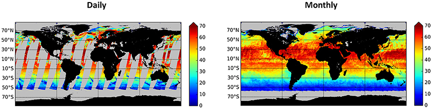
Figure 15. Daily, and monthly scalar PAR below surface (unit: E/m²/day), 0.1° spatial resolution derived from MERIS. Top Left: May 15, 2011; Top Right: May 1–31, 2011.

FIGURE 16

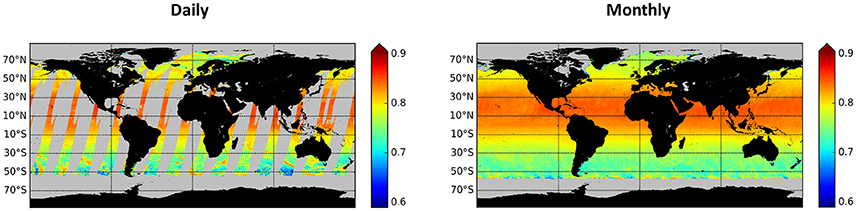
Figure 16. Same as Figure 15 but for the average cosine below the surface.

FIGURE 17

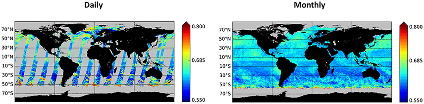
Figure 17. Same as Figure 15 but for the ratio of spectral scalar PAR below the surface at 405 and 675 nm.

Algorithm Uncertainties for ${\langle {PAR}_d^{0+}\rangle }_{24h}$

Associating uncertainties to the satellite radiation products, preferentially on a pixel-by-pixel basis, is obligatory to quantify their quality. This is important to ensure that variability or trends detected in scientific analyses are of geophysical nature, i.e., that the data are interpreted properly in view of their strengths and limitations, and to merge different data sets. This is also essential for data assimilation, a primary application of the products (large uncertainties will have little impact on model runs, small uncertainties will constrain the model to behave like the data). Expressing uncertainties requires modeling the measurement, identifying all possible error sources (e.g., noise in the input variables, imperfect/incomplete mathematical model), and determining the combined uncertainty, as described in JGCM-100 (2008) and subsequent publications.

In the following, algorithm uncertainties associated with ${\langle PA{R}_d^{0+}\rangle }_{24h}$ are considered, i.e., those due to model approximations and parameter errors (e.g., decoupling effects of clouds and clear atmosphere, neglecting diurnal variability of clouds, using aerosol climatology) assuming that the input variables (TOA reflectance at wavelengths in the PAR spectral range) are known perfectly. A procedure is provided to estimate and provide, for each pixel of a product, this uncertainty component of the total uncertainty budget, which is expected to dominate. The uncertainty characterization has been done using an extended simulation dataset covering the 2003–2012 time period still using 1 hourly MERRA-2 input data. The large number of data points allows one to sample well the atmospheric variability and in particular many variations of daytime nebulosity, for all latitudes.

Figure 18 displays the result of the uncertainty analysis for the whole dataset. The bias and the standard deviation of the daily PAR estimates are plotted as a function of the clear-sky PAR (which depends itself mainly on latitude and date) and the actual cloud factor for that day. The Monte Carlo calculations, assumed accurate, provide the reference. This is justified in view of the bias and standard deviation values. The bias exhibits a slight dependence on the clear sky PAR, suggesting an overestimation reaching 2.5 E.m⁻².day⁻¹ (~4%) for the maximum clear sky PAR values, and a slight underestimation 1 E.m⁻².day⁻¹ (~6.5%) when the clear sky PAR reaches a low value of 15 E.m⁻².day⁻¹. When looking at the dependence upon 〈CF〉_24h, a slight overestimation exists between 1 and 1.5 E.m⁻².day⁻¹. This overestimation is independent of the cloudiness of the day, with the exception of totally clear days (〈CF〉_24h = 1), for which the bias drops to 0.5 E.m⁻².day⁻¹. The bias is also quite small for totally overcast situations. A bias correction can be considered, based on the clear-sky PAR value.

FIGURE 18

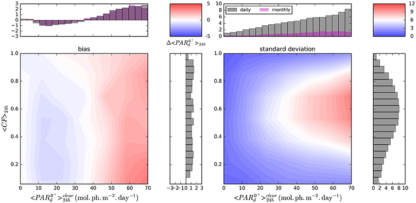
Figure 18. Error budget of the daily “MERIS” PAR product above the surface (estimated PAR–actual PAR) from simulations for the period 2003–2012 using 1-hourly resolved MERRA-2 input data. For each day, a set of MERIS spectral reflectance data is simulated for a typical observation at 10:30 UT local time and several viewing geometries (nadir and 20° view zenith angle (VZA) with relative azimuth of 0, 90, and 180°, with sun glint avoidance). (Left) 2D plot of the error bias as a function of the clear sky daily PAR above surface (x axis) and cloud factor (y axis), along with 1D (marginal) distribution. (Right) Same as left but for the error standard deviation. For the 1D marginal distribution as a function of the clear-sky PAR is also reported the monthly PAR error bias and standard deviation in magenta.

The standard deviation (SD) is peaked toward intermediate cloud factors, where the risk of deviation of cloudiness at the time of the satellite measurement and the mean cloudiness of the day is maximum. When the clear sky PAR is large and 〈CF〉_24h is about 0.5, SD reaches 8 E.m⁻².day⁻¹ (~11%). But SD drops to 1 E.m⁻².day⁻¹ (1.5%) for clear sky situations (〈CF〉_24h = 1). SD is drastically reduced when dealing with monthly PAR estimates. Whatever the cloudiness, SD is lower than 2 E.m⁻².day⁻¹. The main feature is that SD seems to be proportional to the clear-sky PAR value, and thus we can consider associating an uncertainty to each pixel of the product from an estimate of the clear-sky value, in addition to the cloud factor. This model uncertainty component could be extended to situations with multiple satellite measurements per day, as it is often the case for high latitudes with polar orbiting sensors like MERIS or VIIRS. In that case we anticipate a reduction of the standard deviation of the daily PAR product. For a complete per-pixel uncertainty budget, the uncertainty associated with TOA reflectance noise (radiometric and due to vicarious calibration) should be included, which may require evaluating the sensitivity of the daily PAR to the TOA reflectance and the covariance of the input reflectance in the various spectral bands (since the measurements are correlated).

Summary and Recommendations

Studying and understanding the chemical, physical, geological, and biological processes that govern the composition of the marine environment requires knowledge of the underwater light field. Ideally, one wants to figure out and monitor the spectral and angular structure of the radiant intensity at any point in the water body. From space, by means of remote sensing, only limited information about the radiative properties of a water body can be obtained, but the advantage is global and repetitive coverage. Existing satellite products are restricted to planar PAR and UV irradiance above the surface, and diffuse attenuation coefficient (average in the upper layer). These products, despite their drawbacks (e.g., no information at high Sun zenith angles and diurnal variability poorly described for PAR, no retrieval in cloudy conditions for the diffuse attenuation coefficient), have been useful to many studies of aquatic photosynthesis, heat budget, and chemical effects of light. There is a need, however, for other products, i.e., sub-surface planar and scalar fluxes, average cosine, spectral fluxes (UV to visible), diurnal fluxes, APAR, surface albedo, vertical attenuation, and heating rate, and for associating uncertainties to any product on a pixel-by-pixel basis. Possible approaches and methodologies to generate these new products, in view of state-of-the-art knowledge and current and planned satellite missions, were discussed, including difficulties, assumptions, and readiness level. A strategy and a roadmap, with development priorities and opportunities to obtain the new products, could be established. Examples of new products, i.e., daily scalar PAR below the surface, daily average cosine for PAR, and spectral scalar fluxes below the surface, and their algorithms, were presented. A statistical way to estimate uncertainties for each pixel, based on radiative transfer simulations for expected clear and cloudy situations, was proposed.

In the short term, the focus should be on improving/completing existing products from satellite ocean-color sensors, i.e., extending calculations of above-surface fluxes to high Sun zenith angles and accounting, at least statistically, for diurnal variability of clouds. One should also work on how to compute similar products from different missions and their likely uncertainties, to obtain platform-independent global products. On the other hand, with existing scientific knowledge, the following new products (see sections Current Products and Users Needs) should be derived from past and current missions: planar and scalar PAR below the surface, average cosine for PAR below the surface, diffuse attenuation coefficient for PAR, and respective spectral quantities (visible to near infrared), spectral albedo, and APAR. These products should be in the form of daily averages, except for diffuse attenuation coefficient. New processing lines will require links with other ocean and atmosphere products and/or ancillary data (e.g., reanalysis products from observations and models, such as MERRA-2). A calibration/validation program should be planned to evaluate the new products and their uncertainty over a representative set of conditions.

In the medium term (longer-term effort, not lower priority), with specific efforts and new avenues in algorithm development, the aim should be to generate the following products, not only from past and current missions, but also from future missions: spectral fluxes below the surface and diffuse attenuation in the UV (or integrated over UV-A and UV-B ranges), in both photon and energy units, especially using TROPOMI on Sentinel 5P/5, average mixed-layer PAR (will require mixed-layer depth fields from Argo-assimilated circulation models), upper-ocean heating profile, and under-ice light fields (in conjunction with cryosphere missions and modeling). Diurnal-cycle resolving measurements, combining different satellites over-passing at different times with geostationary satellites, should be pursued to describe hourly changes in radiation fields and improve daily-integrated values (e.g., due to clouds). The products should also be generated without gaps (applying gap-filling techniques) to provide boundary conditions for general circulation models. At this stage, evaluation of the products and their uncertainty should be ongoing on a continuous basis.

In the long term (future vision), for significant improvement of sub-surface light fields, space lidars could be used (e.g., the CNES MESCAL), as they can resolve the vertical distribution of material in the ocean (while all the products described above, derived from passive optical sensors, assume a homogeneous upper ocean). This is particularly critical in high-latitude regions (near the ice) and near land. Approaches using hyper-spectrally resolved sensors such as SCHIMACHY to retrieve the availability of light in the ocean (depth-integrated scalar irradiance) from the vibrational Raman scattering effect of water molecules (Dinter et al., 2015) should be explored. Finally, satellites missions with instruments in L1 orbit (such as the NASA EPIC onboard DISCOVR) would offer the opportunity to continuously observe the sun-lit part of the ocean, maximizing the temporal coverage. Space agencies should consider exploiting using such orbit for an ocean-color satellite mission.

Author Contributions

All the authors contributed to the conception and organization of the study, to the analysis of the various products and results, and to the writing of the findings. RF, DR, and EB arranged the contents of the various sections, and wrote the first version of the manuscript. HB provided insight into light and biogeochemical processes. JT and BF carried out the work related to current MODIS and OMI products. DR, DJ, MC, and RF developed algorithms for new products and devised ways to associate uncertainties. DR, DJ, and MC generated examples of new products. TJ, TP, and SS organized the survey about satellite PAR observations and compiled and synthesized user responses. All the authors critically revised the manuscript and helped to bring about its final version.

Funding

The National Aeronautics and Space Administration (NASA) and the European Space Agency (ESA) provided funding for the study under Grant NNX14AL91G and Contract 40001 1 3690/1 4/I-LG, respectively.

Conflict of Interest Statement

The authors declare that the research was conducted in the absence of any commercial or financial relationships that could be construed as a potential conflict of interest.

Acknowledgments

The authors gratefully acknowledge the NASA Ocean Biology Processing Group (OBPG) and the OMI Science Investigator-led Processing System (SIPS) Facility at Goddard Space Flight center, Greenbelt, Maryland for generating and maintaining ocean-color and radiation products used in the study, and Mr. John McPherson, from Scripps Institution of Oceanography and Mr. Monstreleet and Mr. Laurent Wandrebeck from HYGEOS for providing technical support. The survey about PAR products, which involved human participants, did not require ethics approval as per institutional and national guidelines. The participants consented to release the results by virtue of survey completion.

References

Alvera-Azcarate, A., Barth, J.-H., Beckers, M., and Weisberg, R. (2007). Multivariate reconstruction of missing data in sea surface temperature, chlorophyll, and wind satellite fields. J. Geophys. Res. 112:C03008. doi: 10.1029/2006JC003660

CrossRef Full Text | Google Scholar

Antoine, D., André, J. M., and Morel, A. (1996). Oceanic primary production: 2. Estimation at global scale from satellite (coastal zone color scanner) chlorophyll, Glob. Biogeochem. Cycles 10, 57–69. doi: 10.1029/95GB02832

CrossRef Full Text | Google Scholar

Arndt, S., and Nicolaus, M. (2014). Seasonal cycle and long-term trend of solar energy fluxes through Arctic sea ice. Cryosphere 8, 2219–2233, doi: 10.5194/tc-8-2219-2014

CrossRef Full Text | Google Scholar

Arola, A., Kazadzis, S., Lindfors, A., Krotkov, N., Kujanpää, J., Tamminen, J, et al. (2009). A new approach to correct for absorbing aerosols in OMI UV. Geophys. Res. Lett. 36:L22805, doi: 10.1029/2009GL041137

CrossRef Full Text | Google Scholar

Arrigo, K. R., Perovich, D. K., Pickart, R. S., Brown, Z. W., van Dijken, G. L., et al. (2012). Massive phytoplankton blooms under Arctic sea ice. Science 336:1408. doi: 10.1126/science.1215065

PubMed Abstract | CrossRef Full Text | Google Scholar

Ballabrera-Poy, J., Murtugudde, R., Zhang, R.-H., and Busalacchi, A. J. (2007). Coupled ocean–atmosphere response to seasonal modulation of ocean color: impact on interannual climate simulations in the Tropical Pacific. Am. Meteorol. Soc. 20, 353–374. doi: 10.1175/JCLI3958.1

CrossRef Full Text | Google Scholar

Behrenfeld, M., Hostetler, C., Sarmiento, J., in collaboration with the, N. A. S. A., Ocean Biology Biogeochemistry Advance Planning Committee (2016). A Global Ocean Science Target for the Coming Decade. Washington, DC: Response to the 2017 NRC Decadal Survey Request for Information.

Google Scholar

Behrenfeld, M. J., O'Malley, R. T., Siegel, D. A., McClain, C. R., Sarmiento, J. L., Feldman, G. C., et al. (2006). Climate-driven trends in contemporary ocean productivity. Nature 444, 752–755. doi: 10.1038/nature05317

PubMed Abstract | CrossRef Full Text | Google Scholar

Behrenfeld, M. J., Boss, E., Siegel, D. A., and Shea, D. M. (2005). Carbon-based ocean productivity and phytoplankton physiology from space. Glob. Biogeochem. Cycles 19:GB1006. doi: 10.1029/2004GB002299

CrossRef Full Text | Google Scholar

Behrenfeld, M. J., Randerson, J., McClain, C., Feldman, G., Los, S., Tucker, C., et al. (2001). Biospheric primary production during an ENSO transition. Science 291, 2594–2597. doi: 10.1126/science.1055071

PubMed Abstract | CrossRef Full Text | Google Scholar

Bodhaine, B. A., Wood, N. B., Dutton, E. G., and Slusser, J. R. (1999). On Rayleigh optical depth calculations. J. Atmos. Oceanic Tech. 16, 1854–1861.

Bogumil, K., Orphal, J., Homann, T., Voigt, S., Spietz, P., Fleischmann, O. C., et al. (2003). Measurements of molecular absorption spectra with the SCIAMACHY pre-flight model: instrument characterization and reference data for atmospheric remote sensing in the 230–2380 nm region. J. Photochem. Photobio. 157, 167–184. doi: 10.1016/S1010-6030(03)00062-5

CrossRef Full Text | Google Scholar

Carr, M.-E., Friedrichs, M. A. M., Schmeltz, M., Noguchi Aita, M., Antoine, D., Arrigo, K. R., et al. (2006). A comparison of global estimates of marine primary production from ocean color. Deep Sea Res. II 53, 741–770. doi: 10.1016/j.dsr2.2006.01.028

CrossRef Full Text | Google Scholar

Cox, C., and Munk, W. (1954). Measurement of the roughness of the sea surface from photographs of the suns glitter. J. Opt. Soc. Am. 44, 838–850. doi: 10.1364/JOSA.44.000838

CrossRef Full Text | Google Scholar

Cullen, J. J., and Neale, P. J. (1994). Ultraviolet radiation, ozone depletion, and marine photosynthesis. Photosynth. Res. 39, 303–320. doi: 10.1007/BF00014589

PubMed Abstract | CrossRef Full Text | Google Scholar

Dinter, T., Rozanov, V. V., Burrows, J. P., and Bracher, A. (2015). Retrieving the availability of light in the ocean utilising spectral signatures of vibrational Raman scattering in hyper-spectral satellite measurements. Ocean Sci. 11, 373–389. doi: 10.5194/os-11-373-2015

CrossRef Full Text | Google Scholar

Emde, C., Buras-Schnell, R., Kylling, A., Mayer, B., Gasteiger, J., Hamann, U., et al. (2016). The libRadtran software package for radiative transfer calculations (version 2.0.1). Geosci. Model Dev. 9, 1647–1672. doi: 10.5194/gmd-9-1647-2016

CrossRef Full Text | Google Scholar

Emde, C., Buras, R., and Mayer, B. (2011). ALIS: an efficient method to compute high spectral resolution polarized solar radiances using the Monte Carlo approach. J. Quant. Spec. Rad. Transfer. 112, 1622–1631. doi: 10.1016/j.jqsrt.2011.03.018

CrossRef Full Text | Google Scholar

Falkowski, P. G., and Raven, J. A. (1997). Aquatic Photosynthesis. Oxford: Blackwell.

Google Scholar

Friedlingstein, P. P., Cox, R., Betts, L., Bopp, W., von Bloh, V., Brovkin, V., et al. (2006). Climate–carbon cycle feedback analysis: results from the C4MIP model intercomparison. Am. Meteorol. Soc. 19, 3337–3353. doi: 10.1175/JCLI3800.1

CrossRef Full Text | Google Scholar

Frouin, R., and Iacobellis, S. F. (2002). Influence of phytoplankton on the global radiation budget. J. Geophys. Res. 107, ACL 5-1–ACL 5-10. doi: 10.1029/2001JD000562

CrossRef Full Text | Google Scholar

Frouin, R. J., McPherson, J., Ueyoshi, K., and Franz, B. A. (2012). “A time series of photosynthetically available radiation at the ocean surface from SeaWiFS and MODIS data,” in Proceedings SPIE (Bellingham), 8525.

Frouin, R. J., Ruddorff, N. M., and Kampel, M. (2014). “Estimating solar radiation absorbed by live phytoplankton from satellite ocean-color data,” in Proceedings SPIE (Bellingham), 9261.

Google Scholar

Frouin, R., and McPherson, J. (2012). Estimating photosynthetically available radiation at the ocean surface from GOCI data. Ocean Sci. J. 47, 313–321. doi: 10.1007/s12601-012-0030-6

CrossRef Full Text | Google Scholar

Gasteiger, J., Emde, C., Mayer, B., Buras, R., Buehler, S. A., and Lemke, O. (2014). Representative wavelengths absorption parameterization applied to satellite channels and spectral bands. J. Quant. Spec. Rad. Transfer 148, 99–115. doi: 10.1016/j.jqsrt.2014.06.024

CrossRef Full Text | Google Scholar

Morel, A., and Gentili, B. (1996). Diffuse reflectance of oceanic waters. III. Implication of bidirectionality for the remote-sensing problem. Appl. Opt. 35, 4850–4862. doi: 10.1364/AO.35.004850

PubMed Abstract | CrossRef Full Text | Google Scholar

Gregg, W. W., Esaias, W. E., Feldman, G. C., Frouin, R., Hooker, S. B., McClain, C. R., et al. (1998). Coverage opportunities for global ocean color in a multi mission era. IEEE Trans. Geos. Rem. Sen. 36, 1620–1628. doi: 10.1109/36.718865

CrossRef Full Text | Google Scholar

Häder, D. P., Helbling, E. W., Williamson, C. E., and Worrest, R. C. (2011). Effects of UV radiation on aquatic ecosystems and interactions with climate change, Photochem. Photobiol. Sci. 10, 242–260. doi: 10.1039/c0pp90036b

CrossRef Full Text | Google Scholar

Henson, S. A., Sarmiento, J. L., Dunne, J. P., Bopp, L., Lima, I., Doney, S. C., et al. (2010). Detection of anthropogenic climate change in satellite records of ocean chlorophyll and productivity. Biogeosciences 7, 621–640. doi: 10.5194/bg-7-621-2010

CrossRef Full Text | Google Scholar

Hess, M., Koepke, P., and Schult, I. (1998). Optical properties of aerosols and clouds: the software package OPAC. Bull. Am. Met. Soc. 79, 831–844. doi: 10.1175/1520-0477(1998)079<0831:OPOAAC>2.0.CO;2

CrossRef Full Text | Google Scholar

IOCCG (2006). Remote Sensing of Inherent Optical Properties: Fundamentals, Tests of Algorithms, and Applications. Report No. 5 of the International Ocean-Colour Coordinating Group, ed Z. Lee (Dartmouth, NS: IOCCG), 126.

IOCCG (2015). Ocean Colour Remote Sensing of Polar Regions. Reports of the International Ocean-Colour Coordinating Group, eds M. Babin, M.-H. Forget (Dartmouth, NS:: IOCCG), 129.

JGCM-100 (2008). Evaluation of Measurement Data—Guide to the Expression of Uncertainty in Measurement, Document Produced By Working Group 1 of the Joint Committee for Guides in Metrology (Jcgm/Wg 1), Published by the JCGM member organizations (BIPM, IEC, IFCC, ILAC, ISO, IUPAC, IUPAP and OIML), 134.

Kahru, M., Kudela, R., Manzano_Sarabia, M., and Mitchell, B. G. (2009). Trends in primary production in the California current detected with satellite data. Geophys. Res. Lett. 114:C02004. doi: 10.1029/2008JC004979

CrossRef Full Text | Google Scholar

Kato, S., Ackerman, T. P., Mather, J. H., and Clothiaux, E. E. (1999). The k-distribution method and correlated-k approximation for a shortwave radiative transfer model. J. Quant. Spec. Rad. Transfer 62, 109–121. doi: 10.1016/S0022-4073(98)00075-2

CrossRef Full Text | Google Scholar

Kirk, J. T. O. (1994). Light and Photosynthesis in Aquatic Ecosystems. Bristol: Cambridge University Press

Google Scholar

Krasnopolsk, V., Nadiga, S., Mehra, A., Bayler, E., and Behringer, D. (2016). Neural networks technique for filling gaps in satellite measurements: application to ocean color observations. Comput. Intell. Neurosci. 2016:6156513. doi: 10.1155/2016/6156513

CrossRef Full Text | Google Scholar

Laliberté, J., Bélanger, S., and Frouin, R. (2016). Evaluation of satellite-based algorithms to estimate photosynthetically available radiation (PAR) reaching the ocean surface at high northern latitudes, Remote Sens. Environ. 184, 199–211. doi: 10.1016/j.rse.2016.06.014

CrossRef Full Text

Lee, Y. J., Matrai, P. A., Friedrichs, M. A., Saba, V. S., Antoine, D., Ardyna, M., et al. (2015). An assessment of phytoplankton primary productivity in the Arctic Ocean from satellite ocean color/in situ chlorophyll-a based models. J. Geophys. Res. 120, 6508–6541, doi: 10.1002/2015JC011018

PubMed Abstract | CrossRef Full Text | Google Scholar

Loeb, N. G., Wielicki, B., Wenying, S. U., Loukachine, K., Sun, W., Wong, T., et al. (2006). Multi-instrument comparison of top-of-atmosphere reflected solar radiation, Am. Meteorol. Soc. 20, 575–591. doi: 10.1175/JCLI4018.1

CrossRef Full Text | Google Scholar

Lu, X., Hu, Y., Trepte, C., Zeng, S., and Churnside, J. H. (2014). Ocean subsurface studies with the CALIPSO spaceborne lidar. J. Geophys. Res. 119, 4305–4317. doi: 10.1002/2014JC009970

CrossRef Full Text | Google Scholar

Malenovsky, Z., and Schaepman, M. (2011). Preliminary Scientific Needs for Ocean Sentinel-1,−2, and−3 Products, SEN4SCI (Sentinels for Science). Workshop on Assessing Product Requirements for the Scientific Exploitation of the SENTINEL Missions, ESA-ESRIN, (Frascati).

Miller, A. J., Alexander, M. A., Boer, G. J., Chai, F., Denman, K., and Timmermann, A. (2003). Potential feedbacks between Pacific Ocean ecosystems and Inter-decadal climate variations. Bull. Am. Meteor. Soc. 84, 617–633. doi: 10.1175/BAMS-84-5-617

CrossRef Full Text | Google Scholar

Mobley, C. D. (1994). Light and Water: Radiative Transfer in Natural Waters. San Diego, CA: Academic Press, 592.

Mobley, C. D., and Boss, E. S. (2012). Improved irradiances for use in ocean heating, primary production, and photo-oxidation calculations Appl. Opt. 51, 6549–6560. doi: 10.1364/AO.51.006549

CrossRef Full Text | Google Scholar

Morel, A., Huot, Y., Gentili, B., Werdell, P. J., Hooker, S. B., and Franz, B. A. (2007). Examining the consistency of products derived from various ocean color sensors in open ocean (Case 1) waters in the perspective of a multi-sensor approach. Remote Sens. Environ. 111, 69–88. doi: 10.1016/j.rse.2007.03.012

CrossRef Full Text | Google Scholar

Morel, A., and Berthon, J.- F. (1989). Surface pigments, algal biomass profiles, and potential-production of the euphotic layer: relationships reinvestigated in view of remote-sensing applications. Limnol. Oceanogr. 34, 1545–1562. doi: 10.4319/lo.1989.34.8.1545

CrossRef Full Text | Google Scholar

Nakamoto, S., Prasana Kumar, S., Oberhuber, J. M., Muneyama, K., and Frouin, R. (2000). Chlorophyll control of sea surface temperature in the Arabian Sea in a mixed layer isopycnal general circulation model. Geophys. Res. Lett. 27, 747–750. doi: 10.1029/1999GL002371

CrossRef Full Text | Google Scholar

Nakamoto, S., Prasanna Kumar, S., Oberhuber, J. M., Ishizaka, J., Muneyama, K., and Frouin, R. (2001). Response of the equatorial Pacific to chlorophyll pigments in a mixed layer isopycnal ocean general circulation model. Geophys. Res. Lett. 28, 2021–2024. doi: 10.1029/2000GL012494

CrossRef Full Text | Google Scholar

Olhmann, J. C., Siegel, D. A., and Gautier, C. (1996). Ocean mixed layer radiant heating and solar penetration: a global analysis. Am. Meteorol. Soc. 9, 2265–2280. doi: 10.1175/1520-0442(1996)009<2265:OMLRHA>2.0.CO;2

CrossRef Full Text | Google Scholar

Park, Y.-J., and Ruddick, K. (2005). Model of remote-sensing reflectance including bidirectional effects for case 1 and case 2 waters. Appl. Opt. 44, 1236–1249. doi: 10.1364/AO.44.001236

PubMed Abstract | CrossRef Full Text | Google Scholar

Platt, T., Denman, K. L., and Jassby, A. D. (1977). “Modeling the productivity of phytoplankton,” in The Sea: Ideas and Observations on Progress in the Study of the Seas, ed E. D. Goldberg (New York, NY: John Wiley), 807–856.

Platt, T., Sathyendranath, S., Forget, M.-H., White, G. N. III, Caverhill, C., Bouman, H., et al. (2008). Operational estimation of primary production at large geographical scales. Remote Sens. Environ. 112, 3437–3448. doi: 10.1016/j.rse.2007.11.018

CrossRef Full Text | Google Scholar

Popova, E. E., Yool, A., Coward, A. C., Aksenov, Y. K., Alderson, S. G., and Anderson, T. R. (2010). Control of primary production in the Arctic by nutrients and light: insights from a high resolution ocean general circulation model. Biogeosciences Discuss. 7, 5557–5620. doi: 10.5194/bgd-7-5557-2010

CrossRef Full Text | Google Scholar

Pottier, C., Garçon, V., Larnicol, G., Sudre, J., Schaeffer, P., and Le Traon, P.-Y. (2006). Merging SeaWiFS and MODIS/Aqua ocean color data in North and Equatorial Atlantic using weighted averaging and objective analysis. IEEE Trans. Geosci. Rem. Sen. 44, 3436–3451. doi: 10.1109/TGRS.2006.878441

CrossRef Full Text | Google Scholar

Ramon, D., Steinmetz, F., Compiegne, M., and Frouin, R. (2017).“Accurate radiation transfer tool for ocean colour,” in Poster Presented at International Ocean Colour Science Symposium (San Francisco, CA). Available online at: https://www.eposters.net/poster/

National Research Council (2011). Assessing the Requirements for Sustained Ocean Color Research and Operations. Washington, DC: The National Academies Press

Rothman, L. S., Gordon, I., Babikov, E. Y., Hill, C., Kochanovac, R. V., Tan, Y., et al. (2013). The HITRAN 2012 molecular spectroscopic database. J. Quant. Spec. Rad. Transfer 130, 4–50. doi: 10.1016/j.jqsrt.2013.07.002

CrossRef Full Text | Google Scholar

Ryther, J. H. (1956). Photosynthesis in the ocean as a function of light intensity. Limnol. Oceanogr. 1, 61–70. doi: 10.4319/lo.1956.1.1.0061

CrossRef Full Text | Google Scholar

Sathyendranath, S., Platt, T., Caverhill, C. M., Warnock, R. E., and Lewis, M. R. (1989). Remote sensing of oceanic primary production: computations using a spectral model. Deep-Sea Res. 36, 431–453. doi: 10.1016/0198-0149(89)90046-0

CrossRef Full Text | Google Scholar

Schreier, F., and Gimeno Garcia, S. (2013). “Py4CAtS – Python Tools for Line-by-Line Modelling of Atmospheric Radiative Transfer,” in Radiation Processes in the Atmosphere and Ocean (IRS 2012): Proceedings of the International Radiation Symposium (IRC/IAMAS), Vol. 1531 of AIP Conference Proceedings, eds C. F. Robert and F. Jürgen (Berlin: American Institute of Physics), 123–126.

Google Scholar

Shell, K., Frouin, R., Nakamoto, S. R. C., and Somerville, J. (2003). Atmospheric response to solar radiation absorbed by phytoplankton. J. Geophys. Res. 108:4445. doi: 10.1029/2003JD003440

CrossRef Full Text | Google Scholar

Sulzberger, B., and Durisch-Kaiser, E. (2009). Chemical characterization of dissolved organic matter (DOM): a prerequisite for understanding UV-induced changes of DOM absorption properties and bioavailability. Aquat. Sci. 71, 104–126. doi: 10.1007/s00027-008-8082-5

CrossRef Full Text | Google Scholar

Uitz, J., Claustre, H., Gentili, B., and Stramski, D. (2010). Phytoplankton class-specific primary production in the world's oceans: seasonal and interannual variability from satellite observations. Glob. Biogeochem. Cycles 24:GB3016. doi: 10.1029/2009GB003680

CrossRef Full Text | Google Scholar

Annex: Notations and Definitions

Irradiances (W.m⁻².nm⁻¹)

-Spectral scalar irradiance

$E_o^{0\pm }\left(\lambda ,t\right)={\displaystyle {\int }_{\varphi =0}^{2\pi }{\displaystyle {\int }_{\theta =-\pi /2}^{\pi /2}{L}^{0\pm }}\left(\lambda ,t,\theta ,\varphi \right)\text{sin }\left(\theta \right)d\theta d\varphi }$

where L^0±is the radiance just above or just below the surface (superscript 0+ or 0−), λ is wavelength, t is time, and θ and ϕ are zenith and azimuth angles.

-Spectral downward planar irradiance

$E_d^{0\pm }\left(\lambda ,t\right)={\displaystyle {\int }_{\varphi =0}^{2\pi }{\displaystyle {\int }_{\theta =0}^{\pi /2}\text{cos }}}\left(\theta \right)L^{0\pm }\left(\lambda ,t,\theta ,\varphi \right)\text{sin }\left(\theta \right)d\theta d\varphi$

-Spectral upward planar irradiance

$E_u^{0\pm }\left(\lambda ,t\right)={\displaystyle {\int }_{\varphi =0}^{2\pi }{\displaystyle {\int }_{\theta =-\pi /2}^0\text{cos }}}\left(\theta \right)L^{0\pm }\left(\lambda ,t,\theta ,\varphi \right)\text{sin }\left(\theta \right)d\theta d\varphi$

-Spectral net irradiance

$E_{net}^{0\pm }\left(\lambda ,t\right)=E_d^{0\pm }\left(\lambda ,t\right)-E_u^{0\pm }\left(\lambda ,t\right)$

Band-Integrated Irradiances (W.m⁻²)

-PAR-integrated scalar irradiance

$E_o^{0\pm }\left(t\right)={\displaystyle {\int }_{\lambda =400nm}^{700nm}{E}_o^{0\pm }}\left(t,\lambda \right)d\lambda$

-PAR-integrated downward planar irradiance

$E_d^{0\pm }\left(t\right)={\displaystyle {\int }_{\lambda =400nm}^{700nm}{E}_d^{0\pm }}\left(t,\lambda \right)d\lambda$

Band-Integrated Quanta Fluxes (mol.ph.m⁻².s⁻¹)

-PAR-integrated scalar quanta flux

$PA{R}_o^{0\pm }\left(t\right)={\displaystyle {\int }_{\lambda =400nm}^{700nm}\frac{E_o^{0\pm }\left(t,\lambda \right)·\lambda }{hc{N}_A}}d\lambda$

-PAR-integrated downward planar quanta flux

$PA{R}_d^{0\pm }\left(t\right)={\displaystyle {\int }_{\lambda =400nm}^{700nm}\frac{E_d^{0\pm }\left(t,\lambda \right)·\lambda }{hc{N}_A}}d\lambda$

-Narrowband-integrated scalar quanta flux

$PA{R}_o^{0\pm }\left(t,{\lambda }_i\right)={\displaystyle {\int }_{{\lambda }_i-\Delta \lambda /2}^{{\lambda }_i+\Delta \lambda /2}\frac{E_o^{0\pm }\left(t,\lambda \right)·\lambda }{hc{N}_A}}d\lambda$

where λ_i is the central wavelength of any spectral interval Δλ in the PAR spectral range, h is Plank's constant, c is the speed of light, and N_A is the Avogadro number.

Average Cosines (Dimensionless)

-Spectral average cosine

${\mu }_0^{0\pm }\left(\lambda ,t\right)=\frac{E_{net}^{0\pm }\left(\lambda ,t\right)}{E_o^{0\pm }\left(\lambda ,t\right)}$

-PAR-integrated average cosine

${\mu }_0^{0\pm }\left(t\right)=\frac{E_{net}^{0\pm }\left(t\right)}{E_o^{0\pm }\left(t\right)}$

24h-Averaged Quantities

-Daily scalar PAR-integrated quanta flux (mol.ph.m⁻².day⁻¹)

${\langle PA{R}_o^{0\pm }\rangle }_{24h}=N_{\sec }·{\displaystyle {\int }_0^{1day}PA{R}_o^{0\pm }\left(t\right)}dt$

where N_sec= 86400 s.day⁻¹ and t is expressed in day.

-Daily downward planar PAR-integrated quanta flux (mol.ph.m⁻².day⁻¹)

${\langle PA{R}_d^{0\pm }\rangle }_{24h}=N_{\sec }·{\displaystyle {\int }_0^{1day}PA{R}_d^{0\pm }\left(t\right)}dt$

-Daily PAR-integrated average cosine (dimensionless)

${\langle {\mu }_0^{0\pm }\rangle }_{24h}=\frac{{\langle E_{net}^{0\pm }\rangle }_{24h}}{{\langle E_o^{0\pm }\rangle }_{24h}}$