Carbon Stable Isotope Values in Plankton and Mussels Reflect Changes in Carbonate Chemistry Associated with Nutrient Enhanced Net Production

Introduction

Carbon isotopes are a useful and underused indicator of net ecosystem production in coastal areas (e.g., Oczkowski et al., 2008, 2014) as elevated carbon isotope (δ¹³C) values are linked with areas and periods of high productivity. While the contributing mechanisms are unclear, it is believed that limitation of carbon dioxide (CO₂) drives the δ¹³C values more positive in phytoplankton. This may be due to uptake of bicarbonate (${\text{HCO}}_3^{-}$) which has a higher δ¹³C value, on the order of 10‰ (Fogel et al., 1992; Zhang et al., 1995; Oczkowski et al., 2014). Or processes associated with cell transport of CO₂ and/or ${\text{HCO}}_3^{-}$ could increase δ¹³C values (Fogel et al., 1992). There is a quantifiable negative relationship between carbon dioxide concentrations ([CO₂]) and δ¹³C values in open ocean and upwelling areas, which was later expounded on by laboratory studies (e.g., Laws et al., 1995; Pancost et al., 1997). This relationship has been used to link atmospheric shifts in [CO₂] and the δ¹³C values of marine organic matter from marine sediment cores that reflected hundreds of thousands of years of deposition (e.g., Jasper et al., 1994; Rau, 1994). Like these ‘blue water’ studies, we suggest that measurements of δ¹³C values in coastal secondary producers also provide an integrated snapshot of conditions under which the consumed primary producers grew. However, δ¹³C values in plankton and sessile consumers, like hard clams (Mercenaria mercenaria), tend to be much higher in coastal and estuarine ecosystems than in the open ocean, typically > −18‰ (Cifuentes et al., 1988; Wainright and Fry, 1994; Oczkowski et al., 2008), and seasonal variation can be high, with ranges on the order of 10‰ (Fogel et al., 1992; Oczkowski et al., 2014). In contrast, open ocean values are generally about −21‰ (Wainright and Fry, 1994; Laws et al., 1995) and terrestrial plants material with C-3 metabolic pathways, potentially introduced from freshwater sources as detritus and typical of temperate regions, are −28‰ (for more discussion see Fry, 2006). While there is a recent history of using marine organic matter δ¹³C values to infer paleo-climate dynamics in the open ocean, its application to the arguably more dynamic in situ coastal and estuarine carbon-productivity relationships is less orthodox.

Most coastal ecosystems in the world have experienced some degree of eutrophication associated with enhanced nutrient inputs from human development, both urban and agricultural. This human-supported production, and its associated negative consequences, are of great concern to coastal researchers and managers (Vitousek et al., 1997; Cloern, 2001). Assessing the distribution of nutrient enhanced primary production throughout ecosystems, and to what degree it supports secondary production remains a challenge (e.g., Nixon and Buckley, 2002; Breitburg et al., 2009; Oczkowski et al., 2016). Data from field and mesocosm studies suggest that enhanced production associated with anthropogenic nutrient loads is directly linked to increased δ¹³C values in both primary producers and consumers. And estuarine regions characterized as depositional, with high rates of respiration, were associated with lower values (Oczkowski et al., 2008, 2014). These linkages must be considered in conjunction with the understanding that allochthonous phytoplankton may have been formed in a region near, but not necessarily at, the point where they are consumed. Unlike more frequently used indicators of production, such as chlorophyll-a, δ¹³C values have the potential to indicate the conditions under which a food source was grown and provide insight into how eutrophication, respiration, or any other factors that influence carbonate chemistry in one region may impact surrounding consumers.

Over the past decade or so, there has been an enhanced interest and concern over coastal acidification and with it a renewed focus on the linkages between anthropogenic nutrient inputs, production, respiration, carbonate chemistry, and pH (Feely et al., 2010; Cai et al., 2011; Mucci et al., 2011; Wallace et al., 2014; Nixon et al., 2015; Cloern et al., 2016). This has resulted in improved understanding of carbon cycling and speciation and their effects on estuarine plankton production (e.g., Grear et al., 2017). Since δ¹³C values also reflect aspects of carbonate chemistry and net production, δ¹³C values may be able to further inform the discussion of the impacts of changing pH values on coastal food webs. Wide ranges in nearshore pH values have been documented and are driven primarily by daily and seasonal patterns in production, where pH is high during productive periods, as CO₂ is consumed and oxygen released, and the opposite is true during periods of respiration (e.g., Oczkowski et al., 2016). The drivers of coastal carbonate chemistry include water column stratification, temperature, salinity, watershed lithology, and the buffering capacity of incoming seawater, but concern has also been expressed about how increasing nutrient inputs, which appear to amplify pH excursions, might be impacting the ecosystem, both at the high and low ends of the pH range. In both oceanic and estuarine systems, however, observed responses continue to evade broad generalization. For example, shifts in estuarine phytoplankton cell size abundance toward smaller cells in experimental mesocosms occur under both increased and decreased pH, possibly due to the opposing biological effects of CO₂ enrichment vs. CO₂-induced reductions in pH (Grear et al., 2017). In addition, phytoplankton community compositions shift with bloom-induced basification and ocean acidification may influence this succession (Flynn et al., 2015). Others have made similar observations (e.g., Pedersen and Hansen, 2003; Weisse and Stadler, 2006; Buskey, 2008). Also, estuarine waters are often highly stratified. This can trap respired CO₂ below the pycnocline, contributing to bottom water hypoxia and acidification (Cai et al., 2011; Altieri and Gedan, 2015). Because production and respiration dynamics are not uniformly distributed through a system in either time or space our sensor technology may not capture all sensitive areas. We suggest that δ¹³C values measured in shellfish will provide a good proxy for production history, integrated over the tissue turnover time of the organism, which is on the order of weeks, or even less (e.g., Hawkins, 1985; Carmichael et al., 2008).

Here we conducted a series of mesocosm experiments to explicitly assess the ability of δ¹³C stable isotope values, as measured in plankton and blue mussels (Mytilus edulis), to link nutrient loads to eutrophication to changes in pH and carbonate chemistry. As carbonate chemistry is also influenced by a number of factors associated with a changing climate, most notably increasing CO₂ concentrations and warming waters, our results suggested that δ¹³C values could be a valuable tool to assess the net impact of eutrophication and climate change on coastal food webs. While the mesocosms represented a more simplified water column than in situ studies, the linkages among the parameters that we measured were clear and unmistakable. Observations in nearby Narragansett Bay also confirmed that carbonate dynamics, and in particular bicarbonate concentrations, were linked with both the δ¹³C values of the particulate matter and the amount of particulate matter itself. While some of our measurements may support future analyses of coastal acidification, our focus here was on the usefulness of δ¹³C measurements as indicators of net productivity in estuarine waters.

Materials and Methods

Ecostat Experimental Setup

We used a continuous culture system (Ecostat) (Figure 1) modified from Grear et al. (2017) and based on Pickell et al. (2009) to conduct three laboratory experiments conducted in October 2015 and 2016 and March 2016. The Ecostat experiments were conducted outdoors and consisted of nine acid-washed 9.l-L polycarbonate culture vessels incubated in a mesocosm tank (3 × 1.3 × 0.4 m) with flow-through Narragansett Bay seawater, keeping the culture vessels at ambient bay temperature and exposed to in situ light regimes. Unfiltered sea water for culture vessels was collected from the West Passage of Narragansett Bay, RI USA (Figure 2), screened through a 150 μm nylon mesh (Nitex) to remove macro grazers, and gently homogenized in acid washed 20-L carboy containers. Polycarbonate culture vessels were filled with one third unfiltered seawater and two thirds filtered (0.2 μm) seawater and amended with KNO₃ stock solution to target concentrations (above preexisting nutrient concentrations) of 5.0 μM, 25.0 μM, and 50.0 μM ${\text{NO}}_3^{-}$. Phosphate (phosphorus pentaoxide, P₄O₁₀, Fisher Scientific, AC21575) was also added to each culture vessel to target concentrations of 0.3, 1.6, and 3.1 μM, respectively, above background levels. The ${\text{NO}}_3^{-}$ and phosphate were added in a 16:1 ratio, consistent with phytoplankton found in coastal and open ocean regions (e.g., Goldman, 1980). Vessels were secured in cradles in the mesocosm tank and attached to a motorized arm that rocked the cradles back and forth, approximately 30° to the left and to the right, supplying constant mixing (Pickell et al., 2009). Culture vessels received filtered (0.2 μm) seawater from the same initial collection and amended with the same targeted nutrient concentrations, through acid washed silicone tubing (0.64 mm ID, platinum cured) attached to a 16-channel peristaltic pump (ISMATEC IPC, IDEX H-S, GmbH). Source water feeding the vessels was stored in 20 L cubitainers. Flow rates of amended nutrients to polycarbonate culture vessels were approximately 2 ml min⁻¹ over the course of the study. Thus, with the controlled flow rates, full turnover of the culture vessels occurred every 3.2 days or about 4.5 times over the 14-day experiments. Temperature, salinity, dissolved oxygen, and pH (NBS scale; National Bureau of Standards) were measured in the mussel chambers on days 0, 7, and 14. For the fall experiments seawater temperatures ranged from 16.2 to 17.1°C, salinity ranged from 31.2 to 33.2, dissolved oxygen concentrations were between 7.0 and 11.3 mg l⁻¹ and pH values ranged from 7.9 to 8.3. During the spring experiment the seawater temperatures ranged from 7.7 to 9.3°C, salinities ranged between 29.2 and 30.4, dissolved oxygen concentrations from 10.1 to 11.3 mg l⁻¹ were measured and pH values ranged from 7.6 to 7.9.

FIGURE 1

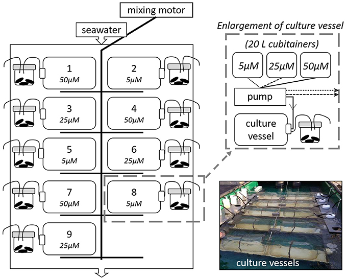
Figure 1. A schematic of the Ecostat experimental setup. The graphic on the left illustrates the flow-through seawater table where the culture vessels were kept. Each culture vessel was randomly assigned to a mixing cradle, which was gently rocked via an electric motor throughout the experiment. Twenty liter cubitainers of treatment water fed each vessel and vessel effluent water subsequently fed a mussel chamber containing three blue mussels (Mytilis edulis). The schematic in the top right shows the links between cubitainers of stock solution, pump, culture vessel, and mussels. The picture in the lower right shows the Ecostat at the onset of an experiment. The continuous culture system (Ecostat) is modified from Grear et al. (2017) and based on Pickell et al. (2009).

FIGURE 2

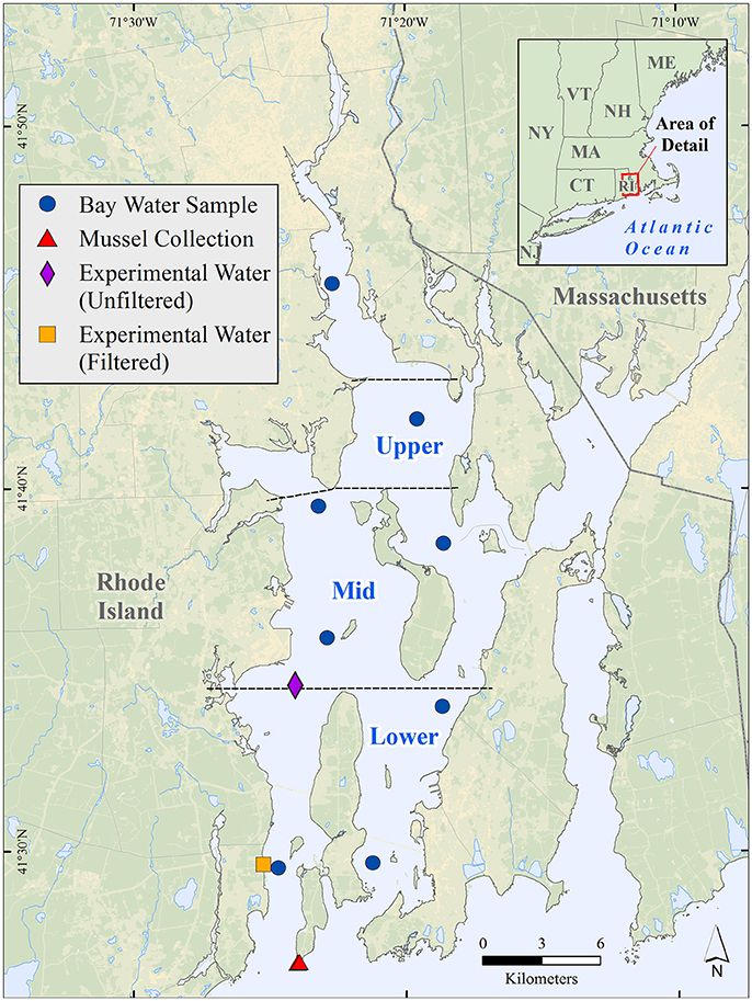
Figure 2. Map of Narragansett Bay (RI, USA) showing station locations for water samples collected from the top, middle, and bottom of the water column at each of eight locations as well as the locations where the mussels and water were collected for use in the Ecostat experiments. Water quality data from December 2014 and December 2015 from the eight stations were grouped by spatial category and incorporated into an empirical model (results presented in Figures 6, 7). The boundaries of our regional groupings are delineated with the dashed lines. The Providence River Estuary is north of the Upper Bay (“Upper”).

Mussels

Juvenile blue mussels (Mytilus edulis) were collected at the mouth of Narragansett Bay, RI USA (Figure 2). Three mussels (TL = 10–15 mm) were measured for length, marked with waterproof paint and placed into acid washed mussel chambers (8 oz./250 ml screw cap polypropylene jars, Nalgene™) with 70 mm screw caps (Figure 1). Mussel chambers were suspended in the mesocosm, just below the water's surface, and received outflow water from a designated polycarbonate culture vessel, through a separate acid washed silicone line (0.64 mm ID, platinum cured). An additional outflow line coming from the top of each mussel chamber insured flow through conditions and allowed flow rates to be measured daily.

Ecostat Sample Collection

Seawater samples were collected five times over the course of each 14-day experiment. This was done by disconnecting the mussel chambers and attaching sample containers to the outflow stream from each of the polycarbonate culture vessels. For chlorophyll analysis, 50 ml seawater samples were filtered through 25 mm GF/F Glass Microfiber Filters (Whatman Plc). The filters were placed in 90:10 acetone/water mixture and stored in a freezer for 24 h before analysis. To obtain particulate samples for stable isotope analysis, the seawater collected from the system was filtered through muffled 25 mm GF/F Glass Microfiber Filters. To ensure that we reached instrument detection, the volume of water filtered varied across each experiment. At the start of each experiment, one liter was filtered. After that, water volumes ranged from 300 ml to 1 l, depending on how quickly the filters clogged. For the October 2015 and March 2016 experiments, 20 ml samples of the filtrate were collected for nutrient analysis and frozen until analyzed at the Nutrient Analytical Services Laboratory at the Chesapeake Biological Laboratory at the University of Maryland Center for Environmental Science.

One mussel from each treatment was collected at the beginning of the experiment and on days 7 and 14. After the day 7 collection another individual was added to the mussel chamber to maintain approximately consistent biomass. Only one mussel for each sampling period/tank was collected due to flow constraints (2 ml) and filtration rates of blue mussels. Filtration rates can vary for small (15 mm) blue mussels based on temperature, salinity, food quality and quantity (Riisgård et al., 2013). However, we believe that the mussels would have been food limited if additional mussels had been added to the chambers. The collected mussel samples were placed in glass vials and frozen. At the beginning and end of the early experiments and during all sampling events in the final experiment, samples were also collected for determination of total alkalinity and dissolved inorganic carbon. Specialized sample containers with vented caps and a tube inlets were used to allow filling from the bottom, thereby minimizing potential atmospheric gas exchange. These samples were immediately preserved with mercuric chloride and stored until analysis.

Isotopes

Particulate samples on the filters were placed into aluminum pans and dried at 60°C for 24 h. The filters were then wrapped in aluminum foil and pelletized for isotopic analysis. Mussels were measured for total length and then their tissues were removed and dried at 60°C for 24 h. Dried tissues were then ground to a fine powder using a mortar and pestle and stored in glass vials until analyzed.

Whole filter and mussel samples (about 1.5 mg) were analyzed using a GV Instruments IsoPrime (Elementar Americas, INC.) continuous flow—isotope ratio mass spectrometer (CF-IRMS). Carbon isotope ratios were determined using a working gas standard (CO₂: 99.99%) and normalized using a three-point calibration line that included the international standards IAEA-CH-3 (cellulose δ¹³C = −24.72‰) and IAEA-C-6 (sucrose: δ¹³C = −10.43‰) and an in-house standard DORM-3 (dogfish tissue: δ¹³C = −19.78‰). Each of these standards was analyzed at the beginning, middle and end of each sample run and reported relative to Vienna Pee Dee Belemenite (δ¹³C) scale. The average relative standard deviation for these triplicate standard runs was 0.7%. A blank sample was also analyzed at the start of each sample run to verify that CO₂ backgrounds were low. As blank levels were always less than 1% of sample values, the data were not blank corrected.

Field Sample Collection and Analyses

As part of a separate ongoing research effort, samples for particulate matter δ¹³C and nutrient analysis were collected monthly at eight stations throughout Narragansett Bay (Figure 2) from December 2014 through December 2015. At each station a Hydrolab Surveyor data logger (Hach Environmental, Loveland, CO) was used to measure temperature, salinity, and pH values at the top, middle, and bottom of the water column. Water samples were collected from these same locations in the water column at each station using a 5 L Go-Flo bottle. Aliquots of water were decanted into 40 ml glass vials, for dissolved inorganic carbon (DIC) analysis, 125 ml bottles for alkalinity titrations, and 1 L bottles for the determination of total suspended solids (TSS) and percent organic matter (%OM). In the former two cases, containers were filled from the bottom and allowed to overfill for approximately 5 s before the final sample was collected. Additional water was decanted into 1 L acid-washed bottles which were stored in the dark, on ice, until processed in the lab. From these 1 L bottles, two replicates of approximately 400 ml were filtered through pre-combusted glass fiber filters (Whatman, 25 mm). The filters were dried in a 60°C oven for at least 24 h and a portion of the filtrate was decanted into acid-stripped 20 ml scintillation vials. The vials were kept frozen until analysis for dissolved inorganic nutrient concentrations.

Stable Isotope Analyses of Field Samples

The filters collected from the field excursions were analyzed using a Elementar Vario Micro elemental analyzer connected to a continuous flow Isoprime 100 isotope ratio mass spectrometer (Elementar Americas, Mt. Laurel, NJ). Replicate analyses of isotopic standard reference materials USGS 40 (δ¹³C = −26.39‰; δ¹⁵N = −4.52‰) and USGS 41 (δ¹³C = 37.63‰; δ¹⁵N = 47.57‰) were used to normalize isotopic values of working standards (blue mussel homogenate) to the Air (δ¹⁵N) and Vienna Pee Dee Belemnite (δ¹³C) scales (Paul et al., 2007). Working standards were analyzed after every 24 samples to monitor instrument performance and check data normalization. The precision of the laboratory standards was ±0.3‰ for carbon and nitrogen.

TSS and % Organic Matter

To prepare glass fiber filters (Whatman, 25 mm) for use in measuring TSS and %OM, they were soaked in distilled, deionized water (DIW) and dried in an 80°C oven. Filters were then ashed at 450°C for 4 h and stored in a desiccator until use. Filter and aluminum dish pairs were weighed and 400–500 ml of sample water was filtered through the pre-weighed filter. Filters and filter funnel were rinsed with about 20 ml of DIW before and after filtration. Filter and dish pairs were then dried overnight at 104°C. Dried filter-dish pairs were then weighed to determine the mass of the TSS sample. The samples were then ashed at 450°C for 4 h, cooled, and then re-weighed. The %OM was determined as the mass of the material lost from the filter after ashing divided by the mass of TSS.

Dissolved Inorganic Carbon Measurements

Two procedures were used for dissolved inorganic carbon (DIC) analysis. For the preserved Ecostat samples from the March and October 2016 experiments, DIC analyses included multiple determinations of DIC in Certified Reference Materials (CRMs) for quality control (Dickson CRM batch 151, http://cdiac.ornl.gov/oceans/Dickson_CRM/batches.html). The samples and CRMs were run on an Apollo AS-C3 DIC analyzer, which uses auto-dilutions to create calibration curves from the CRMs. This instrument acidifies the samples to convert the DIC to carbon dioxide and then measures the carbon dioxide concentration using infrared detection. As an independent check, we analyzed blind samples from the Dickson laboratory (batches 162 and 164) and determined that, on average, our results on the Apollo were near 0.1% uncertainty.

Field samples for DIC were analyzed within a few days of collection. Analytical runs for the field samples, as well as those from the October 2015 experiment, included multiple determinations of DIC in commercial check standards materials (Ultrascientific, Rhode Island, USA). These analyses were performed on a Shimadzu TOC-V Total Organic Carbon Analyzer (Shimadzu Scientific Instruments, Maryland, USA), which uses the same principal of operation as the Apollo described above. Five-point standard curves were used to calibrate sample values and blanks and the independent check standards were measured every 10–15 samples. Uncertainty was within 4%. The “weather quality” standard developed by the Global Ocean Acidification Observing Network defines measurements of sufficient quality to identify relative, short-term variations for mechanistic studies within ecosystems to be ±10 μmol kg⁻¹ (roughly 0.5% for typical seawater; Newton et al., 2015). That requirement is less appropriate for estuarine observations such as ours, where DIC values varied over a range of more than 600 μmol kg⁻¹ (>30% of the mean).

Alkalinity Measurements

A Metrohm Titrino 877 Plus automated titration unit was used to measure total alkalinity (TA) via closed cell titration with a TRIS-calibrated hydrochloric acid and sodium chloride titrant solution. The TA of the sample was estimated from titration data using the non-linear least squares method described in Dickson et al. (2007) and implemented in the seacarb package (R Core Team, 2014), with Certified Reference Materials (batches 128, 137, 139, and 151; http://cdiac.ornl.gov/oceans/Dickson_CRM/batches.html) measured every 10 samples. Overall, measured standards were within 1% of the certified reference values (approximately 0.2% in the blinded analysis of CRM batches 162 and 164 mentioned above).

Carbonate Chemistry Calculations

Concentrations of dissolved carbon dioxide (CO₂), bicarbonate (${\text{HCO}}_3^{-}$), and carbonate (${\text{CO}}_3^{2-}$) and the partial pressure of carbon dioxide (pCO₂) were calculated from DICc, TA, temperature, salinity and pressure using the seacarb package (v.3) in R (R Core Team, 2014) with the Millero (2010) option selected for k1and k2 constants, the Dickson and Riley (1979) option for kf and the Dickson (1990) option for ks.

Statistical/Model Analyses

To examine the relationship between ${\text{HCO}}_3^{-}$ and δ¹³C in the controlled conditions, we used aggregated data from all Ecostat experiments and used linear mixed effects models fitted via maximum likelihood (lme4 package; R Core Team, 2014). The Ecostat vessel was treated as a random effect in the mixed model to account for the expected correlation of repeated measurements made on each vessel. Although δ¹³C was not a directly controlled variable, we treated it as a fixed effect in these linear models. For this and the analysis of field data (see below), we assessed models using corrected Akaike Information Criterion (AICc, Burnham and Anderson, 2002).

We fitted 26 linear mixed effects models to the field measurements of [${\text{HCO}}_3^{-}$]. The predictors included were: (1) δ¹³C; (2) region within the bay (Providence River, Upper Bay, Mid Bay, and Lower Bay); (3) depth layer (surface, mid-depth, bottom); in situ temperature; and percent organic matter (100 × OM fraction of TSS). Since our goal was to identify a relatively simple model with no more than two predictors, the 26-model set included all possible models containing one predictor, two predictors, or two predictors with their interactions.

Results

Primary and Secondary Production

First Experiment, October 2015

In the October 2015 experiment there was evidence of a substantial plankton bloom in all of the treatments (Figure 3), although the bloom was more pronounced in the 25 and 50 μM treatments. DIN concentrations of water collected on the first day of the experiment were 9.4 ± 1.0 μM for the 5 μM treatment, 31.6 ± 7.7 μM for the 25 μM treatment, and 44.4 ± 10.6 μM for the 50 μM treatment. Values declined down to 1.1 ± 0.1 μM for the 5 μM treatment and down to 14.3 ± 1.3 μM for the 25 μM treatment by day 14. Mean DIN concentrations in the 50 μM were always >40 μM. Prior to the start of the experiment, water column chlorophyll concentrations were about 3.5 μg l⁻¹. By day four the chlorophyll concentrations in the treatments exceeded 35 μg l⁻¹, and remained elevated for the duration of the experiment. In contrast, chlorophyll concentrations in the 5 μM treatment were roughly around 8 ug l⁻¹. The plankton δ¹³C values closely tracked the chlorophyll concentrations (Figure 4), where values in the higher two treatments jumped up about 6‰, from about −23‰ to −17.4 ± 0.3‰ in the 25 μM and to −16.8 ± 0.1‰ in the 50 μM by day 4. By day 7, δ¹³C values in the two enriched tanks were −15.3 ± 0.4‰ and −14.8 ± 0.5‰ for the 25 and 50 μM treatments, respectively. They remained similarly elevated for the duration of the experiment. While δ¹³C values in the 5 μM treatment vessels increased, with a peak at day 4 (−20.1 ± 0.3‰), values only increased about 1.5‰ over the duration of the experiment (from −23.2 to roughly −21.5‰). The mussel δ¹³C values closely tracked the plankton values, where mussel δ¹³C values in the 25 and 50 μM treatments increased about a per mil (to ~ −18.7‰) in the first week of the experiment and then another 1.5‰ (25 μM) and 2.0‰ (50 μM) in the second week (Figure 4). At the end of the experiment, mussel δ¹³C values were −19.1 ± 0.3‰, −16.0 ± 0.1‰, and −15.5 ± 0.2‰ in the 5, 25, and 50 μM treatments. These values were similar to those of the phytoplankton on day 14 (−21.4 ± 0.9‰, −16.5 ± 0.2‰, and −15.1 ± 0.1‰ for the 5, 25, and 50 μM treatments, respectively; Figure 4).

FIGURE 3

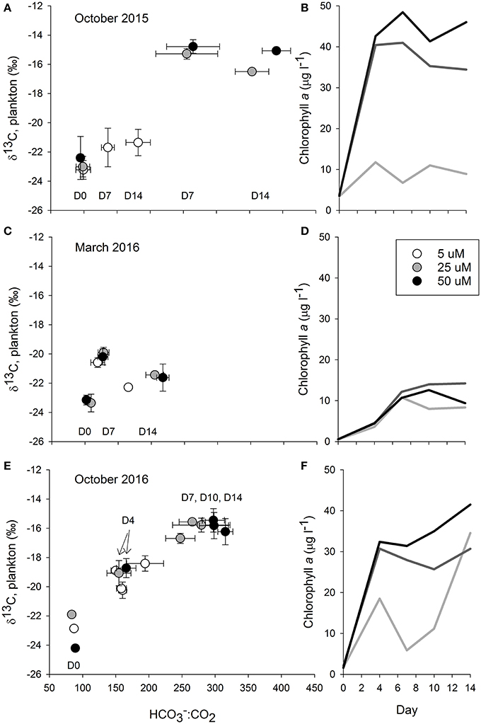
Figure 3. The graphs in the left column plot bicarbonate to dissolved carbon dioxide ratios (${\text{HCO}}_3^{-}$:CO₂) against δ¹³C values measured in plankton from the October 2015 (A,B), March 2016 (C,D), and October 2016 (E,F) Ecostat experiments. The carbonate parameters were calculated from measurements of temperature, salinity, and alkalinity in the effluent water stream while the δ¹³C values were from plankton captured on glass fiber filters. As the resultant relationships were roughly chronological, we indicated the day of the experiment using the notation D for day followed by the experimental day (e.g., D7 is day seven). The color of the circle and or line corresponds to the level of nutrient enrichment, with darker colors indicating higher enrichment. Error bars show the standard deviation around the means of the three replicate treatments for both the X and Y axes. Chlorophyll concentrations from each of the three experiments are given, over time, in the right column. The shading of the lines corresponds to the level of treatment where the lighter color is associated with the lower enrichment (5 μM) and the darkest color with the highest enrichment (50 μM).

FIGURE 4

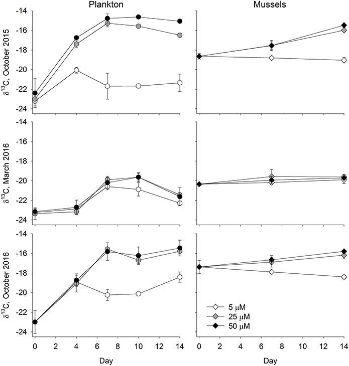
Figure 4. Particulates (A,C,E) and Mussels (B,D,F) δ¹³C values for the October 2015 (A,B), March 2016 (C,D), and October 2016 (E,F) Ecostat experiments. Given that the seawater used in this experiment screened, and a portion was filtered, prior to the experiment, we presume that the particulate values shown in the left column largely represent phytoplankton. Error bars show the standard deviation around a mean of samples from 3 replicate culture vessels.

Second Experiment, March 2016

The biological response to the nutrient enrichments was far less in the March 2016 experiment than it was in the prior October 2015 experiment (Figure 3). The DIN concentrations on the first day of the experiment were similar to those from October 2015, where DIN was 8.9 ± 1.0 μM for the 5 μM treatment, 25.5 ± 0.7 μM for the 25 μM treatment, and 51.7 ± 1.6 μM for the 50 μM treatment. Values declined down to 3.0 ± 0.3 μM and 1.7 ± 0.4 μM for the 5 and 25 μM treatments, respectively, by day 14. Mean DIN concentrations in the 50 μM were 18.2 ± 3.7 μM. The chlorophyll concentrations at the beginning of the experiment were lower, ranging from 0.5 to 0.6 μg l⁻¹ among the treatments, than in the prior and subsequent experiments. By day 4, chlorophyll increased to 3.6 μg l⁻¹ in the 5 μM treatment and ~4.5 μg l⁻¹ in the 25 and 50 μM treatments. While concentrations further increased over the course of the experiment, they ranged from 9.4 to 14.2 μg l⁻¹ in all treatments, and were less than those measured previously. Similarly, weak responses were measured in the plankton and mussel δ¹³C values (Figure 4). Plankton δ¹³C values started at about −23.2‰ and increased to a maximum of −19.7‰ in the two more enriched treatments. Mean mussel δ¹³C values for each treatment ranged from −20.4 to −19.6‰ over the course of the experiment, across all three treatments (Figure 4).

Third Experiment, October 2016

While nutrient data were not available in the third experiment, there was a clear and swift response in the nutrient augmented treatments (Figure 3). Starting chlorophyll concentrations were 1.6–2 μg l⁻¹ and by day 4, concentrations were 19 μg l⁻¹ in the low nutrient treatment and >30 μg l⁻¹ in the other two treatments. While the 25 and 50 μM treatments generally maintained these elevated chlorophyll concentrations throughout the experiment, the 5 μM treatment was far more variable. Again, these patterns were also reflected in the δ¹³C values of the phytoplankton. While δ¹³C values started at −23‰, they quickly jumped 4‰, up to −19‰, by day 4 and, by day 7, values exceeded −16‰ in the two most enriched treatments (Figure 4). As in the October 2015 experiment, the δ¹³C values in the blue mussels from the October 2016 experiment generally tracked the plankton δ¹³C values. Initial mussel δ¹³C values were −17.4 ± 0.7‰ and the low enrichment (5 μM) treatment remained <−17‰ for the duration of the experiment (Figure 4). In contrast, the mussels being fed with effluent from both the 25 and 50 μM treatments had increased δ¹³C values at days 7 and 14, where the mussels receiving water from the 25 μM treatments increased about 0.5‰ between each sampling day (days 0, 7, and 14), while the increase in the 50 μM treatments was about 0.7‰ between each time step (Figure 4).

Carbonate Chemistry

In response to the nutrient additions, and presumably in response to the associated changes in the production in the treatment vessels, the carbonate chemistry changed in each tank, across all of the experiments (Figure 3, Table 1). The [${\text{HCO}}_3^{-}$] and [CO₂] both decreased over the course of each of the experiments, as production increased and DIC was consumed (Table 1). However, the relative proportions of ${\text{HCO}}_3^{-}$:CO₂, increased over time. If proportionally more ${\text{HCO}}_3^{-}$ led to more ${\text{HCO}}_3^{-}$ uptake, then the higher δ¹³C values associated with ${\text{HCO}}_3^{-}$ would be reflected in the plankton and mussels (e.g., Fogel et al., 1992; Oczkowski et al., 2008, 2014). While these ratios shifted for each treatment in each experiment, the effects were more pronounced in the October 2015 and October 2016 experiments, especially in the 25 and 50 μM treatments (Figure 3). The ratio increased with increased production and, when plotted against plankton δ¹³C values, the temporal aspects of the experiment were reflected. Patterns in plots of plankton δ¹³C vs. ${\text{HCO}}_3^{-}$:CO₂ closely mirror trends in chlorophyll over time as the relationships between δ¹³C and ${\text{HCO}}_3^{-}$:CO₂ are positive over the course of the experiments (Figure 3). Further, there was a positive relationship between chlorophyll and plankton δ¹³C values (as implied by Figure 3) and negative relationships between plankton δ¹³C values and [${\text{HCO}}_3^{-}$] and [CO₂] (Figure 5). DIN concentrations also decreased over the course of the first two experiments (when data were available). We aggregated each individual measurement of [${\text{HCO}}_3^{-}$] and δ¹³C values to define a linear relationship such that predicted [${\text{HCO}}_3^{-}$] = 703–46.5 × δ¹³C (Figure 5) to determine whether the Ecostat relationships, in conjunction with measured δ¹³C values in open water particulate matter (PM), could be used to predict Narragansett Bay water column productivity (Figure 6).

TABLE 1

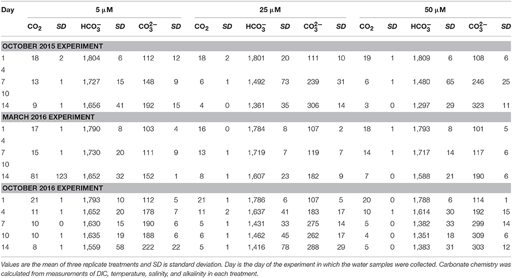
Table 1. Dissolved carbon dioxide (CO₂), bicarbonate (${\text{HCO}}_3^{-}$), and carbonate (${\text{CO}}_3^{2-}$) concentrations, in μmol kg⁻¹, for each of the three Ecostat experiments.

FIGURE 5

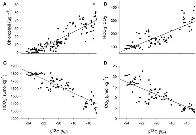
Figure 5. Measured δ¹³C values over the course of all three experiments from all culture vessels plotted against chlorophyll (A), the ratio of bicarbonate to carbon dioxide (B), carbon dioxide (D), and bicarbonate (C) concentrations that were collected at the same time. Regressions were all highly significant (p < 0.001) where the regression equation for δ¹³C against chlorophyll was y = 4.80x+113 (R² = 0.81), against ${\text{HCO}}_3^{-}$:CO₂ was y = 23.4x+644 (R² = 0.71), against CO₂ was y = −1.48x−18.2 (R² = 0.71), and against ${\text{HCO}}_3^{-}$ was y = −46.5x+703 (R² = 0.79).

FIGURE 6

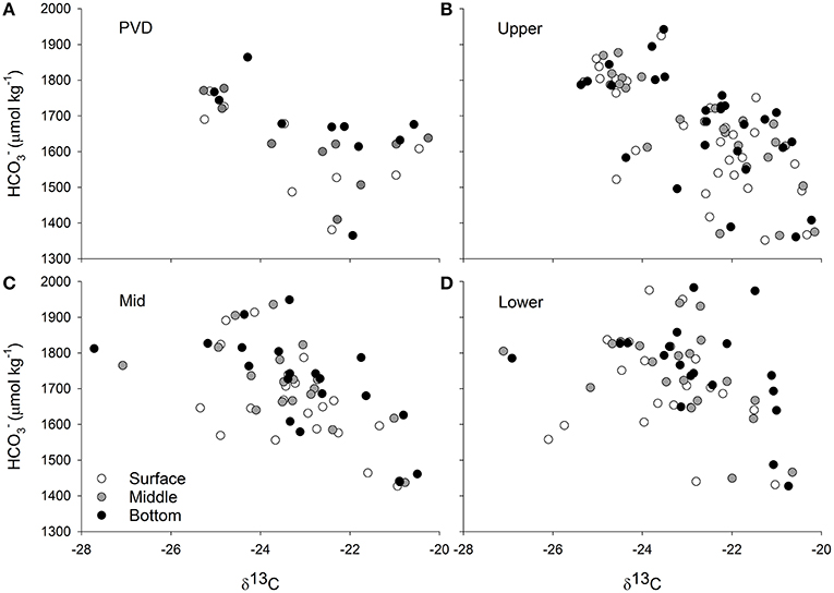
Figure 6. Carbon stable isotope values measured on particulate matter collected from eight stations in Narragansett Bay (Figure 2) and at three depths (surface, middle of the water column, and bottom) are plotted against bicarbonate concentrations at the same station and water column position. Stations are grouped by region where PVD is the Providence River Estuary (A), Upper is the Upper Bay (B), Mid is the Middle of Narragansett Bay (C), and Lower is the Lower Bay (D). The ${\text{HCO}}_3^{-}$ concentrations were calculated from dissolved inorganic carbon and total alkalinity measurements of water samples and from temperature and salinity measurements made in the field. Methodological details are given in the text.

Narragansett Bay Water Column

While coarser than the relationships observed in the Ecostat experiments, there were significant relationships between calculated water column [${\text{HCO}}_3^{-}$] and δ¹³C values in the Upper and Mid portions of Narragansett Bay (Figure 6) but depth (water column position), temperature, and region did not significantly affect the relationship between [${\text{HCO}}_3^{-}$] and δ¹³C values.

The relationships between δ¹³C values and [${\text{HCO}}_3^{-}$] established in the Ecostat experiments, using measurements from all three experiments, were used to predict carbonate chemistry in Narragansett Bay. We used approximately monthly particulate matter δ¹³C values from samples collected at the surface, mid, and bottom of the water column at each of eight stations in Narragansett Bay. The Bay PM δ¹³C values were used to predict [${\text{HCO}}_3^{-}$] using the relationship of Y = 703 − 46.5 × δ¹³C that was established via the Ecostat measurements (R² = 0.79, Figure 5). These predictions were then visually compared in Figure 7 to the in situ “bottle” [${\text{HCO}}_3^{-}$] calculated from DIC and TA bottle samples; the modeled relationship of in situ [${\text{HCO}}_3^{-}$] with in situ δ¹³C, and the modeled relationship of in situ [${\text{HCO}}_3^{-}$] with in situ δ¹³C and %OM and their interaction. This latter model was included because it emerged as the best model within our search for a model of [${\text{HCO}}_3^{-}$] containing no more than two predictor variables from the field data set (see Table 2 and its caption for further explanation). Based on log likelihood (and deviance, which can be calculated as −2 * log likelihood), this model had the highest goodness-of-fit among all the candidate models. Based on evidence ratios (see section 2.10 in Burnham and Anderson, 2002), this model is more likely than any model in the set, by a factor >99:1, to be the selected best model if the same Narragansett Bay processes were resampled in an independent study.

FIGURE 7

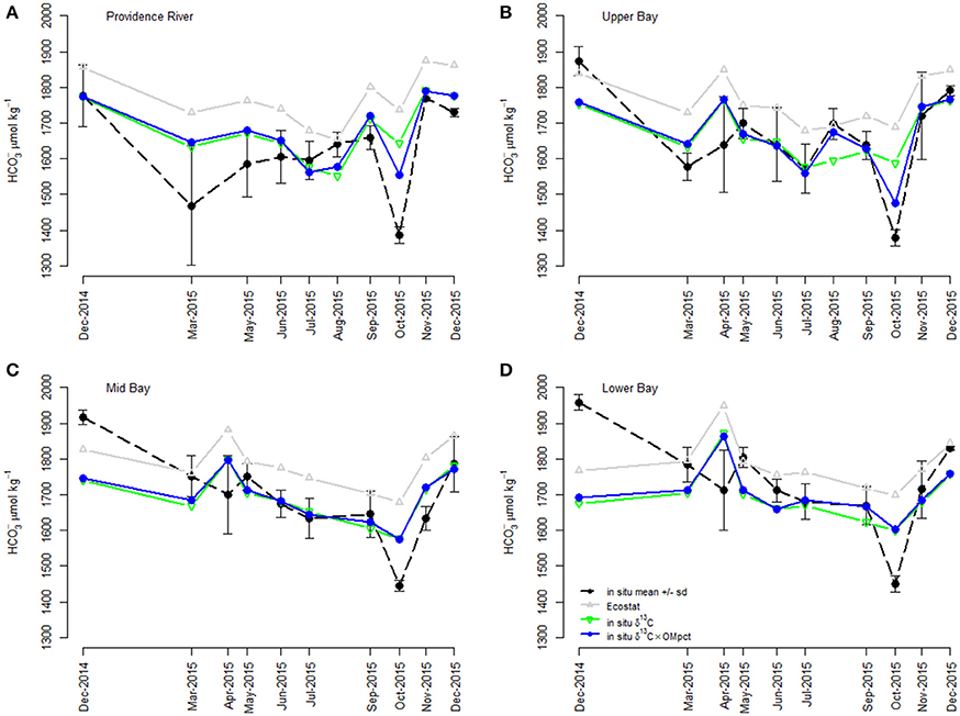
Figure 7. Comparison of Ecostat-based predictions and empirical field-based models of [${\text{HCO}}_3^{-}$] in Narragansett Bay. The “in situ” points refer to [${\text{HCO}}_3^{-}$] calculated from DIC and TA in bottle samples from Narragansett Bay. “Ecostat” refers [${\text{HCO}}_3^{-}$] prediction via substitution of in situ δ¹³C into the regression of [${\text{HCO}}_3^{-}$] against δ¹³C in the Ecostat experiments. “In situ δ¹³C” and “in situ δ¹³C and OM” refer to predictors in their respective empirical relationship with in situ [${\text{HCO}}_3^{-}$]. The model containing δ¹³C and OM was the best empirical model of the field observations. Although the relationships are shown separately for each region within the bay for visual clarity, including region in the empirical models improved neither the goodness of fit (i.e., log-likelihood) nor the parsimony (i.e., AICc; see Table 2). The regions of the Bay [e.g., Providence River (A), Upper Bay (B), Mid Bay (C), and Lower Bay (D)] are shown in Figure 2.

TABLE 2

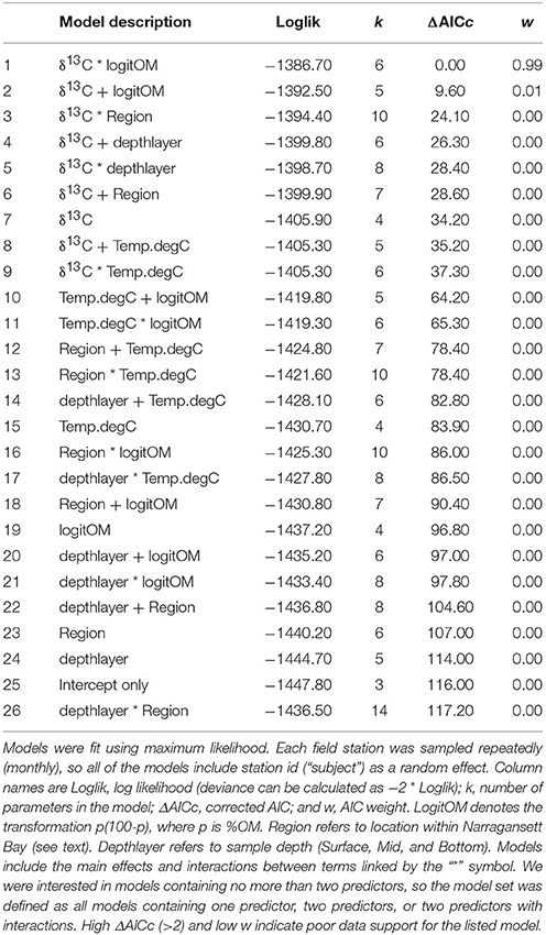
Table 2. AIC-based model selection results for linear mixed effects models of [${\text{HCO}}_3^{-}$] in in situ bottle measurements, ordered from best to worst.

The simple estimates of [${\text{HCO}}_3^{-}$] obtained from application of the Ecostat regression appeared to trend similarly (i.e., in parallel) to the observed concentrations and to “in situ δ¹³C model,” particularly in the Providence River Estuary and Upper Bay (Figure 7). Finally, the best approach for predicting in situ [${\text{HCO}}_3^{-}$] among our set was the “in situ δ¹³C and OM model” without the Ecostat-derived parameters. Since the field samples for DIC were not preserved prior to analysis, loss of DIC from the samples probably contributed to the offset between Ecostat- and field-based predictions. However, we interpret the close parallel trend of the Ecostat-based results as evidence that the same mechanisms were at play in the experiments and field observations. In general, the δ¹³C-based estimates of [${\text{HCO}}_3^{-}$] tended to over-predict concentrations and the data fell within a narrower range overall. The addition of the OM predictor reduced this over-prediction.

Discussion

While all three Ecostat experiments yielded consistent results, only two of the three responded to the nutrient enrichment via phytoplankton blooms. The 2015 and 2016 October experiments demonstrated clear and distinct responses. These responses were documented in the chlorophyll concentrations, carbonate chemistry, and stable isotopes of both the plankton and the mussels. While both [${\text{HCO}}_3^{-}$] and [CO₂] declined over the course of the experiments, the ratio of ${\text{HCO}}_3^{-}$:CO₂ increased. The shift in the ratio is likely due to different rates of drawdown of CO₂ and ${\text{HCO}}_3^{-}$ (e.g., Oczkowski et al., 2014). In contrast, while the results were consistent with the October measurements, the response to the nutrient enrichment was more subdued in the March 2016 experiment. The primary reason for the difference between this and the other experiments likely was the smaller phytoplankton community at the onset of the experiment. While the time 0 chlorophyll concentrations were approximately 3.5 and 1.8 μg l⁻¹ for the October 2015 and 2016 experiments, respectively, they averaged about 0.5 μg l⁻¹ in the March experiment. Overall, however, it was clear across all three experiments that the carbon stable isotope values in the phytoplankton, and in the mussels that consumed them, were closely linked to the chlorophyll concentrations as well as to the carbonate chemistry.

Increases in plankton carbon isotope values were substantial in all three experiments and δ¹³C values were very similar, often indistinguishable, between the 25 and 50 μM treatments. For example, in these treatments during the first experiment (October 2015), the δ¹³C values of the plankton increased by more than 5.5‰ in just 4 days (Figure 4). Differences between final and initial δ¹³C values were roughly 8‰ at the end of the two-week experiment in both the 25 and 50 μM treatments. Even a small enhancement of 5 μM DIN (and 1.2 μM PO₄) led to an almost 2‰ increase in phytoplankton δ¹³C values. Similar observations were made in the third experiment (October 2016). These changes in the δ¹³C values characterizing the plankton were subsequently reflected in the blue mussels being fed by the Ecostat effluent water, and their tissues reflected the enrichment as early as seven days into the experiment (Figure 4). The final enrichment was about 2.8‰ (2.6 and 3.0‰ in the 25 and 50 μM treatments, respectively) in the October 2015 experiment and about 1.4‰ (1.2 and 1.6‰ in the 25 and 50 μM treatments) in the October 2016 experiment. Given the length of these experiments (14 days), these shifts are remarkable, as is the sensitivity of the organisms to relatively small changes in carbonate chemistry (Table 1). Drawdown of DIN concentrations over the course of the October 2014 and March 2015 experiments (where data were available) further support the observations of rapid ecological response. While the initial δ¹³C values varied, the blue mussel tissues closely aligned with the plankton δ¹³C values at the conclusion of each of the three experiments. The δ¹³C values of the mussels increased to match that of their food source and thus the offsets between initial and final values were dictated by the final food source δ¹³C values.

Our Ecostat experiments support the conclusion made by Oczkowski et al. (2014) that carbon isotopes can sensitively track plankton blooms in estuarine waters. The subtler responses of the March 2016 experiment also indicate that δ¹³C values may not as effectively track smaller scale shifts in plankton abundance, especially given that estuarine water columns are a mix of plankton and detritus.

Field Applications

The laboratory experiments used a “clean water column” to focus on the phytoplankton response to the nutrient enrichments. By using a mix of approximately 1/3 raw (but screened at 150 μm) and 2/3 filtered seawater, most of the detritus and grazers were removed. While the Ecostat experiments demonstrated the links between nutrients, production, carbonate chemistry, and δ¹³C values in estuarine waters, these linkages were less clear in situ. As the relative proportion of new production to detrital material varies with season, position in the water column, and position in the estuary, only peaks in production (and associated high δ¹³C values) may be discernable from the noise of a mixed system (e.g., Oczkowski et al., 2014) as δ¹³C reflects all the organic matter on the filter, not just the plankton. Further, it is important to be clear that the δ¹³C-predicted [${\text{HCO}}_3^{-}$] and bottle calculated [${\text{HCO}}_3^{-}$] are reflecting two different things. The former, which is based on a mix of plankton and detrital organic matter, is representing the carbonate dynamics at the location where the plankton were formed. The latter reflects the carbonate dynamics in the location where the plankton were collected. As field stations are not closed systems, these two measurements may not be reflecting the same water column.

The application of relationships established in the Ecostat experiments to stable isotope values from Narragansett Bay demonstrate the usefulness of δ¹³C for understanding nutrient impacts on carbonate chemistry. Overall, there were coarse temporal relationships between PM-δ¹³C and [${\text{HCO}}_3^{-}$] in Narragansett Bay, particularly in the Providence River Estuary and Upper Narragansett Bay (Figure 6) even with the large uncertainty (about 4%) in the measurements of carbonate chemistry. Accounting for organic matter present in the water column further improved the linear mixed-effects models in the Providence River Estuary and Upper Bay. The %OM had less of an influence on the Mid and Lower regions of Narragansett Bay. The bulk of the bay-wide production occurs in the northern parts of the system, where most of the sewage effluent is received. Thus, the stronger influence of organic matter on carbonate chemistry in the Providence River and Upper Bay is logical (Narragansett Bay Estuary Program, 2017). Sewage effluent is still an important source of nutrients to the whole Bay, with nitrogen stable isotope values characteristic of sewage effluent reflected in primary producers and consumers throughout the system (Oczkowski et al., 2017). But, in the overall less productive Mid and Lower Bay, the amount of organic matter (detritus and plankton) in these regions had less of an influence on the model.

When the relationships established in the Ecostat dataset were applied to the field data, they consistently resulted in over-prediction of [${\text{HCO}}_3^{-}$], although they did trend similarly (Figure 7). The offset between the Ecostat estimated and modeled [${\text{HCO}}_3^{-}$] is attributable to a high intercept on the Ecostat regression equation. We can only speculate why the intercept was too high, leading to the over prediction of [${\text{HCO}}_3^{-}$] in situ. There may have been more loss of DIC from the field samples than the Ecostat samples due to differences in handling. Or, the offset could be reflecting the fundamental differences between measurements of δ¹³C made in phytoplankton alone, as part of a controlled experiment, vs. the δ¹³C values of particulate matter integrating whole water column processes. The field measurements reflect the mix of plankton and detritus and the δ¹³C values of the plankton themselves reflect the net impact of the whole water column, including benthic exchanges, carbonate dissolution, and the respiration of the full ecosystem. For example, water column respiration would decrease [${\text{HCO}}_3^{-}$] (as pH decreases) and lower δ¹³C, potentially shifting the regression line and subsequent intercept lower as well (Figure 7). More respiration would change the relative proportions of [${\text{HCO}}_3^{-}$] and [CO₂], but increase the overall [DIC] of the system. The controlled nature of the Ecostat experiments was useful for identifying and quantifying linkages between δ¹³C and [${\text{HCO}}_3^{-}$], however, these relationships are part of a more complex puzzle. They exist in situ but reflect the net effects of nutrient enhanced eutrophication as well as water column respiration and other factors like benthic exchange. The strength of these relationships is influenced by the amount of organic matter produced (e.g., Figure 7).

The Usefulness of δ¹³C Values as Indicators of Estuarine Production

Relationships between δ¹³C values in PM and carbonate chemistry have been established for open ocean and upwelling regions (e.g., Laws et al., 1995; Pancost et al., 1997); however, these relationships need to be more quantitatively linked to anthropogenic nutrient inputs and production in estuarine waters. Through a series of Ecostat experiments we quantified these relationships and documented elevated δ¹³C values in both the plankton community and consumers (blue mussels, M. edulis). Although the resultant empirical models over predicted [${\text{HCO}}_3^{-}$] in the Narragansett Bay water column, a linear mixed effects model that accounted for water column organic matter and the δ¹³C values of that organic matter was able to predict [${\text{HCO}}_3^{-}$] with some accuracy. This exercise demonstrated the linkages between nutrients, eutrophication, carbonate chemistry, and stable isotopes of carbon. The observations from the Ecostat experiments are a useful tool to assess contributions from high productivity areas to consumers.

Author Contributions

AO, BT, RP, and JG developed the research plan while AP, RJ, BT and RP led the sample analyses. JG conducted the statistical analyses. AO, BT, RP, AP, and JG wrote the manuscript.

Conflict of Interest Statement

The authors declare that the research was conducted in the absence of any commercial or financial relationships that could be construed as a potential conflict of interest.

Acknowledgments

Thank you to Don Cobb and Rick McKinney for collecting the Narragansett Bay water samples and to Alana Hanson for organizing the sample collection. Adam Kopacsi helped construct the Ecostat while the design and parts of the Ecostat were borrowed from Ed Baker and Suzanne Menden-Deuer's research group at the University of Rhode Island's Graduate School of Oceanography (GSO). We also thank Amanda Montalbano for providing technical support and assistance during the exposure set-up for these studies and Stephanie Anderson, GSO's phytoplankton assistant, for providing valuable chlorophyll data for Narragansett Bay. This is ORD tracking number ORD-023863. The views expressed in this article are those of the authors and do not necessarily represent the views or polices of the U.S. Environmental Protection Agency. Any mention of trade names, products, or services does not imply an endorsement by the U.S. Government or the U.S. Environmental Protection Agency. The EPA does not endorse any commercial products, services, or enterprises.

References

Altieri, A. H., and Gedan, K. B. (2015). Climate change and dead zones. Global Change Biol. 21, 1395–1406. doi: 10.1111/gcb.12754

PubMed Abstract | CrossRef Full Text | Google Scholar

Breitburg, D. L., Craig, J. K., Fulford, R. S., Rose, K. A., Boynton, W. R., Brady, D. C., et al. (2009). Nutrient enrichment and fisheries exploitation: interactive effects on estuarine living resources and their management. Hydrobiologia 629, 31–47. doi: 10.1007/s10750-009-9762-4

CrossRef Full Text | Google Scholar

Burnham, K. P., and Anderson, D. R. (2002). Model Selection and Multimodel Inference. New York, NY: Springer.

Google Scholar

Buskey, E. J. (2008). How does eutrophication affect the role of grazers in harmful algal bloom dynamics? Harmful Algae 8, 152–157. doi: 10.1016/j.hal.2008.08.009

CrossRef Full Text | Google Scholar

Cai, W.-J., Hu, X., Huang, W.-J., Murrell, M. C., Lehrter, J. C., Lohrenz, S. E., et al. (2011). Acidification of subsurface coastal waters enhanced by eutrophication. Nat. Geosci. 4, 766–770. doi: 10.1038/ngeo1297

CrossRef Full Text | Google Scholar

Carmichael, R. H., Hattenrath, T. K., Valiela, I., and Michener, R. H. (2008). Nitrogen stable isotopes in the shell of Mercenaria mercenaria trace wastewater inputs from watersheds to estuarine ecosystems. Aquat. Biol. 4, 99–111. doi: 10.3354/ab00106

CrossRef Full Text | Google Scholar

Cifuentes, L. A., Sharp, J. H., and Fogel, M. L. (1988). Stable carbon and nitrogen isotope biogeochemistry in the Delaware estuary. Limnol. Oceanogr. 33, 1102–1115. doi: 10.4319/lo.1988.33.5.1102

CrossRef Full Text | Google Scholar

Cloern, J. E. (2001). Our evolving conceptual model of the coastal eutrophication problem. Mar. Ecol. Prog. Ser. 210, 223–253. doi: 10.3354/meps210223

CrossRef Full Text | Google Scholar

Cloern, J. E., Abreu, P. C., Cartensen, J., Chauvaud, L., Elmgren, R., Grall, J., et al. (2016). Human activities and climate variability drive fast-paced change across the world's estuarine-coastal ecosystems. Glob. Chang. Biol. 22, 513–529. doi: 10.1111/gcb.13059

PubMed Abstract | CrossRef Full Text | Google Scholar

Dickson, A. G. (1990). Standard potential of the reaction: AgCI(s) + 1/2H2(g) = Ag(s) + HCI(aq), and the standard acidity constant of the ion HSO4 in synthetic sea water from 273.15 to 318.15 K. J. Chem. Thermodyn. 22, 113–127. doi: 10.1016/0021-9614(90)90074-Z

CrossRef Full Text | Google Scholar

Dickson, A. G., and Riley, J. P. (1979). The estimation of acid dissociation constants in seawater media from potentiometric titrations with strong base. I. The ionic product of water. Mar. Chem. 7, 89–99. doi: 10.1016/0304-4203(79)90001-X

CrossRef Full Text | Google Scholar

Dickson, A. G., Sabine, C. L., and Christian, J. R. (2007). Guide to Best Practices for Ocean CO₂ Measurements, Vol. 3. Sidney, BC: PICES Special Publication.

Google Scholar

Feely, R. A., Alin, S. R., Newton, J., Sabine, C. L., Warner, M., Devol, A., et al. (2010). The combined effects of ocean acidification, mixing, and respiration on pH and carbonate saturation in an urbanized estuary. Estuar. Coast. Shelf Sci. 88, 442–449. doi: 10.1016/j.ecss.2010.05.004

CrossRef Full Text | Google Scholar

Flynn, K. J., Clark, D. R., Mitra, A., Fabian, H., Hansen, P. J., Glibert, P. M., et al. (2015). Ocean acidification with (de)eutrophication will alter future phytoplankton growth and succession. Proc. R. Soc. B 282:20142604. doi: 10.1098/rspb.2014.2604

PubMed Abstract | CrossRef Full Text | Google Scholar

Fogel, M. L., Cifuentes, L. A., Velinsky, D. J., and Sharp, J. H. (1992). Relationship of carbon availability in estuarine phytoplankton to isotopic composition. Mar. Ecol. Prog. Ser. 82, 291–300. doi: 10.3354/meps082291

CrossRef Full Text | Google Scholar

Fry, B. (2006). Stable Isotope Ecology. New York, NY: Springer Science+Business Media, LLC.

Google Scholar

Goldman, J. C. (1980). “Physiological processes, nutrient availability, and the concept of relative growth rate in marine phytoplankton ecology,” in Primary Productivity in the Sea, ed P. G. Falkowski (New York, NY: Plenum Press), 179–194.

Google Scholar

Grear, J. S., Rynearson, T. A., Montalbano, A. L., Govenar, B., and Menden-Deuer, S. (2017). pCO2 effects on species composition and growth of an estuarine phytoplankton community. Estuar. Coast. Shelf Sci. 190, 40–49. doi: 10.1016/j.ecss.2017.03.016

CrossRef Full Text | Google Scholar

Hawkins, A. J. (1985). Relationships between the synthesis and breakdown of protein, dietary absorption and turnovers of nitrogen and carbon in the blue mussel, Mytilus edulis L. Oecologia 66, 42–49. doi: 10.1007/BF00378550

PubMed Abstract | CrossRef Full Text | Google Scholar

Jasper, J. P., Hayes, J. M., Mix, A. C., and Prahl, F. G. (1994). Photosynthetic fractionation of 13C and concentrations of dissolved CO2 in the central equatorial Pacific during the last 255,000 years. Paleoceanography 9, 781–798. doi: 10.1029/94PA02116

PubMed Abstract | CrossRef Full Text | Google Scholar

Laws, E. A., Popp, B. N., Bidigare, R. R., Kennicutt, M. C., and Maco, S. A. (1995). Dependence of phytoplankton carbon isotopic composition on growth rate and [CO2)aq: theoretical considerations and experimental results. Geochim. Cosmochim. Acta 59, 1131–1138. doi: 10.1016/0016-7037(95)00030-4

CrossRef Full Text | Google Scholar

Millero, F. J. (2010). Carbonate constant for estuarine waters. Mar. Freshw. Res. 61, 139–142. doi: 10.1071/MF09254

CrossRef Full Text | Google Scholar

Mucci, A., Starr, M., Gilbert, D., and Sundby, B. (2011). Acidification of lower St. Lawrence estuary bottom waters. Atmos. Ocean 49, 206–218. doi: 10.1080/07055900.2011.599265

CrossRef Full Text | Google Scholar

Narragansett Bay Estuary Program (NBEP) (2017). State of Narragansett Bay and Its Watershed. Technical report (Providence, RI). Available online at: http://nbep.org/the-state-of-our-watershed/technicalreport/

Newton, J. A., Feely, R. A., Jewett, E. B., Williamson, P., and Mathis, J. (2015). Global Ocean Acidification Observing Network: Requirements and Governance Plan, 2nd Edn. Avaiable online at: https://www.iaea.org/ocean-acidification/act7/GOA-ON%202nd%20edition%20final.pdf

Nixon, S. W., and Buckley, B. A. (2002). “A strikingly rich zone”—nutrient enrichment and secondary production in coastal marine ecosystems. Estuaries 25, 782–796. doi: 10.1007/BF02804905

CrossRef Full Text | Google Scholar

Nixon, S. W., Oczkowski, A. J., Pilson, M. E. Q., Fields, L., Oviatt, C. A., and Hunt, C. W. (2015). On the response of pH to inorganic nutrient enrichment in well-mixed coastal marine waters. Estuar. Coasts 38, 232–241. doi: 10.1007/s12237-014-9805-6

CrossRef Full Text | Google Scholar

Oczkowski, A., Hunt, C. W., Miller, K., Oviatt, C., Nixon, S., and Smith, L. (2016). Comparing measures of estuarine ecosystem production in a temperate New England estuary. Estuar. Coasts 39, 1827–1844. doi: 10.1007/s12237-016-0113-1

CrossRef Full Text | Google Scholar

Oczkowski, A., Markham, E., Hanson, A., and Wigand, C. (2014). Carbon stable isotopes as indicators of coastal eutrophication. Ecol. Appl. 24, 457–466. doi: 10.1890/13-0365.1

PubMed Abstract | CrossRef Full Text | Google Scholar

Oczkowski, A., Nixon, S., Henry, K., DiMilla, P., Pilson, M., Granger, S., et al. (2008). Distribution and trophic importance of anthropogenic nitrogen in Narragansett Bay: an assessment using stable isotopes. Estuar. Coasts 31, 53–69. doi: 10.1007/s12237-007-9029-0

CrossRef Full Text | Google Scholar

Oczkowski, A., Schmidt, C., Santos, E., Miller, K., Hanson, A., Cobb, D., et al. (2017). “How the distribution of anthropogenic nitrogen has changed in Narragansett Bay (RI, USA) following major reductions in nutrient loads,” in Coastal & Estuarine Research Federation 24th Biennial Conference (Providence, RI).

Pancost, R. D., Freeman, K. H., Wakeham, S. G., and Robertson, C. Y. (1997). Controls on carbon isotope fractionation by diatoms in the Peru upwelling region. Geochim. Cosmochim. Acta 61, 4983–4991. doi: 10.1016/S0016-7037(97)00351-7

CrossRef Full Text | Google Scholar

Paul, D., Skrzypek, G., and Fórizs, I. (2007). Normalization of measured stable isotopic compositions to isotope reference scales—a review. Rapid Commun. Mass Spectrom. 21, 3006–3014. doi: 10.1002/rcm.3185

PubMed Abstract | CrossRef Full Text | Google Scholar

Pedersen, M. F., and Hansen, P. J. (2003). Effects of high pH on a natural marine planktonic community. Mar. Ecol. Prog. Ser. 260, 19–31. doi: 10.3354/meps260019

CrossRef Full Text | Google Scholar

Pickell, L. D., Wells, M. L., Trick, C. G., and Cochlan, W. P. (2009). A sea-going continuous culture system for investigating phytoplankton community response to macro- and micro-nutrient manipulations. Limnol. Oceanogr. Methods 7, 21–32. doi: 10.4319/lom.2009.7.21

CrossRef Full Text | Google Scholar

Rau, G. H. (1994). “Variations in sedimentary organic δ13C as a proxy for past changes in ocean and atmospheric CO2 concentrations,” in Carbon Cycling in the Glacial Ocean: Constraints on the Ocean's Role in Global Change, eds R. Zahn, Th. F. Pedersen, M. A. Kaminski, and L. Labeyrie (Berlin; Heidelberg: Springer), 307–321.

Google Scholar

R Core Team (2014). R: A Language and Environment for Statistical Computing, Version 3.1.2. Vienna: R Foundation for Statistical Computing.

Riisgård, H. U., Lüskow, F., Pleissner, D., Lundgreen, K., and López, M. Á. P. (2013). Effect of salinity on filtration rates of mussels Mytilus edulis with special emphasis on dwarfed mussels from the low-saline Central Baltic Sea. Helgoland Mar. Res. 67, 591–598. doi: 10.1007/s10152-013-0347-2

CrossRef Full Text | Google Scholar

Vitousek, P. M., Aber, J. D., Howarth, R. W., Likens, G. E., Matson, P. A., Schindler, D. W., et al. (1997). Human alteration of the global nitrogen cycle: sources and consequences. Ecol. Appl. 7, 737–750. doi: 10.1890/1051-0761(1997)007[0737:HAOTGN]2.0.CO;2

CrossRef Full Text | Google Scholar

Wainright, S. C., and Fry, B. (1994). Seasonal variation of the stable isotopic compositions of coastal marine plankton from Woods Hole, Massachusetts and Georges Bank. Estuaries 17, 552–560. doi: 10.2307/1352403

CrossRef Full Text | Google Scholar

Wallace, R. B., Baumann, H., Grear, J. S., Aller, R. C., and Gobler, C. J. (2014). Coastal ocean acidification: the other eutrophication problem. Estuar. Coast. Shelf Sci. 148, 1–13. doi: 10.1016/j.ecss.2014.05.027

CrossRef Full Text | Google Scholar

Weisse, T., and Stadler, P. (2006). Effect of pH on growth, cell volume, and production on freshwater ciliates, and implications for their distribution. Limnol. Oceanogr. 51, 1708–1715. doi: 10.4319/lo.2006.51.4.1708

CrossRef Full Text | Google Scholar

Zhang, J., Quay, P. D., and Wilbur, D. O. (1995). Carbon isotope fractionation during gas-water exchange and dissolution of CO2. Geochim. Cosmochim. Acta 59, 107–114. doi: 10.1016/0016-7037(95)91550-D

CrossRef Full Text | Google Scholar