Predicting Heat Stress to Inform Reef Management: NOAA Coral Reef Watch's 4-Month Coral Bleaching Outlook

Introduction

Mass coral bleaching due to anomalously warm water temperatures has occurred with increasing frequency and severity in recent decades (Eakin et al., 2010; Heron et al., 2016a; Hughes et al., 2018). It is now the most significant single contributor to the decline of coral reef ecosystems on a global scale (Wilkinson, 2008; Spalding and Brown, 2015). Coral bleaching occurs when the symbiotic relationship between corals and the microscopic algae (zooxanthellae) living in their tissues breaks down due to environmental stress (Jaap, 1979; Jokiel and Coles, 1990). After most zooxanthellae are expelled, the underlying white calcium carbonate coral skeleton becomes visible through the transparent coral tissue; this phenomenon is known as bleaching. Heat stress that persists for several weeks, with ambient water temperatures as little as 1–2°C above a coral's tolerance level, has been shown to cause bleaching (Glynn and D'Croz, 1990; Berkelmans and Willis, 1999). While bleached corals can die due to lack of food produced by symbiotic zooxanthellae if the stress is severe or long lasting, more frequently, death results when weakened corals are infected with subsequent disease (Miller et al., 2009; Rogers et al., 2009; Eakin et al., 2010). Extensive bleaching events have dramatic, long-term, ecological, economic, and social impacts (Baker et al., 2008; Munday et al., 2008; Doshi et al., 2012). Even under favorable conditions, it can take decades or longer for severely bleached reefs to recover, and if they do, it is usually with reduced species diversity and a loss of important reef-building species (Wilkinson, 2008).

The U.S. National Oceanic and Atmospheric Administration's (NOAA) Coral Reef Watch (CRW) program has provided critical information to coral reef managers and scientists based on near real-time satellite monitoring of the heat stress that can cause mass coral bleaching since 1997 (Liu et al., 2006, 2013). As many actions laid out in bleaching preparedness or response plans are expensive and require significant planning (Maynard et al., 2009), marine resource managers have long requested information on the likelihood of bleaching months in advance to prepare for upcoming events (e.g., Tommasi et al., 2017). In 2008, CRW partnered with NOAA's Earth System Research Laboratory to release the world's first global prediction tool for mass coral bleaching heat stress weeks-to-months in advance (Liu et al., 2009). It was based on weekly predictions from a statistical global sea surface temperature (SST) forecast system using the Linear Inverse Modeling (LIM) approach (Penland and Matrosova, 1998) and observed data (1° weekly Optimum Interpolation SST (OISST); Reynolds et al., 2002). This pioneer tool was limited to a single, deterministic forecast of the heat stress that can cause coral bleaching with a coarse spatial resolution of 2°. Subsequently, researchers at the Australian Bureau of Meteorology (BoM) developed a probabilistic bleaching forecast system focused on the Great Barrier Reef based on the Predictive Ocean Atmosphere Model for Australia (POAMA) developed by BoM and the Commonwealth Scientific and Industrial Research Organisation (CSIRO; Spillman et al., 2011, 2013).

Through partnership with the NOAA National Centers for Environmental Prediction (NCEP), in July 2012, CRW released its first probabilistic global subseasonal-to-seasonal-scale Coral Bleaching Outlook system (Eakin et al., 2012). It was based on 9-month SST predictions from NCEP's operational Climate Forecast System Version 1 (CFSv1) (Saha et al., 2006). CFSv1, implemented in August 2004, was NCEP's first quasi-global, fully coupled atmosphere–ocean–land model for seasonal prediction. CFSv1 was a dynamical modeling system that, for the first time in the history of U.S. operational seasonal prediction, demonstrated a level of skill in many predicted fields that was comparable to the skill of the statistical methods used by the NCEP (Saha et al., 2006). Saha et al. (2006) indicated that the CFS had an acceptably low bias in tropical SST prediction and a level of skill in forecasting Niño-3.4 SST better than persistence and comparable to statistical methods used operationally at NCEP and was a large improvement over the previous operational coupled model at NCEP. Barnston et al. (2012) also concluded that the current generation of dynamical seasonal forecast systems, including CFSv2, has a skill better than the statistical seasonal forecast system in predicting Niño-3.4 SST. CRW's probabilistic Bleaching Outlook Version 1 was at a spatial resolution of 1° and updated weekly. This version of the Outlook also used the 1° weekly OISST (Reynolds et al., 2002), which NCEP utilized for initial conditions and skill analysis of the CFS (Saha et al., 2006, 2010, 2014), to calculate accumulated stress at short lead-times.

After the CFS Version 2 (CFSv2) became available in March 2011 (Saha et al., 2014), CRW upgraded its Outlook system. Evaluation of the CFSv2 hindcasts by Saha et al. (2014) showed that CFSv2 significantly improved global SST forecasts over CFSv1 on the seasonal and subseasonal scales, with relatively higher skill in the tropical Pacific than the rest of the globe. CRW's probabilistic Outlook Version 2, released in December 2012, used the CFSv2 9-month SST predictions but maintained the same 1° spatial resolution. The Outlook Version 3, released in February 2015, matched the native spatial resolution of the CFSv2 (0.5°) and used the daily OISST Version 2 (dOISSTv2) at 0.25° resolution (Reynolds et al., 2007; Banzon et al., 2016) for short lead-times. The Outlook Version 4, released in May 2017, subsequently incorporated three daily runs of 90-day predictions and nine daily runs of 45-day predictions, which quadrupled the number of model runs used in the short-term ensembles.

The third, longest, and most widespread global coral bleaching event on record started in the Commonwealth of the Northern Mariana Islands (CNMI) and Guam in June 2014 (Heron et al., 2016b; Eakin et al., 2017). It continuously affected coral reefs around the world until May 2017, when it appeared the global extent of the event had ended (Eakin et al., 2017). Reported impacts to reefs worldwide have been greater than from any previously documented global bleaching event (Eakin et al., 2017; Hughes et al., 2017). CRW's Outlooks, along with its near real-time satellite monitoring, provided critical guidance to coral reef managers, scientists, and other stakeholders throughout the tropics leading up to and during this event (e.g., Eakin et al., 2017; Hughes et al., 2017; Tommasi et al., 2017).

In this article, CRW's probabilistic 4-Month Coral Bleaching Outlook Version 3 system is detailed, as are enhancements in the newest Outlook Version 4. Initial results from the Outlook skill analysis performed on Version 3 are also discussed. Finally, applications of the Outlook by users during the third global bleaching event are demonstrated.

Data

Climate Forecast System Version 2 SST

CRW's probabilistic 4-Month Outlook Versions 3 and 4 use SST predictions from NCEP's CFSv2, a global, fully coupled atmosphere-ocean-sea ice-land, dynamical, seasonal prediction system made operational in March 2011 (Saha et al., 2010, 2014).

CFSv2's ocean component has global coverage. Its meridional resolution is 0.25° between 10°S and 10°N, gradually increasing poleward to 0.5° at 30°S and 30°N; its zonal resolution is 0.5° globally. CRW interpolates the SST predictions to a uniform 0.5° resolution before ingesting them into the Outlook system. The ocean model has 40 vertical layers, with 27 layers in the upper 400 m and a bottom depth of approximately 4.5 km. Its vertical resolution is 10 m from the surface to 240 m depth, gradually increasing to about 500 m in the bottom layer. Predicted temperatures of the top layer (top 10 m) are used as the predicted SST in CRW's Outlook system. The predicted SST represents the daily averaged value through both day and night.

The near real-time operational CFSv2 has 16 runs daily: four producing daily predictions out to 9-months; three out to one season (between about 90 and 120-days); and nine out to 45-days. All predictions are initialized using ocean, atmosphere, and land conditions from the operational Climate Data Assimilation System Version 2 (CDASv2; Saha et al., 2014). The four 9-month runs are control runs and are based on initial conditions at 0000, 0600, 1200, and 1800 UTC. The remaining 12 runs are initialized with perturbed initial conditions (X. Wu, pers. comm.), such that the three 3-month runs begin at 0000 UTC, and the nine 45-day runs begin at 0600, 1200, and 1800 UTC (three runs at each time). CRW's Outlook Version 3 used only the predictions from the four 9-month runs; the Outlook Version 4 uses all 16 runs to increase the number of ensemble members for the near-term Outlook.

The CFSv2 SST hindcasts were used to derive the Outlook's climatologies. The hindcasts contained daily predictions from four 9-month runs initialized at 0000, 0600, 1200, and 1800 UTC on every fifth day, based on the regular calendar year, starting on January 1 each year, from 1982 to 2010 (see Table B1 of Saha et al., 2014). Thus, the hindcasts were run on the same calendar dates every year; February 29 in a leap year was ignored. The initial conditions were from the Climate Forecast System Reanalysis (CFSR) (Saha et al., 2014).

Daily OISST Version 2

For each predicted day, CRW's Outlook requires daily SST values from the 12-weeks leading up to the predicted day (see the Methods section). Hence, predicting heat stress for any day within 12-weeks of the initial condition day needs historical SST values; the daily SST from the dOISSTv2 (Reynolds et al., 2007; Banzon et al., 2016) is used. This widely used dOISSTv2 dataset, an operational near real-time NOAA/National Environmental Satellite, Data, and Information Service (NESDIS) SST analysis, combines satellite and in situ measurements to produce a day-night blended SST analysis. CRW's Outlook utilizes the version of dOISSTv2 that is based on satellite data from only the Advanced Very High Resolution Radiometer (AVHRR) satellite sensors.

Complementing the near real-time dOISSTv2, NESDIS produces a reprocessed version in a 14-day delay mode, providing a long-term data record (1981-present). For its Outlook system, CRW used the reprocessed dOISSTv2 to develop the climatology required for deriving the historical heat stress variables for the initial condition day, and earlier days, of each near real-time CFSv2 run.

Methods

The Outlook was developed to emulate, with minor modifications, the algorithm used in CRW's near real-time operational satellite coral bleaching heat stress monitoring (Liu et al., 2013, 2014). From the CFSv2 SST predictions, the Outlook system generates model-based versions of CRW's daily satellite Coral Bleaching HotSpot, Degree Heating Week (DHW), and Bleaching Alert Area variables.

The first two of the following four subsections (i.e., Climatology and Bleaching Heat Stress Metrics) describe how the Outlook algorithm was developed based on CRW's satellite algorithm. In each, a concise overview of the relevant satellite algorithm is given as background, followed by details on the development of the corresponding Outlook algorithm. A detailed description of CRW's satellite algorithm can be found in Liu et al. (2014). The algorithm for constructing the probabilistic Outlook and the product availability are presented in the last two subsections.

Climatology

CRW's satellite-based heat stress detection algorithm is based on positive SST anomalies and therefore requires an accurate climatology (historical reference temperature) from which the anomaly is determined. The algorithm for developing the climatology used in CRW's satellite monitoring was described by Liu et al. (2014), Liu et al. (2013), and Heron et al. (2015) and is summarized in the first subsection below. It was adapted to develop the model-based climatologies described herein.

Climatology Used in CRW's Satellite Monitoring

CRW's satellite monitoring uses the maximum of the monthly mean (MMM) SST climatology as the threshold, above which corals experience heat stress known to cause bleaching. The MMM climatology for any given grid cell is the maximum value among the 12 monthly mean SST climatologies at the grid cell. This value represents the long-term mean SST of the climatologically warmest calendar month. To avoid any potential bias, the climatology should be derived from the same SST dataset used for observations. When that is not possible, a compatible dataset with similar characteristics can be substituted.

In CRW's original satellite monitoring, the baseline time period of the climatology was 1985–1990 and 1993 (i.e., centered at 1988.3, with 1991–1992 omitted due to contamination by volcanic aerosols from Mt. Pinatubo). This was due to the limited availability of high-quality historical SST data at the time (Heron et al., 2014). The interpretation of CRW's original satellite products developed from that climatology was thus referenced to that time period (Liu et al., 2013). For climatologies used in newer, higher-resolution satellite products, CRW developed methodologies to maintain this reference time period, even when using longer datasets (Heron et al., 2014, 2015). For the Outlook, MMM climatologies were derived from 1985 to 2006 CFSv2 daily SST hindcasts, then time-centered to 1988.3 (following the original CRW satellite climatology; see section CFSv2 SST Climatology for details). The time-centered MMM is used as a threshold in the Outlook system to identify heat stress.

dOISSTv2 SST Climatology

In the Outlook Versions 3 and 4, the dOISSTv2 is used as needed to produce a consecutive 12-week time series (part observed, part predicted), for predicting daily accumulated heat stress within 12-weeks of the run date (i.e., initial condition date). Values of the reprocessed dOISSTv2 from 1985 to 2006 were used to derive the climatology for calculating dOISSTv2-based heat stress, following Heron et al. (2014). The following method was applied to develop a climatology for each grid cell independently. Firstly, the mean of each calendar month of each year was calculated as the average of all daily dOISSTv2 values within the month. The climatology for each calendar month was then derived as the average of all means for that month during 1985–2006. Each of the resulting 12 monthly mean climatologies was then re-centered from 1995.5 (the mid-point of 1985–2006) back to 1988.3 (the center of the original CRW reference time period), based on the linear SST trend determined from the means of that month from 1985 to 2006. The dOISSTv2 MMM climatology is the maximum of the re-centered 12 monthly mean climatologies. The process was repeated for each grid cell.

While the processing algorithms used in the near real-time and reprocessed dOISSTv2 datasets are identical, the daily values of the near real-time version used in CRW's Outlook may differ slightly from the reprocessed values used to derive the climatology. This has similarities with the satellite system in that the satellite climatology had to be developed from a dataset distinct from the near real-time satellite SST data, which therefore required that the difference (bias) between these be accounted for (Heron et al., 2014, 2015). An in-depth analysis to characterize systematic bias between the two versions of dOISSTv2 over a sufficient comparison period was not possible, as the near real-time data are not archived by NESDIS. However, long-term averaging of daily values applied in deriving the climatology should significantly reduce any daily difference. With this in mind, no bias adjustment was needed and the climatology was used to derive accumulated heat stress, which is needed to derive the Outlook prediction.

CFSv2 SST Climatology

The 1985–2006 CFSv2 daily SST hindcasts up to 9-months were used to derive a set of lead-time dependent MMM climatologies for Outlook Versions 3 and 4. To reduce lead-time and initialization date dependent biases usually present in model forecasts (Stockdale, 1997; Saha et al., 2006; Hudson et al., 2010; Spillman et al., 2011; Fučkar et al., 2014), an MMM climatology was constructed for each of the lead-times ranging from 1 to 270-days.

In CRW's Outlook systems, lead-time for a predicted day is defined as the number of days between the initial condition day of a forecast run and the predicted day. The prediction for the day after the initial condition day has a lead-time of 1-day.

First, a monthly mean climatology for each calendar month had to be derived, which required calculation of the mean for every month of every year from 1985 to 2006. Daily SST predictions of a model run were required for all days in a month to calculate the monthly mean of that run. For instance, for a run initialized on either the first or the last day of a calendar month, the earliest month for which a monthly mean could be derived was the following month. As each hindcast run produced daily predictions out to 9-months, this included eight entire months and one incomplete month that contained the initial condition day. Multiple runs in a day were averaged to produce daily values. The lead-time for the monthly mean for each entire month in the prediction was set as the number of days between the initial condition date and the 15th day of that month. As the hindcasts were run only every fifth day, beginning with January 1 each year, lead-times also were produced with 5-day intervals. Hence, the minimum lead-time for a monthly mean varied by month from 15 to 19-days. Similarly, the maximum possible lead-time for a monthly mean produced directly from daily hindcasts was <270-days. From 1985 to 2006, 22 means were produced for each calendar month with a distinct lead-time and initialized on a specific date each year. For example, an August mean with a lead-time of 76-days was always initialized on May 31 of each year. These 22 means were then averaged to generate the monthly mean climatology of the lead-time for the month, which is both lead-time and initialization date dependent. We calculated the linear trend of these 22 means over 1985–2006 and re-centered the climatology of the month from the center of the 22 years (i.e., 1995.5) back to the CRW reference time point (i.e., 1988.3) based on the linear trend. This process was repeated for each grid cell.

As the CFSv2 daily SST hindcasts were run every 5-days, the CFSv2 monthly mean climatologies were produced with lead-times at 5-day intervals (i.e., 4-day gaps in lead-time). Lead-time gaps were filled by applying linear interpolation between the previously produced, re-centered climatologies of the lead-times at the ends of each gap. For lead-times of 1-day to less than the minimum lead-time that was produced directly from the hindcasts (described earlier), the climatology of the minimum lead-time was used. The same methodology was applied to lead-times greater than the maximum lead-time and up to 270-days by using the maximum lead-time produced. The impact of the change in climatology in the initial and final periods cannot be evaluated but is not expected to be significant. This completed development of the set of 12 re-centered monthly mean climatologies for each lead-time (1–270-days).

Finally, the CFSv2 MMM climatology for each lead-time (1–270-days) was extracted as the maximum of the 12 re-centered CFSv2 monthly mean climatologies of that lead-time and used as a reference to predict heat stress (see details in section Model Prediction Metrics). This process preserved the lead-time and initialization date dependences of the monthly mean climatologies in the resulting MMM.

Bleaching Heat Stress Metrics

Satellite Monitoring Metrics

In CRW's satellite algorithm, the Coral Bleaching HotSpot is a positive-only anomaly registering the departure of satellite-observed SST above the corresponding MMM climatology, measuring the magnitude of daily heat stress that can lead to coral bleaching. Since both intensity and duration of heat stress contribute to the occurrence and severity of bleaching, especially mass coral bleaching, CRW's daily satellite DHW (expressed in the unit °C-weeks) accumulates all daily HotSpot values that are at least 1°C, over a 12-week period (84-days). The DHW thereby nowcasts the occurrence and potential severity of bleaching events (Glynn and D'Croz, 1990; Liu et al., 2003, 2013, 2014; Eakin et al., 2010; Heron et al., 2016a). Based on the finding that temperatures exceeding 1°C above the usual summertime maximum are sufficient to cause bleaching in corals (Glynn and D'Croz, 1990), the temperature of MMM+1°C (i.e., HotSpot = 1°C) was set as a high-pass filter threshold for accumulating the daily heat stress, measured by the HotSpot, into the DHW.

CRW's satellite Bleaching Alert Area identifies locations where bleaching heat stress reaches various risk levels based on the HotSpot and DHW values (Table 1). At Alert Level 1, ecologically significant bleaching is likely and at Alert Level 2, widespread bleaching with significant mortality is likely. The Bleaching Alert Area is extremely useful in management applications as it provides a single, convenient tool for describing critical levels of heat stress that can negatively impact coral health.

TABLE 1

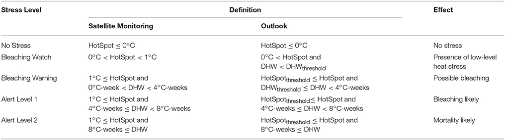
Table 1. Bleaching heat stress levels defined for CRW's satellite Bleaching Alert Area product, based on CRW's satellite HotSpot and DHW products, and CRW's Outlook Versions 3 and 4.

Model Prediction Metrics

CRW's Outlook systems (including Versions 3 and 4) first generate daily predictions of HotSpot and DHW at each lead-time ranging from 1-day (the day after the initial condition day) to 270-days, using daily CFSv2 SST predictions of each model run (ensemble member).

As in the satellite monitoring, the HotSpot prediction at a given grid cell on a particular day is calculated as the (positive) difference between the daily CFSv2 SST prediction and the Outlook MMM (re-centered MMM described in section CFSv2 SST Climatology) at the corresponding lead-time. The DHW prediction for the day accumulates 84 consecutive daily HotSpot predictions ending on the predicted date. The method of using the lead-time dependent MMM climatology to calculate HotSpots from the CFSv2 daily SST predictions of corresponding lead-times is consistent with the systematic error correction applied by Saha et al. (2014) and Zhang and van den Dool (2012) on the CFSv2 predictions.

For a daily DHW prediction with lead-times of up to 83-days, the DHW is computed as described above but using a combination of dOISSTv2-based and predicted HotSpots. The dOISSTv2-based daily HotSpot is the observed HotSpot, calculated as the anomaly between the dOISSTv2 and the dOISSTv2-based MMM (described in section dOISSTv2 SST Climatology); hence, the predicted daily DHW for lead-times <84-days accumulates both observed HotSpots and predicted HotSpots. The accumulation of dOISSTv2-based HotSpots into the DHW prediction applies CRW's satellite algorithm.

A modification from the satellite algorithm is required to account for differences between the model and satellite SSTs. Variability of the daily CFSv2 SST forecast within the top 10 m layer of the ocean was observed to be smaller than the variability in the top 1 m (X. Wu, pers. comm.), against which the satellite SST analysis is calibrated. Also, the upper meter of the ocean usually experiences significant diel variation during the low wind and clear sky conditions often present during bleaching events. The differences between the 10 and 1 m SST values can result in dampened daily SST excursion above the corresponding Outlook MMM climatologies. If the same high-pass filter (threshold) of 1°C, used in the satellite monitoring, were applied to filter daily HotSpot predictions at all lead-times, fewer predicted HotSpots at longer lead-times would be accumulated and the predicted DHW would be smaller than the observed satellite DHW. To relate the predicted DHW value to a bleaching risk level using the same classifications as in CRW's satellite algorithm (Table 1), while preserving the satellite HotSpot algorithm in calculating the predicted HotSpot, a HotSpot threshold that is <1°C is necessary for any predicted daily HotSpot. This is the approach applied in the previous and current versions of CRW's Outlook systems.

A lead-time dependent HotSpot threshold was originally developed for CRW's LIM-based, statistical seasonal Coral Bleaching Outlook system (Liu et al., 2009) and then adapted for the CFSv1-based Outlook Version 1 (Eakin et al., 2012). It was based on experiments that predicted spatial distributions and magnitudes of heat stress and compared those to CRW's satellite monitoring during various confirmed mass bleaching events, including the 2005 Caribbean-wide and the 2010 global bleaching events. Applying a uniform HotSpot threshold of 0°C caused overestimation in the DHW prediction for shorter lead-times, while a HotSpot threshold of 0°C was required for predicting sufficient heat stress for longer lead-times. The lead-time dependent HotSpot threshold used with the LIM-based outlook was hence adapted for Outlook Versions 3 and 4, with a minor adjustment.

Outlook Versions 3 and 4 apply a HotSpot threshold (HotSpot_threshold) that decreases linearly from 1°C at the lead-time of 0-days (i.e., the initial condition day) to 0°C at lead-times of 70-days (Day 70; i.e., the end of 10-weeks) and beyond (Figure 1; Table 1). This formula was chosen after testing various slopes with 1-week increments for a few known major bleaching events. For a predicted date, if the predicted HotSpot value reach the HotSpot_threshold for the corresponding lead-time, the HotSpot value is accumulated into the DHW prediction. Such conditions initiate at least a predicted Bleaching Warning for the date in question. However, modifying the HotSpot threshold required a lead-time dependent DHW threshold for categorizing heat stress as well. As the HotSpot_threshold decreases to zero by Day 70, any subsequent positive HotSpot value results in a DHW accumulation. If the satellite-based stress classification (Table 1) had been applied directly for those days, the Bleaching Watch level would have been skipped and the stress would have jumped directly from No Stress to Bleaching Warning. To prevent this from occurring, a linearly varying DHW threshold, DHW_threshold, was introduced (Figure 1). It started with 0°C-weeks at Day 0 and increased linearly to 2°C-weeks at Day 70 to maintain the Bleaching Watch level throughout the lead-times included in the Outlook. Note that the linear change in the HotSpot threshold over lead-times of 1–70-days was developed to allow sufficient daily predicted HotSpots to be accumulated into the DHW prediction while preventing too much DHW accumulation. This is not related to the DHW accumulation time period of 84-days. Other approaches may produce Outlook values with good or better matches with observed heat stress and will be tested for future versions.

FIGURE 1

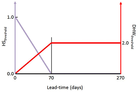
Figure 1. Schematic of lead-time dependent HotSpot threshold (HotSpot_threshold, purple) and Degree Heating Week (DHW) threshold (DHW_threshold, red) used in the algorithm for Outlook Versions 3 and 4.

Our most recent examinations, based on predictions made for the 2015 bleaching event in the Main Hawaiian Islands (MHI) and 2016 bleaching event in the northern Great Barrier Reef (GBR), further verified the application of lead-time dependent HotSpot and DHW thresholds. Note that published analyses of the CFSv2 (e.g., Xue et al., 2013; Saha et al., 2014) did not evaluate changes in variability of the CFSv2 SST over lead-times on daily or weekly bases.

Mass bleaching of corals across a reef usually takes weeks of stressful conditions to develop. CRW's Outlook, updated once a week, is not designed to provide guidance on the daily development of heat stress. Therefore, weekly predictions are derived from the daily predictions before further processing. Given that the HotSpot and DHW are positive-only variables, the medians of seven daily values of the HotSpot and DHW over a calendar week are used as the predictions for that week. The weekly Bleaching Alert Area prediction of an ensemble member is then determined from the weekly HotSpot and DHW predictions of that member, based on the stress classifications provided in Table 1. The weekly predictions are calculated for each ensemble member separately.

In CRW's Outlook system, a weekly time period covers Monday–Sunday and is tracked by Sunday's date. A weekly prediction with a lead-time of 1-week is for the week immediately following the initial condition week (defined below); weekly predictions are produced out to approximately 4-months.

Probabilistic Bleaching Outlook

Weekly Outlook

The weekly probabilistic Outlook for a week is constructed based on the weekly Bleaching Alert Area predictions from all the available ensemble members for the week. The Outlook Version 4 has been developed and replaced Version 3 in May 2017. The difference between the two versions is the number of CFSv2 daily runs used in the probabilistic Outlook, as described below.

Weekly Outlook Version 3

The probability of predicted stress was determined from the ensemble of model runs each week. In the Outlook Version 3, the 28 Bleaching Alert Area values (i.e., four runs per day over 7-days of the initial condition week), derived from the four 9-month CFSv2 SST runs daily, were pooled for each predicted week. A probabilistic forecast was then produced for each predicted week by determining the heat stress levels reached or exceeded by 10 specified percentages of ensemble members at each grid cell. The 10 pre-set probabilistic levels range from 10 to 100%, in increments of 10%. For example, the 90% probabilistic Outlook for a predicted week at a grid cell would be the stress level (Table 1) that 26 of the 28 ensemble members met or exceeded. The probability of each of four bleaching heat stress ranges (Watch and higher, Warning and higher, Alert Level 1 and higher, and Alert Level 2) also was determined from all available ensemble members for the week to form a full set of weekly probabilistic Outlook products.

Weekly Outlook Version 4

In the Outlook Version 4, all 16 daily runs, including the four 9-month runs used in the Outlook Version 3, as well as the other 12 daily runs with shorter forecast ranges, are incorporated. All 45-day and one-season runs initialized over a calendar week can consistently predict for at least 5 and 12-weeks, respectively, into the future. Pooling all available members for each week, the first 5-weeks in the prediction have 112 ensemble members; weeks 6–12 have 49 members; and weeks 13–37 have 28 members. The same algorithm used in the Version 3 is used to generate Version 4 of the probabilistic weekly Outlooks. The only difference comes from the varying number of ensemble members over the course of the 4-month time period. As in Version 3, for each predicted week, heat stress levels are determined for 10 pre-set probabilistic levels (from 10 to 100%, in increments of 10%) at each grid cell, along with the probabilities for the four stress ranges.

Although the Outlook Version 4 uses more ensemble members than the Outlook Version 3, initial comparisons have revealed that they are remarkably similar (not shown). This may indicate that the four 9-month control runs capture most of the variability found in the full set of runs. Versions 3 and 4 of the weekly Outlooks are identical for Week 13 and longer lead-times.

Four-Month Outlook

CRW's probabilistic 4-Month Outlook is constructed from the weekly Outlooks described above. A period of 4-months is the approximate length of a bleaching season (warm season) on most coral reefs. The 4-month period of the Outlook starts with the second predicted week (lead-time of 2-weeks), and Sunday's date determines the first month. The Outlook period ends on the last Sunday of the fourth month. Weekly Outlooks ranging from a lead-time of 2-weeks to at least 15-weeks and up to 20-weeks (depending on the lead-time of the last Sunday in the fourth month) are used to derive the 4-Month Outlook. The weekly Outlook with 1-week lead-time is excluded, as the 4-Month Outlook is updated weekly in the middle of that week.

For each of the 10 predetermined probabilistic levels (from 10 to 100%, in increments of 10%) used in the weekly Outlooks, the maximum temporal composite over the 4-month period is created by extracting the maximum values from all of the weekly Outlooks with the corresponding probabilistic level. The resulting 10 4-month maximum composites are the probabilistic 4-Month Outlooks for the corresponding probabilistic levels. For each of the four stress ranges, the probabilistic 4-Month Outlook provides the highest weekly probability predicted among all of the weekly Outlooks during a 4-month period.

Product Availability

Global and regional maps of the most recent update of the probabilistic 4-Month Outlook at 90% and 60% probabilities (Figures 2A,B for Version 3, respectively) are posted on CRW's website at https://coralreefwatch.noaa.gov. These are updated weekly, along with the weekly Outlooks of the corresponding probabilities. Four probabilistic maps showing the percentage of ensemble members reaching the four heat stress ranges (Alert Level 2, Alert Level 1 and higher, Bleaching Warning and higher, and Bleaching Watch and higher) also are displayed (Figures 2C–F for Version 3, respectively).

FIGURE 2

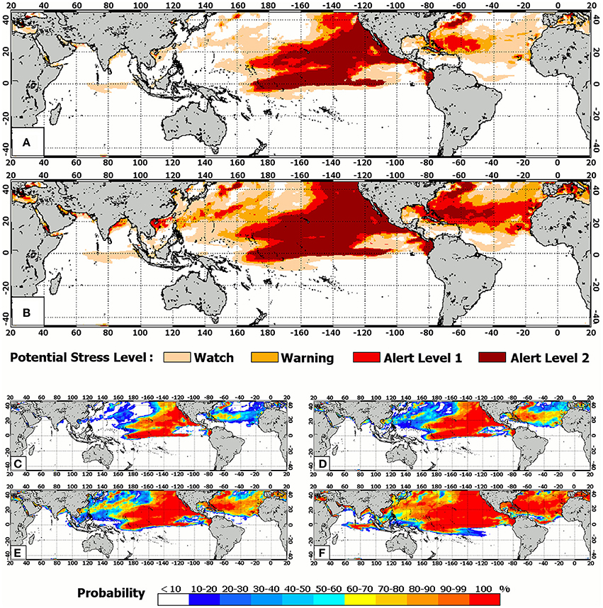
Figure 2. CRW's probabilistic 4-Month Coral Bleaching Outlook Version 3 issued on July 7, 2015 for July–October 2015: stress levels with (A) 90% and (B) 60% probabilities; probabilities for (C) Alert Level 2, (D) Alert Level 1 and higher, (E) Warning and higher, and (F) Watch and higher. Note that the Outlook was derived for each grid cell in the maps regardless of the existence of shallow-water coral reefs at that specified grid cell.

Given that the daily runs need to be collected over a calendar week to form an ensemble system, the Outlook is run and products are updated weekly. This occurs every Tuesday at approximately 19:00 Z, when all of the daily CFSv2 SST predictions produced during the previous week (through Sunday) become available to CRW. The Outlooks are publicly available via CRW's website: https://coralreefwatch.noaa.gov.

The very first runs of the CFSv2 SST forecast were run using initial conditions from April 1, 2011, so the earliest week producing a complete set of 7-day CFSv2 runs was the week ending on April 10, 2011. Thus, the first predicted week ended on April 17, 2011 and the earliest 4-Month Outlook Versions 3 and 4 were for the period April-July 2011.

Performance of Outlook Version 3

CFSv2 SST Skill

The skill analysis of the CFSv2 SST was discussed by Saha et al. (2014), Xue et al. (2013), and Zhang and van den Dool (2012), among others. A set of CFSv2 SST skill maps showing the correlation and Root Mean Square Error (RMSE) of the SST hindcasts, as compared with the dOISSTv2 SST (Reynolds et al., 2002), is accessible at: http://www.cpc.ncep.noaa.gov/products/people/mchen/CFSv2HCST/metrics/rmseCorl.html. A subset of the correlation maps that are relevant to CRW's Outlook is reproduced in Figure 3 using the matching color scale. The correlation maps are for the daily SST hindcasts of 1982–2009. The maps of 0-month lead-time are for the 3-month period immediately after the initial condition month; the maps of 1-month lead-time are for the 3-month period starting with the second month after the initial condition month. Given that CRW's Outlook covers a period of up to four months, only the lead-times of 0- and 1-month, together covering four months after the initial condition month, are relevant. The CFSv2 SST skill depends on both the month predicted and lead-time. The skill for most of the global tropical oceans, particularly areas where corals live (Figure 4A), was high (correlation > 0.7 and RMSE <0.6°C; see the CFSv2 SST skill website mentioned above for RMSE) for both lead-times of 0- and 1-month. As a result, it was expected that for most of the global tropical regions, the daily CFSv2 SST predictions would produce a skillful 4-Month Coral Bleaching Outlook.

FIGURE 3

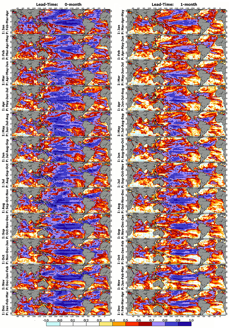
Figure 3. Correlations between 1982–2009 daily CFSv2 SST hindcasts and dOISSTv2 SSTs for 12 initial condition months (rows, January–December) and lead-times of 0- (left column) and 1-month (right column). I: initial condition month; P: predicted 3-month period. Images reproduced from NOAA's CFSv2 website.

FIGURE 4

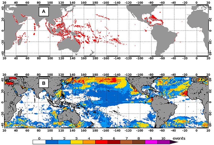
Figure 4. (A) Map of tropical coral reef locations; (B) Numbers of observed bleaching events identified by CRW's 50 km satellite monitoring during the comparison time period of August 1, 2011–December 27, 2015.

A map of global tropical coral reef locations is provided in Figure 4A as a reference for discussing CFSv2 SST and Outlook skills. Global coral reef locations were compiled by CRW from several data sources (Heron et al., 2016b); the multi-source compilation by the United Nations Environment Programme–World Conservation Monitoring Centre (UNEP-WCMC) and the WorldFish Centre, in collaboration with the World Resources Institute (WRI) and The Nature Conservancy (TNC) (UNEP-WCMC WorldFish Centre, 2010), includes the Millennium Coral Reef Mapping Project and the World Atlas of Coral Reefs. This was augmented using other local marine atlases (e.g., UNEP/IUCN, 1988a,b) and direct communication with researchers (i.e., where reef observation surveys had been reported).

We further examined SST skill for the bleaching season of major coral reef regions globally. For example, the SST hindcasts initialized in June were high in skill (r > 0.7) for predicting both the July-August-September (0-month lead-time) and August-September-October (1-month lead-time) periods for most of the tropical oceans. These months are during the bleaching season for reefs of the Hawaiian archipelago, the Marshall Islands, Japan, the Caribbean, and Florida (Heron et al., 2016a), among other regions. The SST hindcasts initialized in February, March and April were high in skill (r > 0.7) for predicting 1-month lead time periods of April-May-June, May-June-July, and June-July-August, respectively, which are the bleaching seasons in Indonesia, Malaysia, Thailand, Guam and the CNMI (Heron et al., 2016a), among other coral reef areas. However, the skill of SST hindcasts for the Great Barrier Reef (GBR)'s peak bleaching season (February-March-April) did not reach 0.7 for most of the region. The reason for relatively lower SST prediction skill in the GBR will require further investigation.

Outlook Skill

A limited analysis of the Outlook's performance was carried out by comparing predicted bleaching events with heat stress events identified by CRW's operational 50 km satellite bleaching heat stress monitoring (Liu et al., 2013; https://coralreefwatch.noaa.gov). The 50 km satellite products started in late 2000 (Liu et al., 2013) and continued until January 2016, when the original satellite SST analysis was discontinued and replaced (see Heron et al., 2014). Hence, the satellite data available for the evaluation were for 2001–2015. A more complete evaluation is planned using CRW's new CoralTemp 5 km dataset from 1985-present once available in 2018.

The skill analysis discussed here is for the Outlook Version 3 only. It was based on weekly Outlooks with lead-times ranging from two to at least 15-weeks and up to 20-weeks. Hence, the analyses were conducted on the weekly Outlooks for lead-times of 3, 5, 9, 13, and 17-weeks; these approximate to the beginning weeks of the half, one, two, three, and 4-months into the future. As noted above, the earliest available initial condition week for Version 3 was April 10, 2011; therefore, the first predicted weeks available for the five lead-times were May 1, May 15, June 12, July 10, and August 7, 2011, respectively. The common predicted time period by all five lead-times was chosen for the skill analysis; i.e., August 1, 2011 (the Monday of the week ending on August 7) through December 27, 2015 (the last Sunday of 2015). For each specified lead-time, all of its weekly Outlooks were extracted to form a time series. Then, in each of the five time series, predicted bleaching events (see the definition of bleaching event below) were compared with bleaching events observed by satellite monitoring over the same period to produce hit, miss, and false alarm analyses.

Although both the satellite Bleaching Alert Area and modeled Outlook had the same spatial resolution, their grid cell layouts were a half grid cell off in both zonal and meridional directions. As a result, both were resized to a 0.25° grid cell layout by dividing every original 0.5° grid cell uniformly into four 0.25° grid cells that were assigned the same value as the original grid cell; the comparison was carried out at co-located 0.25° grid cells.

Two types of events were defined for this analysis: heat stress events and bleaching events. A bleaching event was recorded as the presence of Alert Levels 1 and/or 2, both of which are associated with at least significant bleaching (Table 1). A heat stress event was recorded as the presence of stress at or greater than Bleaching Warning. Hence, any bleaching event was contained in a heat stress event, but a heat stress event did not necessarily contain a bleaching event. The beginning day of a heat stress event was set on the first day on which a Bleaching Warning appeared; the beginning day of a bleaching event was set on the first day on which Alert Level 1 or 2 appeared. A heat stress event ended when the stress decreased to a level below Bleaching Warning (i.e., No Stress or Bleaching Watch) and remained there for at least 84-days. The ending day of a bleaching event was set on the last day when Alert Level 1 or 2 was experienced within a heat stress event. 84-days is the duration of the DHW accumulation. CRW's satellite data indicated that at some equatorial locations, in some years, heat stress did not decrease to a level of No Stress or did not remain at No Stress for up to 84-days before a new bleaching event started. Also, a grid cell could have a long period of time experiencing heat stress at the Bleaching Warning level with only a short burst of Alert Level 1 or 2, as short as one twice-weekly period. This still would be classified as a bleaching event. Similar situations occurred in the Outlook. In cases when a heat stress event and/or bleaching event existed on the first day of an examined time period, the corresponding event beginning date was recorded as of that day, although the event may have started well before the first predicted week. The predicted bleaching events (not heat stress events) were compared with satellite detected bleaching events. Hereafter, a bleaching event identified by the satellite monitoring is referred to as an observed bleaching event or observed event. As this is a test of the skill in predicting the heat stress that causes bleaching, the Outlook is only compared with heat stress data and not field observations of bleaching. Finally, CRW uses the Outlook of 60% probability to issue warnings of impending bleaching; therefore, the performance of the 60% probability Outlook is discussed herein.

The temporal resolution of the 50 km satellite Bleaching Alert Area was twice-a-week, based on a repeated Monday–Wednesday (3-days) and Thursday–Sunday (4-days) SST analysis cycle. The beginning and end dates of an event were the first and last date of the corresponding twice-a-week periods, respectively. The Outlook had a weekly temporal resolution (Monday–Sunday), so the beginning and end dates of a predicted event were the Monday and Sunday of the corresponding weeks, respectively. Given that the heat stress level is based on accumulated stress over 84 consecutive days, any potential offset by half a week in the event beginning and end dates between the satellite monitoring and Outlook can be ignored.

Hits, misses, and false alarms by the Outlook were counted at each grid cell, and compared with observed bleaching events (determined by their beginning and end dates), for each of the five lead-times over the same comparison time period. For each observed event, overlapping predicted events were searched for, regardless of event duration and the relative beginning and end dates. Any predicted event that overlapped an observed event was a hit. If an observed event was not overlapped by a predicted event, a miss was counted. If a predicted event did not overlap any observed event, a false alarm was registered.

The number of observed events identified for each grid cell for the comparison time period is plotted in Figure 4B; the corresponding numbers of predicted events for examined lead-times are plotted in Figure 5. Among all the grid cells, the maximum number of observed events was six, and the maximum numbers of predicted events were six, eight, seven, seven, and eight for the lead-times of 3, 5, 9, 13, and 17-weeks, respectively (Table 2).

FIGURE 5

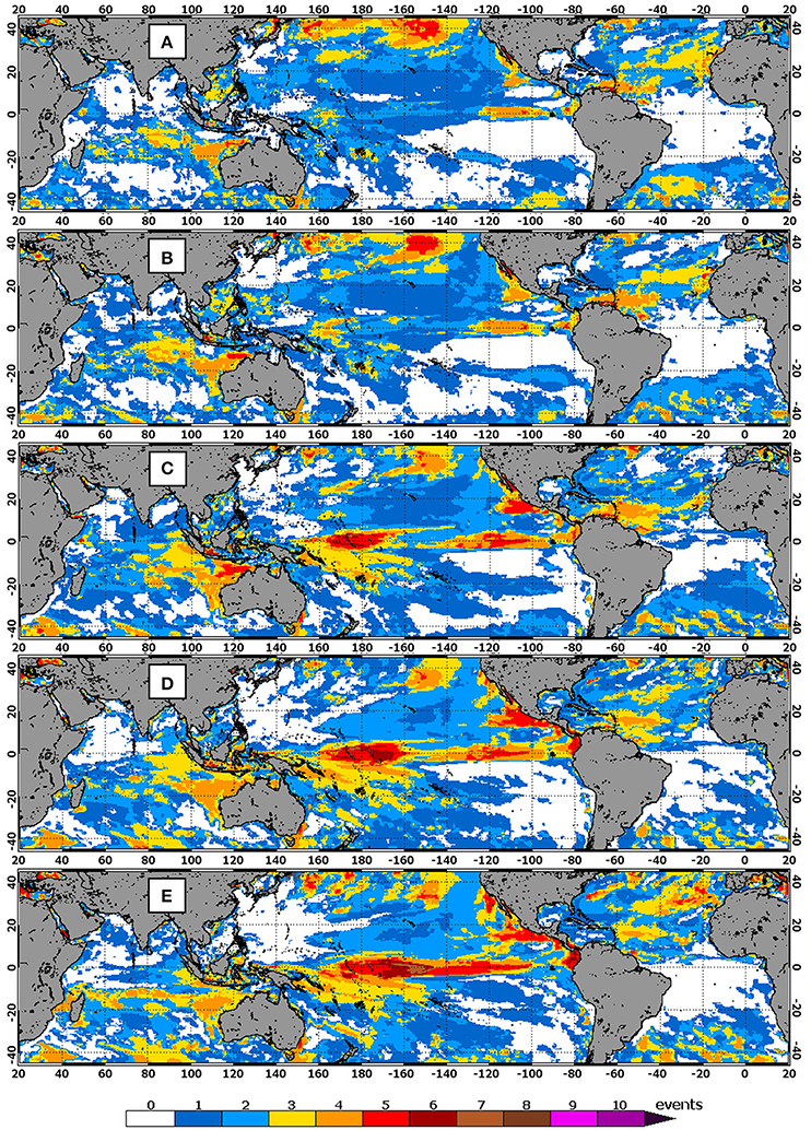
Figure 5. Numbers of bleaching events identified by CRW's weekly Outlooks (Version 3) of 60% probability during the comparison time period of August 1, 2011–December 27, 2015 for lead-times of: (A) 3-weeks, (B) 5-weeks, (C) 9-weeks, (D) 13-weeks, and (E) 17-weeks.

TABLE 2

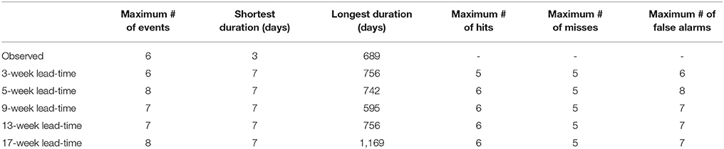
Table 2. The maximum numbers of observed and predicted bleaching events, their shortest and longest event durations, and the maximum counts of hits, misses, and false alarms of the Outlook, among all grid cells, for lead-times of 3, 5, 9, 13, and 17-weeks, during the comparison time period of August 1, 2011–December 27, 2015.

Given that there were at most six observed events at a grid cell (Table 2) and a good percentage of grid cells did not have any observed events, calculating rates of hit, miss, and false alarm could not provide normally-distributed data to quantitatively analyze skill. A longer time series of Outlook data (beyond 2011–2015) will be needed to conduct a fully quantitative skill analysis. Hence, hit, miss, and false alarm counts, instead of their rates and other derived skill indices, are presented in Figures 6–8, respectively. The maximum counts of hit, miss, and false alarm among all grid cells for each of the five lead-times are provided in Table 2. For regions with a count of zero for hit, miss, and false alarm, the Outlook was successful in not predicting a bleaching event at the corresponding lead-times.

FIGURE 6

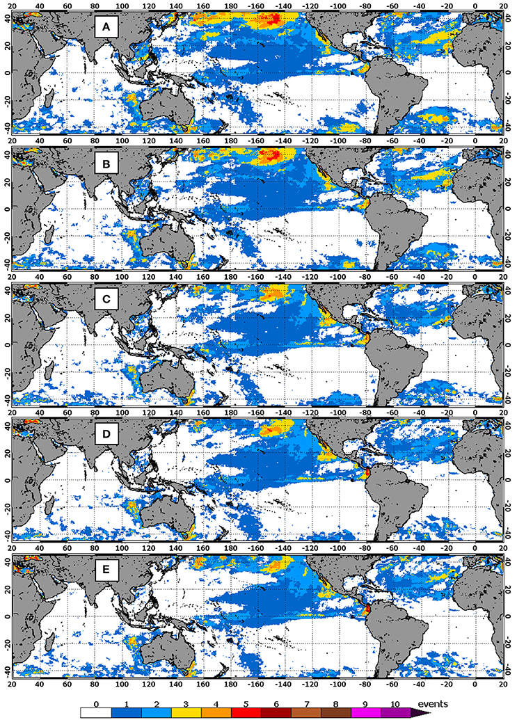
Figure 6. Numbers of hits by CRW's weekly Outlooks (Version 3) of 60% probability during the comparison time period of August 1, 2011–December 27, 2015 for lead-times of: (A) 3-weeks, (B) 5-weeks, (C) 9-weeks, (D) 13-weeks, and (E) 17-weeks.

Figures 6 (hit), 7 (miss) show that throughout the lead-times, the Outlook performed well in predicting observed bleaching events for most coral reef regions for up to 4-months into the future. Exceptions to this were areas such as the northern Philippines, South China Sea, and Timor Sea, where miss counts were mostly up to four, especially at longer lead-times (Figure 7). At the 17-week lead-time, the Outlook missed some observed events in the Northwestern Hawaiian Islands (NWHI) and in the eastern Caribbean (Figure 7E). Numbers of misses at each lead-time were low across most equatorial regions (Figure 7).

FIGURE 7

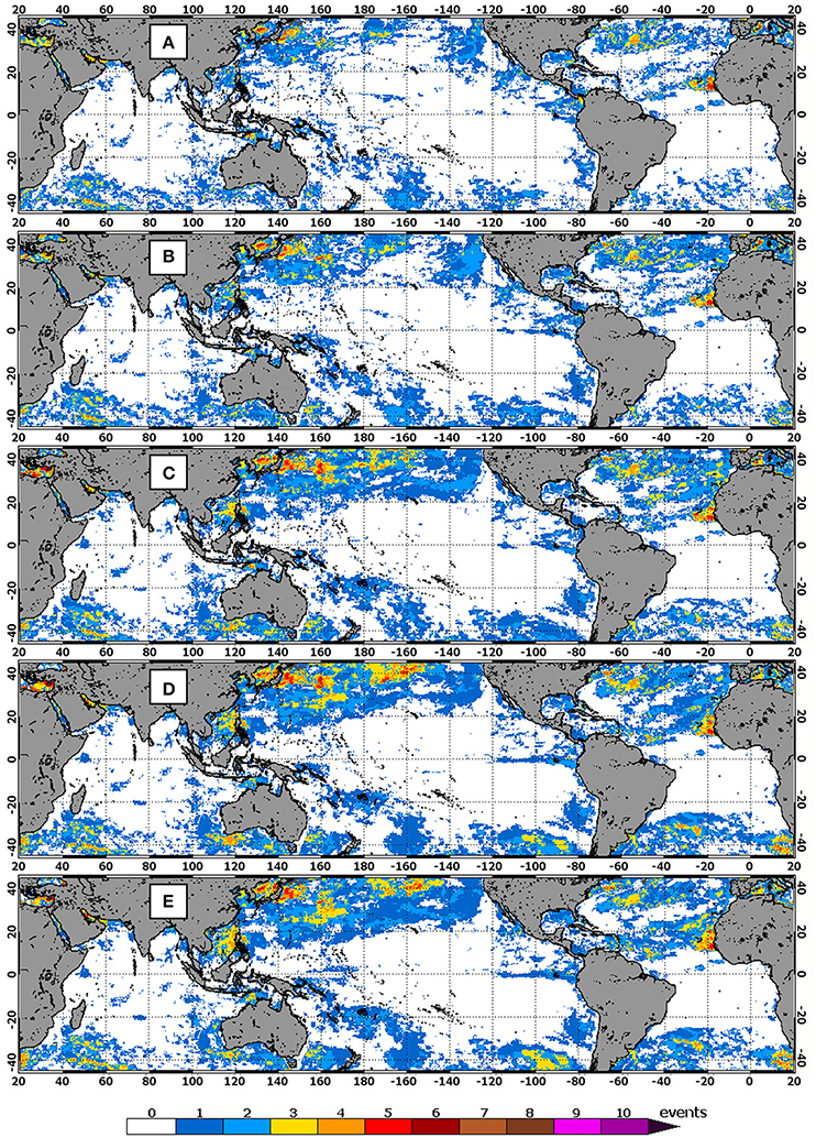
Figure 7. Numbers of misses by CRW's weekly Outlooks (Version 3) of 60% probability during the comparison time period of August 1, 2011–December 27, 2015 for lead-times of: (A) 3-weeks, (B) 5-weeks, (C) 9-weeks, (D) 13-weeks, and (E) 17-weeks.

The false alarm is another critical aspect of the skill analysis. At short lead-times of 3 and 5-weeks, the false alarm count was relatively high in the eastern equatorial Pacific, southeastern Caribbean, off the Northern Territory of Australia, in parts of southern Indonesia, and in the central Indian Ocean (Figures 8A,B). Areas with higher false alarm counts expanded spatially at the longer lead-time of 9-weeks to include portions of the western equatorial Pacific Ocean (Figures 8C,D). At the lead-time of 17-weeks, the false alarm count decreased in the eastern Indian Ocean and the Caribbean but increased in the central and western equatorial Pacific Ocean and western Indian Ocean (Figure 8E). Over-prediction may have been caused by highly variable and short-lived weather events, especially tropical storms and shifts in the monsoon, which are not predictable by seasonal-scale climate forecast systems. Tropical storms can relieve heat stress that otherwise would have caused severe bleaching (Manzello et al., 2007; Hughes et al., 2017). Detailed discussion of extreme weather event impacts is outside the scope of this paper. The decrease in the HotSpot threshold with increasing lead-time may have contributed to some false alarms. Regions identified with relatively high miss and false alarm counts will be investigated further once longer time series of satellite and modeled data are available for an appropriate comparison. For the regions with a tendency toward false alarm, prediction of upcoming bleaching events, especially at longer lead-times, should be treated cautiously in making management decisions. The predictions may be useful to guide early preparation but should be further informed by viewing CRW's near real-time satellite monitoring.

FIGURE 8

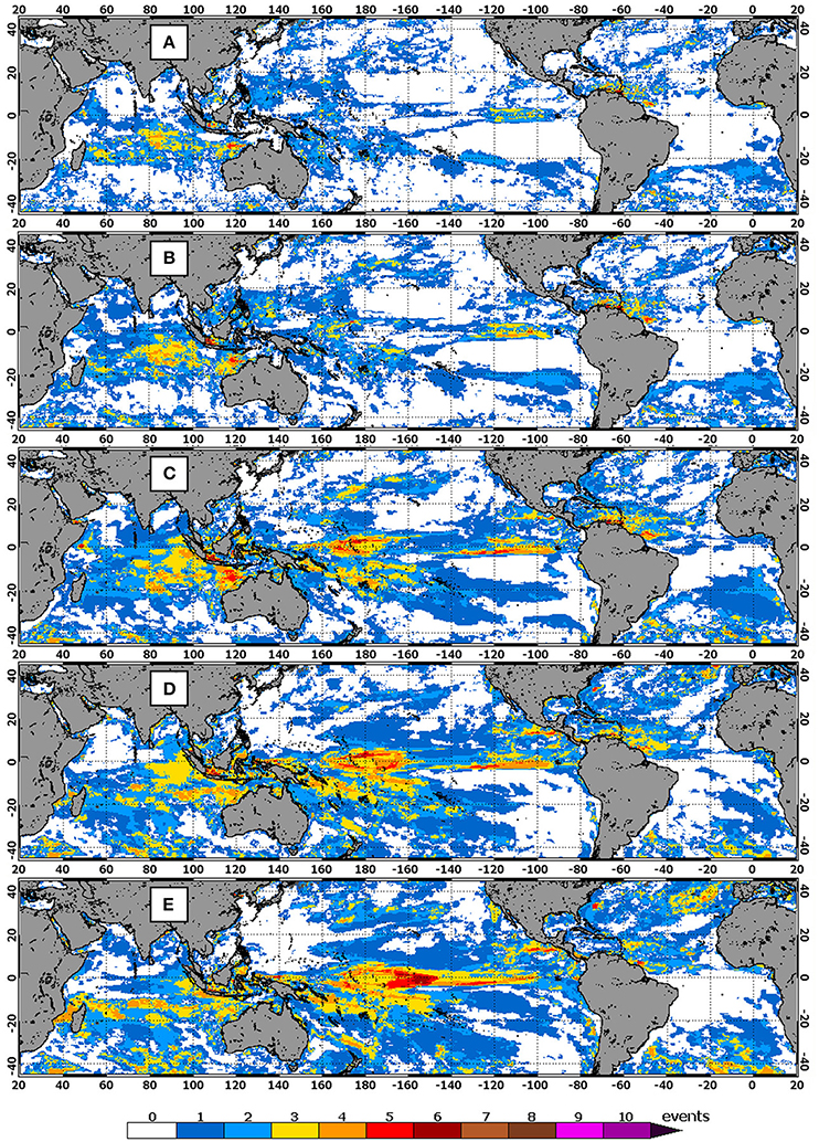
Figure 8. Numbers of false alarms by CRW's weekly Outlooks (Version 3) of 60% probability during the comparison time period of August 1, 2011–December 27, 2015 for lead-times of: (A) 3-weeks, (B) 5-weeks, (C) 9-weeks, (D) 13-weeks, and (E) 17-weeks.

In this evaluation, counts of hit, miss, and false alarm did not take into account the duration of the bleaching event, only the presence and absence of overlaps between observed and predicted events. Multiple observed events may have overlapped one predicted event, and vice versa. Refined analyses taking into account event duration will be conducted when a longer data time series becomes available. As an example, maps of the shortest and longest durations of the predicted bleaching events for the 5-week lead-time and the corresponding observed bleaching events are provided in Figure 9 to demonstrate that the Outlook was compatible with the satellite observations in terms of spatial distribution and range of event duration. Table 2 also lists the ranges of event duration for the five lead-times.

FIGURE 9

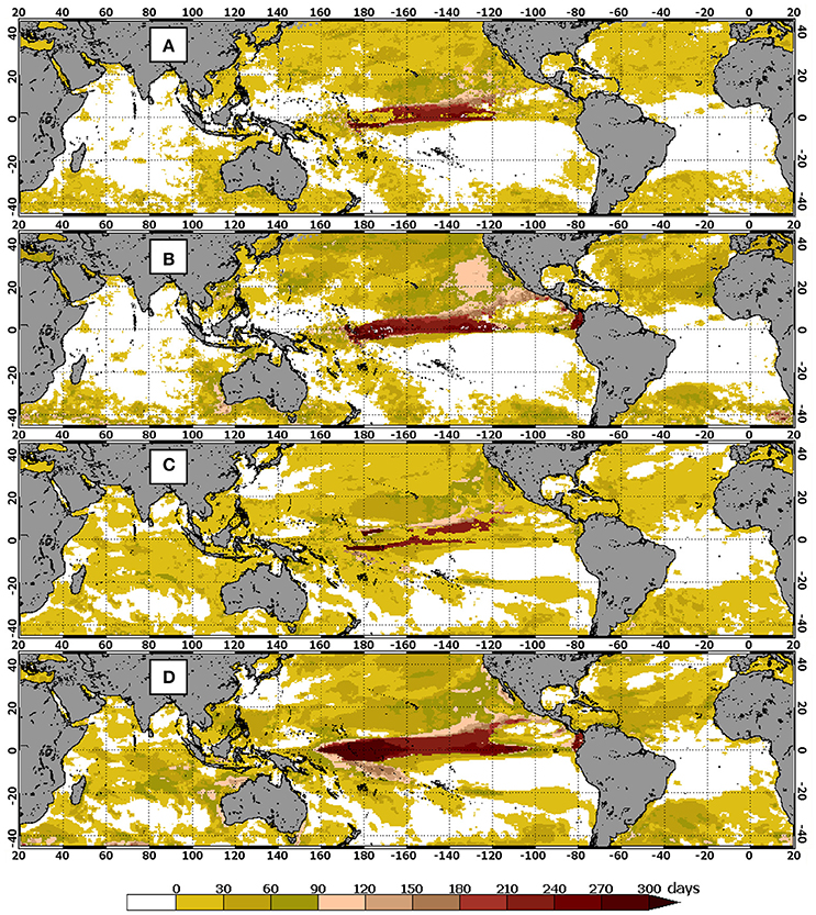
Figure 9. The shortest (A) and longest (B) event durations identified by CRW's 50 km satellite monitoring and the shortest (C) and longest (D) event durations predicted by CRW's weekly Outlooks (Version 3) of 60% probability with a lead-time of 5-weeks during August 1, 2011–December 27, 2015.

As the hindcasts were run on 1-day out of every five (as described earlier) and the real-time version of the CFSv2 runs every day, the ensemble system has to be revised to accommodate the lower number of weekly ensemble members in the hindcast. Given that the focus of this manuscript is on the algorithm, we plan to analyze the Outlook hindcast results and associated skill analysis for publication in a separate article.

Application of CRW's Outlook in Predicting the Third Global Coral Bleaching Event

The third global coral bleaching event started in the CNMI and Guam in June 2014 and was declared global in its extent by NOAA in October 2015 after widespread bleaching had been reported in the Pacific, Atlantic, and Indian Ocean basins (NOAA News Release, 2015; Eakin et al., 2017). The extremely strong 2015–2016 El Niño further spread and worsened the global event in 2016 (Normile, 2016; Eakin et al., 2017). By February 2016, it was the longest global event ever recorded (NOAA News Release, 2016a) and in June 2016 was projected to become a continuous 3-year event (NOAA News Release, 2016b). This event affected more reefs in the U.S. and worldwide than either previously documented global bleaching event (1998 and 2010; Eakin et al., 2017). It has been the worst ever in some locations [e.g., the northern GBR (Hughes et al., 2017), Kiritimati Island (The Washington Post, 2016), Jarvis Island (Brainard et al., 2018), and the NWHI (Couch et al., 2017)]. Some reefs bleached extensively for the first time on record (e.g., the northern GBR; Hughes et al., 2017), and some reefs were affected in consecutive years [e.g., Hawaii, the Florida Keys (Eakin et al., 2017), and the CNMI (Heron et al., 2016b)].

CRW's Outlook and its near real-time satellite products predicted, monitored, and tracked this multi-year global bleaching event starting well before it began. They were used for management preparedness and response: e.g., governmental closures of major dive sites in anticipation of extensive coral bleaching (e.g., The Guardian, 2016) and changes in location and resource allocation for in-water monitoring and ecological impact surveys (e.g., Heron et al., 2016b; Eakin et al., 2017). Figure 10, based on CRW's daily global 5 km satellite monitoring (Liu et al., 2014; https://coralreefwatch.noaa.gov), shows the highest heat stress levels reached during June 2014–May 2017. The 5 km products are CRW's next-generation satellite products; in early 2016, they replaced CRW's heritage 50 km products as the core component of CRW's decision support system for coral bleaching management (Heron et al., 2016b; Liu et al., 2017). In the figure, ellipses outline those reef regions where CRW's 5 km products indicated bleaching should be occurring and where field partners and users had reported extensive bleaching. CRW is still actively collating observations of coral bleaching and no bleaching from the field. Analysis of this global bleaching event and the performance of CRW's satellite and Outlook products during the event will be conducted and published soon.

FIGURE 10

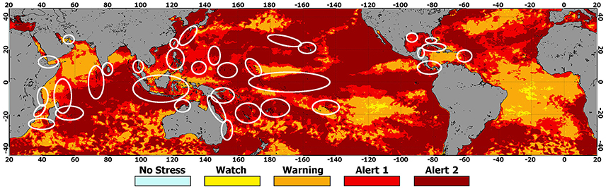
Figure 10. Maximum composite of CRW's daily global 5 km satellite Bleaching Alert Area (Version 3) for June 2014–May 2017. Major bleaching has been reported to CRW by resource managers, scientists, and the public in the coral reef regions outlined by ellipses.

Following the timeline of the third global bleaching event, the application of CRW's Outlook to predict some key phases of the event is described herein. The Outlook issued on June 24, 2014 (Figure 11A) predicted imminent bleaching in the CNMI and Guam that would start early that month (weekly Outlooks are not shown but are accessible on the CRW website). This marked the onset of the third global bleaching event. Subsequent Outlooks (accessible on the CRW website), updated weekly, continued to predict the presence of Alert Level 1 or 2 in the region until late September 2014. This was confirmed by CRW's satellite monitoring at 50 km and 5 km resolutions. The 50 km satellite monitoring, for example, showed that Alert Levels 1 and 2 occurred in the region from early July (Figures 11B, 12B) through late September 2014, as confirmed by field observations (Heron et al., 2016b).

FIGURE 11

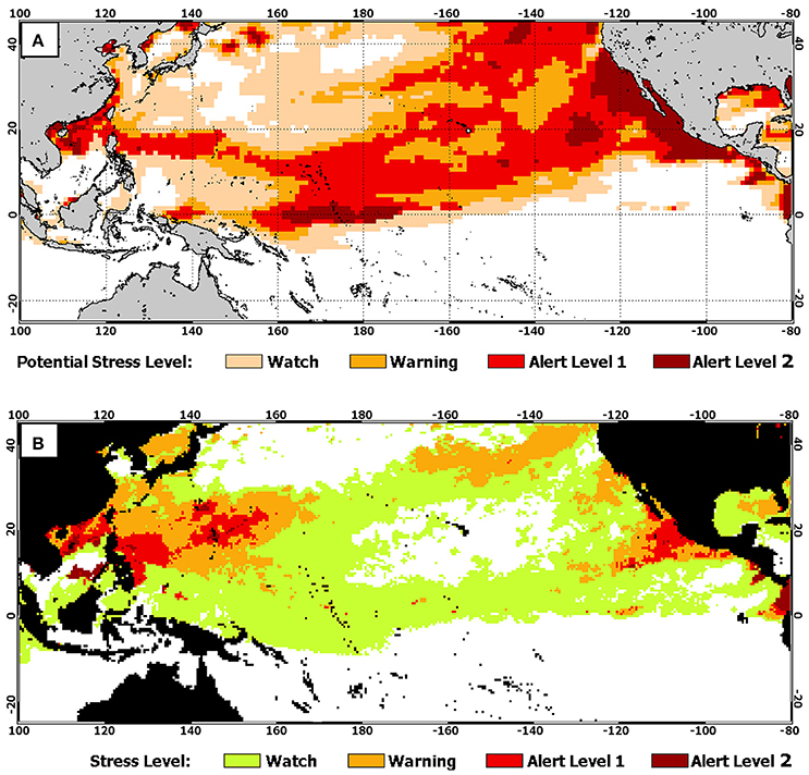
Figure 11. CRW's (A) 4-Month Outlook (Version 3) of 60% probability issued on June 24, 2014 for July–October 2014, predicting Alert Level 1 in the Commonwealth of the Northern Mariana Islands (CNMI), Guam, and the Main Hawaiian Islands (MHI), and the (B) monthly maximum 50 km satellite Bleaching Alert Area for July 2014, observing Alert Levels 1 and 2 in the CNMI.

FIGURE 12

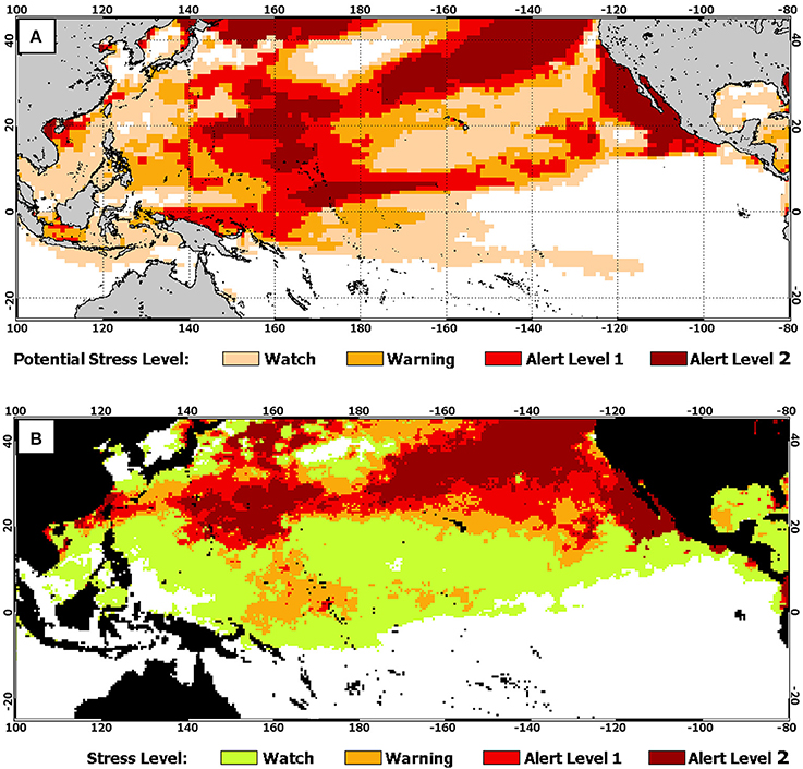
Figure 12. CRW's (A) 4-Month Outlook (Version 3) of 60% probability issued on August 26, 2014 for September–December 2014, predicting Alert Levels 1 and 2 in the Northwestern Hawaiian Islands (NWHI), and the (B) monthly maximum 50 km satellite Bleaching Alert Area for September 2014, observing Alert Levels 1 and 2 in the NWHI and the CNMI.

Four-Month Outlooks issued in June (Figure 11A), August (Figure 12A), and September 2014 (not shown) indicated the potential for Alert Levels 1 and 2 across the Hawaiian archipelago, especially in the NWHI in late 2014. These were confirmed by CRW's satellite monitoring (Figure 12B) and field observations, indicating widespread bleaching, with the middle section of the NWHI experiencing unprecedented mass bleaching (Bahr et al., 2015; Couch et al., 2017; Eakin et al., 2017).

As early as June 23, 2015, CRW predicted potential mass bleaching (https://coralreefwatch.noaa.gov) that later occurred in the MHI in summer/fall 2015; the Outlook issued on July 7, 2015 (Figure 13A) showed the spatial extent of Alert Level 2 that would be realized. CRW's satellite monitoring pinpointed the bleaching event in the Hawaiian archipelago, especially in the MHI, as lasting from August through October 2015 (Figure 13B) – as predicted by the Outlook. Concerned over CRW's Outlooks and near real-time satellite monitoring, the “Eyes of the Reef” volunteer reporting network held its first state-wide Bleach Watch “Bleachapalooza” monitoring event on October 3, 2015 (Hawaii Department of Land and Natural Resources, 2015)¹; this is the critical first tier of the Hawaii Department of Land and Natural Resources' Rapid Response Contingency Plan. It turned out to be an unprecedented, widespread, severe bleaching event in the MHI (Eakin et al., 2017). Based on CRW's Outlook, the Hawaii Division of Aquatic Resources collected specimens of rare corals to preserve them in onshore nurseries in case the mortality was severe. One of these species can no longer be found living on the reefs in Oahu; its genotypes are now found only in the nursery specimens (D. Gulko, pers. comm.).

FIGURE 13

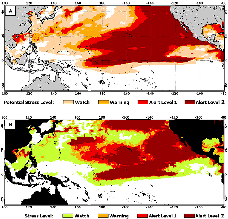
Figure 13. CRW's (A) 4-Month Outlook (Version 3) of 60% probability issued on July 7, 2015 for July–October 2015, predicting Alert Level 2 at the southeast end of the NWHI and in the Main Hawaiian Islands (MHI) during summer/fall 2015, and the (B) monthly maximum 50 km satellite Bleaching Alert Area for September 2015, observing Alert Level 2 in the same region.

In October 2015, NOAA officially declared the third global coral bleaching event (NOAA News Release, 2015), based on CRW's satellite monitoring and reported bleaching throughout the Pacific, Indian, and Atlantic Oceans. Based on CRW's Outlook of October 6, 2015 for October 2015–January 2016 (https://coralreefwatch.noaa.gov), the news release further indicated that the event would continue in the weeks and months ahead, affecting at least the Caribbean and central equatorial Pacific Ocean.

As early as December 1, 2015, CRW's Outlook predicted a mass bleaching event on the GBR during its summer season (February–April) 2016 (Figure 14A). That event turned out to be the worst in the GBR's history, especially in the northernmost portion of the GBR, where severe and widespread coral die-off was observed (e.g., Hughes et al., 2017). The December 1, 2015 Outlook also predicted the bimodal distribution of warm water (both in the northern GBR and New South Wales) that was eventually observed. Severe bleaching also was reported in and around Sydney Harbor (The ABC, 2016). Prior to peak bleaching, Thailand used CRW's prediction of severe heat stress to close numerous coral reefs to tourism as a way to reduce further stress to the reefs (The Guardian, 2016).

FIGURE 14

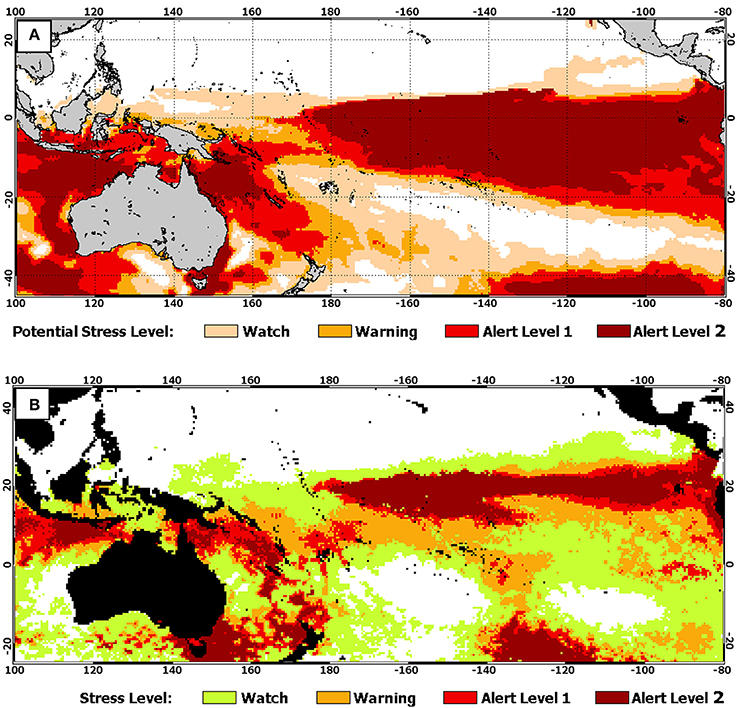
Figure 14. CRW's (A) 4-Month Outlook (Version 3) of 60% probability issued on December 1, 2015 for December 2015–March 2016, predicting Alert Levels 1 and 2 on the Great Barrier Reef (GBR) and in the waters off southeast Australia during the region's 2016 summer, and the (B) monthly maximum 50 km satellite Bleaching Alert Area for March 2015, observing Alert Levels 1 and 2 in the regions.

Kiritimati and Jarvis Islands, among other isolated islands and atolls in the central equatorial Pacific Ocean, were at the epicenter of the extremely strong 2015-16 El Niño. As predicted by CRW's Outlook (Figures 13–15) and confirmed by CRW's 5 km and 50 km satellite monitoring (Figures 10, 13, 14), Alert Level 2 bleaching heat stress lasted from May 2015 through May 2016 at some reef locations in the region. Once among the world's lushest coral reef ecosystems, the third global bleaching event killed most corals on these reefs (Associated Press, 2016a,b; NOAA Fisheries News Release, 2016; The Washington Post, 2016).

FIGURE 15

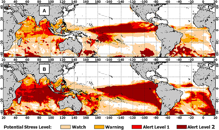
Figure 15. CRW's 4-Month Outlook (Version 3) of 60% probability (A) issued on March 3, 2015 for March-June 2015 and (B) on February 2, 2016 for February–May 2016. Long-lasting, continuous Alert Level 2 heat stress was predicted over islands and atolls in the central equatorial Pacific Ocean, including Kiritimati and Jarvis Islands, located at the epicenter of the extremely strong 2015-16 El Niño.

When the third global bleaching event ended its second year in mid-2016, NOAA again used CRW's Outlook to project the third year of the global event (NOAA News Release, 2016b). The global event continued into mid-2017 with bleaching predicted by CRW's Outlook (https://coralreefwatch.noaa.gov) and observed in-water in Fiji, Niue, American Samoa, and at scattered locations along the GBR (i.e., Eakin et al., 2017; The Guardian, 2017).

Concluding Remarks

CRW's probabilistic 4-Month Coral Bleaching Outlook system (https://coralreefwatch.noaa.gov) is the first and only freely available global system for predicting the heat stress that leads to mass coral bleaching.

As with any model predictions, improving forecast skill is always a challenge and remains a focus of CRW's ongoing development efforts. While we anticipate that improved versions of NOAA's CFS will become available within the next few years to enhance CRW's Outlook system and benefit the global coral reef community, CRW also will continue to work on refining the Outlook algorithm to enhance prediction skill across the global tropical oceans. The analysis presented in this study will guide future quantitative analyses and development and improvement of the Outlook system.

The recent release of Version 3 of CRW's daily, global 5 km satellite coral bleaching heat stress monitoring product suite significantly improved near real-time monitoring accuracy (C.M. Eakin, and G. Liu, pers. comm.). This version of the daily satellite HotSpot will replace dOISSTv2-based HotSpots in the Outlook system Version 5. Any advance in the satellite monitoring algorithm also will be applied in future versions of the Outlook.

A longer time series of Outlook hindcasts will be developed from the 1982–2010 CFSv2 SST hindcast run for a more complete and in-depth skill analysis. The results will be used to improve the Outlook algorithm and for guiding regional application of the Outlook. In addition, a new, longer CRW SST dataset, CoralTemp, will be released shortly. This 1985-present 5 km dataset will be instrumental in conducting a full skill analysis of the Outlook.

The CFSv2 SST exhibits low prediction skills for longer lead-times in many regions, as shown earlier. This contributes to the significantly varying skills in the Outlook. We will evaluate the feasibility of improving Outlook performance at regional scales. Furthermore, recent research has demonstrated the potential of using multi-model ensembles (MME) to improve seasonal prediction (e.g., Kirtman et al., 2014). The use of such MMEs in the Outlook also will be explored.

The Outlook already has provided critical warning to coral reef managers, scientists, and decision makers around the world to guide the management, monitoring, and protection of coral reefs. As an integrated component of CRW's global decision support system for coral bleaching management, the Outlook, together with CRW's satellite coral bleaching heat stress monitoring, has been extremely useful in forecasting and nowcasting the progression of the third global bleaching event from June 2014–May 2017. These CRW products have been incorporated into numerous bleaching preparedness and response plans, bleaching conditions bulletins and newsletters, and other documents and outreach materials established and distributed by coral reef managers and scientists around the globe.

Author Contributions

GL, CE, MC, and AK designed the study. GL and MC developed the products. GL, JD, and EG operated the products. All authors participated in the product interpretation, evaluation, improvement, and dissemination. GL, CE, JD, and SH wrote the paper with revisions, comments and suggestions from all other co-authors.

Disclaimer

The contents in this manuscript are solely the opinions of the authors and do not constitute a statement of policy, decision or position on behalf of NOAA or the U.S. Government.

Conflict of Interest Statement

The authors declare that the research was conducted in the absence of any commercial or financial relationships that could be construed as a potential conflict of interest.

Acknowledgments

Development of CRW's Outlook was supported by the NOAA Coral Reef Conservation Program, NOAA's National Centers for Environmental Prediction, and the NOAA Climate Program Office.

Footnotes

1. ^http://dlnr.hawaii.gov/blog/2015/09/25/nr15-148 (Accessed Nov 29, 2016).

References

Associated Press (2016a). Correction: Coral Death Story. Available online at: http://bigstory.ap.org/article/2534bee620964745ae90d2aa209ea356/scientists-vibrant-us-marine-reserve-now-coral-graveyard (Accessed Nov 29, 2016).

Associated Press (2016b). Scientists Blame El Niño, Warming for ‘Gruesome’ Coral Death. Available online at: http://bigstory.ap.org/article/9cef6978b8bf49eb9d6ed2ed52aa09e9/scientists-blame-el-nino-warming-gruesome-coral-death (Accessed Nov 29, 2016).

Bahr, K. D., Jokiel, P. L., and Rodgers, K. S. (2015). The 2014 coral bleaching and freshwater flood events in Kāne'ohe Bay, Hawai'i. Peer J. 3:e1136. doi: 10.7717/peerj.1136

PubMed Abstract | CrossRef Full Text

Baker, A. C., Glynn, P. W., and Riegl, B. (2008). Climate change and coral reef bleaching: an ecological assessment of long-term impacts, recovery trends and future outlook. Estuar. Coast. Shelf Sci. 80, 435–471. doi: 10.1016/j.ecss.2008.09.003

CrossRef Full Text | Google Scholar

Banzon, V., Smith, T. M., Chin, T. M., Liu, C., and Hankins, W. (2016). A long term record of blended satellite and in situ sea surface temperature for climate monitoring, modeling and environmental studies. Earth Syst. Sci. Data 8, 165–176, doi: 10.5194/essd-8-165-2016

CrossRef Full Text | Google Scholar

Barnston, A. G., Tippett, M. K., L'Heureux, M. L., Li, S., and DeWitt, D. G. (2012). Skill of real-time seasonal ENSO model predictions during 2002-11: is our capability increasing? Bull. Amer. Meteor. Soc. 93, 631–651, doi: 10.1175/BAMS-D-11-00111.1

CrossRef Full Text | Google Scholar

Berkelmans, R., and Willis, B. L. (1999). Seasonal and local spatial patterns in the upper thermal limits of corals on the inshore Central Great Barrier Reef. Coral Reefs 18, 219–228. doi: 10.1007/s003380050186

CrossRef Full Text | Google Scholar

Brainard, R. E., Oliver, T., McPhaden, M. J., Cohen, A., Venegas, R., Heenan, A., et al. (2018). Ecological impacts of the 2015–2016 El Niño in the central Equatorial Pacific. Bull. Amer. Meteor. Soc. 99, S21–S26. doi: 10.1175/BAMS-D-17-0128.1

CrossRef Full Text | Google Scholar

Couch, C. S., Burns, J. H. R., Liu, G., Steward, K., Gutlay, T. N., Kenyon, J., et al. (2017). Mass coral bleaching due to unprecedented marine heatwave in Papahanaumokuakea Marine National Monument (Northwestern Hawaiian Islands). PLoS ONE 12:e0185121. doi: 10.1371/journal.pone.0185121

PubMed Abstract | CrossRef Full Text | Google Scholar

Doshi, A., Pascoe, S., Thébaud, O., Thomas, C. R., Setiasih, N., Hong, J. T. C., et al. (2012). “Loss of economic value from coral bleaching in S.E. Asia,” in Proceedings of 12th International Coral Reef Symposium (Cairns), 9–13.

Google Scholar

Eakin, C. M., Liu, G., Chen, M., and Kumar, A. (2012). “Ghost of bleaching future: Seasonal outlooks from NOAA's operational Climate Forecast System,” in Proceedings of the 12th International Coral Reef Symposium (Cairns), 9–13

Google Scholar

Eakin, C. M., Liu, G., Gomez, A. M., De La Cour, J. L., Heron, S. F., Skirving, W. J., et al. (2017). Ding, dong, The witch is dead (?) - three years of global coral bleaching 2014-2017. Reef Encounter 45 32, 33–38.

Eakin, C. M., Morgan, J. A., Heron, S. F., Smith, T. B., Liu, G., Alvarez-Filip, L., et al. (2010). Caribbean corals in crisis: record thermal stress, bleaching, and mortality in 2005. PLoS ONE 5:e13969. doi: 10.1371/journal.pone.0013969

PubMed Abstract | CrossRef Full Text | Google Scholar

Fučkar, N., Volpi, D., Guemas, V., and Doblas-Reyes, F. (2014). A posteriori adjustment of near-term climate predictions: accounting for the drift dependence on the initial conditions. Geophys. Res. Lett. 41, 5200–5207. doi: 10.1002/2014GL060815

CrossRef Full Text | Google Scholar

Glynn, P. W., and D'Croz, L. (1990). Experimental evidence for high temperature stress as the cause of El Niño-coincident coral mortality. Coral Reefs 8, 181–191. doi: 10.1007/BF00265009

CrossRef Full Text | Google Scholar

Heron, S. F., Maynard, J., van Hooidonk, R., and Eakin, C. M. (2016a). Warming trends and bleaching stress of the world's coral reefs 1985-2012. Sci. Rep. 6:38402. doi: 10.1038/srep38402

PubMed Abstract | CrossRef Full Text | Google Scholar

Heron, S. F., Johnston, L., Liu, G., Geiger, E. F., Maynard, J. A., De La Cour, J. L., et al. (2016b). Validation of reef-scale thermal stress satellite products for coral bleaching monitoring. Remote Sens. 8:59. doi: 10.3390/rs8010059

CrossRef Full Text | Google Scholar

Heron, S. F., Liu, G., Eakin, C. M., Skirving, W. J., Muller-Karger, F. E., Vega-Rodriguez, M., et al. (2015). Climatology Development for NOAA Coral Reef Watch's 5-km Product Suite. NOAA Technical Report NESDIS 145. NOAA/NESDIS (College Park, MD), 21.

Google Scholar

Heron, S. F., Liu, G., Rauenzahn, J. L., Christensen, T. R. L., Skirving, W. J., Burgess, T. F. R., et al. (2014). Improvements to and continuity of operational global thermal stress monitoring for coral bleaching. J. Operat. Oceanogr. 7, 3–11. doi: 10.1080/1755876X.2014.11020154

CrossRef Full Text | Google Scholar

Hudson, D. A., Alves, O., Wang, G., and Hendon, H. H. (2010). The impact of atmospheric initialisation on seasonal prediction of tropical Pacific, S. S. T. Clim. Dyn. 36:1155–1171. doi: 10.1007/s00382-010-0763-9

CrossRef Full Text | Google Scholar

Hughes, T. P., Anderson, K. D., Connolly, S. R., Heron, S. F., Kerry, J. T., Lough, J. M., et al. (2018), Spatial temporal patterns of mass bleaching of corals in the Anthropocene. Science 359, 80–83. doi: 10.1126/science.aan8048

PubMed Abstract | CrossRef Full Text | Google Scholar

Hughes, T. P., Kerry, J. T., Álvarez-Noriega, M., Álvarez-Romero, J. G., Anderson, K. D., Baird, A. H., et al. (2017). Global warming and recurrent mass bleaching of corals. Nature 543, 373–377. doi: 10.1038/nature21707

PubMed Abstract | CrossRef Full Text | Google Scholar

Jaap, W. C. (1979). Observations on zooxanthellae expulsion at Middle Sambo Reef, Florida Keys. Bull. Mar. Sci. 29, 414–422.

Google Scholar

Jokiel, P. L., and Coles, S. L. (1990). Response of Hawaiian and other Indo-Pacific reef corals to elevated temperature. Coral Reefs 8, 155–162. doi: 10.1007/BF00265006

CrossRef Full Text | Google Scholar

Kirtman, B. P., Min, D., Infanti, J. M., Kinter, J. L., Paolino, D. A., Zhang, Q., et al. (2014). The North American Multimodel Ensemble: phase-1 seasonal-to-interannual prediction; phase-2 toward developing intraseasonal prediction. Bull. Amer. Meteor. Soc. 95, 585–601. doi: 10.1175/BAMS-D-12-00050.1

CrossRef Full Text | Google Scholar

Liu, G., Heron, S. F., Eakin, C. M., Muller-Karger, F. E., Vega-Rodriguez, M., Guild, L. S., et al. (2014). Reef-scale thermal stress monitoring of coral ecosystems: new 5-km global products from NOAA Coral Reef Watch. Remote Sensing 6, 11579–11606. doi: 10.3390/rs61111579

CrossRef Full Text | Google Scholar

Liu, G., Matrosova, L. E., Penland, C., Gledhill, D. K., Eakin, C. M., Webb, R. S., et al. (2009). “NOAA Coral Reef Watch Coral Bleaching Outlook System,” in Proceedings of the 11th International Coral Reef Symposium (Fort Lauderdale, FL), 951–955.

Google Scholar

Liu, G., Rauenzahn, J. L., Heron, S. F., Eakin, C. M., Skirving, W. J., Christensen, T. R. L., et al. (2013). NOAA Coral Reef Watch 50 km Satellite Sea Surface Temperature-Based Decision Support System for Coral Bleaching Management. NOAA Technical Report NESDIS 143. NOAA/NESDIS (College Park, MD). 33.

Google Scholar

Liu, G., Skirving, W. J., Geiger, E. F., De La Cour, J. L., Marsh, B. L., Heron, S. F., et al. (2017). NOAA Coral Reef Watch's 5km satellite coral bleaching heat stress monitoring product suite version 3 and four-month outlook Version 4. Reef Encounter 45 32, 39–45.

Google Scholar

Liu, G., Strong, A. E., and Skirving, W. (2003). Remote sensing of sea surface temperatures during 2002 Barrier Reef coral bleaching. EOS 84, 137. doi: 10.1029/2003EO150001

CrossRef Full Text | Google Scholar

Liu, G., Strong, A. E., Skirving, W. J., and Arzayus, L. F. (2006). “Overview of NOAA Coral Reef Watch Program's near-real-time satellite global coral bleaching monitoring activities,” in Proceedings of the 10th International Coral Reef Symposium (Okinawa), 1783–1793.

Google Scholar

Manzello, D. P., Brandt, M., Smith, T. B., Lirman, D., Hendee, J. C., and Nemeth, R. S. (2007). Hurricanes benefit bleached corals. Proc. Natl. Acad. Sci. U.S.A. 104, 12035–12039. doi: 10.1073/pnas.0701194104

PubMed Abstract | CrossRef Full Text | Google Scholar

Maynard, J., Johnson, J., Marshall, P., Eakin, C., Goby, G., Schuttenberg, H., et al. (2009). A strategic framework for responding to coral bleaching events in a changing climate. Environ. Manag. 44, 1–11. doi: 10.1007/s00267-009-9295-7

PubMed Abstract | CrossRef Full Text | Google Scholar

Miller, J., Muller, E., Rogers, C., Waara, R., Atkinson, A., Whelan, K. R. T., et al. (2009). Coral disease following massive bleaching in 2005 cause 60% decline in coral cover on reefs in the US Virgin Islands. Coral Reefs 28, 925–937. doi: 10.1007/s00338-009-0531-7

CrossRef Full Text | Google Scholar

Munday, P. L., Jones, G. P., Pratchett, M. S., and Williams, A. J. (2008). Climate change and the future for coral reef fishes. Fish Fish. 9, 261–285. doi: 10.1111/j.1467-2979.2008.00281.x

CrossRef Full Text | Google Scholar

NOAA Fisheries News Release (2016). El Niño Warming Turns Coral Garden in Marine National Monument into a Graveyard. Available online at: https://www.pifsc.noaa.gov/news/el_nino_warming_turns_coral_garden_in_marine_national_monument_into_a_graveyard.php (Accessed Nov, 29, 2016).

NOAA News Release (2015). NOAA Declares Third Ever Global Coral Bleaching Event: Bleaching Intensifies in Hawaii, High Ocean Temperatures Threaten Caribbean Corals. Available online at: http://www.noaanews.noaa.gov/stories2015/100815-noaa-declares-third-ever-global-coral-bleaching-event.html (Accessed Nov 29, 2016).

NOAA News Release (2016a). El Niño Prolongs Longest Global Coral Bleaching Event. Available online at: http://www.noaa.gov/el-ni-o-prolongs-longest-global-coral-bleaching-event (Accessed Nov 29, 2016).

NOAA News Release (2016b). U.S. Coral Reefs Facing Warming Waters, Increased Bleaching: Hotter-Than-Normal Ocean Temperatures Continue for 3rd Consecutive Year. Available obline at: http://www.noaa.gov/media-release/us-coral-reefs-facing-warming-waters-increased-bleaching (Accessed Nov 29, 2016).

Normile, D. (2016). El Niño warmth Devastating Reefs Worldwide. Science 352, 15–16. Available online at: http://www.sciencemag.org/news/2016/03/el-ni-o-s-warmth-devastating-reefs-worldwide.

Penland, C., and Matrosova, L. (1998). Prediction of tropical Atlantic sea surface temperatures using linear inverse modeling. J. Climate 11:483–496. doi: 10.1175/1520-0442(1998)011<0483:POTASS>2.0.CO;2

CrossRef Full Text | Google Scholar

Reynolds, R. W., Rayner, N. A., Smith, T. M., Stokes, D. C., and Wang, W. (2002). An improved in situ and satellite SST analysis for climate. J. Climate 15, 1609–1625. doi: 10.1175/1520-0442(2002)015<1609:AIISAS>2.0.CO;2

CrossRef Full Text | Google Scholar

Reynolds, R. W., Smith, T. M., Liu, C., Chelton, D. B., Casey, K. S., and Schlax, M. G. (2007). Daily high-resolution blended analyses for sea surface temperature. J. Climate 20, 5473–5496. doi: 10.1175/2007JCLI1824.1

CrossRef Full Text | Google Scholar

Rogers, C. S., Muller, E., Spitzack, T., and Miller, J. (2009). Extensive coral mortality in the US Virgin Islands in 2005/2006: a review of the evidence for synergy among thermal stress, coral bleaching and disease. Caribb. J. Sci. 45, 204–214. doi: 10.18475/cjos.v45i2.a8

CrossRef Full Text | Google Scholar

Saha, S., Moorthi, S., Pan, H. L., Wu, X., Wang, J., Nadiga, S., et al. (2010). The NCEP climate forecast system reanalysis. Bull. Amer. Meteor. Soc. 91, 1015–1057. doi: 10.1175/2010BAMS3001.1

CrossRef Full Text | Google Scholar

Saha, S., Moorthi, S., Wu, X., Wang, J., Nadiga, S., Tripp, P., et al. (2014). The NCEP Climate Forecast System Version 2. J. Climate 27, 2185–2208. doi: 10.1175/JCLI-D-12-00823.1

CrossRef Full Text | Google Scholar

Saha, S., Nadiga, S., Thiaw, C., Wang, J., Wang, W., Zhang, Q., et al. (2006). The NCEP Climate Forecast System. J. Climate 19, 3483–3517. doi: 10.1175/JCLI3812.1

CrossRef Full Text | Google Scholar

Spalding, M. D., and Brown, B. E. (2015). Warm-water coral reefs and climate change. Science 350, 769–771. doi: 10.1126/science.aad0349

PubMed Abstract | CrossRef Full Text | Google Scholar

Spillman, C. M., Alves, O., and Hudson, D. A. (2011). Seasonal prediction of thermal stress accumulation for coral bleaching in the tropical oceans. Mon. Wea. Rev. 139, 317–331. doi: 10.1175/2010MWR3526.1

CrossRef Full Text | Google Scholar

Spillman, C. M., Alves, O., and Hudson, D. A. (2013). Predicting thermal stress for coral bleaching in the Great Barrier Reef using a coupled ocean–atmosphere seasonal forecast model. Int. J. Climatol. 33, 1001–1014. doi: 10.1002/joc.3486

CrossRef Full Text | Google Scholar

Stockdale, T. N. (1997). Coupled ocean–atmosphere forecasts in the presence of climate drift. Mon. Wea. Rev. 125, 809–818. doi: 10.1175/1520-0493(1997)125<0809:COAFIT>2.0.CO;2

CrossRef Full Text | Google Scholar

The ABC. (2016). Coral Bleaching Found in Sydney Harbour, Rising Sea Temperature May be Cause, Scientists Say. Available online at: http://www.abc.net.au/news/2016-04-19/coral-bleaching-found-in-sydney-harbour-rising-sea-temperatures/7336826 (Accessed Nov 29, 2016).

The Guardian (2016). Thailand Closes Dive Sites over Coral Bleaching Crisis. Available online at: https://www.theguardian.com/environment/2016/may/26/thailand-closes-dive-sites-over-coral-bleaching-crisis (Accessed Nov 29, 2016).

The Guardian (2017). Great Barrier Reef Could Face another Big Coral Bleaching event this Year. Available online at: https://www.theguardian.com/environment/2017/feb/24/great-barrier-reef-could-face-another-big-coral-bleaching-event-this-year (Accessed Feb 26, 2017).

The Washington Post (2016). Why Dead Coral Reefs Could Mark the Beginning of 'Dangerous' Climate Change. Available online at: https://www.washingtonpost.com/news/energy-environment/wp/2016/04/12/why-dead-coral-reefs-stir-fears-of-dangerous-climate-change/?utm_term=.75a576526bea (Accessed Nov 29, 2016).

Tommasi, D., Stock, C. A., Hobday, A. J., Methot, R., Kaplan, I. C., Eveson, J. P., et al. (2017). Managing living marine resources in a dynamic environment: the role of seasonal to decadal climate forecasts. Prog. Oceanogr. 152, 15–49. doi: 10.1016/j.pocean.2016.12.011

CrossRef Full Text | Google Scholar

UNEP/IUCN (1988a). Coral Reefs of the World. Volume 1: Atlantic and Eastern Pacific. UNEP Regional Seas Directories and Bibliographies. Gland: IUCN.

UNEP/IUCN (1988b). Coral Reefs of the World. Volume 3: Central and Western Pacific. UNEP Regional Seas Directories and Bibliographies. Gland: IUCN.

UNEP-WCMC WorldFish Centre, WRI and TNC. (2010). Global Distribution of Warm-Water Coral Reefs. Compiled from Multiple Sources Including the Millennium Coral Reef Mapping Project. Version 1.3. Cambridge: UNEP World Conservation Monitoring Centre.

Wilkinson, C. R. (2008). Status of Coral Reefs of the World: 2008. Global Coral Reef Monitoring Network and Reef and Rainforest Research Centre. Townsville, QLD: Global Coral Reef Monitoring Network and Reef and Rainforest Research Centre.

Xue, Y., Chen, M., Kumar, A., Hu, Z., and Wang, W. (2013). Prediction skill and bias of tropical Pacific sea surface temperatures in the NCEP Climate Forecast System Version 2. J. Climate 26, 5358–5378. doi: 10.1175/JCLI-D-12-00600.1

CrossRef Full Text | Google Scholar

Zhang, Q., and van den Dool, H. (2012). Relative merit of model improvement versus availability of retrospective forecasts: the case of Climate Forecast System MJO prediction. Wea. Forecast. 27, 1045–1051. doi: 10.1175/WAF-D-11-00133.1

CrossRef Full Text | Google Scholar