A New Global Sea Surface Salinity and Density Dataset From Multivariate Observations (1993–2016)

Introduction

The sea surface salinity (SSS) is recognized as one of the Essential Climate Variables (ECVs) by the Global Climate Observing System (GCOS). Its monitoring provides fundamental information on many important aspects of ocean dynamics, air-sea interactions and their variability on different time scales, contributing to identify and predict major changes of the Earth climate. Indeed, salinity distribution contributes to shape the oceanic circulation, and it is in turn affected by global water cycle changes, mixing and general circulation variations. The water cycle in particular has a significant impact on salinity, and thus density (Schmitt et al., 2008). Indeed, as the oceans receive over 80% of the total rainfall, oceanic observations of salinity offer an opportunity to investigate the variations in the hydrological cycle due to global warming and more in general to climate change (Held and Soden, 2006; Trenberth et al., 2007). Salinity and density thus assume a primary role in the Earth climate system and are directly related to the oceanic dynamics by water masses distribution (e.g., Frankignoul et al., 2009). However, historical in situ SSS and sea surface density (SSD) measurements are sparse, and even after the advent of autonomous Argo profilers, which started to provide global coverage at the beginning of the third millennium, the analysis of in situ data alone can provide information only on the large scales (~1,000 km), at low temporal resolution (~monthly). Examples are provided by the monthly objectively analyzed SSS fields developed by the Coriolis In situ Analysis System (Gaillard et al., 2009a,b) and by the Met Office Hadley Centre (Good et al., 2014).

On the other hand, multivariate approaches based on the combination of in situ and satellite data were recently proposed to produce SSS and SSD gap-free fields at much higher spatial and temporal effective resolution (up to ~100 km and ~weekly). Two main algorithms have been developed, one based on a fusion technique that applies a local linear regression between satellite SST and satellite SSS measurements (Umbert et al., 2014), and one based on a multivariate optimal interpolation (OI) scheme, which has been applied starting from satellite sea surface temperature (SST) and in situ SSS, and successively including also satellite SSS measurements from European Space Agency Soil Moisture Ocean Salinity (ESA-SMOS) mission (Buongiorno Nardelli, 2012; Buongiorno Nardelli et al., 2016; Droghei et al., 2016).

In the framework of the Copernicus Marine Environment Monitoring Service (CMEMS), this second algorithm has been selected to produce a new Global SSS and SSD optimally interpolated (level 4, hereafter SSS/SSD L4) dataset (http://marine.copernicus.eu, product id: GLOBAL_REP_PHY_001_021), covering the period 1993–2016. The new dataset is provided on a 1/4° × 1/4° regular grid at weekly sampling (monthly averaged fields are also computed and distributed through CMEMS). This first version of the dataset has been obtained by combining in situ SSS and SSD measurements collected by Argo profilers and Conductivity Temperature Depth (CTD) and SST L4 based on satellite data, while a future release will include SMOS data for more recent years. The aim of this paper is to present this new dataset and the modifications of the multivariate OI algorithm carried out to account for the sparseness of in situ data before 2002. In particular, the scheme now includes pseudo-observations derived from the first guess field to reduce coastal biases and spurious signals in the case of prolonged data voids. This strategy allows providing a more homogeneous effective spatial resolution even in cases of prolonged absence of data within the interpolation input data search space/time radius. The improvement obtained with this procedure has been initially evaluated through dedicated holdout validation experiments and successively implemented in the processing chain. Hereafter, we thus provide a thorough description of the technique and product validation.

Data and Methods

Different data types are used as input in the SSS/SSD processing and for the successive product validation. They include both in situ and satellite observations and combined data, as briefly described below. All products are provided over a global spatial window. Since the processing/analysis has been carried out for the period 1993–2016, only data covering this time window have been used.

In Situ Based Data

(1) We used as input surface observations the uppermost values from the quality controlled (QC) in situ data (from Argo floats and CTD) ingested by In situ Analysis System (ISAS) to interpolate COriolis dataset for Re-Analysis (CORA) analyses (Cabanes et al., 2013). ISAS is a OI tools developed, maintained and distributed by Laboratoire d'Océanographie Physique et Spatiale (LOPS) (Gaillard et al., 2016), and CORA data are now accessible through CMEMS (see CMEMS PUM: http://marine.copernicus.eu/documents/PUM/CMEMS-INS-PUM-013-002-ab.pdf). The QC in-situ observations can be found in the OA data sub-directory.

(2) The CORA objectively analyzed SSS and SST data were used here as the background (first guess) field for the multidimensional OI. These data are provided as monthly-mean fields on standard levels. We used the reprocessed data INSITU_GLO_TS_OA_REP_OBSERVATIONS_013_002_B that covers the period 1990–2015, and the near real time data INSITU_GLO_TS_OA_NRT_OBSERVATIONS_013_002_a for year 2016. They have an original resolution of 1/2° and have thus been upsized to our final grid at 1/4° through a 2D cubic-spline interpolation.

(3) The delayed mode SSS data provided by LEGOS SSS Observation Service (SO-SSS, http://www.legos.obs-mip.fr) are used as independent measurements for the validation over the period 1993–2015 (Alory et al., 2015). They mainly include TSG observations starting from 2002 and bucket samples prior to 2002. Although TSG data are present in all oceans, they provide a much more homogeneous coverage in the tropical Pacific and North Atlantic oceanic basins. The spatial coverage for this data and the relative matchups with the interpolated L4 product is shown in the Figure 2.

Satellite SST

The satellite SST dataset used is a daily optimally interpolated Sea Surface temperature (OISST, also known as Reynolds' SST Level 4), which combines Advanced Very High Resolution Radiometer (AVHRR) and Advanced Microwave Scanning Radiometer (AMSR) data (the latter only until October 2012) and in situ SST observation. This Global Blended Sea Surface Temperature product is distributed by the National Climate Data Center of the National Oceanic and Atmospheric Administration and has a spatial resolution ¼° × ¼° (Reynolds et al., 2007).

Combined in Situ-Satellite SSS/SSD

The surface salinity and temperature fields extracted from the version 3 of the global ARMOR3D reprocessed product (Guinehut et al., 2012) have been used to assess the improvements provided by the new dataset. ARMOR3D is distributed by CMEMS (http://marine.copernicus.eu/services-portfolio/access-to-products/, product id: GLOBAL_REP_PHYS_001_021), and its version 3 is not the latest release of dataset. Indeed, the new one (version 4, product id: GLOBAL_REP_PHYS_001_21) already includes the SSS interpolated data presented here. Version 3 was used within the Ocean Reanalyses Intercomparison Project (ORA-IP) as one of the two reference observation-only estimates (Balmaseda et al., 2015). ARMOR3D fields (version 3) were estimated in two steps. In the first step, corrections to a SSS climatology were obtained from the steric component of altimeter Sea Level Anomalies and satellite SST anomalies through a multilinear regression (with coefficients estimated locally from historical surface salinity observations). Successively, the result of the first step is combined with in situ T/S values through a standard OI (Guinehut et al., 2012).

The Multi-Dimensional Optimal Interpolation Method

The classical OI methodology computes the analysis (i.e., the value at the interpolation point, x_analysis) as a weighted sum of the anomalies of the N observations (y_obs) with respect to a first guess background field (x_{first guess}). The weights provide the minimum expected estimate error (in a least squares sense) and the estimate is unbiased (i.e., it has the same mean as the true field):

$\begin{array}{ll}{x}_{analysis}=x_{firstguess}+C{(R+C)}^{-1}(y_{obs}-x_{firstguess}).& (1)\end{array}$

In (1) C represents the first-guess error covariance, R represents the observation error covariance (that is assumed diagonal, so that observation errors are uncorrelated and defined by different constant values per each observation type/platform).

$\begin{array}{l}C=E\left[{\epsilon }_{fg}{\epsilon }_{fg}^T\right]=E\left[(x_{first-guess}-x_{true}){(x_{first-guess}-x_{true})}^T\right]\\ R=E\left[{\epsilon }_o{\epsilon }_o^T\right]=E\left[(y_{obs}-x_{true}){(y_{obs}-x_{true})}^T\right]\end{array}$

The OI method also provides an estimate for the variance of the error of the optimal analysis field x_analysis as follow:

$\begin{array}{ll}OIError=1-CC{(R+C)}^{-1}& (2)\end{array}$

here computed as a percentage of the first-guess anomaly.

In the implementation considered here, the observation error covariance R is actually expressed as a noise-to-signal ratio (dividing it by signal variance). Since in situ observations are very sparse, and their number particularly low especially during the first decade covered by our processing (before the advent of Argo profilers), pseudo-observations from the background field (first guess) have been extracted (one every four pixels) and used as additional input to the interpolation step. This is done because, in absence of SSS observations in input, the multivariate OI would not actually use the information on SST pattern but simply reproduce the background field. In practice, including a pseudo-observation (intended as a low-resolution grid of values extracted from the first guess), allows to reshape the first guess values using the information on the SST pattern. Consistently with previous works (Buongiorno Nardelli, 2012; Buongiorno Nardelli et al., 2016; Droghei et al., 2016), in situ observations noise-to-signal ratio was fixed at 0.1 in the analysis, while a value of 1.0 was chosen here for pseudo-observations.

In the classic OI technique, the background error covariance is approximated through an analytical function, generally expressed as a function of distance (thus defined in a bi-dimensional Euclidean space). However, depending on the input data available, covariance models are easily extended to multidimensional spaces (e.g., considering space–time variability) simply by introducing generalized distances in the covariance function. Here, the same multidimensional covariance model developed by Buongiorno Nardelli (2012) has been applied to interpolate either in situ SSS or in situ SSD measurements, (Figure 1). This extended OI method can be considered as an approximation of a multivariate approach including both the SST and the SSS (or the SSD) in the state vector. The cross terms in the resulting covariance matrix are thus approximated by defining a covariance function that depends on both space–time distance and (high-pass filtered) thermal differences. In practice, this particular covariance model gives more weight to the observations found on the same (high-pass filtered) isothermal of the interpolation point with respect to the observations found at the same spatial and temporal separation but characterized by different SST values. As the SST L4 data contain information at the mesoscale, this algorithm is thus able to increase the effective resolution of the SSS/ SSD L4. The covariance function used is a simple Gaussian function of the form:

$\begin{array}{ll}C(\Delta r,\Delta t,\Delta SST)=e^{-{\left(\frac{\Delta r}{L}\right)}^2}{e}^{-{\left(\frac{\Delta t}{\tau }\right)}^2}{e}^{-{\left(\frac{\Delta SST}{T}\right)}^2},& (23)\end{array}$

where Δr, Δt, and ΔSST are the spatial, temporal, and thermal separations, respectively, while L, t, and T are the spatial, temporal, and thermal decorrelation terms, respectively. Here, the values used for the decorrelation scales and filtering are those defined in Buongiorno Nardelli (2012), namely L = 500 km, τ = 7 days, and T = 2.75 K. The SST L4 data were high-pass-filtered (cut-off at 1,000 km) to compute the OI weights. It is also assumed that the observation space is a subspace of the state space.

FIGURE 1

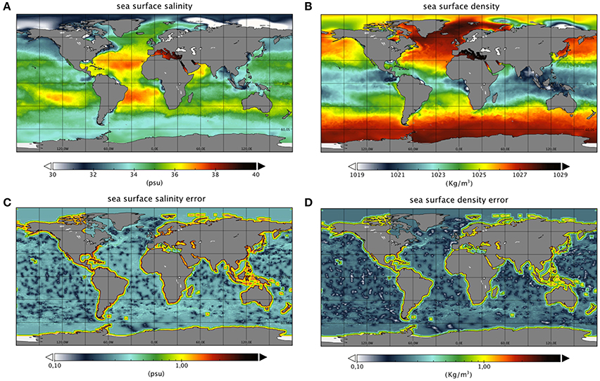
Figure 1. Two examples of SSS (A) and SSD (B) global fields refers to 12 April 2006. The (C,D) show the error related to the SSS and SSD filed respectively (see section A Posteriori Error Estimation).

The method was applied to produce daily (but weekly sampled) global L4 SSS and SSD fields at 1/4° resolution over the period 1993–2016. This dataset is referenced to as SSS_SSD_GLOB_L4_REP in CMEMS catalog.

Four different configurations have been considered in the algorithm calibration phase, given by the choice between two methods and two input sets: Method 1 interpolates SSS, and computes the corresponding SSD through the standard UNESCO (United Nations Educational, Scientific and Cultural Organization) equation of state, combining the interpolated salinity and temperature; Method 2 first interpolates in situ density, and provides a dynamically consistent SSS field by inverting the equation of state to get salinity from density and temperature; Version 1 (V1) data are then obtained using only the real in situ observation in input; Version 2 (V2), includes also pseudo-observations obtained sub-sampling the first guess field.

The Assumptions and Limits of Applicability of the Multidimensional Covariance Model

The fundamental assumptions in OI are that the statistics of the subject data field are stationary (unchanging over the sample period of each map), homogeneous (the same characteristic over the entire data field) and known a priori. Moreover, standard models often make additional assumptions, to simplify the analysis, on covariance isotropy (the same structure in all directions; Thomson and Emery, 2014). Basically, classical space or space-time SSS/SSD true covariances are, in general, spatially anisotropic and non-stationary. In fact, SSS/SSD are sensibly modified across fronts and in mesoscale features, and resulting covariance scales, in turn, change significantly between the cross-front and along-front directions. These structures are also subject to intense temporal variability. On the other hand, in a specific water mass, SSS and SSD are basically modified by isopycnal mixing alone once the effects of large scale freshwater/heat fluxes are filtered out: thus occurring at larger space/time decorrelation scales.

The important problem of the non-stationarity and anisotropy of the true covariance can be partially recovered by representing it as a function of space, time, and (high-pass filtered) SST separation. In fact, in this way the multidimensional covariance automatically adapts to the mesoscale field evolution/frontal displacements. Based on the assumption that different water masses are characterized by different SST/SSS (and generally SSD) values, in open ocean, where surface exchanges mostly occur at the atmospheric scales, a reasonable hypothesis is that, SSS/SSD variations at small scales are correlated to SST variations, filtering out the effects of large scale freshwater/heat fluxes. By contrast, SST and SSS/SSD variations are not necessarily well correlated near the coast, where air–sea interactions and terrestrial freshwater fluxes can result into localized input.

We made here additional assumptions, not only that residual high-pass filtered SSS/SSD variations are due exclusively to advection and mixing, but also that SST, SSS, and SSD mixing are driven by the same dynamics (which is a reasonable assumption in the upper layers, where mixing is mostly driven by turbulent fluxes).

In conclusion, it is possible to see that in case of the water masses have the same temperature but different salinities/densities, the interpolation method will reduce to a standard space-time algorithm (simply because no local SST anomalies are present).

Algorithm and Product Validation

The validation of the modified algorithm (described in section Data and Methods) and of the new SSS/SSD L4 product includes both holdout cross-validation (specifically used to validate the methodology), and comparison with independent in situ measurements. Additionally, the new dataset was validated in terms of effective resolution by computing spatial wavenumber spectra over selected sub-domains and along a repeated TSG transect.

Holdout Validation

As a first step, we validated the methodology using the holdout approach, which is the simplest kind of cross-validation (Hastie et al., 2009). This method splits the dataset into two subsets; an input set and a second one, called holdout set. The latter is used as a fully independent validation dataset. Here, in particular, for each interpolation day, the in situ observations relative to the same day have been taken out and collected to form the holdout set, while all the remaining observations were ingested in the processing. The differences between the L4 data obtained from the input set and the corresponding values in the holdout set are then used for the assessment. The following Tables 1, 2 show the statistics (Mean Bias Error, MBE; Standard Deviation Error, STDE and Root Mean Square Error, RMSE) for the Global L4 dataset of SSS and SSD reprocessed for the whole year 2012 using the “holdout” approach. The Tables 1, 2 highlight that the Version 2 yields lower RMSE values (~ 0.29 psu for the SSS and ~0.26 kg/m³ for the SSD) compared to the Version 1 (~ 0.33 psu for the SSS and ~0.28 kg/m³ for the SSD), reaching the same values found for the first guess (FG). Indeed, because the data in the holdout set were not used in the Multidimensional OI, but they were included in the first guess field computation, this validation is automatically penalizing the former with respect to the latter.

TABLE 1

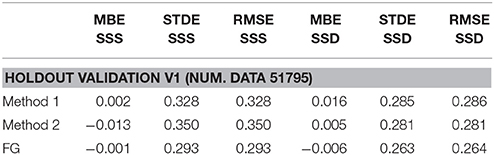
Table 1. Statistics associated with holdout validation for the Version 1(V1) dataset (year 2012).

TABLE 2

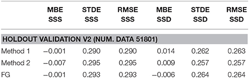
Table 2. Statistics associated with holdout validation for the Version 2 (V2) dataset (year 2012).

Independent in Situ Observation Matchups

The matchup database used for the overall SSS/SSD L4 data independent validation was built by selecting all TSG measurements collected within ±12 h with respect to the nominal interpolation date and co-locating them with the nearest grid point, over the period 1993–2015. The RMSE were computed either by considering all TSG data, or limiting to offshore data (200 km far from the coast), that are not affected by the strong salinity variance observed in the coastal areas close to the main river outflows (Droghei et al., 2016).

The figures below (Figure 2) show the matchup positions between the Global L4 dataset of SSS and TSG measurements and the differences between the interpolated salinity and the relative TSG value. These figures are relative to four different periods displaying homogeneous ship data coverage. Specifically, from 1993 to 2001 only the Gulf Stream and the Labrador Sea are covered, whereas in 2002 the ships' routes covered the entire Atlantic Ocean. The largest coverage has been reached during the period from 2003 to 2014. Finally, the last year of the period, 2015, shows a low number of matchups available, over very sparse trajectories, possibly due to more recent data processing delays. In general, the matchups far from the coast show lower differences between the interpolated data and the TSG salinity (around 0.2 psu), whereas the near coast differences reach higher negative values and their pattern is very noisy. The analysis of Figure 2C, where a more homogenous coverage of TGS data is present, reveals that the differences remain generally below ±0.2 psu in all offshore regions of the global oceans with the exception of Caribbean seas (30 N 50 W) where differences of the order of 1 psu are found and Gulf stream region, where a negative bias of approximately 0.5 psu is obtained.

FIGURE 2

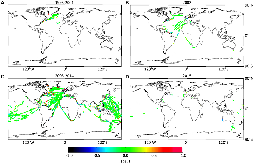
Figure 2. Matchup positions between Global L4 dataset of SSS and TSG measurements. The four pictures show four different periods where the TSG coverage was more homogeneous. (A) 1993-2001; (B) 2002; (C) 2003-2014; (D) 2015. The color of the dots, furthermore, provides the differences between the interpolated salinity and the relative TSG value (in psu).

In Situ Matchup Global Statistics

The RMSE computed from SSS/SSD L4 data (SSS_SSD_GLOB_L4_REP) is generally lower than or comparable to the reference products: version 3 of ARMOR3D (in this case we have an improvement in RMSE of about 30%, see Table 3) dataset and CORA (our first guess, see section Data and Methods), with a few exceptions at the beginning of the time series. The number of matchup data, however, increases significantly with time, and only after 2003 a more homogeneous coverage is provided by TSG, even if matchups remain mostly confined to the mid-low latitudes, and prevalently located in the Northern Hemisphere, more than 1.5 million, representing approximately the 28% of the total number of TSG data. A significant portion of the TSG data are found in coastal areas, almost a million, that are characterized by high salinity variability (partly related to freshwater discharge by major rivers), which leads to an overall RMSE of 0.84 (Figure 3A). The differences are significantly reduced and more stable in time when considering only the offshore TSG data, with an overall RMSE of 0.25 psu (Figure 3B).

TABLE 3

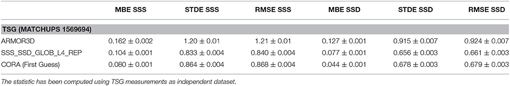
Table 3. Statistic's comparison among ARMOR3D, SSS_SSD_GLOB_L4_REP and first guess datasets for the period 1993–2015.

FIGURE 3

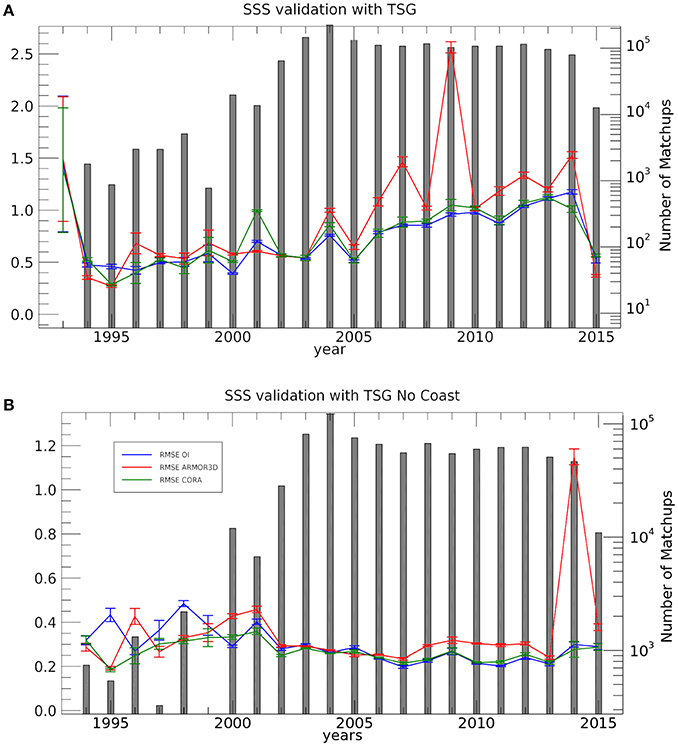
Figure 3. Sea Surface Salinity time series of RMSE (and the corresponding error bars) between TSG observations and SSS_SSD_GLOB_L4_REP (blue), ARMOR3D (red), CORA (green). The number of co-located observations available each year is indicated, in logarithmic scale, by gray bars. The statistics were obtained using (A) all TSG data available (including coastal areas), (B) limiting to TSG data collected offshore (>200 km).

The same behaviors are found in the statistics computed from SSD data. An overall RMSE of 0.68 kg/m3 is found considering all TSG data (Figure 4A), but the differences are significantly reduced, and stable in time, when considering only the offshore TSG data, with an overall RMSE of 0.21 kg/m³ (Figure 4B). For all calculations, we also estimated the significance of the statistics, namely by calculating 95% confidence intervals through a Monte Carlo approach: doubling the standard deviation of the statistics carried out from 2000 resamples with replacement (Efron and Tibshirani, 1993). The following Tables 3, 4 report the validation statistics for our SSS/SSD L4 product (SSS_SSD_GLOB_L4_REP), previous surface ARMOR3D fields and CORA first Guess for the entire period 1993–2015, showing the effective reduction, of about 30%, of the SSS/SSD L4 data RSME in respect to the previous version of ARMOR3D. It must be kept in mind, anyway, that the comparison between point-wise in situ measurements and mapped products based on satellite observations is affected also by representativeness issues. In practice, in situ measurements are typically obtained at a given depth below the surface and are representative of a very localized water mass, while the satellite is clearly providing an average signal emerging from a large footprint. To really assess the mutual error between different sources defined at different scales at least three independent sources of co-located observations would be need. In that case, absolute errors associated with the single instrument/product could be estimated through the Triple Collocation (TC) method (e.g. Stark et al., 2008). Unfortunately, then, we do not have enough data to follow this approach here.

FIGURE 4

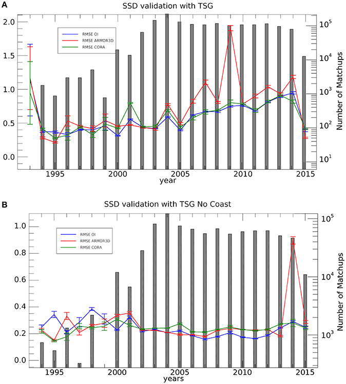
Figure 4. Sea Surface Density time series of RMSE (and the corresponding error bars) between TSG observations and SSS_SSD_GLOB_L4_REP (blue), ARMOR3D (red), CORA (green). The number of co-located observations available each year is indicated, in logarithmic scale, by gray bars. The statistics were obtained using (A) all TSG data available (including coastal areas), (B) limiting to TSG data collected offshore (>200 km).

TABLE 4

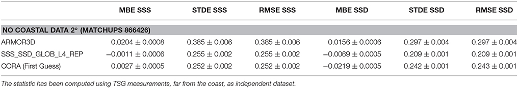
Table 4. Statistic's comparison among ARMOR3D, SSS_SSD_GLOB_L4_REP and first Guess datasets for the period 1993–2015, considering no coastal data (with a 2° distance from the coast).

Power Spectral Density

Looking at spatial wavenumber spectra, it is possible to show that the multidimensional OI method significantly increases the L4 effective resolution with respect to standard products. This has been done here in two different steps.

First, spatial wavenumber spectra (Power Spectral Densities, PSD) have been estimated and compared here only between interpolated SSS/SSD datasets, concentrating on four land free portions of the domain and considering a temporal average over the entire 2010 (see Figure 5). Successively, a specific analysis has been carried out on the smaller scales, by comparing the PSD obtained from both in situ and interpolated observations along one repeated TSG track.

FIGURE 5

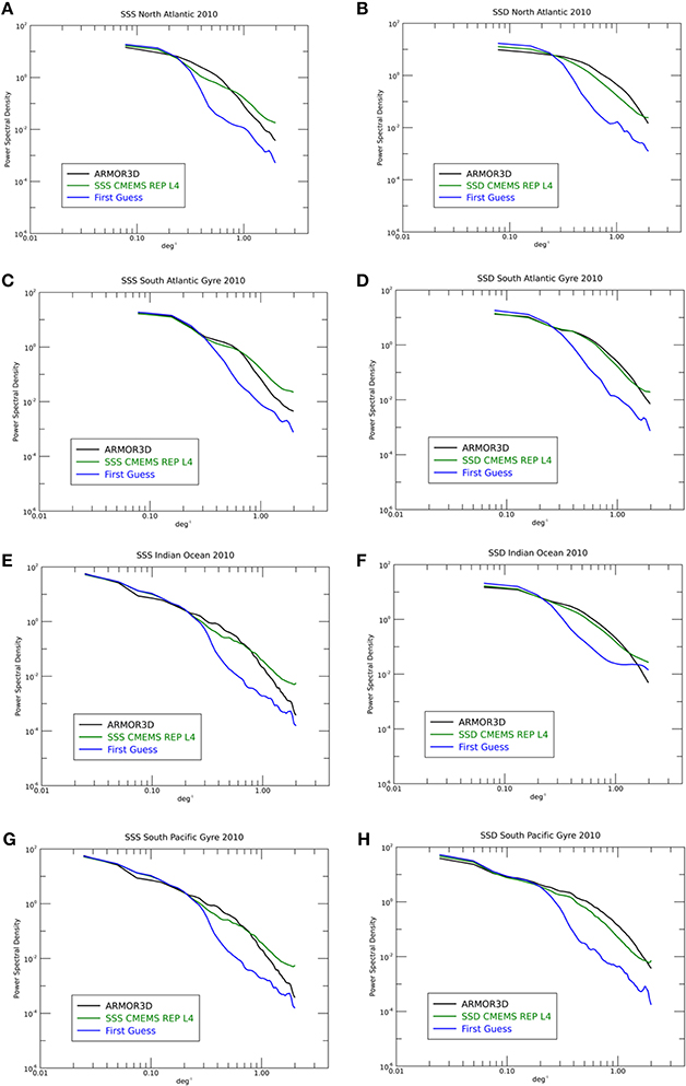
Figure 5. Comparison among: previous version of surface ARMOR3D, CMEMS REP L4 and first guess tracer power spectral density estimated only on four land free portions of the domain: SSS (left panel), SSD (right panel). Considering as sample the average over the entire 2010. The figures (A,C,E,G) show SSS Power spectral densities plots for the North Atlantic, the South Atlantic Gyre, the Indian Ocean and the South Pacific Gyre basins, respectively. The figures (B,D,F,H) show SSD Power spectral densities plots for the North Atlantic, the South Atlantic Gyre, the Indian Ocean and the South Pacific Gyre basins, respectively.

In the first case, PSD were computed taking latitudinal variations only (we take latitudinal variations and not longitudinal because they represent the same physical distance), and averaging the results obtained at each longitude and each time to obtain a single spectrum. A total of 52 snapshots have been considered, the time difference between two snapshots is 1 week. To reduce spectral leaking, a Blackman-Harris windowing function has been applied before computing the Fast Fourier Transform. Four different subdomains have been considered as detailed in Table 5.

TABLE 5

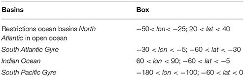
Table 5. Geographical limits of the subdomains considered for the spectral analysis.

As expected, CORA SSS-PSD (first guess) shows an abrupt variance drop already at low wavenumber (< 0.2 deg⁻¹). The SSS spectrum computed from the version 3 of ARMOR3D also shows a steep variance reduction (with slope exceeding k⁻³) at approximately 0.4 deg⁻¹. Conversely, the new CMEMS SSS L4 spectra show the highest variance even at low wavenumbers (and a spectral slope comprised between k⁻³ and k^−5/3), with an effective resolution of about twice/four time the grid nominal resolution, namely between 1/2° and 1°, where the noise finally flattens the spectrum (see also Droghei et al., 2016). The spectral behaviors are consistent among all sub domains. The SSD PSDs show similar behaviors as SSS PSDs, the first guess field always displaying a substantial variance drop at wave number greater than 0.2 deg⁻¹ with both ARMOR3D (version 3) and new CMEMS SSD showing very similar values up to approximately 0.8 deg⁻¹ where ARMOR3D spectral slope get significantly steeper, missing information, and also in these cases all subdomains display consistent feature among the different datasets.

To verify that the higher variance found at the large mesoscale range is not given by noise or artifacts, we also compared co-located SSS TSG and SSS products spectra from repeated high-resolution TSG measurements collected along a merchant shipping route, which provides enough data to minimize the error in spectral computation. To this aim, we started from same data used by Kolodziejczyk et al. (2015), i.e., observations from Toucan and Colibri ships (their Table 1), which span over almost 10 years and cover a transect in the North Atlantic, looking specifically at data collected between 24°N and 34°N. These data include the region of the Azores Current/Front, which is known to be very active at the mesoscale (and sub-mesoscale) (e.g., Kolodziejczyk et al., 2015, and references therein). To compute the PSD, we sub-divided the TSG tracks in 600 km-long complete transects, which correspond approximately to 1 day of data. For each transect, the closest SSS L4 data have been selected (both in space and in time), and match-up and TSG data were then interpolated on a 1 km regular grid to compute the PSD. All spectra have been finally truncated at the Nyquist frequency of the original dataset. As a consequence, even if the direct comparison will be likely affected by synopticity issues, as our analyses are provided only at weekly sampling, the spectra are expected to provide a consistent comparison. The PSD estimated from TSG, CMEMS SSS L4 and from our first guess (CORA) are shown in Figure 6. They show that a significant amount of variance is actually recovered through the multivariate interpolation.

FIGURE 6

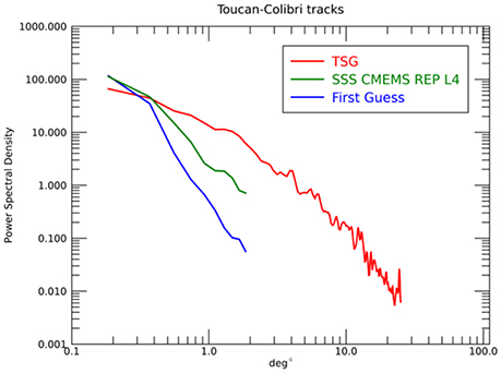
Figure 6. Mean PSD computed from CMEMS REP L4 SSS, CORA SSS, and TSG observations along the Toucan and Colibri ships' routes between 2003 and 2011, in the sector comprised between 24°N and 34°N.

To demonstrate that the signals retrieved do not originate from noise, three examples of observed transects are displayed in Figure 7. They compare data collected within a temporal window of less than 2 days (but always greater than 1 day), and show that the CMEMS REP L4 is able to reproduce at least the main deviations from the mean gradient field found in the CORA field. Consistently with the estimated PSD, the amplitude of the retrieved anomalies is clearly much smaller than those found in TSG data, but still represents a significant improvement with respect to standard products. The three signals have been detrended so that their PSD amplitude at 0 freq. should coincide at zero frequency. Relative excess amplitude at 0.2 deg⁻¹ then comes out directly from PSD computation.

FIGURE 7

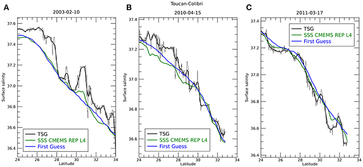
Figure 7. Comparison between TSG (black/gray), CMEMS REP L4 and CORA (first guess) SSS along the Toucan and Colibri ships' routes on three selected dates: (A) 2003-02-01; (B) 2010-04-15; (C) 2011-03-17. The black line shows TSG data smoothed through a ¼° moving average while original data are shown in light gray.

A Posteriori Error Estimation

OI formal error basically measures the amount of information that effectively enters the analysis, and should not be considered as a measure of the “true” error. In fact, if compared to differences with independent observations, they are expected to reflect the limits of the assumptions made in the error covariance estimation. It should indeed be considered as a conservative estimate of effective errors (see Equation 2), and in our case it clearly demonstrates the positive impact of Argo measurements starting from year 2002 (Figure 8).

FIGURE 8

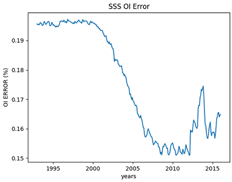
Figure 8. Monthly temporal series from 1993 to 2016 of the spatial averaged OI formal error.

On the other hand, the formal error can also be used to tune a posteriori the error estimate to be associated with the retrieved fields, by directly comparing formal errors and observed differences from matchup data. Figure 9 thus shows the RMS and mean bias of the differences between the REP L4 SSS and TSG SSS as a function of the formal interpolation error expressed in percentage (binned at 10% intervals). In this case, scatter plots were displayed separately for purely offshore data and purely coastal data (within 200 km from land), respectively, as they are expected to show very different performances. Indeed, the RMSE values corresponding to the coastal data are higher, almost doubled, than the RMSE for offshore data, but in both cases a linear relation can be hypothesized (at least up to 60%, while not enough matchup can be associated with higher values). Density plots of the absolute value of differences between Global REP L4 SSS and TSG LEGOS as a function of the interpolation error are also presented see Figure 10. A linear regression fit has then been computed for both coastal and offshore data from Figure 9, and corresponding coefficients will be used to convert the interpolation error from percentage to psu values in the V4 release of CMEMS product (as in Figures 2C,D).

FIGURE 9

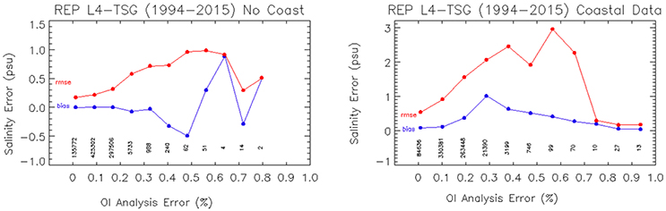
Figure 9. RMSE (red line) and mean bias (blue line) of the differences between Global REP L4 SSS data and SSS from TSG LEGOS as function of the interpolation error. The plot on the left shows the statistics only for the no coast data (2° far from the coast). The plot on the right show statistics for the coastal data. The number of matchups used to carry out the statistic are showed below the lines.

FIGURE 10

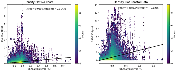
Figure 10. Density plots of the absolute value of differences between Global REP L4 SSS and TSG LEGOS as a function of the interpolation error. The black lines are the linear fit computed with slope and intercept showed in the upper part of the figures. The color bars show the number of counts (in logarithmic scale). Left image shows no coast differences (2° far from the coast) and the right image shows only coastal differences.

Conclusions

In this work, the multi-dimensional OI method originally proposed by Buongiorno Nardelli (2012) has been modified and adapted to produce a long time series of Global SSS/SSD fields, with a nominal spatial resolution of ¼°, daily (with weekly sampling), covering the entire period 1993–2016. The dataset, presently distributed through CMEMS as part of GLOBAL_REP_PHY_001_021 product (as dataset SSS_SSD_GLOB_L4_REP), combines high-resolution SST satellite measurements with in situ salinity and density measurements in order to get a more accurate description of both parameters at the sea surface, even during periods characterized by extremely sparse in situ data coverage. In the new scheme, pseudo-observations obtained subsampling the first guess field have been added as input to the interpolation to reduce the biases due to the combination of data sparseness and large SSS variability in coastal areas, and to avoid spurious signals potentially appearing in case of prolonged data voids. The validation of the new scheme was first carried out using the holdout approach, evidencing a significant improvement with respect to the original configuration (with a ~10% reduction of the RMSE). Successively, a fully-independent validation of the entire re-processed dataset with TSG observations was performed, displaying significant improvements both in terms of statistics of the differences between interpolated data and in situ observations, and in terms of spatial scales that are effectively resolved by the multivariate combination with high resolution SST data. In addition, the increase in the effective resolution of the multidimensional L4 dataset with respect to standard products has been analyzed by looking at spatial wavenumber spectra. Firstly, SSS/SSD Power Spectral Densities were estimated and compared concentrating on four land free portions of the domain and considering a temporal average over the entire 2010. Secondly, co-located SSS TSG and SSS L4 products were used to compute wavenumber spectra from repeated high-resolution TSG measurements, verifying that the higher variance found at the large mesoscale range is not given by noise or artifacts, but rather reflects the ability to reconstruct at least part of the observed mesoscale field. Corresponding increase of retrieved spatial variance with respect to standard univariate products attains around a factor 10 at 1/2° wavelengths, though remaining below that estimated from TSG data by approximately the same factor.

Indeed, this new time series will allow to carry out analyses of salinity and density variability at different scales, as it provides information up to the large mesoscale, but also over temporal scales of interest for the assessment of interannual changes. On the other hand, a cautionary approach must be followed when analyzing changes over longer periods (i.e., decadal trends), as both the number of input observations and independent validation data is considerably lower before 2002 (this is particularly evident when looking at OI formal error). Consistently with previous results (Buongiorno Nardelli, 2012; Buongiorno Nardelli et al., 2016; Droghei et al., 2016), however, the analyses presented here confirm that the multivariate OI combining satellite SST and in situ SSS/SSD data represents a powerful approach to provide a better characterization of the ocean surface salinity and density variability, despite the fact that the product quality degrades near the coasts. Indeed, improvements can be found only where SSS and SST small scale anomalies are correlated, while the technique basically reduces to a standard space-time salinity/density interpolation in areas characterized by uniform SST patterns and thermohaline compensation, respectively.

Author Contributions

All authors listed have made a substantial, direct and intellectual contribution to the work, and approved it for publication.

Conflict of Interest Statement

The authors declare that the research was conducted in the absence of any commercial or financial relationships that could be construed as a potential conflict of interest.

Acknowledgments

This work was carried out within the Multi Observations Component of the GLOBAL CMEMS Monitoring and Forecasting Centre, founded by a subcontracting agreement between the Italian National Research Council (CNR) and Collecte Localisation Satellites (CLS). The study has been conducted using products disseminated through the European Copernicus Marine Service, the Global Ocean Surface Underway Data project, Sea surface salinity data made freely available by the French Sea Surface Salinity Observation Service (http://www.legos.obs-mip.fr/observations/sss/), and the Global High Resolution Sea Surface Temperature project. We thank A. Pisano for his help and feedbacks.

References

Alory, G., Delcroix, T., Téchiné, P., Diverrès, D., Varillon, D., Cravatte, S., et al. (2015). The French contribution to the voluntary observing ships network of sea surface salinity. Deep Sea Res. 105, 1–18. doi: 10.1016/j.dsr.2015.08.005

CrossRef Full Text | Google Scholar

Balmaseda, M. A., Hernandez, F., Storto, A., Palmer, M. D., Alves, O., Shi, L., et al. (2015). The ocean reanalyses intercomparison project (ORA-IP). J. Operat. Oceanogr. 8, S80–S97. doi: 10.1080/1755876X.2015.1022329

CrossRef Full Text | Google Scholar

Buongiorno Nardelli, B. (2012). A novel approach for the high-resolution interpolation of in situ sea surface salinity. J. Atmos. Ocean. Technol. 29, 867–879. doi: 10.1175/JTECH-D-11-00099.1

CrossRef Full Text | Google Scholar

Buongiorno Nardelli, B., Droghei, R., and Santoleri, R. (2016). Multi-dimensional interpolation of SMOS sea surface salinity with surface temperature and in situ salinity data. Remote Sens. Environ. 180, 392–402. doi: 10.1016/j.rse.2015.12.052

CrossRef Full Text | Google Scholar

Cabanes, C., Grouazel, A., Schuckmann, K. V., Hamon, M., Turpin, V., Coatanoan, C., et al. (2013). The CORA dataset: validation and diagnostics of in-situ ocean temperature and salinity measurements. Ocean Sci. 9, 1–18. doi: 10.5194/os-9-1-2013

CrossRef Full Text | Google Scholar

Droghei, R., Nardelli, B. B., and Santoleri, R. (2016). Combining in situ and satellite observations to retrieve salinity and density at the ocean surface. J. Atmos. Ocean. Technol. 33, 1211–1223. doi: 10.1175/JTECH-D-15-0194.1

CrossRef Full Text | Google Scholar

Efron, B., and Tibshirani, R. J. (1993). An Introduction to the Bootstrap. Chapman & Hall/CRC, 45–59.

Frankignoul, C., Deshayes, J., and Curry, R. (2009). The role of salinity in the decadal variability of the North Atlantic meridional overturning circulation. Clim. Dynam. 6, 777–793. doi: 10.1007/s00382-008-0523-2

CrossRef Full Text | Google Scholar

Gaillard, F., Autret, E., Thierry, V., and Galaup, P. (2009a). Quality control of large Argo datasets. J. Atmos. Ocean. Technol. 26, 337–351. doi: 10.1175/2008JTECHO552.1

CrossRef Full Text | Google Scholar

Gaillard, F., Brion, E., and Charraudeau, R. (2009b). ISAS–V5: Description of the Method and User Manual. IFREMER Rapport LPO, 9–04.

Gaillard, F., Reynaud, T., Thierry, V., Kolodziejczyk, N., and Von Schuckmann, K. (2016). In situ–based reanalysis of the global ocean temperature and salinity with ISAS: variability of the heat content and steric height. J. Clim. 29, 1305–1323. doi: 10.1175/JCLI-D-15-0028.1

CrossRef Full Text | Google Scholar

Good, S. A., Martin, M. J., and Rayner, N. A. (2014). EN4: quality controlled ocean temperature and salinity profiles and monthly objective analyses with uncertainty estimates. J. Geophys. Res. 118, 6704–6716. doi: 10.1002/2013JC009067

CrossRef Full Text | Google Scholar

Guinehut, S., Dhomps, A. L., Larnicol, G., and Le Traon, P. Y. (2012). High resolution 3-D temperature and salinity fields derived from in situ and satellite observations. Ocean Sci. 8, 845–857. doi: 10.5194/os-8-845-2012

CrossRef Full Text | Google Scholar

Hastie, T., Tibshirani, R., and Friedman, J. (2009). “Unsupervised Learning.” The Elements of Statistical Learning. New York, NY: Springer.

Google Scholar

Held, I. M., and Soden, B. J. (2006). Robust responses of the hydrological cycle to global warming. J. Climate 19, 5686–5699. doi: 10.1175/JCLI3990.1

CrossRef Full Text | Google Scholar

Kolodziejczyk, N., Hernandez, O., Boutin, J., and Reverdin, G. (2015). SMOS salinity in the subtropical North Atlantic salinity maximum: 2. Two-dimensional horizontal thermohaline variability. J. Geophys.Res. Oceans, 120, 972–987. doi: 10.1002/2013JC009610

CrossRef Full Text | Google Scholar

Reynolds, R. W., Smith, T. M., Liu, C., Chelton, D. B., Casey, K. S., and Schlax, M. G. (2007). Daily high-resolution-blended analyses for sea surface temperature. J. Clim. 20, 5473–5496. doi: 10.1175/2007JCLI1824.1

CrossRef Full Text | Google Scholar

Schmitt, R. W., Boyer, T., Lagerloef, G., Schanze, J., Wijffels, S., and Yu, L. (2008). Salinity and the global water cycle. Oceanography 21, 12–19. doi: 10.5670/oceanog.2008.63

CrossRef Full Text | Google Scholar

Stark, J. D., Donlon, C., O'Carroll, A., and Corlett, G. (2008). Determination of AATSR biases using the OSTIA SST analysis system and a matchup database. J. Atmos. Ocean. Technol. 25, 1208–1217. doi: 10.1175/2008JTECHO560.1

CrossRef Full Text | Google Scholar

Thomson, R. E., and Emery, W. J. (2014). Data Analysis Methods in Physical Oceanography. Newnes.

Trenberth, K. E., Smith, L., Qian, T., Dai, A., and Fasullo, J. (2007). Estimates of the global water budget and its annual cycle using observational and model data. J. Hydrometeorol. 8, 758–769. doi: 10.1175/JHM600.1

CrossRef Full Text | Google Scholar

Umbert, M., Hoareau, N., Turiel, A., and Ballabrera-Poy, J. (2014). New blending algorithm to synergize ocean variables: the case of SMOS sea surface salinity maps. Remote Sens. Environ. 146, 172–187. doi: 10.1016/j.rse.2013.09.018

CrossRef Full Text | Google Scholar