Local Biomass Baselines and the Recovery Potential for Hawaiian Coral Reef Fish Communities

Introduction

The fragility of coral reefs combined with the pervasiveness of human impacts threatens the long-term future of these ecosystems (Mora et al., 2016; Hughes et al., 2017). The continuing degradation of coral reefs in the Anthropocene era has hastened calls for scientists to provide information that enables environmental decision-making and effective prioritization of management efforts (McNie, 2007; Cvitanovic et al., 2015). One management strategy that could simultaneously address local stressors to coral reefs and increase their resilience to global climate threats is marine spatial planning (MSP) (Pandolfi et al., 2011)—the systematic organization and zoning of human use of the marine environment into designated areas (Gilliland and Laffoley, 2008). Scientists can assist MSP efforts by providing spatially-explicit, locally-relevant benchmarks essential to the process (Day, 2008). This requires an understanding of how habitat and oceanographic conditions influence coral reef ecosystem state, as well as how those states have been influenced by human impacts (Crowder and Norse, 2008).

Multiple biotic (e.g., coral and algal cover) and abiotic (e.g., substrate complexity) factors contribute to the considerable natural variability among coral reef ecosystems. When considering the fish assemblages of these systems, habitat characteristics such as coral cover and substrate complexity greatly influence potential species richness and diversity (Chabanet et al., 1997). At larger scales, coral reef fish communities are also influenced by oceanographic factors such as oceanic productivity, temperature, and wave energy (Friedlander et al., 2003; Heenan and Williams, 2013; Williams et al., 2015). Furthermore, characteristics that relate to fishing pressure, such as distance to human population centers, have been shown to influence fish biomass at multiple scales (Brewer et al., 2009). Most coral reefs are subject to human impacts, but these impacts operate on top of background variation in environmental conditions (Williams et al., 2015). Given the range of ecosystem status and trends, there are a variety of options for managers to consider in addressing potential and on-going stressors. By integrating multiple management objectives and benchmarks, MSP has the potential to effectively account for both the natural and anthropogenic heterogeneity that exists across different stretches of coasts and seascapes (Crowder and Norse, 2008).

Baselines, such as pristine reef fish biomass, can be one such benchmark for guiding MSP efforts. Estimates of baseline reef fish biomass (Nadon et al., 2012; MacNeil et al., 2015; Williams et al., 2015) provide a means for quantifying the extent and spatial variation of depletion (i.e., difference between baseline and present-day state). Areas that have a high baseline biomass (i.e., have a high natural capacity to support fish biomass) and whose present-day levels of fish biomass already closely matches their baseline could be highly valued, and thus prioritized for conservation purposes. On the other hand, were conservation planners and managers more concerned with restoring areas in most urgent need of attention, it would be useful to identify those areas that have experienced the most amount of depletion (i.e., have the greatest potential for recovery). Ultimately management objectives and the decision to protect the strong or the weak (Game et al., 2008) is a societal choice but here we present both baseline biomass and recovery potential (i.e., the difference between present-day and baseline biomass), as a useful framing to guide such decisions.

Knowing the baseline state of an ecosystem with certainty requires a time series of data, dating from prior to the onset of degradation. However, sufficiently long-term trends are exceedingly rare for coral reef ecosystems. Alternatively, this can be done spatio-temporally (e.g., using a chronosequence) whereby time since protection for different areas can be used to generate expectations about recovery (McClanahan et al., 2007, 2016; MacNeil et al., 2015). Finally, in the absence of such a chronosequence, baseline fish biomass can be estimated spatially, for example, by comparing (Friedlander and DeMartini, 2002) or modeling (Williams et al., 2015; D'agata et al., 2016) reefs along a gradient of human-induced impact. Here, we apply this spatial approach to estimating both baseline biomass and the recovery potential of coral reef fish assemblages around the main Hawaiian Islands.

This study is timely because, following unprecedented levels of coral bleaching and mortality observed throughout Hawaii between 2015 and 2016, Hawaii's Division of Aquatic Resources (DAR) became interested in developing management strategies to promote recovery of its coral reef communities, as well as resilience to likely future events (University of Hawaii Social Science Research Institute, 2017). Their systematic review of the literature and synthesis of expert opinion highlighted two proposed actions that addressed the management goal of promoting coral recovery (University of Hawaii Social Science Research Institute, 2017): (i) the establishment of a network of permanent no-take marine protected areas (MPAs) and (ii) the establishment of a network of herbivore management areas. MPAs are a widely-used conservation tool that function by protecting the diversity, density, and size of targeted species found within the reserve. By preserving ecosystem function, it is believed that MPAs create stability in community assemblages and increase resilience to future disturbance events (Mellin et al., 2016). Herbivorous fishes, in particular, are believed to play a disproportionately large role in ecosystem processes of coral reefs, with different herbivorous functional groups mediating different ecological processes. For example, by keeping algal communities in a cropped and productive state, browsers have been implicated in preventing the establishment of macroalgae, while grazers, scrapers, and excavators may facilitate the settlement, survival and growth of crustose coralline algae and coral (Hatcher and Larkum, 1983; Hay et al., 1983; Steneck, 1988; Bellwood and Choat, 1990; Green and Bellwood, 2009). Overall, by managing coral-algal dynamics, herbivores can enhance coral reef resilience to bleaching events by preventing algal overgrowth (Graham et al., 2015). Given the interest from local managers in the potential for both no-take MPAs (i.e., protection of all reef fishes) and herbivore management areas (i.e., protection of just herbivorous fishes) in coral reef resiliency planning (University of Hawaii Social Science Research Institute, 2017), here we focus on both total reef fish community biomass, as well as the herbivorous fish component of the assemblage.

Specifically, we use a large-scale dataset [NOAA's Pacific Reef Assessment and Monitoring Program (Pacific RAMP, Coral Reef Ecosystem Program: Pacific Islands Fisheries Science Center, 2007)] to characterize coral reef fish assemblages throughout the main Hawaiian Islands. We implement a Bayesian, hierarchical framework to: (i) account for the hierarchical nature of processes affecting coral reefs (MacNeil et al., 2009) as well as the hierarchical design of Pacific RAMP (i.e., sites nested within sectors nested within islands nested within region); (ii) model spatially nested effects such that broad-scale processes are allowed to vary among locations, allowing for prediction at local scales relevant to management; and (iii) quantify uncertainty in our estimation of both baseline biomass and recovery potential (Ellison, 1996). We do this by first modeling herbivore and total reef fish biomass as response variables to multiple habitat, oceanographic, and human drivers. Then, by setting human population density to the minimum level found in our dataset, (i.e., minimizing the effect of humans on fish biomass), we estimate: (i) baseline biomass and (ii) percent recovery potential or the proportional increase from present-day to baseline biomass across the main Hawaiian Islands, while incorporating the uncertainty associated with the effect of humans.

Methods

Data Collection

Fish surveys were conducted throughout the main Hawaiian Islands in 2012, 2013, and 2015 (Coral Reef Ecosystem Program: Pacific Islands Fisheries Science Center, 2007) using a stratified random design sampling 25 sub-island sectors (Figure 1; Maui-Hana was not analyzed because only one site was available here, and no data was available for Maui-Southeast). Refer to Heenan et al. (2017) for a more in-depth description of our data, including how the survey method used by this monitoring program compares with the more commonly used belt transect method for surveying fish. These 3 years of data were selected to represent a recent snapshot, i.e., what we refer to as “present-day” biomass in our analysis. Sector divisions were based on broad-scale categorizations (i.e., presumed fishing pressure, including shoreline accessibility, and coarse habitat type), and are currently being used as part of the survey design for NOAA's Pacific RAMP.

FIGURE 1

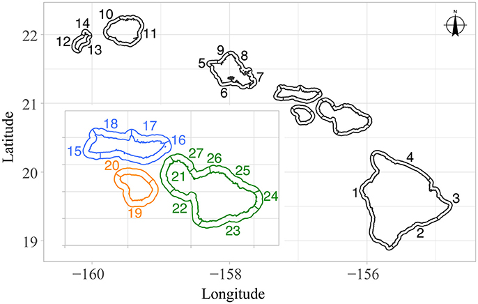
Figure 1. Sub-island sectors of the main Hawaiian Islands, used in the NOAA Pacific Reef Assessment and Monitoring Program's survey design, as well as in our hierarchical analysis. Sector names, as they appear in the text, include: 1, Hawaii-Kona; 2, Hawaii-Southeast; 3, Hawaii-Puna; 4, Hawaii-Hamakua; 5, Oahu-Kaena; 6, Oahu-South; 7, Oahu-East; 8, Oahu-Northeast; 9, Oahu-Northwest; 10, Kauai-Na Pali; 11, Kauai-East; 12, Niihau-West; 13, Niihau-East; 14, Niihau-Lehua; 15, Molokai-West; 16, Molokai-South; 17, Molokai-Pali; 18, Molokai-Northwest; 19, Lanai-South; 20, Lanai-North; 21, Maui-Lahaina; 22, Maui-Kihei; 23, Maui-Southeast; 24, Maui-Hana; 25, Maui-Northeast; 26, Maui-Kahului; 27, Maui-Northwest. Note that sector widths are not to scale (i.e., the sampling domain for fish surveys only extends from the shoreline to 30 m depth).

Each survey consisted of a pair of divers, simultaneously collecting data for adjacent survey areas (7.5 m radius cylinders) (Ayotte et al., 2011). Diver comparisons are published annually in our monitoring reports as quality control measures that assess whether any large diver-associated bias exists with regards to either the total biomass and/or species diversity being recorded; none were found in the datasets analyzed here (Heenan et al., 2012; McCoy et al., 2015). Site-level total and herbivorous reef fish biomasses (g m⁻²) were calculated by using species-specific length-weight conversion parameters (Froese, and Pauly, 2016) and by averaging the two diver replicates. For our list of herbivore reef fish species, we follow the trophic classifications of Sandin and Williams (2010) (Supplementary Table S1). Finally, roving predators (e.g., sharks, large jacks, rays, barracudas, tunas) were excluded from all biomass calculations, because they are not well sampled by small-scale survey methods and because there is potential for bias due to behavioral differences of those species in relation to divers (i.e., diver-attracted and diver-avoiding behaviors) at different levels of fishing pressure and human presence (Gray et al., 2016). Other targeted species that may exhibit these behaviors are still included in our analysis which would tend to exaggerate differences between heavily-fished and remote locations. For Hawaii, bias from fish behavior appears to be limited to locations with the heaviest fishing pressure (i.e., Oahu). While this effect should certainly be controlled for in certain contexts (e.g., smaller scale, site-level comparisons), observed biomasses at broader scales such as the scale of this study are still large enough to allow for relative comparisons.

Based on the numerous studies that have utilized the Pacific RAMP reef fish dataset, we expect a priori the following broad categories to be important for our model: benthic cover (Williams et al., 2015; Heenan et al., 2016), physical characteristics of the habitat (Williams et al., 2015; Cinner et al., 2016; Heenan et al., 2016; Robinson et al., 2017), oceanographic environment (Williams et al., 2015; Cinner et al., 2016; Heenan et al., 2016; Robinson et al., 2017), and human population density (Williams et al., 2015; Heenan et al., 2016; Robinson et al., 2017). However, the relative strength of these different variables for different locations at a sub-island scale—crucial information for local management decisions—remained unclear. A list of all candidate variables can be found in Table 1.

TABLE 1

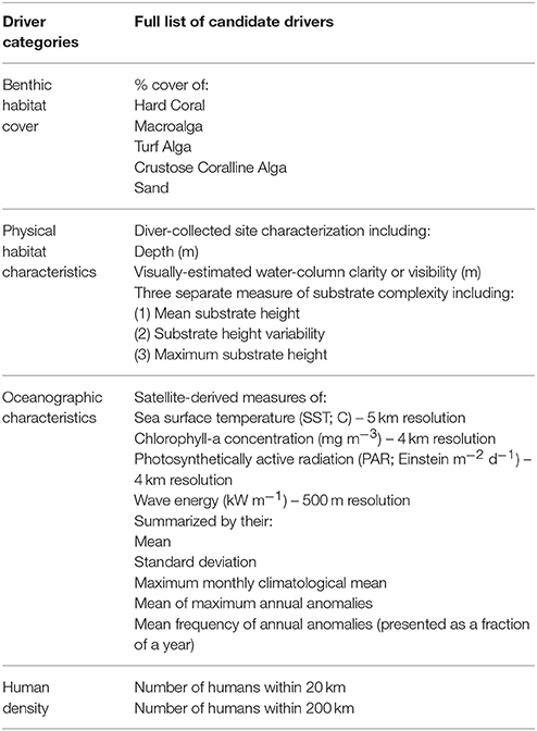
Table 1. List of all candidate drivers for modeling total and herbivorous reef fish in the main Hawaiian Islands.

To estimate benthic cover, a photo quadrat transect (n = 30 photos taken through the middle of the survey area) was taken at each fish survey site. Photos were then processed using point count software (n = 10 points per photo), either CPCe (2012–2014 data) or CoralNet (2015 data). At each site, divers also recorded in situ physical characteristics including depth, water clarity, and substrate complexity. Here, we consider underwater water clarity to be an environmental driver rather than a proxy for detectability—as surveys were not conducted when visibility was low. Divers assessed substrate complexity by estimating the proportion of the survey area that fell into five substrate height categories: 0–25; 25–50; 50–100; 100–150 cm; and >150 cm, later summarized as a weighted mean of each bin's midpoint. Other metrics of substrate complexity included the maximum substrate height and the standard deviation of the difference between each substrate bin and the overall weighted mean (i.e., a measure of substrate height variability).

Biophysical oceanographic variables were derived from remotely-sensed data to provide site-level estimates related to sea surface temperature, chlorophyll-a concentration, photosynthetically active radiation (i.e., irradiance), and wave power. For ocean color metrics (i.e., chlorophyll concentration and photosynthetically active radiation), a “quality control mask” (Gove et al., 2013; Wedding et al., 2017) is applied that removes data pixels known to be optically erroneous due to issues associated with shallow water bottom reflectance. Wave power, which incorporates both wave period and wave height and therefore represents a more realistic estimate of wave-induced stress on coral reefs, was obtained using University of Hawaii's high-resolution SWAN (Simulating WAves Nearshore) wave model (Li et al., 2016). All metrics were based on 2003–2014 time series data (other than wave energy, which was based on data through 2013), summarized by various standard temporal statistics (Table 1), and joined to our fish dataset at the site-level based on averaging the three nearest pixels to each fish survey site. In other words, all oceanographic metrics are summary statistics, for which temporal variation has been compressed.

We use human density as a coarse proxy for human impacts on the fish community including coral reef fishing catch and effort, as well as other human related stressors, such as the indirect effects of land-based sources of pollution. Site-level human-related impact was characterized as the number of people (United States Census Bureau, 2010) within a certain distance of each fish survey site. Two spatial scales were explored for this purpose: number of people within 20 km and within 200 km.

Model Construction

All site-level data and metadata needed for this analysis can be found in Supplementary Text S1A,B. A total of N = 717 fish surveys were used for this analysis (Figure 2; four sites had no herbivores and were not included for the herbivore analysis, as all data were log-transformed; Supplementary Figure S1A). We removed all sites that fell in areas where fishing was restricted or prohibited (Friedlander et al., 2014). We log-transformed our positive fish biomass densities to obtain normally distributed residual errors, and thus model the response as a normal distribution. All logs mentioned herein refer to the natural log. Furthermore, site-level maps of all covariate data were produced in order to verify the appropriate scale(s) at which they should enter the analysis. All (Supplementary Figures S1B–K) exhibited intra-sector variation (e.g., Figure 3 coral cover), indicating that they could potentially be informative at this scale and thus, should enter the analysis at the site-level.

FIGURE 2

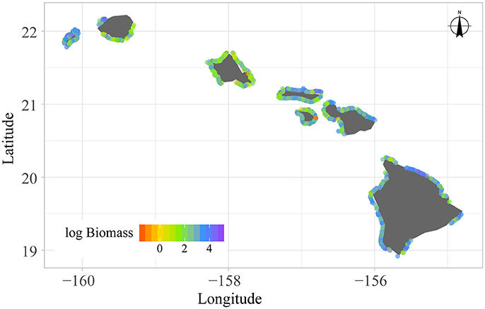
Figure 2. Observed log biomass of total reef fish at 717 surveys conducted around the main Hawaiian Islands between 2012 and 2015.

FIGURE 3

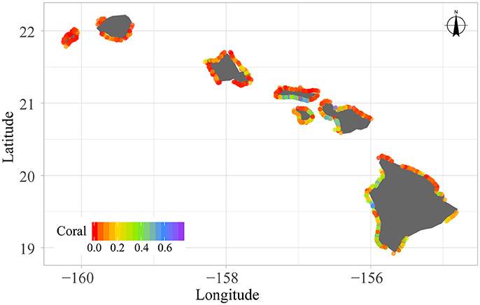
Figure 3. In situ percent coral cover for 717 reef fish surveys conducted around the main Hawaiian Islands between 2012 and 2015.

All covariates were first checked for correlation (Pearson's r > 0.5). Correlations were found within each suite of oceanographic variables (e.g., mean SST was correlated with other temporally averaged metrics of SST, but not with any other oceanographic variable) as well as within the full suite of substrate complexity measures (Supplementary Table S2). While island-scale wave energy and SST have been shown to be strongly correlated at other spatial scales (Heenan et al., 2016), we did not find this pattern at the site-level. Retaining the most straightforward variable from each set of correlated variables resulted in the list of variables in the first column of Supplementary Table S3. In order to account for multi-collinearity, variance inflation factors (VIFs) were calculated for the remaining set while removing variables with the highest VIF in a stepwise manner until all VIFs < 5. We initially retained coral cover and turf algae cover despite their high negative correlation and allow the VIF calculation to decide which should be dropped first (Supplementary Table S3). The result was a set of 17 non-collinear variables retained for further consideration (last column of Supplementary Table S3 and first column of Table 2).

TABLE 2

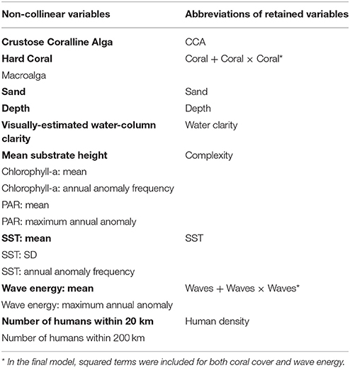
Table 2. List of all non-collinear variables, with those in bold retained in the final model, and their abbreviations in the manuscript.

To address the non-linear relationship between human population density and reef fish biomass and following Nadon et al. (2012) and Williams et al. (2015), we used log(no. of humans) for our human population density variables. Furthermore, we include a squared term for coral cover and wave energy (i.e., coral + coral² and wave + wave²) to capture the known non-linear relationship between those drivers and reef fish biomass (Friedlander et al., 2003; Williams et al., 2015; Heenan et al., 2016).

We model fish biomass, yi, at the site-level, using a hierarchical linear model. This allows us to account for the multi-scale, nested structure of our data observations as well as our model parameters. Specifically, our model structure has site i nested in sector j, nested in island k, nested in region, such that

$\begin{array}{cc}\text{log}(\text{yi})~\text{normal}({\text{XiB}}_{\text{j}[\text{i}]},{\sigma }_{\text{y}}^{\text{2}})& (1)\end{array}$

for i = 1,…,N sites, where X is the n x P matrix of P predictors including the intercept (i.e., the first column is a column of 1's), and Bj is a vector of regression coefficients, such that XiB_j[i] is the linear regression model for site i in sector j.

We then nest B_j[i] within the island-level such that

$\begin{array}{cc}{\text{B}}_{\text{j}[\text{i}]}~\text{multivariate normal}({\text{MB}}_{\text{k}[\text{j}],}\Sigma {\text{B}}_{\text{k}[\text{j}]})& (2)\end{array}$

for j = 1,…,J sectors, and k = 1,…,K islands, where B is the J x P matrix of regression coefficients and B_j[i] is a vector of length P of regression coefficients for sector j; MB_k[j] is a vector of length P corresponding to the means of the distribution of the intercept and slope of all sectors in island k; and ΣB_k[j] is the P x P matrix of the covariances between the intercept and slopes for island k.

We then nest MB_k[j] within the regional-level (i.e., the main Hawaiian Is- lands) such that

$\begin{array}{cc}{\text{MB}}_{\text{k}[\text{j}]}~\text{multivariate normal}(\text{MB},\Sigma \text{B})& (3)\end{array}$

where ΣB is the P x P matrix of the regional-level (i.e., overall) covariances between the intercept and slopes.

Following Gelman and Hill (2007) and Barnard et al. (2000), we then model the covariance matrices using a scaled inverse-Wishart distribution, the over-all effect of which, is to set a uniform distribution between −1 and +1 on the individual correlation parameters of the covariance matrix (See Supplementary Text S2). Finally, because our regression coefficients are nested, we only have to give a prior to the regional level such that each regression coefficient in the vector MB is given a normal distribution with a mean of 0 and a variance of 10. All scaling parameters (see Supplementary Text S2) are given a uniform prior distribution between 0 and 1.

Model Fitting and Analysis

We first ran our model with the full list of non-collinear variables (first column of Table 2) using Markov Chain Monte Carlo (MCMC) algorithms in JAGS (Just Another Gibbs Sampler; Plummer, 2003) called from R (R Core Team, 2016) using the R package, rjags (Plummer, 2011). We ran three parallel chains of length 500,000 with a burn-in period of 400,000 and 1/10 thinning leaving a total of 10,000 samples from the MCMC history to be used in calculating Bayesian credible intervals for all parameters. We then followed Gelman and Hill (2007) as our framework in deciding which drivers to include in the final model. Briefly, we removed those drivers that did not have a significant effect on fish biomass (i.e., its 95% confidence intervals overlapped with zero for at least 80% or 20 out of the 25 analyzed sectors) and only retained those (Table 2) that had a clear effect.

We then re-ran our final model with the final list of retained drivers (final column of Table 2) using the same MCMC specifications above. Convergence was assessed by: (i) inspecting traceplots of all estimated parameters and ensuring that all chains were well-mixed and stable and (ii) calculating Gelman-Rubin statistics (Gelman and Rubin, 1992)—all were close to 1, indicating that variance within and between chains were close to equal. Our JAGS code can be found in Supplementary Text S3. Posterior predictive checks were used to assess model fit (i.e., a step was added in each MCMC iteration to simulate data based on our model's posterior predictive distribution, which we then compare to our observed dataset).

Goodness of fit was evaluated using Bayesian p-values, which are based on comparing the discrepancies between observed and simulated data. Bayesian p-values for the mean (p = 0.50) and standard deviation (p = 0.61) were both close to 0.5, indicating that differences between observed and simulated data are likely due to chance. Furthermore, we checked full model residuals as well as individual covariate residuals against predicted values to verify they are normally-distributed, uncorrelated and homoscedastic.

Next, we checked predictive power at both the sector and site-level. At the site-level, the model appeared to show some bias at the extremes (Supplementary Figures S2A,B), but the model's predictions of sector-level total (Figure 4) and herbivorous (Supplementary Figure S3) reef fish biomass (median: black dots; gray rectangles: 95% Bayesian credible intervals) agree with observed levels of fish biomass (red diamond and whiskers). We consider this model performance to be appropriate since we summarize our simulation of biomass baselines at the sector-level. For all other results, we report 66% Bayesian credible intervals to express “likely” outcomes, following the United Nations – Intergovernmental Panel on Climate Change's guidance for expressing uncertainty (Mastrandrea et al., 2010).

FIGURE 4

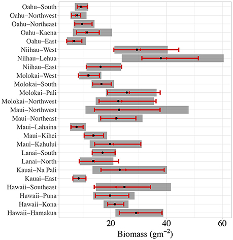
Figure 4. Observed (red whiskers) vs. predicted (gray rectangles) 95% quantiles for sector-level total reef fish biomass.

To estimate the impact of human population density on both total and herbivorous fish biomass throughout Hawaii, we first used our final model to estimate the effect of human population density—given the variation in fish biomass that is attributable to spatial differences in environmental habitat and oceanographic drivers—at each location. Then, we added a step in each MCMC iteration to simulate fish biomass baselines, by setting human population levels to its minimum value found in the main Hawaiian Islands (in order to keep our predictions within the range of our data). For the 2010 U.S. Census (United States Census Bureau, 2010) on which our human population data is based, the minimum population level within 20 km of a fish survey site was 117 humans, located in the Niihau-Lehua sector (Figure 1). Because this is done within the MCMC, these estimates of biomass baselines incorporate the model uncertainty in the effect of human population density on fish biomass. In addition, each MCMC iteration is coded to calculate the percentage increase between present-day and baseline levels of fish biomass—i.e., the percentage change from present-day fish biomass if human impacts were minimized (i.e., set to the minimum level within the current dataset)—and is termed “percent recovery potential” here.

Results

A total of 11 drivers were found to have a significant effect and thus retained in the final model for both the herbivorous and total reef fish analyses (Table 2 including abbreviations). Scatterplots of each variable vs. log total reef fish biomass can be found in Supplementary Figures S4A–I (and Supplementary Figures S5A–I for log herbivorous reef fish biomass). For each driver, and for each analysis (herbivorous and total reef fish biomass), the model provided estimates of driver coefficients for multiple levels: sector, island, and region. The regional-scale (i.e., overall) effect of all drivers were largely similar for total and herbivorous reef fish (Figure 5; Supplementary Table S4). The consistency of these results is not surprising given that the correlation between site-level total and herbivorous reef fish biomass was high (Pearson's r = 0.81); nevertheless because of interest from the local coral reef management community, we provide results from both analyses. Drivers with a positive effect on fish biomass were: CCA, Complexity, Depth, and Water Clarity. Drivers with a negative effect on fish biomass were: Human Density, Sand, and SST. Coral and Waves exhibited non-linear relationships with fish biomass (positive with Coral and Waves, negative with Coral x Coral and Waves x Waves). Finally, for the remainder of this article, we focus our results and discussion on our analysis of total reef fish biomass. All outputs for our herbivorous reef fish analysis can be found in the Supplementary Materials.

FIGURE 5

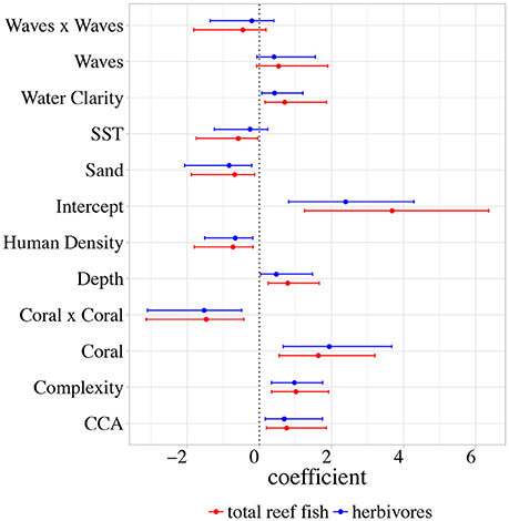
Figure 5. Region-scale (i.e., overall) effect of all drivers on total (red) and herbivorous (blue) reef fish log biomass in our hierarchical model for the main Hawaiian Islands. Mean (circle) and 66% Bayesian Credible Intervals (whiskers) are shown for each driver.

At lower, nested spatial scales (i.e., islands, sectors), spatial variation in driver effects was more apparent (Figure 6; Supplementary Figures S6A–K for total reef fish; Supplementary Figures S7A–L for herbivores). For example, the median sector-level effect of human density on total reef fish log biomass ranged from −0.18 in Hawaii-Kona to −0.46 in Niihau-Lehua (Figure 6). In contrast to human density, other drivers had relatively consistent effects. For example, the coefficient for wave energy (Supplementary Figure S6J) was relatively consistent across sectors and islands (only ranging between 0.22 and 0.25 despite site-level, mean wave energy ranging between 0.43 and 35.5 kW m⁻¹). The means of all island-level coefficient estimates are shown as light gray bars (See Supplementary Tables S5A,B for means and credible intervals).

FIGURE 6

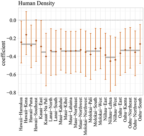
Figure 6. Sector-level effect (vertical whiskers) of human density on total reef fish log biomass in our hierarchical model for the main Hawaiian Islands. The mean (diamond) effect and 66% Bayesian Credible Intervals (whiskers) are shown for each sector. Island-level mean effects are also shown (gray horizontal bars).

Since the effect of human density is negative for all sectors (Figure 6), we see the model's median prediction of baseline biomass to always be greater than the median of present-day fish biomass for each sector (Figure 7; Supplementary Figure S8 for herbivores). Among sectors, however, there is considerable variation in the difference between the present-day and baseline biomass distributions, such that some sectors are considerably more different from baseline biomass than others. The proportional difference between these distributions is what we call “percent recovery potential” here (i.e., difference between present-day and baseline biomass as a proportion of present-day biomass; Figure 8; Supplementary Figure S9 for herbivores). Estimated baseline biomass and percent recovery potential are also displayed spatially in Figures 9, 10 (and for herbivores in Supplementary Figures S10, S11). For those interested in absolute, rather than proportional change in fish biomass, bar graphs (Supplementary Figure S12) and maps (Supplementary Figure S13) for both total and herbivorous reef fish are also provided.

FIGURE 7

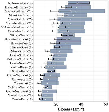
Figure 7. Sector-level model predictions of present-day (black whiskers) vs. baseline (blue rectangles) biomass for total reef fish in the main Hawaiian Islands. Means and 66% Bayesian Credible Intervals are shown. Baseline biomass is calculated by setting human density to its present-day minimum across all fish-survey sites.

FIGURE 8

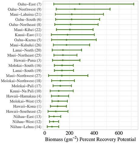
Figure 8. Sector-level percent recovery potential (i.e., difference between model-predicted present-day and baseline biomass as a proportion of present-day biomass) for total reef fish in the main Hawaiian Islands. Means and 66% Bayesian Credible Intervals are shown.

FIGURE 9

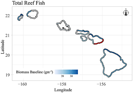
Figure 9. Map of sector-level, mean baseline biomass for total reef fish in the main Hawaiian Islands. Sectors with limited data are shown in red.

Discussion

Overall, our analysis provides two potential lenses with which the heterogeneity of coral reef fishery systems in the main Hawaiian Island can be understood. Our biomass baseline estimates highlight areas that have the greatest capacity to support reef fish biomass, given multiple habitat and oceanographic drivers and after removing the effect of human population density. This approach reveals considerable spatial variability in the natural carrying capacity of reef fish throughout the archipelago. The sector with the greatest baseline biomass (Niihau-Lehua) could support more than three times as much total reef fish biomass as the sector with the lowest baseline biomass (Kauai-East) (Figures 7, 9). And for herbivorous fish (Supplementary Figures S8, S10), this difference was even greater – the sector with the highest ability to support herbivorous reef fish (Maui-Northwest) could support ten times as much herbivorous biomass as the sector with the lowest baseline herbivorous fish biomass (Kauai-East). For total reef fish (Figure 9), the north coasts of Niihau, Maui, Molokai, and Hawaii have the greatest biomass baselines across all sectors. On the other hand, the four sectors with the greatest herbivorous fish biomass baselines are found on Maui, with the north coasts of Molokai, Niihau, and Kauai also having appreciable capacities to support herbivorous fish (Supplementary Figure S10).

An alternate perspective with which the variation in reef fish assemblages can be assessed is to consider which areas have the greatest capacity for recovery. Here, we defined recovery potential as the proportional increase in fish biomass after minimizing the effects of human density (i.e., percent recovery potential). While our simulation of minimizing human population density shows an increase from present-day to baseline biomass across all sectors, some sectors appear to be more sensitive to this reduction than others. For example, total reef fish biomass (Figures 8, 10) in Oahu-East was predicted to be able to experience a 280% increase from present-day levels if human impacts could be minimized. On the other hand, Niihau-Lehua was only predicted to have a 57% recovery potential. For herbivorous reef fish, the percent recovery potential was even greater (Supplementary Figures S9, S11), ranging from a minimum of 287% (Niihau-Lehua) to a maximum of 1764% (Oahu-Northwest). Overall, areas with the highest percent recovery potential for total reef fish are located throughout all of Oahu, as well as in the Maui-Lahaina and Maui-Kihei sectors (Figure 10). For herbivores (Supplementary Figure S11), the northern coast of Oahu as well as all of Maui island, especially the Maui-Kihei sector, had the greatest percent recovery potential.

FIGURE 10

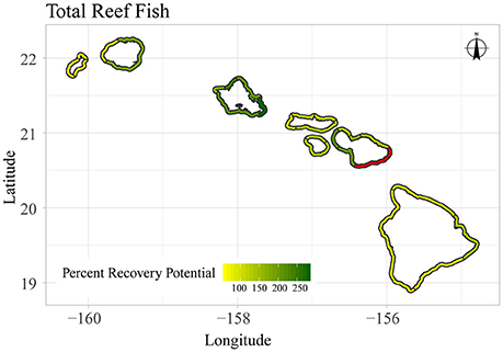
Figure 10. Map of sector-level, mean percent recovery potential for total reef fish biomass in the main Hawaiian Islands. Sectors with limited data are shown in red.

The two perspectives we provide here, baseline biomass and recovery potential, however, do not have to be mutually exclusive criteria for designing an overall management plan for the main Hawaiian Islands. Through its creation of multi-use ocean zoning plans and the delineation of different marine zones for different uses, MSP has the ability to implement multiple management objectives across time and space (Crowder and Norse, 2008; Day, 2008). Environmental management objectives can be broadly divided into conservation (e.g., preservation of areas that are near-pristine) and restoration (e.g., revival of areas with high recovery potential) activities (Hobbs et al., 2009). Specifically, sectors such as Niihau-Lehua, could be highly valued (e.g., for tourism purposes or as source of spillover into adjacent areas) due to the fact that they have a high baseline biomass and because their present-day biomass already closely matches their baseline. Areas like this could be prioritized for conservation management strategies aimed at preventing human impacts that cause biotic and abiotic changes to the system. On the other hand, sectors with high recovery potential (e.g., Oahu-East, Northwest, South, and Northeast as well as Maui-Lahaina and Kihei) could be prioritized for restoration purposes. In contrast to conservation-focused management activities, areas with high recovery potential would benefit instead from restoration management actions designed to reverse biotic and abiotic changes and promote recovery toward a previous state (Hobbs et al., 2009).

In the absence of a reliable time series that predates coral reef degradation, we estimated baseline biomass through the use of spatial gradients, along a spectrum of most to least impacted reef areas in the region. Such an approach is not without caveats. The ability for an ecosystem to rebound from the present-day state to a baseline, requires that several other assumptions be met. For example, if present-day environmental conditions are not able to fully account for the observed current state of an ecosystem due its historical trajectory (i.e., hysteresis) or if other processes such as larval recruitment patterns and successional dynamics are not fully understood, then the recovery pathway may not simply be the reverse of the decline pathway (Diaz and Rosenberg, 2008). Furthermore, if the ecosystem has been tipped past a threshold into an alternative stable state threshold, recovery to its original state may not even be possible (Hughes et al., 2017). In light of these caveats, our estimate of recovery potential should be considered as a robust estimate of current levels of depletion from baselines, but actual recovery trajectory remains uncertain. Although we could not address these issues related to ecosystem recovery, we did address at least one critical challenge by providing estimates at a scale that is relevant to local managers.

Our ability to bring previous island-level analyses (Williams et al., 2015) to the sub-island (sector) scale stems from our use of a hierarchical analytical framework, which considers the effects of drivers as being spatially-nested and operating on multiple scales. At the regional-scale, the strongest drivers of fish biomass in the main Hawaiian Islands were from coral cover and complexity (Figure 5). Coral had a negative non-linear relationship with fish biomass (positive for Coral and negative for Coral x Coral); other studies (Williams et al., 2015; Heenan et al., 2016) have indicated that intermediate levels of coral cover tend to have the highest levels of fish biomass. One possible explanation of this nonlinear effect of coral cover is that increasing coral cover and associated substrate complexity provide refugia for reef fish against predation (Beukers and Jones, 1998; Almany, 2004), but as coral cover increases to become the dominant benthic organism, this may eventually lead to the exclusion of other benthic organisms (e.g., turf, endolithic algae) that are important food sources for certain functional guilds (Wismer et al., 2009). Although increasing coral cover can help to build and maintain high complexity reef habitats, the two variables were not correlated at the site-level for our dataset and are likely mediating different dynamics for different groups of reef fish (e.g., changes in coral cover vs. complexity will likely have different effects on corallivores vs. other groups) (Emslie et al., 2014). Wave power produced a similar non-linear effect (positive for Waves and negative for Waves x Waves). This has also been demonstrated previously on this scale (Friedlander et al., 2003; Rodgers et al., 2010), and one potential mechanism for this may have to do with the availability of algae and accumulation of detritus in areas of intermediate wave forcing (Crossman et al., 2001).

In general, the model coefficients for human density tended be more variable among sectors than those for environmental drivers (Figure 6 vs. Supplementary Figures S6A–K). In our analysis, we transformed both fish biomass and human density so that their relationship would be linear on the log-log scale (Supplementary Figures S4E, S5E), which means that their coefficients should be interpreted as elasticities, i.e., a human density coefficient of X means that a 10% increase in human density results in a X*10% decrease in fish biomass, regardless of the human density of the sector. In other words, a 10% increase of human density will have a larger effect on fish biomass on Niihau (4.1%) than on Oahu (3.3%; Figure 6). However, as Oahu's population is so large, the effect of minimizing human population density there corresponds to a large total effect on fish biomass. Therefore, in contrast to Niihau's sectors, the biomass baselines for Oahu are quite different from their present-day biomass levels (Figure 7). Overall, the linear, log-log relationship between fish biomass and human population density that we find in this study, and corresponding interpretation of the human density coefficient as elasticities, is consistent with other studies (Nadon et al., 2012; Heenan et al., 2016).

As is becoming increasingly recognized, the effects of local human populations are highly context- and scale-dependent, and in some cases other, related, metrics such as distance to markets are stronger drivers of coral reef fisheries conditions (Cinner and McClanahan, 2006; Brewer et al., 2009; Cinner et al., 2013). The exact mechanism by which human population density negatively affects standing reef fish biomass was not explicitly tested here, although others have suggested this to be related to a combination of fishing pressure and/or degraded water quality from land development (Mora et al., 2011). Thus, independently of any change in human populations in the main Hawaiian Islands, managing the human footprint as it relates to these ecosystem stressors will be crucial to ensuring the sustainability of coral reef fisheries.

In order to address the diversity of human activities that impact coral reef ecosystems, advocates of MSP suggest a hierarchical management approach, whereby larger (e.g., national) levels of management provide context for nested, lower (e.g., local) levels (Gilliland and Laffoley, 2008). Coral reefs, in turn, are hierarchically-structured ecosystems, lending themselves to hierarchical analyses (MacNeil et al., 2009); yet rarely has this analytical approach been explicitly applied toward guiding coral reef MSP efforts. Our study should highlight the applicability and utility of hierarchical analyses to providing management-relevant input to MSP. Specifically, our analytical framework allowed for the characterization of biophysical and human impact drivers operating at multiple levels, as well as the downscaling of coral reef ecosystem benchmarks to a scale relevant to local managers. This allowed for the identification of areas with the greatest scope for recovery (e.g., heavily impacted areas with high background oceanic productivity and high-quality habitat) and conversely, areas which, because of poor habitat quality and other factors, are not likely to be able to ever support high levels of fish biomass. Furthermore, by taking a Bayesian approach, our estimates of baseline biomass and recovery potential incorporated the uncertainty of all modeled parameters, including the effect of humans. Uncertainty is a common denominator in resource management and conservation, with scientists asked to quantify it and managers asked to buffer against it. Being transparent about the uncertainty around modeled predictions is critical to effective collaboration between science and management.

MSP has the potential to reconcile the multiple economic, social, and environmental demands placed on coral reef ecosystems (Gilliland and Laffoley, 2008). Controlling for multiple habitat, oceanographic, and human factors in the way we have done makes it possible to reveal the natural heterogeneity of coral reef ecosystems as well as how they have been affected by human impacts. Our estimates of baseline biomass and recovery potential can guide MSP efforts as managers integrate multiple sources of information and begin to delineate management actions across heterogeneous stretches of coasts and seascapes. Ultimately the decision of which management objectives to prioritize is a societal choice, but these decisions should be informed by scientific input. By providing spatially-explicit, locally-relevant benchmarks (Crowder and Norse, 2008; Day, 2008), scientists can guide MSP efforts and enable managers to make informed decisions of how and where to prioritize their efforts.

Author Contributions

KG, MD, AH, and IW: conceived the research, shaped the analyses, and interpreted the results; KG: analyzed the data; MD and KG: developed the model; KG: wrote the main manuscript, with MD, AH, and IW providing considerable edits. JG: provided oceanographic data; IW and RB: coordinated and fundraised for research cruises and data collection. All authors provided critical feedback and helped with finalizing the manuscript

Funding

Data collection and research were supported by NOAA's Coral Reef Conservation Program (http://coralreef.noaa.gov) and the NOAA Pacific Islands Fisheries Science Center.

Conflict of Interest Statement

The authors declare that the research was conducted in the absence of any commercial or financial relationships that could be construed as a potential conflict of interest.

Acknowledgments

We thank the members of the Coral Reef Ecosystem Program's fish team for their tireless efforts in collecting reef fish monitoring data around the main Hawaiian Islands as well as the dedicated officers and crews of the NOAA Ships Hi‘ialakai and Oscar Elton Sette for providing safe and productive platforms for our research teams. We also thank Tomoko Acoba for GIS support with this project, Amanda Dillon for graphics support, and Hal Koike for initial discussions on the framing of this analysis for Hawaii Division of Aquatic Resources. Finally, we thank the NOAA Coral Reef Conservation Program and the Pacific Islands Fisheries Science Center for supporting this research. The contents in this manuscript are solely the opinions of the authors and do not constitute a statement of policy, decision, or position on behalf of NOAA or the U.S. Government.

Supplementary Material

The Supplementary Material for this article can be found online at: https://www.frontiersin.org/articles/10.3389/fmars.2018.00162/full#supplementary-material

References

Almany, G. R. (2004). Does increased habitat complexity reduce predation and competition in coral reef fish assemblages? Oikos 106, 275–284.

Google Scholar

Ayotte, P., Mccoy, K., Williams, I., and Zamzow, J. (2011). Coral Reef Ecosystem Division Standard Operating Procedures: Data Collection for Rapid Ecological Assessment Fish Surveys. Pacific Islands Fisheries Science Center. Administrative Report H-11-08, 24

Google Scholar

Barnard, J., McCulloch, R., and Meng, X.-L. (2000). Modeling covariance matrices in terms of standard deviations and correlations, with application to shrinkage. Stat. Sin. 10, 1281–1311.

Google Scholar

Bellwood, D. R., and Choat, J. H. (1990). A functional analysis of grazing in parrotfishes (family Scaridae), the ecological implications. Environ. Biol. Fishes 28, 189–214.

Google Scholar

Beukers, J. S., and Jones, G. P. (1998). International association for ecology habitat complexity modifies the impact of piscivores on a coral reef fish population. Oecologia 114, 50–59. doi: 10.1007/s004420050419

CrossRef Full Text | Google Scholar

Brewer, T. D., Cinner, J. E., Green, A., and Pandolfi, J. M. (2009). Thresholds and multiple scale interaction of environment, resource use, and market proximity on reef fishery resources in the Solomon Islands. Biol. Conserv. 142, 1797–1807. doi: 10.1016/j.biocon.2009.03.021

CrossRef Full Text | Google Scholar

Chabanet, P., Ralambondrainy, H., Amanieu, M., Faure, G., and Galzin, R. (1997). Relationships between coral reef substrata and fish. Coral Reefs 16, 93–102. doi: 10.1007/s003380050063

CrossRef Full Text | Google Scholar

Cinner, J. E., and McClanahan, T. R. (2006). Socioeconomic factors that lead to overfishing in small-scale coral reef fisheries of Papua New Guinea. Environ. Conserv. 33, 73–80. doi: 10.1017/S0376892906002748

CrossRef Full Text | Google Scholar

Cinner, J. E., Huchery, C., Darling, E. S., Humphries, A. T., Graham, N. A., Hicks, C. C., et al. (2013). Evaluating social and ecological vulnerability of coral reef fisheries to climate change. PLoS ONE 8:e74321. doi: 10.1371/journal.pone.0074321

PubMed Abstract | CrossRef Full Text | Google Scholar

Cinner, J. E., Huchery, C., MacNeil, M. A., Graham, N. A., McClanahan, T. R., Maina, J., et al. (2016). Bright spots among the world's coral reefs. Nature 535, 416–419. doi: 10.1038/nature18607

PubMed Abstract | CrossRef Full Text | Google Scholar

Coral Reef Ecosystem Program: Pacific Islands Fisheries Science Center (2007). Coral Reef Monitoring Program: Stratified Random Surveys (StRS) of Reef Fish, Including Benthic Estimate Data of the U.S. Pacific Reefs Since. NOAA Natl Centers Environ Information Unpunblished dataset [2012–2015]. Available online at: https://inport.nmfs.noaa.gov/inport/item/24447

Crossman, D. J., Choat, J. H., Clements, K. D., Hardy, T., and McConochie, J. (2001). Detritus as food for grazing fishes on coral reefs. Limnol. Oceanogr. 46, 1596–1605. doi: 10.4319/lo.2001.46.7.1596

CrossRef Full Text | Google Scholar

Crowder, L., and Norse, E. (2008). Essential ecological insights for marine ecosystem-based management and marine spatial planning. Mar Policy. 32, 772–778. doi: 10.1016/j.marpol.2008.03.012

CrossRef Full Text | Google Scholar

Cvitanovic, C., Hobday, A. J., Kerkhoff, L., Van Wilson, S. K., and Dobbs, K. (2015). Improving knowledge exchange among scientists and decision- makers to facilitate the adaptive governance of marine resources : a review of knowledge and research needs. Ocean Coast. Manag. 112, 25–35. doi: 10.1016/j.ocecoaman.2015.05.002

CrossRef Full Text | Google Scholar

D'agata, S., Mouillot, D., Wantiez, L., Friedlander, A. M., Kulbicki, M., and Vigliola, L. (2016). Marine reserves lag behind wilderness in the conservation of key functional roles. Nat. Commun. 7:12000. doi: 10.1038/ncomms12000

PubMed Abstract | CrossRef Full Text | Google Scholar

Day, J. (2008). The need and practice of monitoring, evaluating and adapting marine planning and management-lessons from the Great Barrier Reef. Mar Policy. 32, 823–831. doi: 10.1016/j.marpol.2008.03.023

CrossRef Full Text | Google Scholar

Diaz, R. J., and Rosenberg, R. (2008). Spreading dead zones and consquences for marine ecosystems. Science 321, 926–929. doi: 10.1126/science.1156401

PubMed Abstract | CrossRef Full Text | Google Scholar

Ellison, A. (1996). An introduction to Bayesian inference for ecological research and environmental decision-making. Ecol. Appl. 6, 1036–1046. doi: 10.2307/2269588

CrossRef Full Text | Google Scholar

Emslie, M. J., Cheal, A. J., and Johns, K. A. (2014). Retention of habitat complexity minimizes disassembly of reef fish communities following disturbance: a large-scale natural experiment. PLoS ONE 9:e105384. doi: 10.1371/journal.pone.0105384

PubMed Abstract | CrossRef Full Text | Google Scholar

Friedlander, A. M., and DeMartini, E. E. (2002). Contrasts in density, size, and biomass of reef fishes between the northwestern and the main Hawaiian islands: the effects of fishing down apex predators. Mar. Ecol. Prog. Ser. 230, 253–264. doi: 10.3354/meps230253

CrossRef Full Text | Google Scholar

Friedlander, A. M., Brown, E. K., Jokiel, P. L., Smith, W. R., and Rodgers, K. S. (2003). Effects of habitat, wave exposure, and marine protected area status on coral reef fish assemblages in the Hawaiian archipelago. Coral Reefs 22, 291–305. doi: 10.1007/s00338-003-0317-2

CrossRef Full Text | Google Scholar

Friedlander, A. M., Stamoulis, K. A., Kittinger, J. N., Drazen, J. C., and Tissot, B. N. (2014). “Understanding the Scale of Marine Protection in Hawai'i: From Community-Based Management to the Remote Northwestern Hawaiian Islands,” in Advances in Marine Biology, 1st Edn. Vol. 69, eds M. L. Johnson and J. Sandell (London, UK: Elsevier Ltd), 153–203.

Google Scholar

Froese, R., and Pauly, D. (2016).Editors. FishBase. Available online at: www.fishbase.org

Game, E. T., McDonald-Madden, E., Puotinen, M. L., and Possingham, H. P. (2008). Should we protect the strong or the weak? Risk, resilience, and the selection of marine protected areas. Conserv Biol. 22, 1619–1629. doi: 10.1111/j.1523-1739.2008.01037.x

PubMed Abstract | CrossRef Full Text | Google Scholar

Gelman, A., and Hill, J. (2007). Data Analysis Using Regression and Multilevel/Hierarchical Models. New York, NY: Cambridge University Press.

Google Scholar

Gelman, A., and Rubin, D. B. (1992). Inference from iterative simulation using multiple sequences. Stat. Sci. 7, 457–472. doi: 10.1214/ss/1177011136

CrossRef Full Text | Google Scholar

Gilliland, P. M., and Laffoley, D. (2008). Key elements and steps in the process of developing ecosystem-based marine spatial planning. Mar Policy. 32, 787–796. doi: 10.1016/j.marpol.2008.03.022

CrossRef Full Text | Google Scholar

Gove, J. M., Williams, G. J., McManus, M. A., Heron, S. F., Sandin, S. A., Vetter, O. J., et al. (2013). Quantifying Climatological Ranges and Anomalies for Pacific Coral Reef Ecosystems. PLoS ONE 8:e61974. doi: 10.1371/journal.pone.0061974

PubMed Abstract | CrossRef Full Text | Google Scholar

Graham, N. A., Jennings, S., MacNeil, M. A., Mouillot, D., and Wilson, S. K. (2015). Predicting climate-driven regime shifts versus rebound potential in coral reefs. Nature 518, 94–97. doi: 10.1038/nature14140

PubMed Abstract | CrossRef Full Text | Google Scholar

Gray, A. E., Williams, I. D., Stamoulis, K. A., Boland, R. C., Lino, K. C., Hauk, B. B., et al. (2016). Comparison of reef fish survey data gathered by open and closed circuit SCUBA divers reveals differences in areas with higher fishing pressure. PLoS ONE 11:e0167724. doi: 10.1371/journal.pone.0167724

PubMed Abstract | CrossRef Full Text | Google Scholar

Green, A. L., and Bellwood, D. R. (2009). Monitoring Functional Groups of Herbivorous Reef Fishes as Indicators of Coral Reef Resilience - A Practical Guide for Coral Reef Managers in the Asia Pacific Region. IUCN working group on Climate Change and Coral Reefs. IUCN, Gland.

Google Scholar

Hatcher, B., and Larkum, A. (1983). An experimental analysis of factors controlling the standing crop of the epilithic algal community on a coral reef. J. Exp. Mar. Biol. Ecol. 69, 61–84. doi: 10.1016/0022-0981(83)90172-7

CrossRef Full Text | Google Scholar

Hay, M. E., Colbum, T., and Downing, D. (1983). Spatial and temporal patterns in herbivory on a Caribbean fringing reef: the effects on plant distribution. Oecologia 58, 229–308. doi: 10.1007/BF00385227

PubMed Abstract | CrossRef Full Text | Google Scholar

Heenan, A., and Williams, I. D. (2013). Monitoring herbivorous fishes as indicators of coral reef resilience in American Samoa. PLoS ONE 8:e79604. doi: 10.1371/journal.pone.0079604

PubMed Abstract | CrossRef Full Text | Google Scholar

Heenan, A., Ayotte, P., Gray, A., Lino, K., McCoy, K., Zamzow, J., et al. (2012). Pacific Reef Assessment and Monitoring Program. Data Report: Ecological Monitoring−2013 – Reef Fishes and Benthic Habitats of the Main Hawaiian Islands, American Samoa, and Pacific Remote Island Areas. 2014. Pacific Islands Fisheries Science Center, PIFSC Data Report, DR-14-003, 112.

Heenan, A., Hoey, A. S., Williams, G. J., and Williams, I. D. (2016). Natural bounds on herbivorous coral reef fishes. Proc. R. Soc. B Biol. Sci. 283:1716. doi: 10.1098/rspb.2016.1716

PubMed Abstract | CrossRef Full Text | Google Scholar

Heenan, A., Williams, I. D., Acoba, T., DesRochers, A., Kosaki, R. K., Kanemura, T., et al. (2017). Long-term monitoring of coral reef fish assemblages in the Western central pacific. Sci. Data 4:170176. doi: 10.1038/sdata.2017.176

PubMed Abstract | CrossRef Full Text | Google Scholar

Hobbs, R. J., Higgs, E., and Harris, J. A. (2009). Novel ecosystems: implications for conservation and restoration. Trends Ecol. Evol. 24, 599–605. doi: 10.1016/j.tree.2009.05.012

PubMed Abstract | CrossRef Full Text | Google Scholar

Hughes, T. P., Barnes, M. L., Bellwood, D. R., Cinner, J. E., Cumming, G. S., Jackson, J. B. C., et al. (2017). Coral reefs in the Anthropocene. Nature 546, 82–90. doi: 10.1038/nature22901

PubMed Abstract | CrossRef Full Text | Google Scholar

Li, N., Cheung, K. F., Stopa, J. E., Hsiao, F., Chen, Y.-L., Vega, L., et al. (2016). Thirty-four years of Hawaii wave hindcast from downscaling climate forecast system reanalysis. Ocean Model. 100, 78–95. doi: 10.1016/j.ocemod.2016.02.001

CrossRef Full Text | Google Scholar

MacNeil, M. A., Graham, N. A. J., Cinner, J. E., Wilson, S. K, Williams, I. D, Maina, J., et al. (2015) Recovery potential of the world's coral reef fishes. Nature 520, 341–344. doi: 10.1038/nature14358

PubMed Abstract | CrossRef Full Text | Google Scholar

MacNeil, M. A., Graham, N. A., Polunin, N. V., Kulbicki, M., Galzin, R., Harmelin-Vivien, M., et al. (2009). Hierarchical drivers of reef-fish metacommunity structure. Ecology 90, 252–264. doi: 10.1890/07-0487.1

PubMed Abstract | CrossRef Full Text | Google Scholar

Mastrandrea, M. D., Field, C. B., Stocker, T. F., Edenhofer, O., Ebi, K. L., Frame, D. J., et al. (2010). Guidance Note for Lead Authors of the IPCC Fifth Assessment Report on Consistent Treatment of Uncertainties. Intergovernment Panel Climate Change. Available online at: http://www.ipcc.ch

McClanahan, T. R., Graham, N. A., Calnan, J. M., and MacNeil, M. A. (2007). Toward pristine biomass: reef fish recovery in coral reef marine protected areas in Kenya. Ecol. Appl. 17, 1055–1067. doi: 10.1890/06-1450

PubMed Abstract | CrossRef Full Text | Google Scholar

McClanahan, T. R., Maina, J. M., Graham, N. A. J., and Jones, K. R. (2016). Modeling reef fish biomass, recovery potential, and management priorities in the Western Indian Ocean. PLoS ONE 11:e0154585. doi: 10.1371/journal.pone.0154585

CrossRef Full Text | Google Scholar

McCoy, K., Heenan, A., Asher, J., Ayotte, P., Gorospe, K., Gray, A., et al. (2015). Pacific Reef Assessment and Monitoring Program. Data Report : Ecological Monitoring : Reef Fishes and Benthic Habitats of the Main Hawaiian Islands, Northwestern Hawaiian Islands, Pacific Remote Island Areas, and American Samoa. 2016. Pacific Islands Fisheries Science Center, PIFSC Data Report, DR-16-002, 94

Google Scholar

McNie, E. C. (2007). Reconciling the supply of scientific information with user demands: an analysis of the problem and review of the literature. Environ. Sci. Policy. 10, 17–38. doi: 10.1016/j.envsci.2006.10.004

CrossRef Full Text | Google Scholar

Mellin, C., MacNeil, M. A., Cheal, A. J., Emslie, M. J., and Caley, M. J. (2016). Marine protected areas increase resilience among coral reef communities. Ecol. Lett. 19, 629–637. doi: 10.1111/ele.12598

PubMed Abstract | CrossRef Full Text | Google Scholar

Mora, C., Aburto-Oropeza, O., Ayala-Bocos, A., Ayotte, P. M., Banks, S., Bauman, A. G., et al. (2011). Global human footprint on the linkage between biodiversity and ecosystem functioning in reef fishes. PLoS Biol. 9:e1000606. doi: 10.1371/journal.pbio.1000606

PubMed Abstract | CrossRef Full Text | Google Scholar

Mora, C., Graham, N. A. J., and Nyström, M. (2016). Ecological limitations to the resilience of coral reefs. Coral Reef. 35, 1271–1280. doi: 10.1007/s00338-016-1479-z

CrossRef Full Text | Google Scholar

Nadon, M. O., Baum, J. K., Williams, I. D., McPherson, J. M., Zgliczynski, B. J., Richards, B. L., et al. (2012). Re-creating missing population baselines for Pacific reef sharks. Conserv. Biol. 26, 493–503. doi: 10.1111/j.1523-1739.2012.01835.x

PubMed Abstract | CrossRef Full Text | Google Scholar

Pandolfi, J. M., Connolly, S. R., Marshall, D. J., and Cohen, A. L. (2011). Projecting coral reef futures under global warming and ocean acidification. Science 333, 418–422. doi: 10.1126/science.1204794

PubMed Abstract | CrossRef Full Text | Google Scholar

Plummer, M. (2003). “JAGS: A program for analysis of Bayesian graphical models using Gibbs sampling,” in Proceedings of the 3rd International Workshop on Distributed Statistical Computing.

Plummer, M. (2011). rjags: Bayesian graphical models using MCMC. R package version 3–5.

R Core Team (2016). R: A Language and Enviroment for Statistical Computing. Vienna. Available online at: https://www.r-project.org/

Robinson, J. P., Williams, I. D., Edwards, A. M., McPherson, J., Yeager, L., Vigliola, L., et al. (2017). Fishing degrades size structure of coral reef fish communities. Glob. Chang. Biol. 23, 1009–1022. doi: 10.1111/gcb.13482

PubMed Abstract | CrossRef Full Text | Google Scholar

Rodgers, K. S., Jokiel, P. L., Bird, C. E., and Brown, E. K. (2010). Quantifying the condition of Hawaiian coral reefs. Aquat. Conserv. Mar. Freshw. Ecosyst. 20, 93–105. doi: 10.1002/aqc.1048

CrossRef Full Text | Google Scholar

Sandin, S. A., and Williams, I. (2010). Trophic Classifications of Reef Fishes from the Tropical U.S. Pacific (Version 1.0). Scripps Institution of Oceanography Technical Report. Scripps Institution of Oceanography, San Diego, CA.

Google Scholar

Steneck, R. S. (1988). “Herbivory on coral reefs: a synthesis,” in Proceedings of the 6th International Coral Reef Symposium (Townsville), 37-49.

United States Census Bureau (2010). Census. 2010. Available online at: http://www.census.gov/2010census/data/

University of Hawaii Social Science Research Institute (2017). Coral Bleaching Recovery Plan: Identifying Management Responses to Promote Coral Recovery in Hawaii. Available online at: https://dlnr.hawaii.gov/reefresponse/files/2016/09/CoralBleachingRecoveryPlan_final_newDARlogo.pdf

Wedding, L. M., Lecky, J., Gove, J. M., Walecka, H. R., Donovan, M. K., Williams, G. J., et al. (2017). Advancing the integration of spatial data to map human and natural drivers on coral reefs. PLoS ONE 13:e0189792. doi: 10.1371/journal.pone.0189792

PubMed Abstract | CrossRef Full Text | Google Scholar

Williams, I. D., Baum, J. K., Heenan, A., Hanson, K. M., Nadon, M. O., and Brainard, R. E. (2015). Human, oceanographic and habitat drivers of central and western Pacific coral reef fish assemblages. PLoS ONE 10:e0120516. doi: 10.1371/journal.pone.0120516

PubMed Abstract | CrossRef Full Text | Google Scholar

Wismer, S., Hoey, A. S., and Bellwood, D. R. (2009). Cross-shelf benthic community structure on the Great Barrier Reef: relationships between macroalgal cover and herbivore biomass. Mar. Ecol. Prog. Ser. 376, 45–54. doi: 10.3354/meps07790

CrossRef Full Text | Google Scholar