Long-Term Mean Circulation of the Baltic Sea as Represented by Various Ocean Circulation Models

Introduction

Understanding of ocean climate requires, inter alia, knowledge of long-term variability in transports of volume, heat, salt, and matter by highly varying currents. The Baltic Sea as a semi-enclosed sea in Northern Europe covers an area of approximately 420,000 km² and is subdivided into several basins (see Figure 1) which formed after the last glaciation. With an average depth of only 54 m the Baltic Sea is strongly responding to atmospheric influences. It is characterized by an intense freshwater supply from the difference between precipitation and evaporation over the sea surface and the inflow from a variety of surrounding rivers. For the period 1970 to 1999 the total runoff into the Baltic Sea including Kattegat amounts to 15,500 m³ s⁻¹ (calculated from Meier and Döscher, 2002, c.f. Bergström and Carlsson, 1994) with an error of about ± 600 m³ s⁻¹ (Omstedt and Nohr, 2004). Another significant feature are salt water exchanges with the World Ocean via the North Sea in the west. This leads to a gradient in salinity from west to northeast and hence strong stratification in the Baltic Sea interior. Atmospheric winds strongly influence both salt water inflows into this very shallow and tide-less sea and coastal upwelling. In turn, precipitation and wind depend on the large-scale atmospheric circulation which is characterized by, e.g., the North Atlantic Oscillation (NAO) and related storm tracks.

FIGURE 1

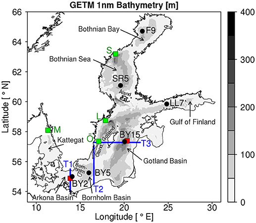
Figure 1. Locations of the used monitoring stations for the assessment of temperature and salinity (black dots) and current velocities (red squares) as well as the analyzed transects (blue lines) in the Baltic Sea. The background color (gray shading) shows the bathymetry [m] from the GETM-1 nm-run. Exemplary stations for atmospheric wind data comparison are shown as green squares. See text for further information.

The first diagnostic model of the horizontal summer circulation in the Baltic Sea which based upon the geostrophic balance was applied by Sarkisyan et al. (1975). With the help of a three-dimensional (3D) circulation model based upon the primitive equations Lehmann and Hinrichsen (2000) calculated the mean circulation and its stability during four consecutive years from 1992 to 1995. Despite the large variability in atmospheric forcing, like wind and sea level pressure, they found rather stable annual mean circulation patterns with only some inter-annual variations in the magnitude of the basin-wide cyclonic gyre transports.

Also with diagnostic models Stigebrandt (1987) and Elken (1996) calculated the interleaving of saline water into the eastern Gotland Basin deep water. They found maxima in 60–65 and 90–110 m depth, respectively, indicating small- and medium-size inflows ventilating the halocline and a secondary maximum at the bottom of the Gotland Basin indicating Major Baltic Inflows (MBIs) (Matthäus and Franck, 1992). Similar results were reported from 3D circulation modeling (Meier and Kauker, 2003). Approximately, these transports below the Ekman layer form the lower branch of the estuarine circulation in the Baltic Sea.

Further analysis of the wind-driven and thermohaline (or estuarine) circulation of the Baltic Sea was performed by Döös et al. (2004), who calculated the overturning stream function on a transect along the axis of the Baltic Sea in temperature, salinity or density coordinates instead of depth and estimated the residence time with Lagrangian particles released in Öresund, Great Belt and at the mouth of the river Neva. According to Döös et al. (2004) the residence time of particles released in the entire water volume of the Baltic Sea amounts to 26–29 years.

A useful tool to quantify time scales of water masses and to describe the circulation is the concept of age (e.g., Deleersnijder et al., 2001), that has been introduced into 3D Baltic Sea models, e.g., by Andrejev et al. (2004a,b) for the Gulf of Finland, by Meier (2005, 2007) for the entire Baltic Sea, and by Myrberg and Andrejev (2006) for the Gulf of Bothnia. Using a passive tracer for the age, which is the time elapsed since a water parcel left the sea surface, Meier (2005) quantified the sensitivity of the Baltic deep water ventilation with respect to changes in freshwater supply, wind speed and sea level amplitude in Kattegat. He found that changes of fresh- or saltwater inflow or low-frequency wind longer than the turnover time scale may cause the Baltic Sea to drift into a new state with significantly changed salinity but with only slightly altered stability and deep water ventilation. The vertical overturning circulation is partially recovered. By contrast, long-term changes of the high-frequency wind affect mixing and by that deep water ventilation significantly.

From these earlier studies, Elken and Matthäus (2008) draw a schematic view of the large-scale circulation in the Baltic Sea including entrainment, diffusion and upwelling. However, recent observations suggest that probably the understanding of the overturning circulation has to be revised because lateral mixing and mixing at the sloping bottom are one order of magnitude larger than vertical mixing in the stratified interior (Holtermann and Umlauf, 2012; Holtermann et al., 2012). Hence, mixing parameterizations in ocean circulation models need to be revised, especially if the driving processes are not properly resolved.

The focus of the present study is on the assessment of state-estimates of the Baltic Sea generated by various ocean circulation models with differing vertical coordinates, differing mixing parameterizations as well as distinct atmospheric and hydrological forcing in the light of how good physical conditions and processes are reproduced and how suitable the models are for detailed investigations in the Baltic Sea region. For this purpose, we have selected three state-of-the-art ocean circulation models, namely the General Estuarine Transport Model (GETM; Burchard and Bolding, 2002; Gräwe et al., 2015, 2016), the Rossby Centre Ocean model (RCO; Meier et al., 2003; Meier, 2007), and the Modular Ocean Model (MOM; Neumann et al., 2002; Griffies, 2004). These models are originally developed for different purposes and have been used previously in numerous process and climate studies for the Baltic Sea and other coastal seas. Their capability to simulate the evolution, variability, and vertical profiles of temperature and salinity as well as mean large-scale circulation patterns and volume transports for the present-day time period from 1970 through 1999 is investigated qualitatively and quantitatively.

In this regard, we assess the model results with respect to observations and also have a closer look into the atmospheric wind forcing which is used for driving the ocean models. Since there are no long-term observational datasets with high spatial and temporal resolution, we rely on existing reanalyses. However, even the resolution of most state-of-the-art reanalysis datasets, like for example ERA-Interim (Dee et al., 2011), is still too coarse to drive high-resolution regional ocean models (e.g., Meier et al., 2011). Therefore, regional climate models are used to perform a downscaling of the global reanalyses (Samuelsson et al., 2011; Geyer, 2014).

Note, that we do not perform a model intercomparison due to the different model setups, grid resolutions, vertical coordinates, parameterizations of sub-grid scale processes as well as atmospheric and hydrological forcing. Hence, we can only speculate about the causes for differences in model results. As all models have been calibrated to monitoring data of temperature and salinity, the aim of the study is to analyze uncertainties in the modeling of the resulting mean circulation, which is of great importance for climate studies. Although model results are strictly speaking not comparable, we will show that nevertheless interesting conclusions for the modeling of the mean circulation can be drawn. Thus, our intention is to compare state estimates, rather than models following Pätsch et al. (2017) for the North Sea or Myrberg et al. (2010) for the Gulf of Finland on shorter time scales. For instance, in the latter study it was concluded that the performance of the models was generally satisfactory although simulated vertical profiles of temperature and salinity were biased compared to observations particularly in the eastern Gulf of Finland.

The manuscript is organized as follows. In section Methods the data base including brief descriptions of the used ocean circulation models and their setups, the observational datasets, the statistical evaluation measures, and the experimental strategy are described. An evaluation of the model simulations together with the observations is presented in section Results. This assessment contains vertical profiles of temperature and salinity at specific representative monitoring stations in the Baltic Sea as well as statistical time series analyses of temperature and salinity at different depths. The dynamics represented by the models are investigated by an analysis of patterns of horizontal surface current and volume transport. Further, mean current velocities and volume transports at selected cross sections perpendicular to the estuarine flow are analyzed and statistics of current velocities at two monitoring stations are performed. That section is completed by an evaluation of the atmospheric wind data. In section Discussion causes for the differences in the mean circulation between the models are discussed. Section Summary, Conclusions, and Outlook summarizes and concludes the present study and reveals prospects for future investigations.

Methods

Ocean Circulation Models

For the present assessment three state-of-the-art ocean circulation models were investigated. The General Estuarine Transport Model (GETM; Burchard and Bolding, 2002; Hofmeister et al., 2010; Gräwe et al., 2015, 2016) is a three-dimensional baroclinic open source model with hydrostatic and Boussinesq assumptions and was mainly developed for shallow sea applications. GETM uses terrain-following vertically adaptive coordinates and applies an Arakawa C-grid for horizontal coordinates with free-slip lateral boundary conditions. The used mixing parameterization in vertical direction was a two-equation k-ε turbulence model coupled to an algebraic second-moment closure. Lateral diffusion of momentum, salinity and temperature was carried out along the model layers with a harmonic Smagorinsky diffusivity and a turbulent Prandtl number of three. The model version used in this study had 50 vertical layers and used a horizontal resolution of 1 nautical mile (nm). The minimum thickness of vertical layers was limited to 50 cm. The same held for the thickness of the surface layer to have a better representation/computation of the surface fluxes. The model domain comprised the Baltic Sea and was a reduced version of the setup of Gräwe et al. (2015). Atmospheric forcing data were taken from the coastDat2 hindcast dataset (Geyer, 2014), which is a regional downscaling of the global NCEP/NCAR reanalysis (Kalnay et al., 1996) with spectral nudging, and which has a spatial resolution of about 24 km (0.22°). River runoff was based on HELCOM (2015). Output of the present GETM version were daily mean data along selected transects and at individual stations, but also full 3D monthly means of temperature, salinity, currents and heat/salt fluxes. For the present study, data output on the vertically adaptive coordinates had been interpolated to a regular vertical grid with 2 m resolution.

The Rossby Centre Ocean model (RCO) is a Bryan-Cox-Semtner primitive equation circulation model with a free surface (Killworth et al., 1991) and a lateral open boundary in the Kattegat (Meier et al., 2003), which was originally intended for large-scale ocean simulations of the Baltic Sea. Subgrid-scale mixing was parameterized using a turbulence closure scheme of the k-ε type with flux boundary conditions to include the effect of a turbulence enhanced layer due to breaking surface gravity waves and a parameterization for breaking internal waves (Meier, 2001). No explicit horizontal diffusion was applied whereas a harmonic parameterization of the horizontal viscosity was chosen (Meier, 2007). In vertical direction level coordinates were used and in horizontal direction simulations were based on an Arakawa B-grid with no-slip lateral boundary conditions. In this study simulations were used from a conventional setup (Eilola et al., 2011; Löptien and Meier, 2011) and an assimilation/reanalysis setup by Liu et al. (2017, see also Liu et al., 2013, 2014) which in the following will be referred to as RCO and RCO-A, respectively. In RCO-A all temperature and salinity profiles from the Swedish Ocean Archive (SHARK; http://sharkweb.smhi.se) available during 1970–1999 were assimilated using the ensemble optimal interpolation method (Liu et al., 2017). Detailed numbers of the used observed profiles per sub-basin and year can be found in Liu et al. (2017, their Figure 2). Note, that the data assimilation integrates the information from both model and observations to provide the best estimation of ocean state. But nevertheless RCO-A differs from observations as the used assimilation system is not perfect and measurements for assimilation are neither available continuously nor do they cover the entire model domain. Further, RCO-A utilized the same ocean model as in RCO simulations except that the bathymetry of Słupsk Channel was deeper for RCO-A than for RCO. This methodical deepening in RCO-A served as a tool for optimizing salinity in the central and northern Baltic Sea. However, it turned out that the impact of deepening the Słupsk Channel on salinity was negligible. Both model setups had a vertical resolution of 3 m and a horizontal resolution of 2 nm. As atmospheric forcing regionalized ERA40 data (Uppala et al., 2005) using the Rossby Centre Atmosphere model version 3 (RCA3; see Meier et al., 2011; Samuelsson et al., 2011) were used. Due to the known underestimation of the wind speed in RCA3 compared to observations the simulated wind speed was corrected using the gustiness of the wind (Höglund et al., 2009; Meier et al., 2011). The river runoff was based on Bergström and Carlsson (1994). The data used here had a two-daily time resolution.

The Modular Ocean Model (MOM version 5.1) is a circulation model which was also developed for large-scale ocean simulations (e.g., Pacanowski and Griffies, 2000; Griffies, 2004) and had been adapted to the Baltic Sea with an explicit free surface, an open boundary condition with respect to the North Sea, and freshwater riverine input (e.g., Neumann et al., 2017). The used mixing parameterizations are the K profile parameterization (KPP; Large et al., 1994) in vertical direction and the Smagorinsky scheme (Smagorinsky, 1963) in horizontal direction. MOM used vertical level coordinates on z*-layers and an Arakawa B-grid in the horizontal plane with no-slip lateral boundary conditions. In this study the horizontal resolution was 3 nm and the vertical layer thickness varied between 0.5 m at the surface and about 2 m at depths greater than approximately 50 m. Similar as in the GETM simulations, coastDat2 data were taken as atmospheric forcing and HELCOM data as river runoff data. The original time resolution of the data at single stations was hourly. Full 3D data fields had monthly resolution.

For a consistent assessment the different horizontal and vertical grid resolutions of the used ocean models needed to be considered carefully. In order to evaluate wind-driven and baroclinic circulation patterns and volume transports as well as the bathymetry of the entire Baltic Sea, we used a uniform horizontal grid resolution of 2 nm for all models, i.e., current velocities from RCO simulations remained on their original grid, whereas velocities simulated by GETM and MOM were interpolated to that grid. The calculation of the volume transports was then done by multiplying the velocities and the interpolated velocities, respectively, by the zonal and meridional distances of the 2-nm grid. Differences of horizontal surface current patterns between RCO-A and each of the other models were determined by subtracting the magnitudes of the respective velocity vectors. For the analysis of zonal or meridional currents through transects we interpolated current speeds simulated by MOM on z*-layers to a regular vertical resolution of 2 m. For RCO in both setups and GETM with their regular vertical grids no adjustment was needed.

Observations

Temperature and Salinity

For assessing the physical conditions simulated by the selected ocean circulation models we took the Baltic Environmental Database (BED; http://nest.su.se/bed) of the Baltic Nest Institute, Stockholm, into account which is a collection of quality controlled hydrographic and biogeochemical data around the Baltic Sea. In the present study post-processed monthly averages were used which cover the time period from 1970 to 2008 (Gustafsson and Rodriguez-Medina, 2011). These data were available every 5 m near the surface, every 10 m between 20 and 100 m depth, and for stations reaching even deeper data were predominantly available every 25 m. At these standard depths observations of temperature, salinity, and many other parameters were gathered which lie between 1 m above and 1 m below that depth. For the present study we considered data from the monitoring stations BY2 in the Arkona Basin (55.0°N, 14.1°E), BY5 at Bornholm Deep (55.3°N, 16.0°E), BY15 at Gotland Deep (57.3°N, 20.0°E), LL7 in the Gulf of Finland (59.9°N, 24.8°E), SR5 in the Bothnian Sea (61.1°N, 19.6°E), and F9 in the Bothnian Bay (64.7°N, 22.1°E). Their locations are illustrated in Figure 1 as black dots. The selected stations cover conditions in the southern, the central, and the northern Baltic Sea and differ primarily in the influence of salt water inflows, thermal conditions due to insolation, and characteristics of currents. The average numbers of observations per depth used for temperature and salinity at these monitoring stations are ~1,500 at BY2, ~4,250 at BY5, ~1,100 at BY15, ~640 at LL7, ~360 at SR5, and ~300 at F9. A detailed listing of samples per parameter, depth, and station is given in Gustafsson and Rodriguez-Medina (2011). Note, that the observed profiles assimilated into RCO-A are a sub-set of the BED database.

Current Velocity

For the evaluation of simulated current velocities we used measurements which were performed (a) with an Acoustic Doppler Current Profiler (ADCP) at the Arkona monitoring station of the Marine Environment Observation Network (MARNET) and (b) with a subsurface mooring close to Gotland Deep. Their locations are shown as red squares in Figure 1. The Arkona station (54.9°N, 13.9°E) is operated since the year 2003 on behalf of the Federal Maritime and Hydrographic Agency of Germany (BSH) by the Leibniz Institute for Baltic Sea Research Warnemünde (IOW). It works autonomous and is equipped with a variety of instruments (Krüger, 2000). For the present study ADCP measurements of hourly current velocity were considered for the time period from 2005 through 2014.

These 10 years were also covered by GETM and MOM simulations whereas model runs of RCO-A and RCO were not available during that time. Therefore, a comparable 10-year time period from 1990 through 1999 was used for the statistical analysis of these models. For the comparison with the ADCP data model results had been taken from 3D fields at approximately the same location as the observations. Model results from GETM and MOM were only considered when observations were available. For RCO-A and RCO which do not cover the same time period, we shortened the 10-year time series by the length of the measurement gaps.

The Gotland mooring is deployed northeast of Gotland Deep (57.4°N, 20.3°E) and was equipped with current meters (Aanderaa RCM-7 and/or RCM-9). It measured temperature, current speed, and current direction with a sampling interval of 1 h. For this study we used daily averages of zonal and meridional currents at 204 m depth (Hagen and Feistel, 2004) for the years 2000 until the end of 2004. During these 5 years simulations were available for GETM, MOM, and RCO. Again, for RCO-A, we chose an equivalent 5-year time period, namely from 1995 through 1999, as the simulations of this model finished at the end of 1999. The respective depths from the simulations for the comparison with the mooring measurements were 204 m for GETM, 205 m for MOM, and 205.5 m for RCO-A and RCO. Datasets from the models were taken from 3D fields at the same location as the observations for GETM, RCO-A, and RCO. As the bathymetry in MOM is shallower than in the other models at the location of the mooring, the next wet grid point further west from the mooring was chosen which is located at 20.2°E.

Wind Velocity

For the estimation of how close the two atmospheric wind forcing datasets RCA3-ERA40 and coastDat2 are to reality, we compared them to wind measurements from 28 automatic stations along the Swedish coast for the time period from 1996 through 2008 (Höglund et al., 2009). The observations were available as hourly 10-minute averages. The temporal resolution of CoastDat2 was hourly whereas RCA3-ERA40 had only 3-hourly resolution. Hence, for a direct comparison of forcing and measured data, daily averages had been computed for the three datasets. In order to compare the station-based observations to the gridded reanalysis datasets, the nearest grid point away from land had been manually selected from the models for each station. Exemplary mean annual cycles of wind speed were investigated at the stations Skagsudde at the northern Bothnian Sea coast (63.2°N, 19.0°E), Landsort at the northwestern central Baltic coast (58.7°N, 17.9°E), Ölands Norra Udde at the northern tip of the island Öland (57.4°N, 17.1°E), and Måseskär at the eastern coast of the Skagerrak (58.1°N, 11.3°E). Their locations are shown in Figure 1 as green squares with abbreviations S (Skagsudde), L (Landsort), Ö (Ölands Norra Udde), and M (Måseskär).

Evaluation Measures

Taylor Diagram

The evaluation of simulated temperature and salinity included the use of Taylor diagrams (Taylor, 2001). A Taylor diagram combines standard deviation, Pearson correlation coefficient, and centered root mean square (RMS) difference in a single diagram. The Pearson correlation coefficient represents the similarity in pattern between the simulated and observed time series. It is depicted by straight lines which are related to the azimuthal angle. Values from 0 to 1 stand for no correlation up to 100% accordance. The standard deviation of each model time series was calculated relative to the standard deviation of the observations in order to allow a unified representation of the different model results in one Taylor diagram. This normalized standard deviation is proportional to the radial distance from the origin of the diagram. For results close to the arc with the relation of 1 between the standard deviations of simulated and observed time series, the pattern variations in the model are correct, i.e., they are of similar amplitude as in the observations. The centered RMS difference in the simulated time series is proportional to the distance from the intersection of that arc with the x-axis. A perfect agreement between model results and observations would be located directly at that intersection meaning that the correlation of both time series is highest and the RMS error in the model time series is lowest. For details the reader is referred to Taylor (2001).

Cost Function

As Taylor diagrams do not consider offsets of modeled and observed time series, a cost function as an additional statistical measure for the quality of the simulated results was taken into account. Following Eilola et al. (2011) this cost function (C) was computed for each model (i) from

$\begin{array}{ll}{C}_i=\left|\frac{M_i-B}{STD}\right|& (1)\end{array}$

with M_i and B being the monthly mean values of the individual models and of the BED validation data set, respectively, and STD being the standard deviation of the observations. The cost function values were calculated for each depth considered in the Taylor diagrams and assess the correspondence between simulations and observations as follows: 0 ≤ C < 1 represents good quality, 1 ≤ C < 2 represents reasonable quality, and all C ≥ 2 signify poor agreement. Hence, a good accordance occurs if the long-term mean of a model does not deviate more than plus or minus one standard deviation from the mean of the BED validation data.

Based on the statistical measures which are included in the Taylor diagrams, an extended cost function was computed. Here we took three terms into account for differences between mean values, standard deviations as well as the RMS error

$\begin{array}{l}C{M}_i=\frac{1}{3}\left(\left|\frac{M_i-B}{STD}\right|+\left|\frac{ST{D}_i-STD}{STD}\right|+\left|\frac{RMS{E}_i}{STD}\right|\right)\end{array}(2)$

Here, STD_i and RMSE_i are the standard deviation and the centered root mean square error of each model, respectively.

Experimental Strategy

In order to assess the quality of the ocean circulation models RCO (both in a conventional setup and an assimilation setup which is referred to RCO-A), GETM, and MOM (see section Methods) for application in the Baltic Sea, a 30-year time period from 1970 through 1999 was analyzed. We focused on the models' ability to simulate temperature and salinity as realistic as possible when compared to observations gathered in the BED validation dataset. This assessment included the investigation of vertical profiles as well as statistical time series analysis for different depths at certain monitoring stations in the Baltic Sea.

In a further step horizontal patterns of surface current velocities and depth-integrated volume transports as simulated by the different models for the entire Baltic Sea were assessed and compared to the reanalysis RCO-A. We also analyzed the vertical structure of simulated currents through three transects in the Baltic Sea. These transects were located in the Arkona Basin (from 53.8 to 55.5°N, at 13.9°E), at the western entrance of Słupsk Channel (from 54.5 to 57.1°N, at 16.6°E), and in the Gotland Basin (at 57.3°N, from 16.5 to 21.8°E). They are illustrated in Figure 1 as the blue lines T1, T2, and T3, respectively. The Słupsk transect T2 was exceptional in that its northern region between Sweden and Öland was only an open channel in the GETM simulations such that the northern and southern parts of this transect both contributed to the volume transport. In contrast, in RCO-A, RCO, and MOM the northern and southern part of the Słupsk transect were separated by a land connection between Sweden and the southern part of Öland such that only the southern part contributed to the entire volume transport. Hence, for calculation of the vertical profile of volume transport through T2 the entire transect was considered for GETM, but only the southern part of it for the other models.

Finally, current velocities measured by an ADCP and a mooring at two different monitoring stations were compared to the model results and the atmospheric wind forcing data driving the ocean models were analyzed.

Results

Temperature and Salinity at Monitoring Stations

Mean Profiles

Figure 2 shows the 30-year mean vertical profiles of temperature and salinity with their standard deviations at the six monitoring stations. Mean values and standard deviations were calculated from monthly averages of each year from 1970 through 1999, i.e., 360 data profiles were included for averaging. Mean temperatures at the considered stations cover a range from approximately 2 to 9.5°C with maximum standard deviations of close to 6°C near the sea surface. The temperature at about 0 to 20 m depth is well represented by all models at the stations BY5, BY15, and SR5. There the maximum deviations between each model mean and the observational mean are smaller than 1°C. However, the near-surface temperature fits also well at BY2 for RCO-A, RCO, and GETM whereas it is slightly overestimated by more than 1°C by MOM. At LL7 and F9 the near-surface temperature is underestimated by all models by up to 2°C.

FIGURE 2

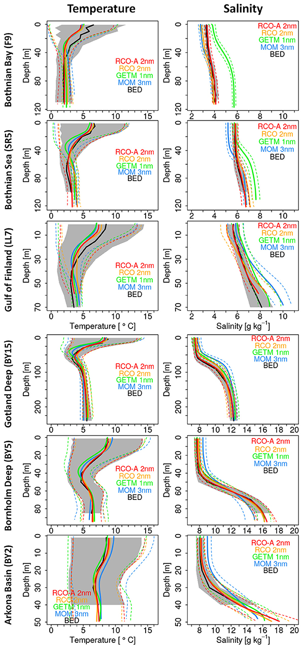
Figure 2. Thirty-year mean vertical profiles of sea temperature (left) and salinity (right) from BED observation data (black) and the ocean models RCO-A (red), RCO (orange) both with 2 nm horizontal resolution, GETM (green) with 1 nm resolution, and MOM (blue) with 3 nm resolution for the time period from 1970 through 1999. Results for the monitoring stations BY2 in the Arkona Basin, BY5 at Bornholm Deep, BY15 at Gotland Deep, LL7 in the Gulf of Finland, SR5 in the Bothnian Sea, and F9 in the Bothnian Bay are displayed from bottom to top. Mean values are illustrated by solid lines. Standard deviations are indicated by the gray-shaded area for the BED data and by the colored dashed lines for the models. The depth ranges are adjusted to the maximum water depth at each station and therefore differ for the individual stations. Note, that the value range for salinity is different for the southern and the northern stations.

The thermocline stretches on average from 20 to 40–60 m depth depending on each station. For most of the stations, the simulated thermocline by GETM and MOM lies somewhat higher (10 to 20 m closer to the sea surface) than in the BED validation data. Below the thermocline, RCO-A fits almost perfect to the observations at all stations, whereas RCO, GETM, and MOM slightly overestimate temperature by up to 1.5°C at the northern stations. At very large depths (like for BY15 and SR5), all models have standard deviations smaller than 1°C.

The 30-year mean vertical salinity profiles cover a range of approximately 3 to 9 g kg⁻¹ at the surface and 4 to 18 g kg⁻¹ at the bottom. At most of the stations the standard deviations of the BED data and the model simulations are predominantly much smaller than 1 g kg⁻¹. Exceptions are BY2 and LL7 as well as the bottommost depth range at BY5, where standard deviations are up to 3 g kg⁻¹ in maximum. Simulated mean salinity by RCO rarely exceeds the standard deviation of the BED dataset. This also holds for GETM at the southern stations, but at the northern stations GETM partly overestimates the observations by up to 2 g kg⁻¹ although the near-surface salinity is well reproduced. MOM salinity simulations deviate more often from the observed means and their standard deviations at all stations with maximum underestimation by 1 g kg⁻¹ at SR5 at the surface and maximum overestimation by 2 g kg⁻¹ at LL7 near the bottom.

In summary, simulated means by RCO partly exceed the range covered by the standard deviation of the BED validation data. Means simulated by GETM and MOM exceed the BED standard deviations more often than RCO at various depths, but GETM has an overall better agreement with the observations than MOM. The almost perfect agreement between RCO-A and BED profiles at the monitoring locations are expected as the observed profiles which were assimilated into RCO-A are a sub-set of the BED database.

Mean Seasonal Cycle

For Gotland Deep (BY15), which is the second deepest location in the Baltic Sea, we further assessed the model results at the sea surface in detail. Figure 3 shows the 30-year mean annual cycles of monthly sea surface temperature (SST) and sea surface salinity (SSS) with their standard deviations. The mean temperature stretches from approximately 1–3°C in March to 17–18°C in August. RCO overestimates the mean SST by 0.5 to almost 1.5°C from January to July with the maximum occurring in June. For August to December the RCO simulations are similar to those of RCO-A. GETM and MOM show a different behavior with underestimation of mean temperature by 0.5 to almost 1.5°C from November to March and an overestimation by 0.5–3°C from May to August. Thereby MOM simulations of mean temperature lie almost continuously within the observed standard deviation (except for June) while GETM simulations exceed the observed standard deviation from November to February as well as in June. Largest absolute differences between RCO-A and BED data amount to 0.5°C.

FIGURE 3

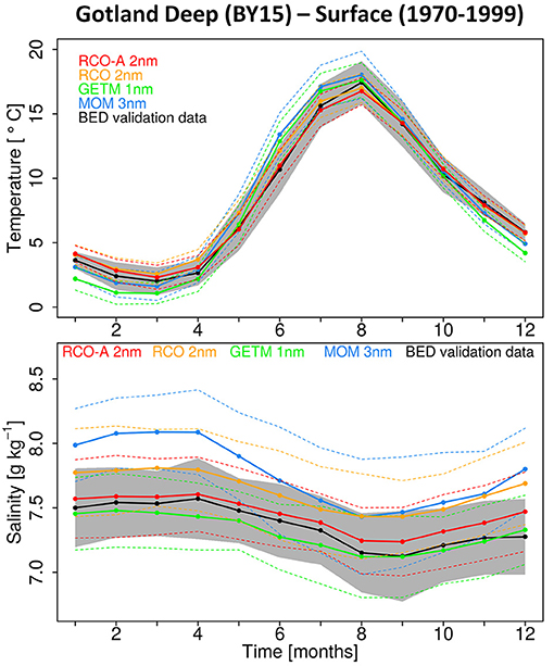
Figure 3. Thirty-year mean annual cycles of monthly sea surface temperature (top) and salinity (bottom) from BED observation data (black) and the ocean models RCO-A (red), RCO (orange), GETM (green), and MOM (blue) at the monitoring station Gotland Deep (BY15) for the time period from 1970 to 1999. Mean values are illustrated by solid lines. Standard deviations are indicated by the gray-shaded area for the BED data and by the colored dashed lines for the models.

The mean observed SSS shows only a weak annual cycle with values of approximately 7.1–7.6 g kg⁻¹ peaking in April and lowest values in September. GETM reproduces these values almost perfectly with a minor underestimation of about 0.1 g kg⁻¹ from January to August. The mean SSS simulated by RCO shows a comparable annual cycle as in the observations, but with a positive offset of about 0.2–0.4 g kg⁻¹. Hence, the RCO simulations lie approximately at the upper standard deviation of the BED validation dataset or slightly above it. MOM overestimates the mean observed SSS more than RCO, namely by about 0.3–1.1 g kg⁻¹, and shows an annual cycle with stronger magnitudes. The values only lie within the upper observed standard deviation from July to September and otherwise above it. Overall, the standard deviations of the BED validation data and the models are of similar magnitude. SSSs in RCO-A are slightly higher throughout the year by about 0.1–0.2 g kg⁻¹ than in the observations.

Interannual Variability

We further analyzed temperature and salinity in the deep water at BY15, which is approximately at 225 m depth in the models. Figure 4 shows time series of monthly mean values for 1970 through 1999. During this time period the observed bottom temperature varies between about 4 and 7°C with the minimum occurring from 1994 to 1995 and two maxima occurring in 1977 and 1998. The observed deep water salinity is lowest in 1993 with 10.9 g kg⁻¹ and highest in 1977 with 13.6 g kg⁻¹. For both temperature and salinity, RCO-A agrees very well with the BED data both in magnitude and variability. Sudden changes in temperature and salinity like for instance at the beginning of 1994 or 1998 are reproduced very realistically.

FIGURE 4

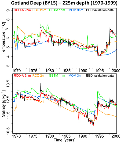
Figure 4. Monthly mean temperature (top) and salinity (bottom) from BED observation data (black) and the ocean models RCO-A (red), RCO (orange), GETM (green), and MOM (blue) at 225 m depth at Gotland Deep (BY15) for the years from 1970 to 1999.

The other models partly reproduce observed magnitudes very well, but do not show the strong variability which is visible in the BED and RCO-A data. RCO and GETM over- or underestimate temperature at 225 m depth from time to time by up to 1.5°C. MOM underestimates temperature almost continuously by about 0.5 to 2.5°C in maximum. Salinity at 225 m depth is predominantly underestimated by RCO and overestimated by GETM and MOM with maximum deviations from the observations of about 1 g kg⁻¹. The best accordance of models and observations occurs in the time period from 1983 through 1986 where GETM and MOM simulate the observed salinity decrease precisely.

Statistical Evaluation

In order to assess the capability of the single models to simulate the temporal evolution of temperature and salinity at various depths at each monitoring station within the 30-year time period, we applied Taylor diagrams and cost functions. The Taylor diagrams for temperature in Figure 5 show an overall similar distribution of near-surface values which lie accumulated close to the brown reference point (which has a normalized standard deviation of 1 and a correlation of 100%). This indicates the high quality of all simulations near the sea surface. The correlations of the SST time series even lie in general between 95 and 98%, the RMS errors are smaller than 0.3, and the normalized standard deviations for SST are closest to 1 at BY2, BY5, LL7, and F9.

FIGURE 5

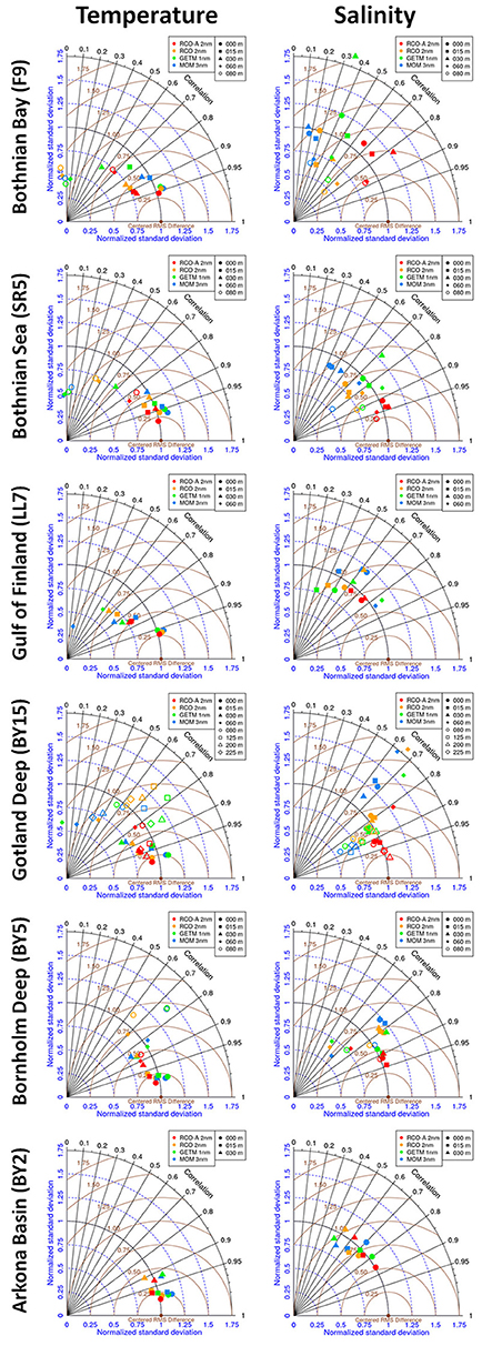
Figure 5. Taylor diagrams derived from monthly time series of sea temperature (left) and salinity (right) from 1970 to 1999 at particular standard depths at BY2 in the Arkona Basin, BY5 at Bornholm Deep, BY15 at Gotland Deep, LL7 in the Gulf of Finland, SR5 in the Bothnian Sea, and F9 in the Bothnian Bay. Correlation, normalized standard deviation, and centered RMS difference of the simulated time series from the ocean models RCO-A (red), RCO (orange), GETM (green), and MOM (blue) compared to the BED observation data are shown. Different plotting symbols refer to the single depths. See text for more details.

At larger depths the temperature correlations generally become worse and show a larger spread around the solid black arc, which represents a normalized standard deviation of 1. Moreover, the model results partly also show RMS errors greater than 1. The highest correlations always occur for RCO-A, the lowest predominantly for GETM or MOM.

The good reproduction of the near-surface temperature simulations is supported by the cost function in Figure 6. For all models and at all stations, the temperature cost function values at 0, 15, and 30 m depth lie between 0 and 1, which represents good quality. At larger depths the different capabilities of the individual models to simulate temperature become obvious. RCO-A has overall very low cost function values between 0 and 0.5, which emphasizes the excellent quality of this reanalysis dataset. For RCO, GETM, and MOM the temperature cost function below 30 m depth lies mainly between 0 and 1 and maximizes for all models at 80 m depth at BY15 and SR5. There, values are partly up to 2, which still represents reasonable quality.

FIGURE 6

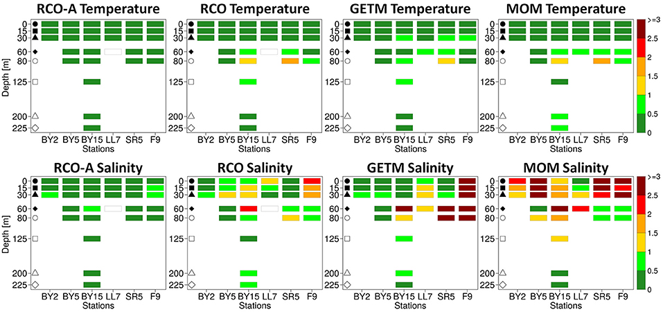
Figure 6. Cost function values derived from monthly time series of sea temperature (top) and salinity (bottom) from 1970 to 1999 at the six monitoring stations BY2, BY5, BY15, LL7, SR5, and F9. Results from the ocean models RCO-A, RCO, GETM, and MOM (from left to right) compared to the BED observation data are shown at the same depths as illustrated in the Taylor diagrams in Figure 5. The symbols in the left part of each diagram refer to the depth-dependent plotting symbols from the Taylor diagrams. Blank bins for RCO-A and RCO at LL7 and 60 m depth are due to missing data of these models at this location. See text for more details.

For salinity the Taylor diagrams and cost function values reveal stronger differences between the assessed models. RCO-A stands out at almost all stations with highest correlations over all depths and the smallest spread of the values around the normalized standard deviation of 1. The respective cost function values are predominantly smaller than 0.5, which underlines the very good accordance of reanalyzed salinity in RCO-A with the BED dataset.

The statistics of the salinity simulations by RCO and GETM are almost comparable to each other with RCO revealing an overall slightly better quality than GETM. Their correlations lie predominantly between 50 and 90%. Most deviations from the normalized standard deviation of 1 are about ±0.25 and RMS errors lie between 0.4 and 0.9. The cost function values lie predominantly between 0 and 1.5, but also reveal some shortcomings of these two models in simulating salinity at certain depths and stations.

Compared to the other models, salinity is represented worst by MOM. This arises from the predominantly low correlations in the Taylor diagrams (which mainly lie below 80%), the strong deviations from the normalized standard deviation of 1 (values up to about 0.7), and the high RMS errors (0.5 up to 1.3). Similarly, the cost function shows poor agreement (values greater than 2) at a variety of depths for the six monitoring stations. An interesting feature is that salinity simulations by MOM seem to be better at larger depths than toward the surface.

The above findings are also confirmed by the mean cost function value CM over all stations and all depths for temperature and salinity (Equation 2, see Table 1). Also for this mean cost function RCO-A reveals lowest values. RCO and GETM are mid-table and MOM reveals highest values and hence lowest quality. Overall, the mean cost function values for temperature have a smaller spread than those for salinity for the three model simulations and the reanalysis.

TABLE 1

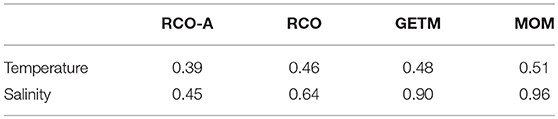
Table 1. Mean cost function values CM for temperature and salinity determined from Equation 2 for the ocean models RCO-A, RCO, GETM, and MOM.

Mean Circulation

Horizontal Surface Current Patterns

For the assessment of the mean circulation of the entire Baltic Sea there currently exists still no comprehensive data product from measurements which could be involved. Therefore, we chose RCO-A with assimilated data as a reference for the following analyses even though this model does not reflect the true reality. Differences between model results which arise in the following underline the need for more long-term and large-scale current measurements. Figure 7 shows the 30-year mean values of the surface current velocity averaged over the upper 10 m and of the volume transport integrated over the whole depth range (surface to bottom) as well as the used bathymetry of RCO-A. For the other models differences of these parameters from the results of RCO-A are illustrated. Large areas of the Baltic Sea surface reveal surface velocities between 0 and 3 cm s⁻¹ from RCO-A. Maxima of up to almost 28 cm s⁻¹ appear in the Kattegat, values of up to 17 cm s⁻¹ and 13 cm s⁻¹ in the Øresund and Great Belt, respectively, and there are several channel-like regions throughout the whole Baltic Sea with enhanced current velocities of about 5–8 cm s⁻¹ on average. Further conspicuous maxima occur for instance northwest of the island Bornholm, at the southern tip of the island Öland or approximately between Sweden and the Åland Islands.

FIGURE 7

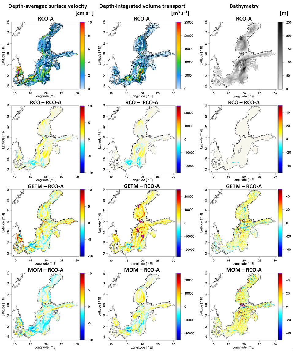
Figure 7. Thirty-year mean surface velocity averaged from the Baltic Sea surface down to 10 m depth (left) and volume transport integrated from the surface to the bottom (middle) as well as the used model bathymetry (right) for the years 1970 through 1999. In the top panels absolute values from the model RCO-A are displayed. Arrows show the direction of velocity and transport, respectively, at every 5th model grid point. The panels below show the differences of the individual models RCO, GETM, and MOM from RCO-A, respectively. Values exceeding the maximum positive plotting range are drawn in purple.

The difference between the surface current pattern simulated by RCO and that simulated by RCO-A shows—when compared to the other models—relatively small deviations of about ±4 cm s⁻¹ in maximum and 0.2 cm s⁻¹ on average. GETM and RCO-A surface currents differ stronger throughout the whole Baltic Sea with −12 cm s⁻¹ as negative maximum and 25 cm s⁻¹ as positive maximum. The average deviation is 0.7 cm s⁻¹. The surface speed difference between MOM and RCO-A reveals predominantly negative values, i.e., MOM simulates mainly smaller current speeds than RCO-A. The maximum negative and positive difference is about −10 cm s⁻¹ and 12 cm s⁻¹, respectively, and the average deviation is approximately −0.4 cm s⁻¹.

Horizontal Transport Patterns and Bathymetry

The depth-integrated volume transport simulated by RCO-A has values of 0–6,000 m³ s⁻¹ on average and maximizes in Gotland Basin (values of up to 39,000 m³ s⁻¹), Bornholm Basin (about 24,000 m³ s⁻¹), and Arkona Basin (about 14,000 m³ s⁻¹) with an almost closed counterclockwise gyre each. Further minor maxima appear at Landsort Deep, around the Åland Islands as well as in the northern Bothnian Sea. In general, the patterns of the depth-integrated volume transport for the other models are quite similar in the Gotland Basin but, again, the deviations from RCO to RCO-A are smallest throughout the whole Baltic Sea and largest differences occur for GETM. The pattern of the differences between RCO and RCO-A is comparable to the corresponding pattern seen for their surface velocity. Maximum positive deviations of about 12,000 m³ s⁻¹ and negative deviations of almost −17,000 m³ s⁻¹ occur around Słupsk Channel in the southern Baltic Sea. This is possibly mainly due to the fact that the bathymetry of Słupsk Channel is deeper for RCO-A than for RCO (see Figure 7). On average, the basin wide deviation of the depth-integrated volume transport of RCO-A and RCO is zero.

The depth-integrated volume transport simulated by GETM is significantly higher than that simulated by RCO-A. On average, the deviation is almost 4,000 m³ s⁻¹ throughout the whole Baltic Sea. Most negative deviations occur in Bornholm Basin with values of up to −13,000 m³ s⁻¹. The strongest positive deviations are found at Landsort Deep (~ 94,000 m³ s⁻¹), between Sweden and the Åland Islands (~ 80,000 m³ s⁻¹), in the northern Bothnian Sea (~ 52,000 m³ s⁻¹), at Gotland Deep (~ 42,000 m³ s⁻¹), and at the northern edge of Kattegat (~ 30,000 m³ s⁻¹). For MOM the deviations to RCO-A are again smaller than those from GETM to RCO-A with an average value of about 600 m³ s⁻¹. Most of the negative deviations occur in Bornholm Deep (maximizing in about −23,000 m³ s⁻¹) as well as in Gotland Basin. Positive deviations are found throughout the whole Baltic Sea and maximize in the Bothnian Sea, between Sweden and Gotland and at Słupsk Channel.

Local differences of depth-integrated volume transport do not necessarily result from differences in bathymetries. A direct coherence of bathymetry and volume transport occurs obviously along Słupsk Channel where volume transports simulated by RCO, GETM, and MOM differ from RCO-A. However, many other regions throughout the entire Baltic Sea which are characterized by strong volume transport differences coincide with small differences between model bathymetries (e.g., in Bornholm Basin, central Gotland Basin or in the southeastern Bothnian Sea). The other way around, big differences in the bathymetries of GETM or MOM versus RCO-A which occur for instance in the northeastern Gotland Basin and toward the Gulf of Finland are not characterized by very strong volume transport differences. And in the region between Sweden and the Åland Islands the bathymetry difference between GETM and RCO-A is smaller than that between MOM and RCO-A, but GETM shows much higher volume transport differences to RCO-A than MOM. Hence, the used bathymetries are individually adapted to the numerical solvers of each model for optimal representation of the physical conditions, and their patterns do not necessarily affect local current or volume transport patterns as these are compensated by the large-scale circulation.

Currents Through Transects

Figure 8 shows the mean current velocities through the three transects as simulated by the ocean circulation models. Positive values indicate eastward currents for Arkona and Słupsk transect (T1 and T2 in Figure 1) and northward currents for Gotland transect (T3 in Figure 1), respectively.

FIGURE 8

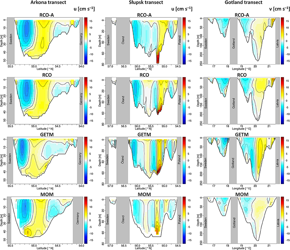
Figure 8. Mean current velocities orthogonal through Arkona transect (left), Słupsk transect (middle), and Gotland transect (right) for the time period from 1970 to 1999 for the models RCO-A, RCO, GETM, and MOM. Positive values denote eastward velocity for Arkona and Słupsk transect and northward velocity for Gotland transect. Isolines are drawn every 2 cm s⁻¹ (solid for positive values, dashed for negative values). Plotting range is ±17.3 cm s⁻¹. Note, that the shown transects cover different depth ranges.

The 30-year mean zonal velocity through the Arkona transect as simulated by all models shows the gyre-like structure which was already seen in the surface velocity and the depth-integrated volume transport in Figure 7. The current is westward directed (negative) in the northern part of the transect maximizing approximately between 5 and 15 m depth at about −9 cm s⁻¹ for RCO-A, RCO, and GETM and at about −7 cm s⁻¹ for MOM. In the middle part of the transect the current is eastward directed (positive) and almost constant over depth. However, for RCO-A and RCO a maximum of approximately 5 cm s⁻¹ appears at the surface whereas MOM simulates a maximum of almost 7 cm s⁻¹ below the westward directed current in the north. The southern region of the Arkona transect is characterized by a near-surface eastward current above a westward current as well as a westward coastline-current. Overall, the currents in the southern region are weaker than the gyre in the north. The center of this gyre lies at about 55 °N for RCO-A, RCO, and MOM, whereas it is slightly shifted toward the north by GETM.

The zonal current through Słupsk transect as simulated by RCO-A is predominantly westward (negative) in the northern part with a maximum of approximately −6 cm s⁻¹ near Öland. Approximately in the center between Öland and Poland currents are eastward (positive) with a strong maximum of almost 16 cm s⁻¹ within the pronounced Słupsk Channel (which has a depth of almost 80 m for RCO-A) and a weaker maximum of almost 6 cm s⁻¹ at the surface. Toward Poland the currents alternate. Principally, RCO, GETM, and MOM show comparable current patterns, but their westward directed northern current is interrupted by a weak eastward current at about 55.7°N each. RCO and GETM simulate partly stronger magnitudes than RCO-A and have their maximum at the entrance of the Słupsk channel between 50 and 60 m depth. MOM has the weakest current velocities throughout the whole Słupsk transect.

Meridional currents through Gotland transect reveal the gyre around Gotland Deep. Between Sweden and Gotland all models simulate predominantly southward (negative) current velocities, which are strongest for GETM (−9 cm s⁻¹) and RCO (−7 cm s⁻¹) and weakest for MOM (−3 cm s⁻¹). Between Gotland and Latvia the gyre structure is visible. In principle, the patterns simulated by RCO-A, RCO, and MOM are similar with MOM having the weakest magnitudes. GETM simulates the gyre with a slight shift to the east (such that it is centered directly at Gotland Deep over the whole depth range) and with stronger current velocities than the other models (values up to about ±5 cm s⁻¹).

Volume Transports Through Transects

Figure 9 shows the simulated 30-year mean vertical profiles of volume transport per depth interval which had been integrated horizontally along the three transects each. For the Arkona transect the vertical profiles of all models are very similar with maximum outflows from the Baltic Sea of about −1,900 to −1,700 m² s⁻¹ between 10 and 15 m depth and maximum inflows of about 1,300 to almost 1,600 m² s⁻¹ at around 40 m depth. Near the sea surface all models simulate inflows into the Baltic Sea with GETM having the strongest magnitudes.

FIGURE 9

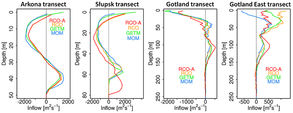
Figure 9. Vertical profiles of horizontally integrated flows per unit depth along Arkona, Słupsk, and Gotland transect as well as along the eastern part of the Gotland transect only (between Gotland and Latvia) as simulated by the ocean models RCO-A (red), RCO (orange), GETM (green), and MOM (blue) for the time period from 1970 to 1999. Note the different depth ranges of the individual transects.

At Słupsk transect the vertical structure of volume transport per depth interval is in principle comparable to that at Arkona transect, but due to the greater depth the maxima are located further down. Hence, the maximum outflow occurs at around 25 m depth for all models. The maximum inflow takes place near the surface as well as between 50 and 60 m depth for RCO, GETM, and MOM, but at about 70 m depth for RCO-A. The corresponding outflow magnitudes reach from almost −1,900 m² s⁻¹ for RCO-A to about −1,300 m² s⁻¹ for MOM. At the largest depths the inflow maximizes at about 1,600 m² s⁻¹ for RCO and almost 1,800 m² s⁻¹ for GETM.

Compared to Arkona and Słupsk transects the mean vertical profiles of volume transport per depth interval at Gotland transect have a different shape. Maximum outflow from the northern Baltic Sea takes place near the sea surface and inflow into the northern Baltic Sea occurs at depths below about 30 m for RCO, GETM, and MOM, but at depths below about 60 m for RCO-A. The maximum outflow ranges from almost −2,200 m² s⁻¹ for GETM to about −1,400 m² s⁻¹ for RCO-A and RCO. The inflow maximizes at about 300 m² s⁻¹ for RCO and GETM, almost 400 m² s⁻¹ for MOM, and over 500 m² s⁻¹ for RCO-A.

When only the eastern part of the Gotland transect is considered, i.e., the region between Gotland and Latvia, the vertical profiles differ from the profiles for the whole transect between the surface and approximately 110 m depth. Due to the exclusion of the western part of this transect, which is dominated by southward currents and hence outflow (see Figure 8), the Gotland East transect is characterized by inflow into the northern Baltic Sea over the whole depth range except for MOM. The stronger volume transport per depth interval between the surface and 50 m depth simulated by RCO-A, RCO, and GETM is due to the enhanced northward current at the eastern coast near Latvia, which is strongest pronounced in RCO near the sea surface. Therefore, RCO maximizes in about 1,200 m² s⁻¹ at the sea surface. At the same place RCO-A and GETM reveal inflows of about 400–500 m² s⁻¹ while MOM simulates maximum outflow of about −600 m² s⁻¹. The vertical profile of RCO is comparable to that by Meier and Kauker (2003, their Figure 13) even though they used a different horizontal resolution and showed total mean horizontally integrated transports (in m³ s⁻¹).

Table 2 summarizes the mean total volume transports through the Gotland transect calculated from the vertical profiles shown in Figure 9 by taking the vertical resolutions of the individual models into account and summing over depth. The outflow above the reversal depth of each profile has comparable values of about −30,000 m³ s⁻¹ for RCO, GETM, and MOM. In RCO-A a deeper located reversal depth coincides with a higher outflow of about −36,000 m³ s⁻¹. The inflow below the reversal depth is again similar for RCO, GETM, and MOM (approximately 17,000 m³ s⁻¹), but consequently higher for RCO-A (21,000 m³ s⁻¹). The corresponding differences of outflow and inflow reveal the total mean volume transport through the Gotland transect which is smallest for MOM (−12,000 m³ s⁻¹) and highest for RCO-A (−15,000 m³ s⁻¹). In all three models, these numbers are in accordance to the freshwater balance, i.e., the sum of river runoff and precipitation minus evaporation north of the transect T3 equals the net outflow through T3 (Table 2) in due consideration of the error owing to the rounding of numbers to thousands. However, in RCO-A the freshwater balance might not be closed due to the data assimilation.

TABLE 2

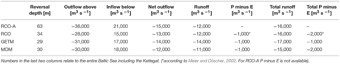
Table 2. Mean volume transports through Gotland transect calculated from the vertical profiles shown in Figure 9 for the ocean models RCO-A, RCO, GETM, and MOM as well as runoff and precipitation (P) minus evaporation (E) for this transect (numbers rounded to thousands).

Additionally, the 30-year mean depth-integrated volume transport per unit length for the Gotland transect is shown in Figure 10. For all models the transport is predominantly southward directed (negative) between Sweden and the western coast of Gotland. The magnitudes for RCO-A, RCO, and GETM are close to each other while MOM simulates a smaller transport. Between the eastern coast of Gotland and Latvia the structure of the gyre is visible with southward transport in the western part and northward transport in the eastern part. Here, the transports differ more for the individual models with strongest magnitudes simulated by GETM and smallest ones by MOM. The results of RCO-A and RCO are similar. Analogous 30-year mean depth-integrated volume transports per unit length for Arkona and Słupsk transects (not shown) reflect the patterns from Figure 8, which were described before.

FIGURE 10

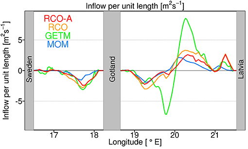
Figure 10. Depth-integrated flows per unit length orthogonal through Gotland transect as simulated by the ocean models RCO-A (red), RCO (orange), GETM (green), and MOM (blue) for the time period from 1970 to 1999.

Evaluation of Simulated Currents

The simulated currents were validated against ADCP measurements in the Arkona Basin (approximately in the center of the Arkona transect T1) and against mooring measurements near Gotland Deep (almost in the center of the eastern part of the Gotland transect T3; see Figure 1).

Arkona Basin

The statistics of the ADCP measurements are shown on the left-hand side of Figure 11 and were based on monthly averages of all datasets at a depth of 10 m below the surface. The 10-year mean observed zonal current velocity is close to 1.5 cm s⁻¹ and has a standard deviation of about ±9 cm s⁻¹. RCO-A, RCO, and MOM simulate a somewhat higher mean zonal current (about 3 cm s⁻¹) and a smaller standard deviation in the same order of magnitude as the mean. For GETM the zonal current at this location in the Arkona Basin varies around zero with a standard deviation of ±5 cm s⁻¹. The relative frequency of the observed and simulated zonal currents shows a good agreement between GETM and the ADCP measurements and clarifies also the similarity of RCO-A, RCO, and MOM with their higher means and smaller spread. Note, that some few ADCP outlier values between 62.5 and 67.5 cm s⁻¹ are not shown in the histogram.

FIGURE 11

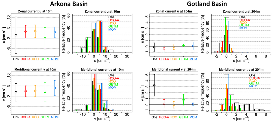
Figure 11. Mean current velocities with their standard deviations as well as relative frequency of these velocities from observations (black) and model simulations (colors) in the Arkona Basin at 10 m depth (left) and in the Gotland Basin at 204 m depth (right). Results for zonal components are shown in the top panels and for meridional components in the bottom panels. See text for further information.

The mean meridional current velocities observed and simulated at 10 m depth are more in accordance to each other. The ADCP measurements vary around a mean value of 2 cm s⁻¹ with a standard deviation of about ±4 cm s⁻¹. GETM lies very close to these values. MOM shows a similar variation as in the observations, but varies around a mean value of 4 cm s⁻¹. RCO-A and RCO have means of about 2.5 cm s⁻¹ with a standard deviation in the order of this mean. The respective relative frequencies reflect the relatively good agreement of the models with the measurements.

Gotland Basin

The statistics of the mooring observations near Gotland Deep shown on the right-hand side of Figure 11 are also based on monthly averages of all datasets, but at 204 m depth. The 5-year mean zonal current velocities and their standard deviations are very close to zero for both the mooring observations and the model simulations. The small deviation range is reflected by the relative frequency as well. Greater differences between measurements and models occur for the meridional current velocity. From the mooring observations it varies around a mean value of 3 cm s⁻¹ with a standard deviation of about ± 2 cm s⁻¹. In contrast, the models simulate again mean values around zero and standard deviations smaller than ±1 cm s⁻¹.

Evaluation of the Atmospheric Wind Data

Finally, the wind velocities of RCA3-ERA40 and coastDat2, which drive the ocean circulation models, were evaluated. The mean statistics over all stations along the Swedish coast which have been considered for this analysis are summarized in Table 3. They reveal partly substantial differences between observations and the forcing data. The mean zonal wind from both reanalysis datasets and the observations is directed eastward and is of the same magnitude. The mean meridional wind is directed northward, but the reanalysis datasets reproduce weaker magnitudes than in the observations. The strongest difference occurs for the mean wind speed, which is slightly overestimated by coastDat2 but largely underestimated by RCA3-ERA40. With some exceptions this also holds true for the individual stations. Also, root mean square differences (RMSDs), both for the wind components and for the wind speed, are larger in the RCA3-ERA40 than in the coastDat2 dataset.

TABLE 3

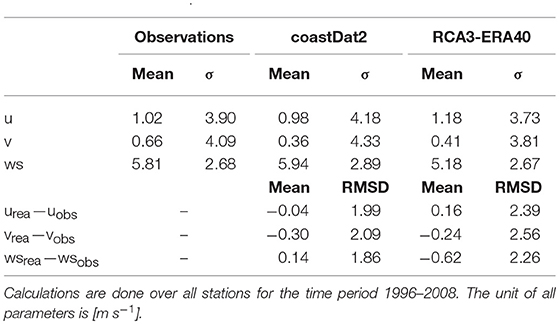
Table 3. Mean zonal wind speed (u), meridional wind speed (v), and total wind speed (ws) with their standard deviations (σ) for observations, coastDat2, and RCA3-ERA40 dataset as well as mean and root mean square difference (RMSD) between the reanalysis datasets (rea) and the observations (obs) for zonal, meridional, and total wind speed.

As an example the mean annual cycles of the wind speed at four stations along the Swedish coast are presented in Figure 12. At Skagsudde both reanalysis datasets agree well with the observations, but at the other three stations (Landsort, Ölands Norra Udde, and Måseskär) RCA3-ERA40 systematically underestimates the mean wind speed throughout the whole year. CoastDat2 is closer to the observations but also underestimates the mean wind speed at Landsort and Måseskär and overestimates it in autumn and winter at Ölands Norra Udde.

FIGURE 12

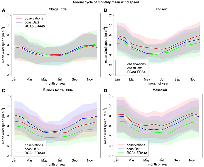
Figure 12. Annual cycle of monthly mean wind speed at selected stations around the Baltic Sea for the observations (red), coastDat2 (blue), and RCA3-ERA40 (green): (A) Skagsudde, (B) Landsort, (C) Ölands Norra Udde, and (D) Måseskär. The solid lines indicate the monthly mean and the shading indicates ±1 standard deviation.

Discussion

In this assessment the best results comparing observed and simulated temperature and salinity profiles are found for RCO-A. However, this finding is not surprising as the reanalysis temperature and salinity observations have been assimilated. The utilized observations are a sub-set of the BED database, that has been used in this study for the evaluation. Nevertheless, RCO simulations are very good even without data assimilation. Compared to models with level coordinates in vertical direction like RCO and MOM, GETM has the advantage of vertically adaptive coordinates, that minimizes spurious numerical mixing across isopycnals (diapycnical mixing) in the ocean interior (Gräwe et al., 2015). This reduced numerical mixing might cause the too shallow thermocline (Figure 2). The mixing in the surface well mixed layer is currently too low, which opens the possibility to see effects of additional parameterizations for surface waves effects and Langmuir-circulation. Although numerical mixing is still present in GETM, this mixing might mimic the effects of physical mixing, however, very likely for the wrong reason. Anyhow, this mixing in GETM corresponds better to recent observations than deep water mixing parameterizations used in level coordinate models (Holtermann and Umlauf, 2012; Holtermann et al., 2012, 2014, 2017).

Due to the assimilation of temperature and salinity measurements, we presume that in RCO-A the baroclinic part of the simulated current velocity fields is close to observations and can be used as a reference. However, the barotropic part, which is forced by the curl of the wind stress (calculated from wind velocity) minus the curl of the bottom drag, is not affected by the data assimilation and consequently not constrained by temperature and salinity observations.

In the following, selected hypotheses about the differences in both hydrography and circulation between the models are presented:

1. As all models reproduce temperature much better than salinity, it seems to be easier to calibrate the heat balance of Baltic Sea models than the water balance. However, in detail there are differences between the models. Largest mean biases in temperature are found in GETM perhaps because the parameterizations of the surface heat fluxes are not adopted to Baltic Sea conditions. Smallest biases and the most realistic mean seasonal cycle in temperature are found for RCO, which applies bulk formulae developed from flux measurements from the Baltic Sea region (Meier et al., 2003).

2. Although bottom salinities at Bornholm Deep and Gotland Deep are somewhat better reproduced in GETM than in RCO or MOM (with a more acceptable halocline depth in GETM and RCO than in MOM), in the Bothnian Sea and Bothnian Bay large biases were found in GETM. These problems might be caused by a different type of deep water formation process in the northern Baltic Sea (Bothnian Sea and Bothnian Bay) compared to the Baltic proper (Bornholm Basin and Gotland Basin). In the Baltic proper the deep water is renewed by saltwater intrusions from the North Sea, whereas in the Bothnian Sea and Bothnian Bay deep water might be formed by convection caused by cooling and brine release related to ice formation. Perhaps the present version of GETM with its thermodynamic sea ice model is not yet optimized for the latter process.

3. Mean surface velocities are much stronger in GETM than in the other models. A likely explanation is the zooming of the layers in GETM toward the surface. Here the minimum layer thickness can reach 50 cm, allowing a better representation of the wind shear effect in the surface layer. A further reason might be the larger wind speeds of the atmospheric forcing in GETM at least compared to RCO and RCO-A. Whether the stronger barotropic velocities in GETM are more realistic than in the other models cannot be decided as mentioned above. Since MOM is also driven by coastDat2 winds but simulates a weaker barotropic circulation than GETM, either the bottom drag or the horizontal viscosity together with the lateral drag (no-slip versus free-slip) in MOM is significantly larger than in GETM.

4. We identified several features of the currents differing among the models. For instance, the northward directed coastal current along the eastern Baltic Sea coast is more spatially centered and stronger in RCO and RCO-A than in GETM and MOM. Another detail is the stronger eastward flow through the Słupsk Channel in RCO and GETM than in MOM. Although in RCO-A the western sill of the Słupsk Channel was locally deepened, the results in that region do not differ much between RCO and RCO-A and the change in topography has no larger effect. Further, the barotropic circulation in Arkona Basin is stronger in RCO and RCO-A than in MOM and GETM perhaps because of the differing atmospheric forcing.

5. The vertical overturning or estuarine circulation is stronger in RCO-A than in MOM, GETM, or RCO perhaps because horizontal density gradients in RCO-A are larger than in the other models. The magnitude of the deep water ventilation is considerably affected by the use of data assimilation suggesting that internal pressure gradients still differ substantially among the models although at least GETM and RCO show acceptable agreement with observed temperature and salinity profiles at monitoring stations. Hence, a good agreement between model results and observed temperature and salinity profiles measured by Taylor diagrams and cost functions is only a necessary but not a sufficient condition for a realistically simulated thermohaline circulation. Note, that river runoff differs between the models (Table 2). For the halocline ventilation the results by RCO-A are close to the results from the diagnostic model by Elken (1996) (see also Meier, 2000, 2005; Meier and Kauker, 2003). Assuming geostrophically balanced currents, Elken (1996) calculated the mean flow east of Gotland between the transport minimum in 60 m depth and the sea bottom. An important question for future research is which data and quality measures are needed to evaluate the performance of climate models with respect to the estuarine overturning circulation properly.

6. The presented version of MOM performed worse in the Baltic proper compared to GETM or RCO/RCO-A. A possible reason might be that the calibration in MOM is less optimized. As both vertical (z-level) and horizontal (Arakawa B-grid) coordinates are similar in MOM and RCO there are no reasons to assume that MOM with the same forcing, model setup, sub-grid scale parameterizations and parameter settings will not perform at least as good as RCO. Earlier simulations suggest that differences due to the horizontal resolution between 1 and 3 nm are less important.

Summary, Conclusions, and Outlook

Summary

The present study deals with an assessment of the long-term mean circulation of the Baltic Sea as a classical example of a coastal sea as represented by various ocean circulation models, namely RCO (both in a conventional setup and an assimilation / reanalysis setup which is referred to RCO-A), GETM, and MOM. The capability of these models to represent physical conditions and processes of the Baltic Sea is investigated for a 30-year time period from 1970 through 1999. Simulations of temperature and salinity at monitoring stations are investigated by vertical profiles and statistical time series analysis at various depths taking Taylor diagrams and cost functions into account. As a reference dataset for comparisons post-processed observations of BED are used.

The main result is that observed temperature and salinity data are most realistically reproduced by the RCO-A reanalysis, which holds for temporal evolution, variability, and vertical profiles of these parameters. GETM and RCO show more deviations from the observations than RCO-A at certain monitoring stations and certain depths, but they still agree better with the BED data than MOM. In general, all models reproduce temperature well between the surface and 20 m depth. Salinity simulations are of predominantly good to reasonable quality for RCO and GETM independently of the depth except for stations which are located far north. The strongest deviations from observations occur for salinity simulated by MOM.

The investigation of the wind-driven circulation for the upper 10 m below the sea surface and of the depth-integrated volume transport for the entire Baltic Sea shows partly differing circulation patterns for the different models with GETM revealing strongest differences to RCO-A and greatest volume transports in the central Baltic Sea. The best agreement of currents and transport is found between RCO and RCO-A as expected.

Furthermore, mean current velocities and flows through three transects in the Arkona Basin, at the western entrance of Słupsk Channel, and in the Gotland Basin are examined. In general, all considered models show similar patterns at Arkona and Słupsk transect even though the location and magnitude of some circulation patterns varies. Smallest differences to RCO-A are found for RCO and strongest deviations occur for GETM. Numbers of near-surface outflows and inflows below the reversal depth disagree between RCO-A on the one hand and RCO, GETM, and MOM on the other hand.

The evaluation of simulated zonal and meridional current velocities from the used models with ADCP and mooring measurements at two monitoring stations shows an overall acceptable accordance. The model mean current velocities lie predominantly well within the standard deviation of the measurements except for the meridional current velocity near Gotland Deep. However, more observations from other depths are needed in order to allow a comprehensive evaluation.

The evaluation of the used atmospheric forcing datasets reveals that the mean wind speed is slightly overestimated by coastDat2, which drives the ocean circulation models GETM and MOM, but significantly underestimated by RCA3-ERA40, which is used for driving RCO-A and RCO.

Conclusions

The main conclusions of this study are:

1. Regardless of the chosen vertical coordinate system (z-level or vertically adaptive coordinates) and horizontal resolution (grid size between 1 and 3 nm) temperature and salinity observations at monitoring stations are reasonably reproduced by state-of-the-art regional ocean circulation models on a 30-year time scale provided that model setup and parameter calibration are correctly done.

2. Both the mean wind-driven and thermohaline circulation differ considerably between the models highlighting the need for additional long-term current measurements to assess the mean circulation in ocean models.

3. Model results with data assimilations provide the best available datasets to assess ocean models. However, data assimilation of temperature and salinity observations alone cannot constrain the mean currents. In addition to more current measurements, river runoff and wind velocity data need to be assessed more carefully because the datasets utilized in the various models differ considerably. These differences may explain some of the discovered differences in the ocean currents.

Outlook

These findings raise the question which model results represent the correct mean circulation of the entire Baltic Sea and its climate variability. To study the mean circulation and its variability further suitable long-term, high-frequency automated in situ observations for current velocity at additional stations are needed. Also, the potential location of new moorings will be calculated from model differences. In addition, the variability and sensitivity of the meridional overturning circulation to changes in atmospheric and hydrological forcing and saltwater inflows into the Baltic Sea will be investigated.

We propose to extend the Baltic Sea model assessment as an activity of the Baltic Earth program (Earth System Science for the Baltic Sea region, see http://www.baltic.earth) and invite other modeling groups to participate with their model results in the assessment following the methods and protocol of this study.

Data Availability Statement

Observations from the Baltic Environmental Database (BED) are publicly available from http://nest.su.se/bed. The raw data supporting the conclusions of this manuscript will be made available by the authors, without undue reservation, to any qualified researcher.

Author Contributions

MP and HEMM developed the concept of this study and worked predominantly on the manuscript. MP performed the main part of the data analysis and figure preparation. HEMM prepared the RCO model data and organized the corresponding database. UG prepared and provided the GETM data and contributed with ideas for the manuscript concept. TN processed and improved the MOM data during the analysis process. CF performed the comparison of the atmospheric wind data. YL prepared and provided the RCO-A reanalysis data. All authors contributed to manuscript revision, read and approved the submitted version.

Funding

YL was supported by the Swedish Research Council (VR) within the project Reconstruction and projecting Baltic Sea climate variability 1850-2100 (grant no. 2012-2117) and by the Swedish Research Council for Environment, Agricultural Sciences and Spatial Planning (FORMAS) within the project Cyanobacteria life cycles and nitrogen fixation in historical reconstructions and future climate scenarios (1850-2100) of the Baltic Sea (grant no. 214-2013-1449).

Conflict of Interest Statement

The authors declare that the research was conducted in the absence of any commercial or financial relationships that could be construed as a potential conflict of interest.

Acknowledgments

The research presented in this study is part of the Baltic Earth program. We thank the Federal Maritime and Hydrographic Agency Hamburg and Rostock (BSH) for financing and for supporting the operation of the MARNET stations in the western Baltic. We also thank our colleagues from the department of instrumentation at IOW for their relentless commitment before, during, and after monitoring ship cruises, and in particular Dr. Eberhard Hagen, Günter Plüschke, and Toralf Heene for providing the measurement data. Further, we acknowledge the support of the IOW IT department for managing the archive of long-term measurement data (see http://iowmeta.io-warnemuende.de). Temperature and salinity data used for evaluation are open access and were extracted from the Baltic Environmental Database (BED, http://nest.su.se/bed) at Stockholm University and all data providing institutes (listed at http://nest.su.se/bed/ACKNOWLE.shtml) are kindly acknowledged. The model development and simulations for GETM and MOM were performed with resources provided by the North-German Supercomputing Alliance (HLRN). We thank Uwe Schulzweida, the R Core Team, and the Unidata development team (and all involved developers/contributors) for maintaining the open source software packages Climate Data Operators (cdo), the statistical computing language R, and netCDF, respectively.

References

Andrejev, O., Myrberg, K., Alenius, P., and Lundberg, P. A. (2004a). Mean circulation and water exchange in the Gulf of Finland–a study based upon three-dimensional modeling. Boreal Environ. Res. 9, 1–16.

Google Scholar

Andrejev, O., Myrberg, K., and Lundberg, P. A. (2004b). Age and renewal time of water masses in a semi-enclosed basin–application to the Gulf of Finland. Tellus A 56, 548–558. doi: 10.3402/tellusa.v56i5.14435

CrossRef Full Text | Google Scholar

Bergström, S., and Carlsson, B. (1994). River runoff to the Baltic Sea−1950-1990. Ambio 23, 280–287.

Google Scholar

Burchard, H., and Bolding, K. (2002). GETM–A General Estuarine Transport Model: Scientific Documentation. Technical Report EUR 20253 EN, European Commission.

Dee, D. P., Uppala, S. M., Simmons, A. J., Berrisford, P., Poli, P., Kobayashi, S., et al. (2011). The ERA-Interim reanalysis: configuration and performance of the data assimilation system. Q. J. R. Meteorol. Soc. 137, 553–597. doi: 10.1002/qj.828

CrossRef Full Text | Google Scholar

Deleersnijder, E., Campin, J.-M., and Delhez, E. J. M. (2001). The concept of age in marine modeling: I. Theory and preliminary model results. J. Marine Syst. 28, 229–267. doi: 10.1016/S0924-7963(01)00026-4

CrossRef Full Text | Google Scholar

Döös, K., Meier, H. E. M., and Döscher, R. (2004). The Baltic haline conveyer belt or the overturning circulation and mixing in the Baltic. AMBIO 33, 261–266. doi: 10.1579/0044-7447-33.4.261

PubMed Abstract | CrossRef Full Text | Google Scholar

Eilola, K., Gustafsson, B. G., Kuznetsov, I., Meier, H. E. M., Neumann, T., and Savchuk, O. P. (2011). Evaluation of biogeochemical cycles in an ensemble of three state-of-the-art numerical models of the Baltic Sea. J. Marine Syst. 88, 267–284. doi: 10.1016/j.jmarsys.2011.05.004

CrossRef Full Text | Google Scholar

Elken, J. (1996). Deep Water Overflow, Circulation and Vertical Exchange in the Baltic Proper. Report Series No.6 (Tallinn: Estonian Marine Institute), 91.

Elken, J., and Matthäus, W. (2008). “Baltic Sea oceanography,” in BALTEX Assessment of Climate Change for the Baltic Sea Basin (BACC), ed H. von Storch (Berlin: Springer), 379–386.

Geyer, B. (2014). High-resolution atmospheric reconstruction for Europe 1948-2012: coastDat2. Earth Syst. Sci. Data 6, 147–164. doi: 10.5194/essd-6-147-2014

CrossRef Full Text | Google Scholar

Gräwe, U., Flöser, G., Gerkema, T., Duran-Matute, M., Badewien, T. H., Schulz, E., et al. (2016). A numerical model for the entire Wadden Sea: skill assessment and analysis of hydrodynamics. J. Geophys. Res. Oceans 121, 5231–5251. doi: 10.1002/2016JC011655

CrossRef Full Text | Google Scholar

Gräwe, U., Holtermann, P., Klingbeil, K., and Burchard, H. (2015). Advantages of vertically adaptive coordinates in numerical models of stratified shelf seas. Ocean Model. 92, 56–68. doi: 10.1016/j.ocemod.2015.05.008

CrossRef Full Text | Google Scholar

Griffies, S. M. (2004). Fundamentals of Ocean Climate Models. Princeton, NJ: Princeton University Press.

Google Scholar

Gustafsson, B. G., and Rodriguez-Medina, M. (2011). Validation data set compiled from Baltic Environmental Database, (Version 2, January 2011). Baltic Nest Institute Technical Report No.2, (Stockholm).

Hagen, E., and Feistel, R. (2004). Observations of low-frequency current fluctuations in deep water of the Eastern Gotland Basin/Baltic Sea. J. Geophys. Res. 109:C03044. doi: 10.1029/2003JC002017

CrossRef Full Text | Google Scholar

HELCOM (2015). “Updated fifth Baltic Sea pollution load compilation (PLC-5.5),” in Baltic Sea Environment Proceedings No. 145, 1–142.

Hofmeister, R., Burchard, H., and Beckers, J.-M. (2010). Non-uniform adaptive vertical grids for 3D numerical ocean models. Ocean Model. 33, 70–86. doi: 10.1016/j.ocemod.2009.12.003

CrossRef Full Text | Google Scholar

Höglund, A., Meier, H. E. M., Broman, B., and Kriez, E. (2009). Validation and Correction of Regionalised ERA-40 Wind Fields Over the Baltic Sea using the Rossby Centre Atmosphere Model RCA3.0. Rapport Oceanografi No. 97. Norrköping: SMHI.

Google Scholar

Holtermann, P. L., Burchard, H., Gräwe, U., Klingbeil, K., and Umlauf, L. (2014). Deep-water dynamics and boundary mixing in a nontidal stratified basin: a modeling study of the Baltic Sea. J. Geophys. Res. Oceans 119, 1465–1487. doi: 10.1002/2013JC009483

CrossRef Full Text | Google Scholar

Holtermann, P. L., Prien, R., Naumann, M., Mohrholz, V., and Umlauf, L. (2017). Deepwater dynamics and mixing processes during a major inflow event in the central Baltic Sea. J. Geophys. Res. Oceans 122, 6648-6667. doi: 10.1002/2017JC013050

CrossRef Full Text | Google Scholar

Holtermann, P. L., and Umlauf, L. (2012). The Baltic sea tracer release experiment: 2. mixing processes. J. Geophys. Res. 117:C01022. doi: 10.1029/2011JC007445

CrossRef Full Text | Google Scholar

Holtermann, P. L., Umlauf, L., Tanhua, T., Schmale, O., Rehder, G., and Waniek, J. J. (2012). The Baltic sea tracer release experiment: 1. mixing rates. J. Geophys. Res. 117:C01021. doi: 10.1029/2011JC007439

CrossRef Full Text | Google Scholar

Kalnay, E., Kanamitsu, M., Kistler, R., Collins, W., Deaven, D., Gandin, L., et al. (1996). The NCEP/NCAR 40-year reanalysis project. Bull. Am. Meteorol. Soc. 77, 437–471. doi: 10.1175/1520-0477(1996)077<0437:TNYRP>2.0.CO;2

CrossRef Full Text | Google Scholar

Killworth, P. D., Stainforth, D., Webb, D. J., and Paterson, S. M. (1991). The development of a free-surface Bryan-Cox-Semtner ocean model. J. Phys. Oceanogr. 21, 1333–1348. doi: 10.1175/1520-0485(1991)021<1333:TDOAFS>2.0.CO;2

CrossRef Full Text | Google Scholar

Krüger, S. (2000). “Basic shipboard instrumentation and fixed automatic stations for monitoring in the Baltic Sea,” in The Ocean Engineering Handbook, ed El-Hawary (Boca Raton, FL: CRC Press LLC, N. W. Corporate Blvd), 52.

Google Scholar

Large, W. G., McWilliams, J. C., and Doney, S. C. (1994). Oceanic vertical mixing: a review and a model with a nonlocal boundary layer parameterization. Rev. Geophys. 32, 363–403. doi: 10.1029/94RG01872

CrossRef Full Text | Google Scholar

Lehmann, A., and Hinrichsen, H.-H. (2000). On the wind driven and thermohaline circulation of the Baltic Sea. Phys. Chem. Earth 25, 183–189. doi: 10.1016/S1464-1909(99)00140-9

CrossRef Full Text | Google Scholar

Liu, Y., Meier, H. E. M., and Axell, L. (2013). Reanalyzing temperature and salinity on decadal time scales using the ensemble optimal interpolation data assimilation method and a 3-D ocean circulation model of the Baltic Sea. J. Geophys. Res. Oceans 118, 5536–5554. doi: 10.1002/jgrc.20384

CrossRef Full Text | Google Scholar

Liu, Y., Meier, H. E. M., and Eilola, K. (2014). Improving the multiannual, high-resolution modelling of biogeochemical cycles in the Baltic Sea by using data assimilation. Tellus A 66:1. doi: 10.3402/tellusa.v66.24908

CrossRef Full Text | Google Scholar

Liu, Y., Meier, H. E. M., and Eilola, K. (2017). Nutrient transports in the Baltic Sea–results from a 30-year physical-biogeochemical reanalysis. Biogeosciences 14, 2113–2131.doi: 10.5194/bg-14-2113-2017

CrossRef Full Text | Google Scholar

Löptien, U., and Meier, H. E. M. (2011). The influence of increasing water turbidity on the sea surface temperature in the Baltic Sea: a model sensitivity study. J. Marine Syst. 88, 323–331. doi: 10.1016/j.jmarsys.2011.06.001

CrossRef Full Text | Google Scholar

Matthäus, W., and Franck, H. (1992). Characteristics of major Baltic inflows–a statistical analysis. Cont. Shelf Res. 12, 1375–1400. doi: 10.1016/0278-4343(92)90060-W

CrossRef Full Text | Google Scholar

Meier, H. E. M. (2000). The Use of the κ-ε Turbulence Model within the Rossby Centre Regional Ocean Climate Model: Parameterization Development and Results. Reports Oceanography No. 28, Norrköping: SMHI, 81.

Meier, H. E. M. (2001). On the parameterization of mixing in three-dimensional Baltic Sea models. J. Geophys. Res. 106, 30997–31016. doi: 10.1029/2000JC000631

CrossRef Full Text | Google Scholar

Meier, H. E. M. (2005). Modeling the age of Baltic Sea water masses: quantification and steady state sensitivity experiments. J. Geophys. Res. 110:C02006. doi: 10.1029/2004JC002607

CrossRef Full Text | Google Scholar

Meier, H. E. M. (2007). Modeling the pathways and ages of inflowing salt- and freshwater in the Baltic Sea. Estuar. Coast. Shelf Sci. 74, 610–627. doi: 10.1016/j.ecss.2007.05.019

CrossRef Full Text | Google Scholar

Meier, H. E. M., and Döscher, R. (2002). Simulated water and heat cycles of the Baltic Sea using a 3D coupled atmosphere-ice-ocean model. Boreal Env. Res. 7, 327–334.

Google Scholar

Meier, H. E. M., Döscher, R., and Faxén, T. (2003). A multiprocessor coupled ice-ocean model for the Baltic Sea: application to salt inflow. J. Geophys. Res. 108:3273. doi: 10.1029/2000JC000521

CrossRef Full Text | Google Scholar

Meier, H. E. M., Höglund, A., Döscher, R., Andersson, H., Löptien, U., and Kjellström, E. (2011). Quality assessment of atmospheric surface fields over the Baltic Sea from an ensemble of regional climate model simulations with respect to ocean dynamics. Oceanologia 53, 193–227. doi: 10.5697/oc.53-1-TI.193

CrossRef Full Text | Google Scholar

Meier, H. E. M., and Kauker, F. (2003). Modeling decadal variability of the Baltic Sea: 2. Role of freshwater inflow and large-scale atmospheric circulation for salinity. J. Geophys. Res. 108:3368.doi: 10.1029/2003JC001799

CrossRef Full Text | Google Scholar

Myrberg, K., and Andrejev, O. (2006). Modelling of the circulation, water exchange and water age properties of the Gulf of Bothnia. Oceanologia 48, 55–74.

Google Scholar

Myrberg, K., Ryabchenko, V., Isaev, A., Vankevich, R., Andrejev, O., Bendtsen, J., et al. (2010). Validation of three-dimensional hydrodynamic models of the Gulf of Finland. Boreal Environ. Res. 15, 453–479.

Google Scholar

Neumann, T., Fennel, W., and Kremp, C. (2002). Experimental simulations with an ecosystem model of the Baltic Sea: A nutrient load reduction experiment. Global Biogeochem. Cycles 16, 7-1–7-19. doi: 10.1029/2001GB001450

CrossRef Full Text | Google Scholar

Neumann, T., Radtke, H., and Seifert, T. (2017). On the importance of Major Baltic Inflows for oxygenation of the central Baltic Sea. J. Geophys. Res. Oceans 122, 1090–1101. doi: 10.1002/2016JC012525

CrossRef Full Text | Google Scholar

Omstedt, A., and Nohr, C. (2004). Calculating the water and heat balances of the Baltic Sea using ocean modelling and available meteorological, hydrological and ocean data. Tellus A 56, 400–414. doi: 10.3402/tellusa.v56i4.14428

CrossRef Full Text | Google Scholar

Pacanowski, R. C., and Griffies, S. M. (2000). MOM 3.0 Manual. Technical Report, Geophysical Fluid Dynamics Laboratory.

Google Scholar

Pätsch, J., Burchard, H., Dieterich, C., Gräwe, U., Gröger, M., Mathis, M., et al. (2017). An evaluation of the North Sea circulation in global and regional models relevant for ecosystem simulations. Ocean Model. 116, 70–95. doi: 10.1016/j.ocemod.2017.06.005

CrossRef Full Text | Google Scholar

Samuelsson, P., Jones, C. G., Willén, U., Ullerstig, A., Gollvik, S., Hansson, U., et al. (2011). The Rossby Centre Regional Climate model RCA3: model description and performance. Tellus A 63, 4–23. doi: 10.1111/j.1600-0870.2010.00478.x

CrossRef Full Text | Google Scholar

Sarkisyan, A. S., Staskwiecz, A., and Koalik, Z. (1975). Diagnostic computation of the summer circulation in the Baltic Sea. Oceanologia 15, 653–656.

Smagorinsky, J. (1963). General circulation experiments with the primitive equations: 1. The basic experiment. Monthly Weather Rev. 91, 99–164. doi: 10.1175/1520-0493(1963)091<0099:GCEWTP>2.3.CO;2

CrossRef Full Text | Google Scholar

Stigebrandt, A. (1987). Computations of the flow of dense water into the Baltic Sea from hydrographical measurements in the Arkona Basin. Tellus A 39A, 170–177.

Google Scholar

Taylor, K. E. (2001). Summarizing multiple aspects of model performance in a single diagram. J. Geophys. Res. 106, 7183–7192. doi: 10.1029/2000JD900719

CrossRef Full Text | Google Scholar

Uppala, S. M., KÅllberg, P. W., Simmons, A. J., Andrae, U., Bechtold, V. D. C., Fiorino, M., et al. (2005). The ERA-40 re-analysis. Q. J. R. Meteorol. Soc. 131, 2961–3012. doi: 10.1256/qj.04.176

CrossRef Full Text | Google Scholar