Influence of Surfactant Concentration and Temperature Gradients on Spreading of Crude-Oil at Sea*

Introduction

The kinetics of spreading various liquid hydrocarbons (including crude oil and petroleum substances) on the surface of the original seawater were investigated using video-microscopy and dynamic tensometry under laboratory conditions. The aqueous phase, containing natural surfactants, formed on the surface an adsorption layer with specific viscoelastic properties, which were determined by means of supplementary measurements with the Langmuir technique (Boniewicz-Szmyt and Pogorzelski, 2016). The classic spreading theory, so-called laminar flow theory of the boundary layer (Camp and Berg, 1987; Craster and Matar, 2006) is applicable to the system of immiscible, insoluble, and chemically pure liquids and predicts the rate of expansion of the oil spot 6–9 times higher than that was observed in previous studies (Boniewicz-Szmyt and Pogorzelski, 2008). The form of the dependence: oil lens radius vs. time r_L ~ K tⁿ, shows the power-law character. However, the exponent n proved to be close to ¾ for non-volatile substances but was lower oscillating around ½ for volatile hydrocarbons (Dussaud and Troian, 1998). The K constant is a function of the viscoelasticity of water phase (in particular, the dilational elasticity modulus E_AW). The change in the exponent n, from the initial value ¾ to ½, appeared as an inflection point in the dependence r_L(t) for volatile substances, occurred after a certain time t (of the order seconds), from the moment of oil substance deposition, which pointed to the activation of the additional underestimated fluid flow mechanism. As a first step made to eliminate the discrepancy between the experimentally measured and theoretically predicted oil on water spreading velocity, the existing model was corrected by replacing the static spreading coefficient S₀ with the dynamic one S_t (Boniewicz-Szmyt and Pogorzelski, 2008). That explained only the observed stopping of the expansion of oil lens edge when S_t attained 0, and revealed the dependence r_L(E_AW).

The aim of the work is to determine the effect of surface tension gradients induced by inhomogeneities in the distribution of natural seawater surfactant concentrations, and temperature gradients in the upper surface micro-layer on the flow of fluids in the course of oil substance spreading process. The Benard-Marangoni circulation in the near-surface region results from the so-called Marangoni effect (Chauvet et al., 2012). Surface tension gradients cause Benard-Marangoni instability and creation the extremely dissipative, turbulent of cell-like fluid flow, in thin layers (several millimeters) of volatile petroleum products, during the spreading process, in the final stage of the process, where surface tension forces play a main role surface (Perfetti and Iorio, 2014). It was assumed that the evaporation process of volatile hydrocarbons with a sufficiently high evaporation rate E (gs⁻¹), can initiate the appearance of circulation cells in the expanding oil layer if the threshold temperature difference ΔT_c (between the lower and upper surface of the expanding lens layer) is attained. It appears for the so-called Marangoni number exceeding the critical value (Chauvet et al., 2012). The required ΔT was determined for model hydrocarbons on the basis of their physico-thermal properties and thermo-elastic surface parameters of the original seawater (Boniewicz-Szmyt and Pogorzelski, 2016). The directly performed the evaporative hydrocarbon surface cooling measurements (using a thermal infrared sensor) allowed us to conclude that ΔT ~ E and the induced temperature gradients are sufficiently high to initiate the Benard-Marangoni dissipative flow accompanying the oil substance spreading at seawater.

Even though the classical spreading equations developed by Fay form the basis for the most spreading algorithms in use in oceanographic practice, it is well-established that oil spreading cannot be fully explained by these relations (Fingas, 2012, 2013). As a consequence, many of the formalisms used in crude oil spill models are often quite simple and attempt to describe only the gross evolution of the oil slick, ignoring finer scale processes.

Surface Tension-Driven Spreading—Theory and Problem Formulation

Earlier spreading dynamics studies of non-volatile, insoluble thin oil layers on a thick liquid layer showed that the leading edge of the expanding lens moves with time like t^3/4, according to the laminar theory of the boundary layer (Camp and Berg, 1987; Craster and Matar, 2006). However, we have evidenced that the leading edge of volatile, immiscible spreading films also advances as a power law in time i.e., tⁿ but with n ~ 1/2 (Boniewicz-Szmyt and Pogorzelski, 2008) in the form:

$\begin{array}{ll}{r}_L(t)=K\left[\frac{{S_0}^{1/2}}{{(\mu \rho )}^{1/4}}\right]t^n,& (1)\end{array}$

where μ and ρ are the viscosity and density of the substrate liquid, respectively, and K is an experimental constant dependent on the dilational viscoelasticity E_AW of the sea water surface (Figure 7 in Boniewicz-Szmyt and Pogorzelski, 2008).

Whether or not oil or surface active material will spread depends on the sign of the spreading coefficient S₀ (Boniewicz-Szmyt et al., 2007). Its positive value means a spontaneous process (Adamson and Gast, 1997):

$\begin{array}{ll}{S}_0={\gamma }_{AW}-{\gamma }_{OA}-{\gamma }_{OW},& (2)\end{array}$

where γ_AW is the surface tension of the air/water interface, γ_OA is the surface tension of air/oil interface, and γ_OW is the interfacial tension of water/oil interface. Spreading liquid films and water subphase can contain surface active materials like: detergents, fatty acids, phospholipids, and resins and asphaltens (in crude oil, Bauget et al., 2001). Any deformation of an elastic film-covered (of elasticity modulus E_AW) water surface either by shear or dilational compression will be resisted by the corresponding surface tension change:

$\begin{array}{ll}\Delta {\gamma }_f=E_{AW}\left(\frac{\Delta A}{A}\right),& (3)\end{array}$

where ΔA/A is the relative film area change.

As a result, if surface active material is already present at the air/water interface, the rate of spreading dr_L/dt and the area over which the oil spreads are reduced. The compression of the initial layer of surface active material resulting from oil drop spreading leads to a further time-dependent decrease of S₀. The initial spreading coefficient S₀ in Equation (1) should be corrected, and takes the form (Boniewicz-Szmyt and Pogorzelski, 2008):

$\begin{array}{ll}{S}_t=S_0-\Delta {\gamma }_f,& (4)\end{array}$

where S_t is the temporal spreading coefficient.

Solutal and Thermal Marangoni Effect

Spontaneous flow toward regions of high surface tension, so-called Marangoni flow, is a very fast transport process whose speed is mediated by the surface tension gradients (Pearson, 1958). Temperature gradients ΔT and differences in concentration of Δc surfactants (thermal and classic Marangoni effect) lead to tangential interfacial stresses and development of circulating cells (Chauvet et al., 2012).

The direction of fluid circulation in the liquid layer, with the horizontal ΔT_|| and the vertical temperature gradient △T_⊥ (Unny and Niessen, 1969), along with the concentration gradients of surface active substances (Li and Mao, 2001), is shown in Figure 1.

FIGURE 1

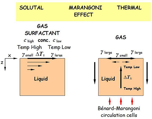
Figure 1. Mechanism of surface tension-driven flow (modified after Hibiya and Ozawa, 2013).

Under equilibrium conditions, shear stresses induced by surface tension gradients are balanced by viscous stresses, which leads, in two dimensions: x-horizontal and z-vertical coordinates, to the Equation (Mao et al., 2008):

$\begin{array}{ll}\mu \frac{\partial U_s}{\partial z}=-\frac{\partial \gamma }{\partial T}·\frac{\partial T}{\partial x}-\frac{\partial \gamma }{\partial c}·\frac{\partial c}{\partial x},& (5)\end{array}$

where U_s is the velocity of surface flow (m s⁻¹), μ the dynamic viscosity (Pa s), ∂γ/∂T = γ_T the surface entropy (mN m⁻¹ K⁻¹), ∂γ/∂c = γ_c the surfactant activity (mN m²mol⁻¹).

The current surface tension of γ liquid, in the presence of non-uniform spatial distribution of the surface active substance concentration (c – c₀), and temperature differences (T – T₀) is described by the relationship:

$\begin{array}{ll}\gamma ={\gamma }_0\left[1-{\gamma }_T(T-T_0)-{\gamma }_c(c-c_0)\right].& (6)\end{array}$

The final effect of the Marangoni mechanism depends on the physico-thermal properties of the liquid as well as on the surface activity of a surfactant.

The linear velocity U_s of the outermost surface regions, under the temperature gradient perpendicular to the mean spreading flow direction, in circulation cells, for a layer of thickness d of the liquid describes the relationship (Berg, 2009):

$\begin{array}{ll}{U}_s=\frac{1}{4}\frac{\frac{\partial \gamma }{\partial T}\frac{\partial T}{\partial x}d}{\mu }.& (7)\end{array}$

For d (~ milimeters), U_s = 0.1–0.3 cms⁻¹.

In order to form the Benard-Marangoni convection cell, the system must exceed the critical Rayleigh or Marangoni numbers (i.e., any one of them) both of which are proportional to the vertical temperature differences, and are defined in the form (Toussaint et al., 2008):

$\begin{array}{l}\text{Number Marangoni Number Rayleigh}\\ Ma=\frac{\partial \gamma }{\partial T}·\frac{\Delta Td}{\rho \nu \kappa },Ra=\frac{\alpha g\Delta T{d}^3}{\nu \kappa },& (8)\end{array}$

where γ is the surface tension (mN m⁻¹), ΔT the temperature difference (K), ρ the liquid density (kgm⁻³), ν the kinematic viscosity (m²s⁻¹), κ the thermal diffusivity (m²s⁻¹), d the fluid layer thickness (m), α the thermal volume expansion coefficient (K⁻¹), g is acceleration due to gravity (ms⁻²).

The following critical values of the numbers are usually reported for the formation of circulation cells: Ma_c = 81; Ra_c = 680 (Toussaint et al., 2008).

Since the numbers: Ma ~ d and Ra ~ d³, the critical temperature differences (from Equation 8) are related to d as: (ΔT_crit)_Ma ~ d⁻¹ and (ΔT_crit)_Ra ~ d⁻³. For thin layers (d of the order of millimeters), the temperatures remain to each other in the following relationship (ΔT_crit)_Ma << (ΔT_crit)_Ra, which means that the Marangoni mechanism associated with surface tension gradients requires much lower temperature to activate than the Rayleigh mechanism attributed to the convective movements caused by vertical liquid density differences (Sefiane and Ward, 2007). Even small temperature differences (of 0.3 K), easily achieved in spreading of volatile hydrocarbons, are capable of creating the circulation cells (Toussaint et al., 2008). Critical temperatures ΔT_c have been estimated on the physical and thermal properties of the model substances and subsequently compared with those measured in the evaporation rate experiment. In order to evaluate the threshold ΔT_c required to initiate the B-M circulation, for a non-volatile model liquid a separate experiment was performed.

It is worth noting that with the increase of ΔT, the flow of liquid in B-M cells, initially stable and regular, takes on the oscillatory character, until it finally becomes completely turbulent, as illustrated in Figure 2 (Yoda, 2007).

FIGURE 2

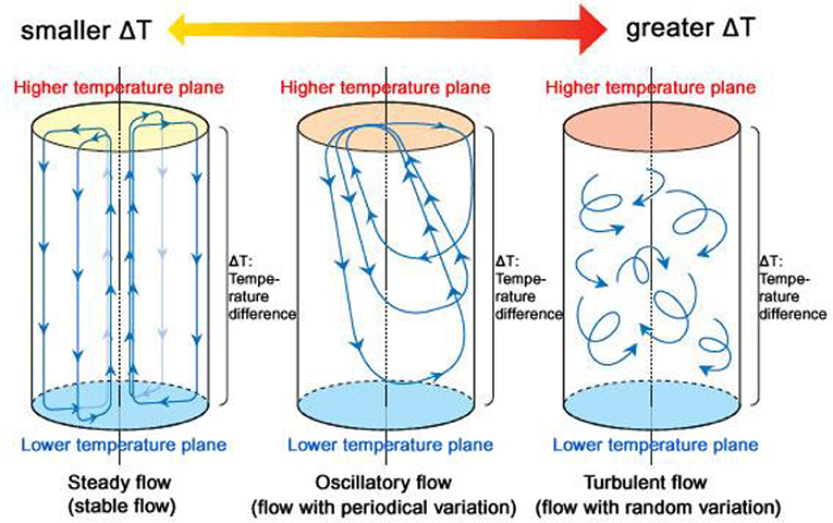
Figure 2. The temperature effect on B-M flow pattern. The initial steady flow turns into a flow with periodical variations called an oscillatory flow, and then the flow becomes completely disordered named a turbulent flow with an increase of temperature difference ΔT (Yoda, 2007).

Materials and Methods

Research Material

In oil substance spreading dynamics studies on the water phase, four types of crude oil were used (Romashkino, Flotta, Petrobaltic, Podkarpacka), and pure hydrocarbons of differentiated volatility (silicon oil, ethanol and acetone) as model substances deposited at the sea water collected in coastal waters (Gulf of Gdansk, Baltic Sea). Physical and thermal parameters of the studied hydrocarbons were obtained from table reference data (Bejan, 2004; Riazi, 2005; Jones, 2010), while the thermo-elastic properties of air/water (A/W) and air/oil (A/O) interfaces have been determined in our previous studies (Boniewicz-Szmyt and Pogorzelski, 2016). They were used as input data for the theoretical estimation of the threshold value ΔT_c.

Kinetics Measurements of Oil Spreading on Water

Spreading dynamics of model of hydrocarbons on the surface of original sea water samples were performed in a thermostated measuring tank using the video cameras, computer-aided image recording system, as described in detail together with the conditions of experiment methodology in Boniewicz-Szmyt and Pogorzelski (2008).

B-M Circulation Imaging, Temperature Distribution, and Evaporation Rate Measurements

The scheme of the experimental set-up used for non-contact, continuous recording and spatial mapping of the temperature difference ΔT between the free surface of the liquid and the base of the layer, using the IR sensor camera, is shown in Figure 3 (adapted after Pasquetti et al., 2002).

FIGURE 3

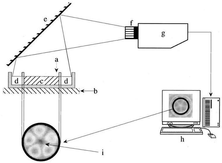
Figure 3. Diagram of experimental set-up for B-M cellular flow studies: a—free surface of test liquid, b—heated plate with temperature controller, resting on analytical electro balance, c—probe liquid in Peltier dish, d—container, e—inclined aluminum mirror, f—long-focus lens, g—IR camera (infrared light range, 3–5 μm sensor wavelength, ΔT ~ 20 mK resolution), h—computer with data acquisition and image analysis, i—exemplary image of liquid surface with cellular temperature spatial distribution (modified after Pasquetti et al., 2002).

In the first stage of the experiment, the non-volatile liquid layer (silicone oil) was heated from below using a heating bottom mat in order to introduce a controlled vertical temperature gradient (ΔT ~ 2 K for a liquid thickness d = 2.4 mm), recording the development of the circulation cells.

In the case of volatile substances, the differential temperature ΔT was measured simultaneously during the evaporation process and the weight sample decrease as a function of time was recorded with an electro balance to calculate the evaporation rate E = (dm/dt). The images were graphically analyzed (ImageJ program) to determine the specific cell flow features and the spatial distribution of the sample surface temperature.

Results and Discussion

Spreading of Oil Substances Over Sea Water

The spreading kinetics of different crude oils and their derivatives were already presented and discussed in detail elsewhere (Boniewicz-Szmyt and Pogorzelski, 2008). The r_L-time dependences, discussed here as an example, can be found in Figures 4, 6 in Boniewicz-Szmyt and Pogorzelski (2008), for crude oil products where the “switch over” time, marked with the arrow, was ranging from t = 0.5–20 s clearly dependent on the substance volatility. The similar r_L = 4.86 t^0.49 relation was found by Dussaud and Troian (1998), for toluene.

FIGURE 4

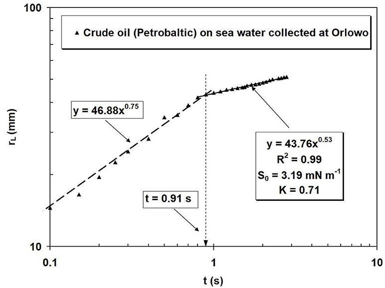
Figure 4. Radius r_L vs. time for 1 mm³m volume crude oil (Petrobaltic) drop on sea water collected at Orlowo (Gulf of Gdansk, Baltic Sea). The solid line (–) corresponds to the time dependence with n = 3/4, whereas the dashed (- - - -) one results from the best-fit least-squares approximation applied to the experimental data. A vertical line points to the “switch over” time, at which the transition from “nonvolatile” to “volatile” spreading regime starts.

An exemplary radius time history r_L(t), for 1-mm³m drops crude oil (Petrobaltic) spreading on sea water collected in Orlowo is depicted in Figure 4 on logarithmic scales, which is characteristic for all the tested volatile liquids.

In the initial part (short times), the dependence follows the power-law function (Equation 1) with the exponent n = 3/4, applicable to non-volatile liquids. As the evaporation process progresses, after time t = 0.91 s, the exponent n becomes closer to ½, characteristic for volatile liquids (Toussaint et al., 2008). The observed effect can result from the initiation of a specific flow analogous to the B-M circulation caused by surface cooling as a result of intensive evaporation of the volatile substance. Moreover, differences in the liquid vapor pressure or the spreading coefficient seem only to affect the speed of advance but not the value of spreading exponent (Dussaud and Troian, 1998). There is an evidence of an particular thermal boundary layer created in the base liquid. This thermal layer corresponds to the development of a vertical temperature gradient induced in the liquid support during the rapid spreading and evaporation process. The observed decrease of the spreading exponent found in volatile films can be attributed to the presence of a Benard-Marangoni type convective roll which develops beneath the leading edge. This strong circulation pattern may be the additional source of dissipation required to diminish the spreading exponent (Dussaud and Troian, 1998).

In the experiments, using a reflected laser beam for visualization of the flow, during the spreading process a thin layer of the volatile liquid (toluene), the picture of this phenomenon was evidenced (Figure 5).

FIGURE 5

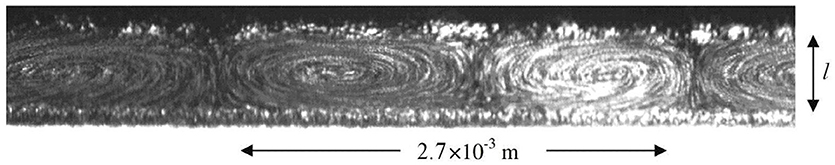
Figure 5. Toluene spreading experiment visualized with aluminum dust particles and laser scattering technique, layer thickness l = 0.8 mm. B-M cells dimension ~ 3.3 × l (Toussaint et al., 2008).

This allows to propose the model of spreading a thin layer of insoluble but volatile oil substance on the water phase in the form illustrated in Figure 6.

FIGURE 6

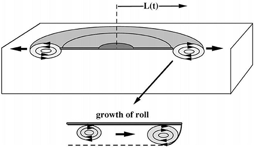
Figure 6. Sub-surface flow in the water phase observed during volatile oil film spreading. Below a magnified view of stretched roll which produces flat thermal layer therein (Dussaud and Troian, 1998).

This kind of fluid circulation is caused by evaporation and the accompanied process of surface cooling, during the rapid spreading of the film, resembles B-M circulation flow. This leads to the induction of an additional mechanism of fluid flow energy dissipation and subsequently to slow down the spreading process, as evidenced previously in Boniewicz-Szmyt and Pogorzelski (2008).

The standard Fay oil spill spreading model at sea divides the process into three stages: the gravity-inertial phase, gravity viscous phase, and viscous-surface tension phase (Lehr and Simecek-Beatty, 2000). It appears that it is difficult to construct a spreading formula applicable in all circumstances, while the Fay formulas may be theoretically sound, they have performed poorly in experimental and actual spills. For example, the extend of spread R(t) was proposed to obey the power law with respect to time: R(t) = m tⁿ, where m is the pre-exponential constant (Njobuenwu and Abowei, 2008). For an elongated ellipse along the wind direction oil spill shape, the non-symmetrical spreading was found, and in the case of minor and major axes relations r_L ~ t^0.5 and r_L ~ t^1.0, respectively were reported (Giwa and Jimoh, 2010). However, if the spreading was caused by a first stage shear diffusion process then the elongation would be proportional to t^1.5, while a second stage process would cause it to grow as t^0.5. The numerical results suggest that the observed spreading is a mixture of the two processes (Elliott, 1986). The realistic model of oil spreading should include the shear diffusion that is associated with vertical shears resulting also from small-scale processes like Benard-Marangoni phenomenon.

B-M Circulation vs. Thermo-Physical Properties of Hydrocarbons

The B-M circulation experiments presented here, for a non-volatile model liquid, were necessary to evaluated the threshold ΔT_c, which turned out to be much higher (a few K) than evaluated for the volatile liquids. That explains the result of the our previous kinetics studies performed also for crude oil products (non-volatile), where the “swith over” time was not observed as attributed to the transition from r_L ~ t^¾ to t^0.5 (Boniewicz-Szmyt and Pogorzelski, 2008).

A thermo-graphic image of the non-volatile liquid layer surface (silicone oil with a layer thickness d = 2.1 mm, placed in a cylinder vessel with an inner diameter D = 7.4 cm, bottom heated by a regulated electric device) observed for the surface-bottom temperature difference ΔT = 2.5 K, is shown in Figure 7A.

FIGURE 7

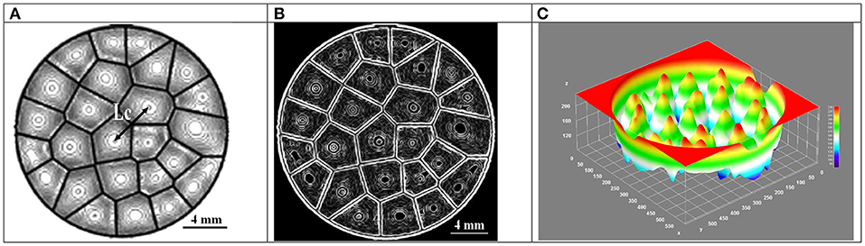
Figure 7. (A) Circulation cells in silicone oil layer (d = 2.1 mm) heated from below ΔT = 2.5 K, L_c = 2.3 × d = 4.9 mm. (B) “Find Edges” procedure (ImageJ program) applied to the picture. (C) 3D thermograph of liquid temperature distribution after onset of B-M circulation. Cooler and wormer regions are indicated with blue and red colors, respectively. When the pattern is fully developed, it becomes an almost perfect array of regular hexagons, arranged in a honeycomb.

By means of the image analysis procedure (Find Edges function in ImageJ program), hexagonal structures of B-M (Figure 7B) can be clearly visualized, whose characteristic cell sizes L_C (distance between the centers), remained in relation to the layer thickness L_C = 2.3 × d, consistent with the theoretical models and results of experiments (Chauvet et al., 2012). The gray intensity of black and white images is proportional to the temperature of the sample area that allowed to create a 3D image of the temperature distribution on the surface of the liquid (Figure 7C; Interactive 3D surface plot, ImageJ program), which exhibited the B-M pattern. Colder (blue) regions with higher surface tension are adjacent to warmer areas (red), where the surface tension is lowered. The surface tension gradient introduces an imbalance of forces, which causes liquid flow. The warmer fluid flows upward in the convection cell centers, while it is directed downwards at the hexagonal boundaries. When the mechanism reaches the steady state, the surface becomes an area entirely covered with almost ideal honey-like hexagons (Merkt and Bestehorn, 2003; Mancini and Maza, 2004).

The condition required to onset the B-M circulation is to achieve the threshold ΔT_c.

An interesting relationship between the Rayleigh and Rayleigh numbers can be obtained: Ra/Ma = (constant values characteristic of the probe liquid) × d², as a result the relative importance of the two effects involved in the B-M convection depends on the thickness of the liquid layer (Maroto et al., 2007). It is evident that the convection is controlled by surface tension forces for small thicknesses of the liquid layer. So surface tension effects are the predominant, although buoyancy forces become gradually important when the thickness of the liquid is increased. The critical ΔT_c temperature computed as a function of a model non-volatile liquid layer thickness (see Figure 5B in Maroto et al., 2007), established a decrease of the critical temperature gradient with the increment of the thickness of the liquid layer similarly as found in our experiments. Moreover, the temperature vertical gradient increase can make the flow beneath the expanding spill edge completely turbulent, as shown in Figure 2, and could be observed for the realistic case of low-temperature liquid spread over the warmer subphase.

The temperature difference ΔT_cool induced by the cooling process depends on the physical and thermal properties of the hydrocarbon related to the rate of evaporation (Chauvet et al., 2012; Machrafi et al., 2013).

The process of hydrocarbon evaporation considered in a larger spatial scale (at-sea) leads to the particular surface effects (Zhang, 2006), as illustrated in Figure 8.

FIGURE 8

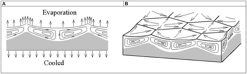
Figure 8. Temperature gradient circulating flow in an evaporating liquid layer cooled: (A) circulating flow induced by evaporation; (B) tessellation on the layer surface (Zhang, 2006).

In the case of evaporating liquid layers, there are local internal fluctuations and external disturbances (wind stresses, currents, and others) of random nature at the sea surface. A local increase in evaporation rate results in the drop of local temperature, and therefore creates a local increase of surface tension. The fluid from the adjacent area will be dragged toward this high surface tension region. The liquid coming from the surrounding area would push the local surface upward and make the surface ripples and corrugations. Meanwhile, the surface flow is communicated to the bulk of the fluid as a result of its shear viscosity and drags part of the bulk fluid upward. As it is known that the surface ripples and corrugations will enhance the local evaporation process, reinforcing the surface gradient in temperature and tension, and will amplify the local increase in the evaporation rate. Consequently, the evaporation rate at ridges of the cell surface would be higher than E at the center of the cell. The fluid transiting across the surface is cooled during its way and will sink at the region of the lowest temperature and the B-M circulation pattern is established. The isotherms and circulation flows in a cell are sketched in Figure 8.

The ocean surface is typically something like 0.1–0.6°C cooler than the temperature just below the surface. This “skin” or ultra-thin region is less than a 1 mm thick (Gentemann et al., 2009). Such a sea surface temperature (SST) difference can be quantified as:

$\begin{array}{ll}\Delta T_c=SS{T}_{skin}-T_{depth}=-0.14-0.3e^{(-U/3.7)},& (9)\end{array}$

where U is the wind speed in (ms⁻¹), as reported in Woods et al. (2014). For moderate winds i.e., U = 6 ms⁻¹, ΔT_c = −0.19°C. This value is higher than the threshold values ΔT_B−M theoretically predicted on the basis of thermophysical properties of all the considered liquids (see Table 1).

TABLE 1

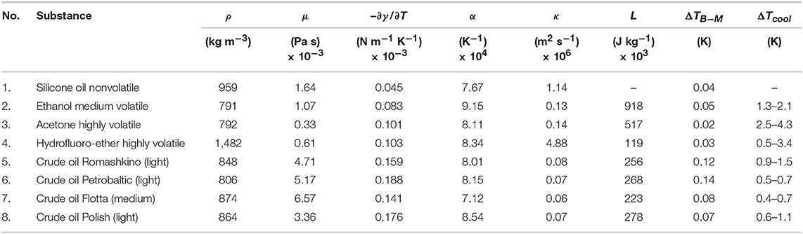
Table 1. Thermal and physical properties of studied liquids vs. critical threshold temperature difference ΔT_B−M predicted to onset B-M circulation in thin layers at ambient conditions (T = 23°C) and experimental evaporative cooling ΔT_cool.

Threshold B-M Circulation Temperature vs. Volatile Hydrocarbon Properties

The evaporation rate E = (dm/dt) was derived from the experimental curve (sample mass vs. evaporation time), depicted in Figure 9, for a very volatile hydrocarbon (acetone). In the initial stage, E-values equal to 0.16 ± 0.03 g min⁻¹ quickly decreased to 0.08 ± 0.01 g min⁻¹ as the air over the sample layer becomes saturated with acetone vapor at longer times. For liquids with medium volatility (ethanol), under the same experimental conditions, E = 0.032 ± 0.008 g min⁻¹.

FIGURE 9

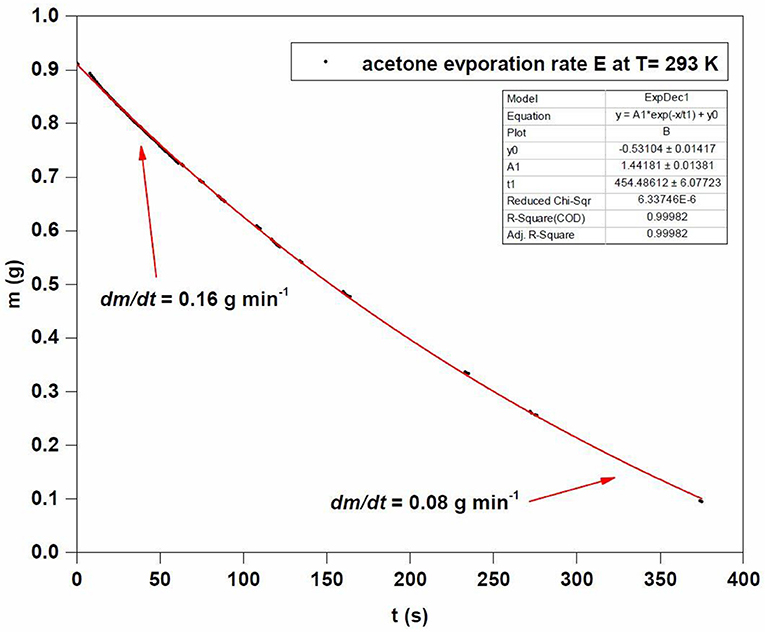
Figure 9. Evaporating sample mass vs. time dependence, and Acetone evaporation rate E = dm/dt at T = 23°C.

Theoretical work points to the following dependence for the threshold ΔT_cool on the physico-thermal parameters of the evaporating liquid related to E (Merkt and Bestehorn, 2003; Chauvet et al., 2012):

$\begin{array}{ll}\Delta T_{cool}~\mathrm{\text{Ed}}=\frac{ELd}{{\lambda }_{l}S},& (10)\end{array}$

where E is the evaporation rate, d is the liquid layer thickness, L is the latent heat of evaporation, λ_l is the liquid thermal conductivity (gas λ_g << λ_l liquid), S is the vessel cross-section area.

It is of particular value to quantify the evaporation rate of crude oil in at-sea conditions since it affects the threshold ΔT_cool. Evaporation is an important component in oil spill models (Fingas, 2012, 2013). The factors significant to evaporation include time and temperature. The difficulty in studying oil evaporation is that crude oil is a mixture of hundreds of compounds and oil composition varies from source to source and also over time. Evaporation equations are the principal physical change equations applied in spill models. The immediate layer of air above the evaporation surface, might be as thin as <1 mm, is called the boundary layer and in the case of water regulates the evaporation rate. Under low wind speed conditions or low turbulence, the air immediately above the water becomes saturated and evaporation slows. Under all experimental and environmental conditions, oil and petroleum products were not found to be boundary layer-regulated (Fingas, 2012). That is confirmed by a strong correlation between oil mass and evaporation rate (see Figure 6 in Fingas, 2012). The at-sea experiments showed a classical relationship between the water evaporation rate and the wind speed: E ~ U^0.78 (Fingas, 2013). Figures 1–4 in Fingas (2012) demonstrate that the evaporation rates for oils and even the light products, gasoline and heavy crude oil do not increase significantly with increasing wind. A comparison of the maximum evaporation rates for a few oils, gasoline, and water, measured under the wind-free condition showed that some oil rates exceeded that for water by as much as an order of magnitude (E_water = 0.034, light crude oil ASMB = 0.075, and Gasoline = 0.34 g min⁻¹ (Fingas, 2012) being in agreement with the E data obtained in this study. Further experiments performed by Yang and Wang (1997) showed that a film could be formed on evaporating oils and this compact, solid-like film significantly retarded evaporation. The evaporation rate turned out to be reduced fivefold after the surface film formation. An important factor of evaporation regulation is also the saturation concentrations which are collected in Table 1 of Fingas (2013), for water and several oil components. The saturation concentration of water is about two orders of magnitude less than the saturation concentration of volatile oil components such as pentane.

On the other hand, the direct measurement of ΔT_cool indicated the power-law like dependence: ΔT_cool = A·E^B, where A and B constants appeared to be dependent both on the thermal properties of hydrocarbons and air stream velocity over the evaporating surface. For evaporating crude oil and petroleum products, E is a wind speed U related quantity as found in field studies (Fingas, 2012).

The thermal and physical quantities that characterize the test liquids and raw crude oils together with the threshold values of ΔT_B−M (calculated from the theoretical model) and ΔT_cool measured experimentally in the evaporation process are summarized in Table 1. Temperature differences ΔT_cool registered in the process of evaporation for model liquids of significant volatility were of the order of 1.3–3.4 K but almost two times lower values (0.4–1.5 K) were found for crude oils. However, they are several times higher than the threshold ΔT_B−M theoretically-predicted values required for the B-M flow pattern to be initiated.

To sum up, the crude oil spreading at the final stage of the pollution expansion, when the surface tension forces play a main role is attributed to generation of subsurface turbulence dissipative flow of circular nature that leads to the slower velocity of the expanding oil front edge in reference to value predicted from the classical boundary-layer flow theory.

Apart from the thermal Marangoni effect, there is also the classic one, caused by the gradients of the concentration of natural surfactants present in the sea surface microlayer. The tangential stresses resulting from the both effects describe the dependence (Li and Mao, 2001; Pasquetti et al., 2002; Mao et al., 2008):

$\begin{array}{ll}{\tau }_z=\frac{\partial \gamma }{\partial c}·\frac{\partial c}{\partial z}+\frac{\partial \gamma }{\partial T}·\frac{\partial T}{\partial z}.& (11)\end{array}$

The first term (attributed to classical surfactant effect) ∂γ/∂z, reaches values from the range 5.32–10.45 mN m⁻², while the second one (thermal effect) in the Equation (11) is of the order of 52.6–274.2 mN m⁻², which is 10–30 times greater than that in the case of the surfactant-mediated effect, as found in thermo-elastic studies of Baltic Sea coastal waters (Boniewicz-Szmyt and Pogorzelski, 2016). The M-B circulation may be a very effective and still underestimated process of mixing, redistribution or enrichment of the micro-layer of the sea in various fractions of dissolved organic matter (DOM), in which temperature gradients (Marangoni's thermal effect) play a principal role, while the natural sea water surfactant effect is of secondary importance.

Conclusions

It is suggested that the decrease in the spreading exponent n (from ¾ to ½) in the relation r_L(t), observed for the volatile hydrocarbon films, occurring after 1–3 s from the moment of initiating the spread phenomenon, can result from the creation of Benard-Marangoni-type convective rolls which develop beneath the leading edge under particular conditions (sufficient evaporation rate, ΔT_coll cooling effect temperature difference between the free surface of the layer and the base). This highly dissipative nature of fluid flow, observed only in the case of volatile stretched films, leads to a significant decrease in the rate of expansion.

Large temperature gradients present in thin (~mm) liquid layers lead to perpendicular components of the U_s fluid velocities (0.1–0.3 cms⁻¹) that are responsible for the development of turbulent fluid circulation below the expanding film.

The threshold temperature difference ΔT_B−M required for the activation of B-M circulation pattern, determined on the basis of the thermo-physical properties of model substances, can be achieved by surface cooling for each of the tested hydrocarbon and the crude oils (ΔT_B−M << ΔT_cool).

The B-M circulation experiments performed here, for a non-volatile model liquid, established the threshold ΔT_c, which turned out to be much higher (a few K) than evaluated for the volatile liquids of the same layer thicknesses. For non-volatile crude oil products, the evaporative cooling mechanism of the B-M circulation is unlikely to appear, and the general dependence r_L ~ t^¾ is obtained at the latest stage of the oil spill spreading, where the “switch over” time was not observed as attributed to the transition from r_L ~ t^3/4 to t^0.5.

The temperature difference ΔT_cool, is a function of the evaporation rate ΔT_cool = A·E^B, where constants A and B depend on the velocity of the air stream over the evaporating liquid surface.

The generation of the Marangoni fluid flow mechanism in the upper per sea water microlayer is attributed mainly to temperature gradients with a minor role played by natural surfactant concentration gradients.

Fay's empirical formulas from layer-averaged Navier-Stokes equations and their later derivatives are still sometimes considered as the state-of-the-art in oil slick modeling literature. As argued in this preliminary study, the vertical fine processes are involved, and that a realistic model of oil dispersion should include vertical velocity shears.

In such a concept study, surface tension-dependent phenomena pointed to here are of universal concern in several physicochemical systems of oceanographic concern taking place at the interfaces (natural sea surface film formation, for instance) and turned out to be still underestimated effects.

Author Contributions

KB-S collected data in the field experiment, evaluated surface film parameters, performed correlation analyses, searched for literature background interpretation, and wrote manuscript. SP formulated work concept, created theoretical background, analyzed, and discussed results.

Funding

Support for this work was provided by the University of Gdansk (DS 530-5200-D-464-17).

Conflict of Interest Statement

The authors declare that the research was conducted in the absence of any commercial or financial relationships that could be construed as a potential conflict of interest.

References

Adamson, A. W., and Gast, A. P. (1997). Physical Chemistry of Surfaces. New York, NY: John Wiley and Sons.

Google Scholar

Bauget, F., Langevin, D., and Lenormand, R. (2001). Dynamic surface properties of asphaltenes and resins at the oil-water interface. J. Colloid Interface Sci. 239, 501–508. doi: 10.1006/jcis.2001.7566

CrossRef Full Text | Google Scholar

Bejan, A. (2004). Convection Heat Transfer. New York, NY: Wiley and Sons.

Google Scholar

Berg, S. (2009). Marangoni-driven spreading along liquid-liquid interfaces. Phys. Fluids 21, 032105–032112. doi: 10.1063/1.3086039

CrossRef Full Text | Google Scholar

Boniewicz-Szmyt, K., and Pogorzelski, S. J. (2008). Crude oil derivatives on sea water: signatures of spreading dynamics. J. Mar. Syst. 74, S4S1–S5S1. doi: 10.1016/j.jmarsys.2007.11.015

CrossRef Full Text | Google Scholar

Boniewicz-Szmyt, K., and Pogorzelski, S. J. (2016). Thermoelastic surface properties of seawater in coastal areas of the Baltic Sea. Oceanologia 58, 25–38. doi: 10.1016/j.oceano.2015.08.003

CrossRef Full Text | Google Scholar

Boniewicz-Szmyt, K., Pogorzelski, S. J., and Mazurek, A. (2007). Hydrocarbons on sea water: steady-state spreading signatures determined by an optical method. Oceanologia 49, 413–437.

Google Scholar

Camp, D. W., and Berg, J. C. (1987). The spreading of oil on water in the surface tension regime. J. Fluid Mech. 184, 445–462.

Google Scholar

Chauvet, F., Dehaeck, S., and Colinet, P. (2012). Threshold of Benard-Marangoni instability in drying liquid films. Europhys. Lett. 99:34001. doi: 10.1209/0295-5075/99/34001

CrossRef Full Text | Google Scholar

Craster, R. V., and Matar, O. K. (2006). On the dynamics of liquid lenses. J. Colloid Interface Sci. 303, 503–516. doi: 10.1016/j.jcis.2006.08.009

PubMed Abstract | CrossRef Full Text | Google Scholar

Dussaud, A. D., and Troian, S. M. (1998). Dynamics of spontaneous spreading with evaporation on a deep fluid layer. Phys. Fluids 10, 23–38.

Google Scholar

Elliott, A. (1986). Shear diffusion and the spread of oil in the surface layers of the North Sea. Dt.Hydrogr.Z. 39, 113–137.

Google Scholar

Fingas, M. F. (2012). Studies on the evaporation regulation mechanisms of crude oil and petroleum products. Adv. Chem. Eng. Sci. 2, 246–256. doi: 10.4236/aces.2012.22029

CrossRef Full Text | Google Scholar

Fingas, M. F. (2013). Modeling of oil and petroleum evaporation. J. Petrol. Sci. Res. 2, 104–115.

Google Scholar

Gentemann, C. L., Minnett, P. J., and Ward, B. (2009). Profiles of ocean surface heating (POSH): a new model of upper ocean diurnal warming. J. Geophys. Res. 114:C0C7017. doi: 10.1029/2008J88JC0C004825

CrossRef Full Text | Google Scholar

Giwa, A., and Jimoh, A. (2010). Development of models for the spreading of crude oil. AU J.T. 14, 66–71.

Google Scholar

Hibiya, T., and Ozawa, S. (2013). Effect of oxygen partial pressure on the Marangoni flow of molten metals. Cryst. Res. Technol. 48, 208–213. doi: 10.1002/crat.201200514

CrossRef Full Text | Google Scholar

Jones, J. C. (2010). Hydrocarbons- Physical Properties and Their Relevance to Utilization. Houston, TX: Jones and Ventus Publishing ApS.

Google Scholar

Lehr, W. J., and Simecek-Beatty, D. (2000). The relation of Langmuir circulation processes to the standard oil spill spreading, dispersion, and transport. Spill Sci. Technol. Bull. 6, 247–253. doi: 10.1016/S1353-2561(01)00043-3

CrossRef Full Text | Google Scholar

Li, X. J., and Mao, Z. S. (2001). The effect of surfactant on the motion of buoyancy-driven drop at intermediate Reynolds numbers: a numerical approach. J. Colloid Interface Sci. 240, 307–322. doi: 10.1006/jcis.2001.7587

CrossRef Full Text | Google Scholar

Machrafi, H., Sadoun, N., Rednikov, A., Dehaeck, S., Dauby, P. C., and Colinet, P. (2013). Evaporation rates and Benard-Marangoni supercriticality levels for liquid layers under an inert gas flow. Microgravity Sci. Technol. 25, 251–265. doi: 10.1007/s12217-013-9355-8

CrossRef Full Text | Google Scholar

Mancini, H., and Maza, D. (2004). Pattern formation without heating in an evaporative convection experiment. Europhys. Lett. 66, 812–818. doi: 10.1209/epl/i2003-10266-0

CrossRef Full Text | Google Scholar

Mao, Z., Lu, P., Zhang, G., and Yang, C. H. (2008). Numerical simulation of the Marangoni effect with interphase mass transfer between two planar liquid layers. Chin. J. Chem. Eng. 16, 161–170. doi: 10.1016/S1004-9541(08)60057-9

CrossRef Full Text | Google Scholar

Maroto, J. A., Perez-Munuzuri, V., and Romero-Cano, M. S. (2007). Introductory analysis of Benard-Marangoni convection. Eur. J. Phys. 28, 311–320. doi: 10.1088/0143-0807/28/2/016

CrossRef Full Text | Google Scholar

Merkt, D., and Bestehorn, M. (2003). Benard-Marangoni convection in a strongly evaporating fluid. Physica D 185, 196–208. doi: 10.1016/S0167-2789(03)00234-3

CrossRef Full Text | Google Scholar

Njobuenwu, D. O., and Abowei, M. F. N. (2008). Spreading of oil spill on placid aquatic medium. Leonardo J. Sci. 7, 11–24.

Google Scholar

Pasquetti, R., Cerisier, P., and LeNiliot, C. (2002). Laboratory and numerical investigations on Benard-Marangoni convection in circular vessels. Phys. Fluids 14, 227–228. doi: 10.1063/1.1424307

CrossRef Full Text | Google Scholar

Pearson, J. R. A. (1958). On convection cells induced by surface tension. J. Fluid Mech. 4, 489–496.

Google Scholar

Perfetti, C., and Iorio, C. S. (2014). Evaporation induced thermal patterns in fluid layers: a numerical study. J. Electr. Cool. Therm. Cont. 4:52049. doi: 10.4236/jectc.2014.44011

CrossRef Full Text | Google Scholar

Riazi, M. R. (2005). Characterization and Properties of Petroleum Fractions. Philadelphia, PA: ASTM International.

Google Scholar

Sefiane, K., and Ward, C. A. (2007). Recent advances on thermocapillary flows and interfacial conditions during the evaporation of liquids. Adv. Colloid Interface Sci. 134–135, 201–223. doi: 10.1016/j.cis.2007.04.020

PubMed Abstract | CrossRef Full Text | Google Scholar

Toussaint, G., Bodiguel, H., Dumenc, F., Guerrier, B., and Allain, C. (2008). Experimental characterization of buoyancy- and surface tension-driven convection during the drying of a polymer solution. Int. J. Heat Mass Transfer 51, 4228–4237. doi: 10.1016/j.ijheatmasstransfer.2008.02.006

CrossRef Full Text | Google Scholar

Unny, T., and Niessen, P. (1969). Thermal instability in fluid layers in the presence of horizontal and vertical temperature gradients. J. Appl. Mech. 36, 121–128.

Google Scholar

Woods, S., Minnett, P. J., Gentemann, C. L., and Bogucki, D. (2014). Influence of the ocean cool skin layer on global air-sea CO₂O flux estimates. Remote Sens. Environ. 145, 15–24. doi: 10.1016/j.rse.2013.11.023

CrossRef Full Text | Google Scholar

Yang, W. C., and Wang, H. (1997). Modelling of oil evaporation in aqueous environment. Water Res. 11, 879–887.

Google Scholar

Yoda, Y. (2007). Research Report NSR. Japan Chemical Society.

Google Scholar

Zhang, N. (2006). “Surface tension-driven convection flow in evaporating liquid layers,” in Surface Tension-Driven Flows and Applications, ed R. Savino (Trivandrum: Research Signpost), 147–170.

Google Scholar