Designating Spatial Priorities for Marine Biodiversity Conservation in the Coral Triangle

Introduction

The continuing trend of biodiversity loss as a result of various human activities and climate change is likely to have serious ecological, social, and economic implications (Cardinale et al., 2012; Hooper et al., 2012; Halpern B.S. et al., 2015). In the last four decades, there has been a decline in the abundance of 58% of global vertebrate species populations and about 31% of marine fauna (WWF, 2016) and scientists suggest that a sixth mass extinction event may be underway (Barnosky et al., 2011). In the ocean, these declines may affect human well-being through imperiling food security and reducing the ecosystem services provided (Costello and Baker, 2011; McCauley et al., 2015). Globally, coral reefs support more than 250 million people and protect the coastline of more than a hundred countries, but are threatened by various human-induced pressures (Burke et al., 2012). However, neither marine biodiversity nor the threats to it are evenly distributed, and limited resources are available to adequately protect all of the important biodiversity features (Brooks, 2014; Pimm et al., 2014). These aforementioned challenges have led to the adoption of systematic conservation-planning approaches to guide efficient investment to ensure the representation and long-term persistence of biodiversity (Pressey et al., 1993; Margules and Pressey, 2000; Brooks, 2010).

Two key metrics that have been widely used in conservation prioritization are irreplaceability (degree of uniqueness) and vulnerability (degree of threat) (Margules and Pressey, 2000; Langhammer et al., 2007; Edgar et al., 2008; Brooks, 2010). These two metrics work in parallel to identify high priority areas for biodiversity conservation (Pressey et al., 1993). High irreplaceability exists if one or more key habitats or species are constrained to particular areas, and there are only a few spatial options for protecting that species. High vulnerability means that there is an imminent threat to the persistence of biodiversity that calls for immediate conservation action (Langhammer et al., 2007). Thus, to prevent biodiversity loss, conservation actions are required immediately in areas where there are limited spatial and temporal replacement options (Pressey et al., 1994; Rodrigues et al., 2004). The degree of uniqueness of an area may be measured through suites of ecological and biological criteria that capture the significant biodiversity values based on habitat-specific attributes (e.g., areas that contain unique, rare, fragile, and sensitive habitats) and/or species-specific attributes (e.g., the presence of the species of conservation concern or restricted-range species) (Roberts et al., 2003a; Hiscock, 2014; Asaad et al., 2016). The degree of threat may be evaluated through a series of pressure factors (e.g., destructive fishing, pollution, and rising sea surface temperature) that may prevent ecosystems from delivering their services and functioning properly (Halpern et al., 2008; van Hooidonk et al., 2016).

The methods to prioritize areas important for biodiversity conservation have evolved from ad hoc and opportunistic to systematic and scientific-based approaches (Stewart et al., 2003). A systematic approach can be applied by iterative evaluation of pre-determined criteria (Day et al., 2000), applying mathematical site-selection algorithms (Hiscock, 2014), or a combination of those two approaches (Roberts et al., 2003b). Compared to ad hoc approaches, systematic approaches provide flexibility to compare different options of protected area scenarios and allow a systematic consideration of protected areas goals and objectives (Roberts et al., 2003b). Clark et al. (2014) explored the application of multiple ecological criteria (e.g., criteria of unique and rare habitats, threatened species, and critical habitats) to identify ecologically and biologically significant areas in the South Pacific Ocean. Sala et al. (2002) applied site-selection algorithms based on multiple levels of information on ecological processes (e.g., spawning, recruitment, and larval connectivity) and objectives (e.g., identifying 20% of representative habitat and 100% of rare habitats) to evaluate candidate protected areas in the Gulf of California. A similar approach was used by Fernandes et al. (2005) to identify representative no-take areas that included a minimum of 20% of each “bioregion” in the Great Barrier Reef Marine National Park of Australia. White J.W. et al. (2014) tested a range of reserve configurations using biological criteria (i.e., habitat, self-retention, and centrality) to optimize fish biomass. Further, Magris et al. (2017) developed a marine protected area (MPA) zoning system to accommodate multiple sets of conservations objectives (i.e., representing biodiversity features, maintaining connectivity, and addressing climate change impact) for Brazilian coral reefs. Such a selection process can be facilitated by the application of conservation prioritization software such as Marxan (Ball et al., 2009; Watts et al., 2009), C-Plan (Pressey et al., 2009), Zonation (Moilanen et al., 2005, 2009, 2011), and other spatial decision support tools.

Spatial prioritization methods for systematic conservation planning have been applied to evaluate protected area networks (Leathwick et al., 2008), to inform expansion of protected areas (Pouzols et al., 2014), and to identify gaps in biodiversity conservation (Sharafi et al., 2012; Jackson and Lundquist, 2016; Veach et al., 2017). An understanding of the underlying biodiversity patterns is required to identify priority areas and to design optimal scenarios for biodiversity conservation. Several studies have suggested using species richness metrics (e.g., abundance, range rarity, and range size) (Brooks et al., 2006; Jenkins et al., 2013; Pimm et al., 2014), while others integrate biodiversity conservation scenarios with climate change (Schuetz et al., 2015; Magris et al., 2015) and economic objectives (Geange et al., 2017).

The Coral Triangle (CT) Region is a marine area that encompasses parts of South-East Asia and the Western Pacific. Its sea area is larger than that of the European Atlantic and Mediterranean combined (Costello et al., 2010). Known as the global epicenter of shallow marine biodiversity for its high species richness and endemicity, the region contains more than 76% of the world’s shallow-water reef-building coral species (Veron et al., 2009), 37% of the world’s reef fishes (Allen, 2008), six out of seven of the world’s sea turtles and the largest mangrove forest in the world (Polidoro et al., 2010; Walton et al., 2014). Scientists have proposed an ecological boundary of the CT based upon the 500 species isopleth for reef-building coral species richness (e.g., Green and Mous, 2008; Veron et al., 2009). In addition, six countries within the CT region (Indonesia, Malaysia, Papua New Guinea, the Philippines, Solomon Islands, and Timor-Leste) have declared their commitments to working collaboratively to safeguard their marine resources through a multilateral partnership known as the CT Initiative (CTI-CFF, 2009; Figure 1).

FIGURE 1

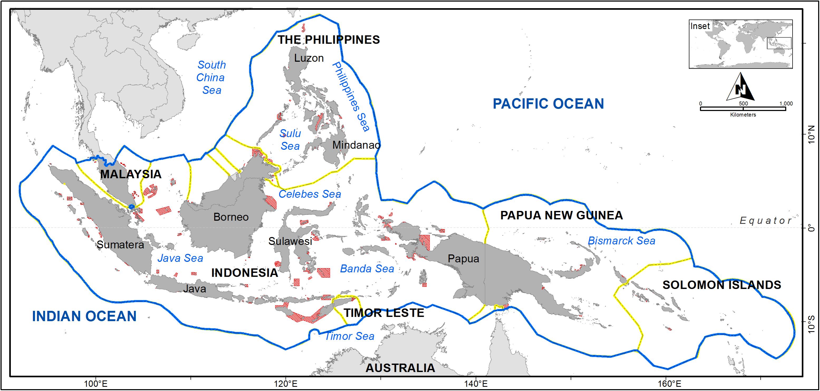
FIGURE 1. The six Coral Triangle (CT) Initiative countries and marine protected areas (MPAs) (red) within their extended Economic Exclusive Zone (blue line). Country boundaries are indicated by a yellow line.

More than 1,900 MPAs covering an area of 200,881 km² have been established within the CT (Cros et al., 2014b). This current protection equates to less than 2% of the CT marine areas and is predominantly located in coastal waters (Cros et al., 2014a; White A.T. et al., 2014). Underrepresentation of ecological and biodiversity coverage occurs in the region, where it was estimated that only 14.7% of coral reefs and 5.4% of mangroves in the CT are located within protected areas (Beger et al., 2013). In Indonesia, only 49% of sea turtle and 44% of dugong important habitats have been declared protected areas (MoF-MoMAF, 2010). Most of these MPAs were established in the mid-1990s, with a primary objective of biodiversity preservation (Green et al., 2011; White A.T. et al., 2014) and limited consideration of incorporating other objectives (e.g., fisheries management or climate change adaptation) (Green et al., 2014) or to be adaptive to environmental change (Anthony et al., 2015).

In the CT, earlier spatial prioritization exercises were typically focused on national geographies. In Indonesia, the most recent national marine biodiversity prioritization was developed based on species richness and endemism (Huffard et al., 2012), whereas a recent Philippines prioritization was based on habitats of threatened species (Ambal et al., 2012). Using biodiversity features and a climate change index, Beger et al. (2015) conducted a biodiversity prioritization scenario that covered the coastal areas of the CT, though this prioritization did not take into account anthropogenic pressures (APs) (with the exception of climate change) that are considered to be the main threats to biodiversity conservation in the CT region. To protect a representative range of marine biodiversity in a system of MPAs, the CT countries could develop and expand their MPA system to fulfill their obligations to the Convention on Biological Diversity (CBD) – Aichi Biodiversity Target 11 (Convention on Biological Diversity, 2010), and to achieve Goal 14 of the United Nations – Sustainable Development Goals. The CT countries have set a target that by 2020, at least 10% of the CT critical marine habitats will be protected within no-take reserves and 20% will be included in some form of MPA (CTI-CFF, 2013). Therefore, it is timely to demonstrate the application of spatial conservation prioritization to support CT national commitments toward effective MPA system design, and how well these targets would protect biodiversity.

In this study, we explored the application of spatial decision support tools for conservation planning to guide the identification of an effective MPA system for the CT. This represents the largest geographic area where a systematic process based on empirical data has been used to inform selection of MPAs. Previously, we identified important areas of marine biodiversity conservation in the CT based on five ecological criteria: sensitive habitats, species richness, the presence of species of conservation concern, the occurrence of restricted-range species, and areas important for critical life history stages (Asaad et al., 2018). Herein we utilize those previously identified criteria in performing a comprehensive assessment of priority areas for expanding the current CT MPA system. We evaluate the efficiency of the current CT MPA system in protecting a representative range of selected biodiversity features and then present a prioritization scenario for expanding the MPA system based on the integration of biodiversity features and present anthropogenic and projected climate change pressures. Our assessment and analyses provide a strategy for the CT countries to focus their efforts and resources on prioritizing, expanding and managing MPAs that potentially deliver the greatest contribution to preserving the region’s unparalleled marine biodiversity.

Materials and Methods

Study Area

The study area is the CT region, as defined by the official implementation area for the CT Initiative. This boundary covers the entire Exclusive Economic Zones (EEZs) of Indonesia, Malaysia, Papua New Guinea, the Philippines, Solomon Islands, and Timor-Leste, and also includes the EEZs of two adjacent nations: Brunei Darussalam and Singapore (Figure 1). While this study area is slightly larger than the CT sensu stricto, this larger region is most appropriate for our analyses, as the countries involved focus their conservation policies and planning based on political boundaries rather than biological boundaries such as the one that strictly defines the CT based on hard coral diversity isopleths (e.g., Veron et al., 2009).

Although our regional maps and analysis included the EEZ of eight countries in the region, we focused our regional summary statistics only to the six CT countries. Two countries (Brunei Darussalam and Singapore) have relatively small EEZs, and the spatial resolution of our models provided limited information to differentiate biodiversity priorities in these EEZs.

Datasets

We used five ecological criteria synthesized by Asaad et al. (2016), namely: sensitive habitats, species richness, the presence of species of conservation concern, the occurrence of restricted-range species, and areas important for life history stages to evaluate the performance of an existing MPA system in protecting representative ranges of biodiversity features and develop a prioritization scenario for expansion of the MPA system. Further, we used a variety of datasets to inform our analysis (Table 1). The dataset of biodiversity features was comprised of biodiversity feature maps compiled by Asaad et al. (2018). Following Asaad et al. (2016), the definitions of each criterion were as follows:

TABLE 1

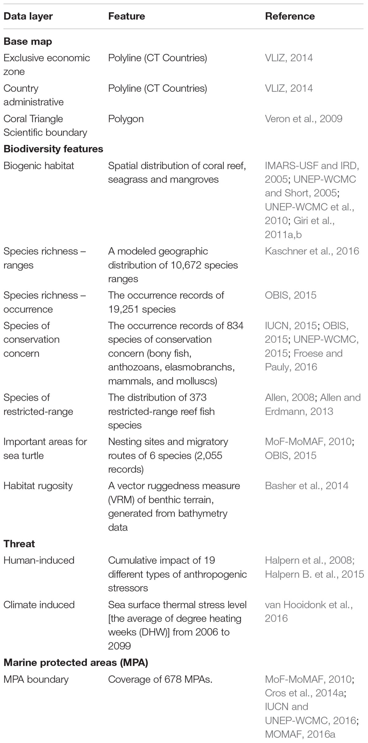
TABLE 1. Summary of data sources used in this study.

§Sensitive habitat: this criterion defines habitats that are relatively susceptible to natural or human-induced threats. Protecting such areas may help reduce disturbance from humans. To assess this criterion, we used spatial distributions of three biogenic habitats (coral reefs, seagrass meadows, and mangrove forests).

§Species richness: this criterion defines areas that are inhabited by a large number of species. This criterion was assessed using modeled geographic species distributions and point occurrence records of more than 10,000 species. In this study, species richness was quantified as the sum of presences of all species from (i) species distribution models (species ranges derived from modeled geographic distributions, retrieved from the AquaMaps dataset) and (ii) species occurrence records (retrieved from OBIS datasets) to allow inclusion of the maximum complement of biodiversity. For the species ranges, richness was based on the number of predicted species in each cell. For the species occurrence records, ES₅₀ (estimated species in random 50 samples) were calculated based on Hurlbert’s index of expected species richness (Hurlbert, 1971) and Hurlbert’s standard errors (Heck et al., 1975). We note that the first dataset is prone to commission errors (false positives) and the latter by omission errors (false negatives).

§Species of conservation concern: this criterion defines areas that are inhabited by species that are categorized as threatened or protected (e.g., listed in the IUCN Red List of Threatened species, CITES Appendix, EU Bird and Habitat Directive Annex or other regional/national legislations). This criterion was assessed using a summed layer of distributions of more than 800 species of special conservation concern.

§Restricted range species: this criterion defines areas inhabited by species that have restricted geographic distributions. In this study, this criterion was assessed using the distributions of 373 endemic reef fish species, each of whose entire geographic range is contained within the CT.

§For the criterion of area that is important for critical life history stages, we used sea turtle nesting habitat and migratory routes as indicators of important areas for sea turtles.

The dataset of a vector ruggedness measure (VRM) of benthic terrain was analyzed to measure benthic terrain rugosity and topographic ruggedness as an indicator of benthic habitat heterogeneity. This dataset covers the entire study area whereas our biogenic habitats data have only been estimated from the coastal zone. A VRM is a geomorphological index based on 3-dimensional dispersions of vectors normal (orthogonal) to a planar surface (Hobson, 1972; Sappington et al., 2007). To quantify this index, we extracted bathymetry data from GMED (Global Marine Environment Datasets) (Basher et al., 2014) and analyzed it using the Benthic Terrain Modeler (BTM) 3.0 of ArcGIS 10.5 (Wright et al., 2012). The benthic rugosity index has been applied as a proxy for benthic habitat heterogeneity, and greater habitat heterogeneity is associated with greater benthic species richness (Wilson et al., 2007; Harris and Baker, 2012).

The spatial distribution of AP to marine environments was retrieved from the database of cumulative human impacts on the world’s oceans developed by Halpern B.S. et al. (2015). This dataset was based on the cumulative impact of 19 different types of anthropogenic stressors: land-based drivers (nutrient inputs, organic and inorganic pollution, and population density), ocean-based drivers (commercial fishing, artisanal fishing, benthic structures, shipping lanes, invasive species, and pollution), and climate change (sea level rise, sea surface temperature anomalies, ultraviolet radiation and acidification) (Halpern et al., 2008; Halpern B. et al., 2015; Halpern B.S. et al., 2015). With a data resolution of ∼1 km², the dataset can be used to identify areas that are either relatively pristine or heavily impacted by human-induced stressors.

The dataset of the sea surface thermal stress level was derived from van Hooidonk et al. (2016). This dataset was based on the average of degree heating weeks (DHW) from 2006 to 2099. DHW is a measurement to assess patterns of sea surface temperature (SST) variability by combining the intensity and duration of thermal stress in order to predict coral bleaching (Liu et al., 2003). To generate the projections, monthly data of SST were obtained from 33 Coupled Model Inter-comparison Project 5 (CMIP5) for Representative Concentration Pathways 8.5 (RCP 8.5) experiments (Moss et al., 2010; Riahi et al., 2011). For the statistical downscaling, model outputs were adjusted to the mean and annual cycle of observations of SST based on the NOAA Pathfinder v.5.0 year 1982–2008 climatology, which has a 4-km resolution (Casey et al., 2010). Degree heating months were calculated for each year between 2006 and 2099 as anomalies above the warmest monthly temperature (the maximum monthly mean or MMM) from the Pathfinder climatology, and were summed for each period of three consecutive months in the time series. Degree heating months were converted into DHW by multiplying by 4.35 (Donner et al., 2005; van Hooidonk et al., 2014, 2015). The RCP8.5 scenario was used as it has the highest greenhouse gas emission and characterizes the current emission trajectory.

To estimate existing MPA protection, we combined data from the World Database of Protected Areas-WDPA¹ (IUCN and UNEP-WCMC, 2016), the CT Atlas² (Cros et al., 2014a) and the Indonesian database of MPAs (MoF-MoMAF, 2010; MOMAF, 2016a). The WDPA was amended with additional data from the CT Atlas. The most authoritative source for Indonesia was considered to be its government sources. This dataset consisted of 678 MPA boundaries in a polygon format which represented 35% of the total 1,972 MPAs in the region (White A.T. et al., 2014). We excluded MPAs which had missing boundaries or were represented only by point locations (longitude and latitude coordinates) as they may reduce the validity and tend to commission errors. Around 60% of the missing MPA boundaries were associated with very small village-based marine managed areas located predominantly in the Philippines (Venegas-Li et al., 2016). Importantly, the total coverage of MPA summed over the available polygon boundaries (240,443 km²) is larger than the total coverage of MPA officially reported by the CT countries (200,881 km²) (White A.T. et al., 2014). The discrepancy in MPA coverage occurs as some protected areas have both terrestrial and marine components (e.g., coastline, beaches, or small islands), and there were inconsistencies between the official documents and the accompanying GIS spatial boundary datasets. Of the 678 MPAs, less than 8% were fully protected (e.g., nature reserve and wildlife sanctuaries), 7% were multiple zone national parks, and the rest were categorized as nature recreation parks, protected seascapes, or locally managed marine areas (Supplementary Table S1).

ArcGIS 10.5 (ESRI, 2016) was used for all of the spatial data preparations, including spatial conversion, rasterization, and reclassification. All of the datasets were referenced to a geographic system of WGS84 (World Geodetic Survey 1984) with a Cylindrical Equal Area projection, and converted to a raster grid of a 500 m spatial resolution. We opted to subsample and downscale all of the datasets to a high spatial resolution in order to have a consistent spatial resolution across the datasets and to align with the small-sized MPAs within the CT.

Analysis of Threats

We evaluated the vulnerability of the CT to two threats: present anthropogenic and projected climate change pressures. Within the CT, the AP value ranged from 0 to 15.4. To compare the AP index across the CT, we categorized the AP value into low, medium and high based on the mean and standard deviation of the data. The mean was 3.9, and the standard deviation was 0.8. Low vulnerability areas were defined as those with AP values <3.1 (the mean less the standard deviation); medium vulnerability 3.1–4.8; and high vulnerability >4.8 (the mean plus the standard deviation).

A similar approach was used for the vulnerability to climate change pressure by binning the values into low, medium and high vulnerability. The projected thermal stress index based on DHW ranged from 5.6 to 20.2, with a mean of 15.9, and the standard deviation was 1.2. In this case, we defined areas with low vulnerability to climate change pressure as those with DHW values <14.8; medium vulnerability 14.8–17.2; and high vulnerability >17.2.

Spatial Conservation Prioritization

We used the Zonation software for spatial conservation prioritization to prioritize representative areas for biodiversity conservation. The Zonation meta-algorithm is a reverse stepwise heuristic that begins by assuming that the landscape is fully protected, and then progressively identifies and removes cells that contribute to smallest marginal losses in the representation of biodiversity features (Moilanen et al., 2005, 2009, 2011; Lehtomäki and Moilanen, 2013). Zonation results in a prioritization hierarchy; these priority values were then used to identify locations that contributed most to biodiversity representation.

We evaluated the effects of different scenarios on the distribution of priority locations for six biodiversity features and the rugosity indicator of habitat heterogeneity. We conducted three scenario analyses: (1) a biodiversity-optimized scenario, hereafter “Biodiversity-optimized”; (2) a scenario incorporating the protection of biodiversity features provided by existing protected areas, hereafter “Existing Protection”; and (3) a scenario revising priorities for biodiversity protection based on information on anthropogenic threats and climate change, hereafter “Threat”. The “Biodiversity-optimized” scenario used the six biodiversity feature layers and rugosity to design priority areas and identifies the maximum potential biodiversity feature representation for a given percentage of the total CT area protected. The “Existing Protection” scenario was derived from the “Biodiversity-optimized” analysis through the addition of an existing MPA layer as a removal mask to estimate the proportion of biodiversity features represented within the current MPA system in the CT. The “Threat” scenario further expanded on scenarios one and two by incorporating two types of threat (anthropogenic and climate-induced pressure) as indicators of vulnerability. Threat layers were assigned a negative weighting as biodiversity features in Zonation, allowing Zonation to use the ranked values of vulnerability to threats in the prioritization to avoid areas with a high likelihood of threats and thus reduced long-term resilience. We note that for some of the anthropogenic stressors included in the international threat layer (e.g., extractive resources uses), this analysis results in the selection of areas that minimize overlap with these uses which increase vulnerability of biodiversity. Selection via trade-offs with extractive uses can be perceived to be avoiding conflict, as should the extractive use be prevented in an MPA, the threat would be removed and species would be less vulnerable.

Zonation offers several cell-removal rules to aggregate marginal loss of conservation value (Moilanen, 2007; Moilanen et al., 2011). We chose to implement the Additive Benefit Function (ABF) analysis (Moilanen, 2007) as this cell-removal rule tends to emphasize areas with high biodiversity richness and our biodiversity metrics were summaries of multiple biodiversity features more representative of species richness than of individual species distributions (for which other Zonation cell-removal rules would be more appropriate). ABF allows for trade-offs among cells depending on how many biodiversity features occur in each cell, as well as the proportion of each feature remaining in other parts of the landscape (Moilanen et al., 2011, 2014). We used optional tools of Zonation including an edge removal rule (Moilanen, 2007), where cells from the edge of the remaining landscape were eliminated first, which increases aggregations of high-quality areas within the landscape. All of the results were evaluated based on the aggregate measures of performance that summarize statistics describing the quality, extent, and spatial distributions of biodiversity features within the region (Moilanen, 2007). Scenarios were compared to determine the average representation of biodiversity features within the existing MPA system relative to the potential protection that could be achieved with no constraints based on existing protected area boundaries. Further analyses compared changes in the proportion of biodiversity features protected and the spatial distribution of priority areas with increasing proportions of the CT region placed into an MPA system. That is, it projected the expansion of the MPA system in the CT from the present 1.8–10%, 20%, and 30% of the combined EEZ area. The “Threat” scenario was performed both on the full CT EEZ region, and individually on each of the national EEZs to determine differences between regional and national analyses and to inform national Aichi target objectives.

Results

Spatial Distribution of Biodiversity Features and Threat

We found that biogenic habitats of coral reefs, seagrass, and mangroves were distributed in over 9% of the CT. The modeled geographic species distribution of over 10,000 species showed that the number of predicted species in a given cell in the CT area ranged from 0 to 5,509 species. Species richness in the CT based on the index of expected species richness ES₅₀ (estimated species in 50 random samples) ranged from 1.6 to 49, indicating areas of low to high species richness. The distributions of 373 species of restricted-range reef fishes indicated that the total number of restricted-range reef fishes present in a given cell ranged from 0 to 101 species. More than 50% of the CT was identified as either nesting grounds or migratory routes of sea turtles. The vector ruggedness measures (VRMs) showed that the rugosity value of the CT ranged from 0.1 (areas with low terrain variations) to 0.9 (areas with very high terrain variations) (Figures 2A–G).

FIGURE 2

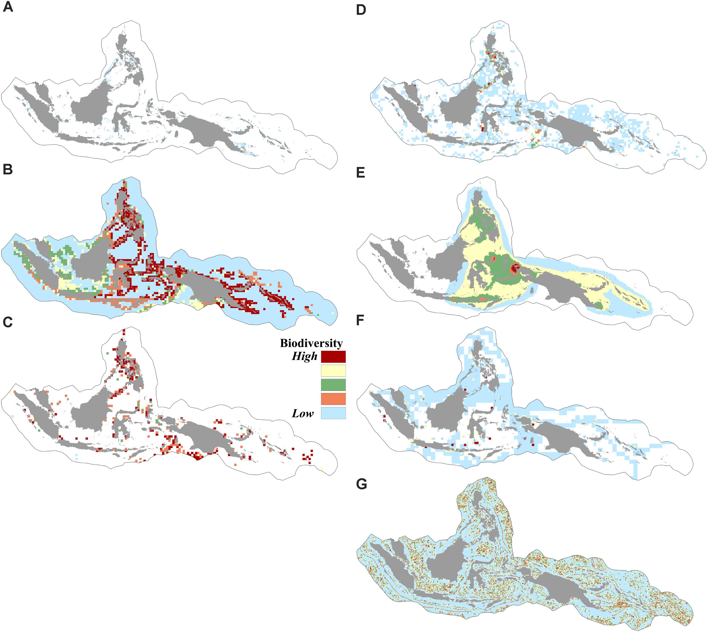
FIGURE 2. Spatial distribution of biodiversity features: (A) coverage of coral reefs, mangroves, and seagrasses, (B) modeled geographic ranges of 10,672 species, (C) richness (occurrences) based on ES50 of 19,251 species, (D) richness of species of conservation concern based on ES35 of 834 species, (E) distribution of 373 restricted range reef fishes, (F) distribution of six sea turtle species, (G) habitat rugosity based on the vector ruggedness measure of benthic terrain.

Vulnerability to Human and Climate-Induced Stressors

Approximately 36% of the CT was categorized as subject to low anthropogenic pressure (AP index <3.1), and more than 50% the CT was categorized as high (AP index >4.8). Areas of high anthropogenic pressure were concentrated predominantly in the central part of the Philippines, South China Sea, Malacca Strait, and Java Sea (Figures 3A, 4A).

FIGURE 3

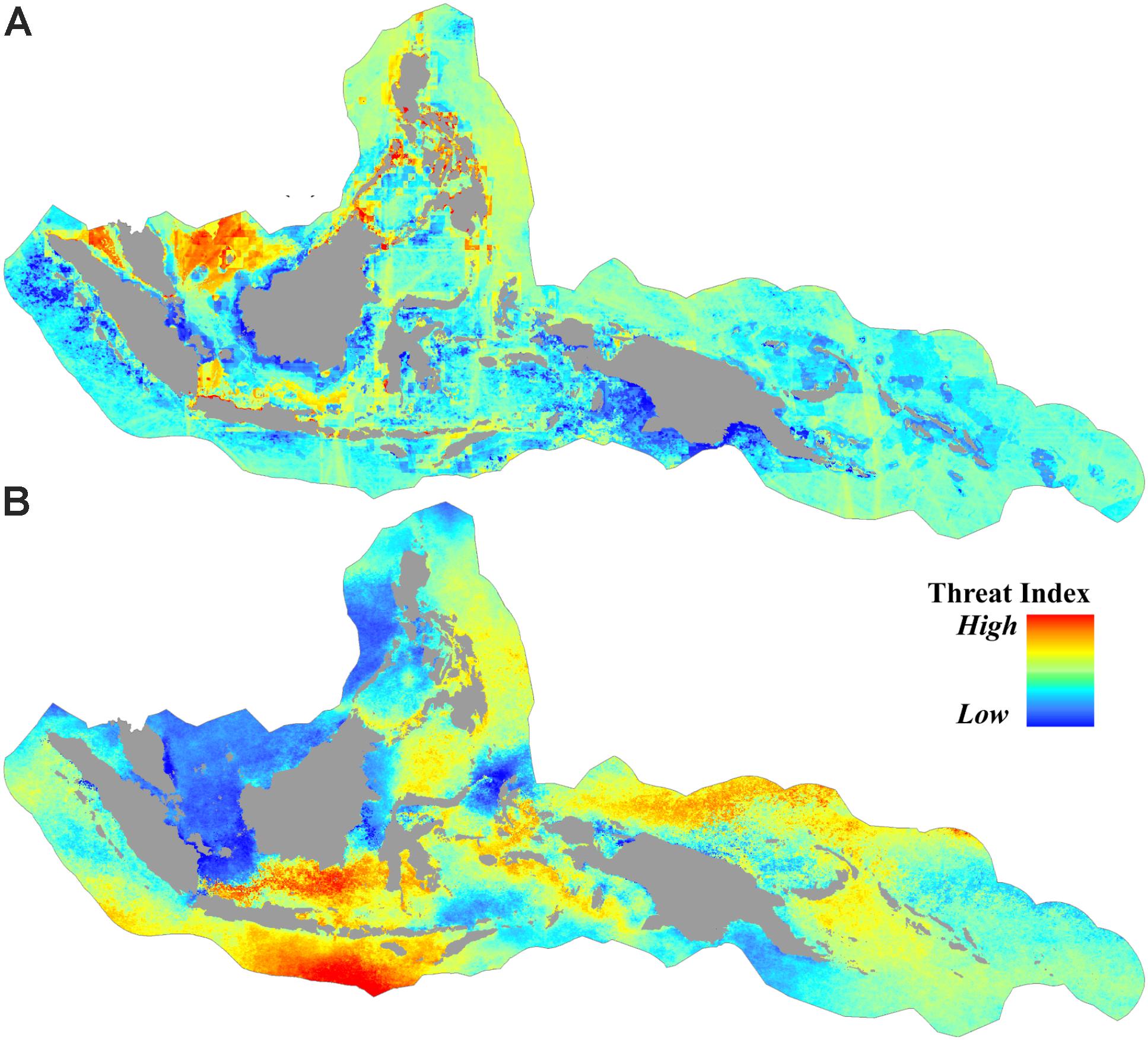
FIGURE 3. Spatial distribution of threats from (A) anthropogenic pressures based on the cumulative human impact to the marine environment, and (B) sea surface thermal stress based on the average of projected degree heating weeks (DHW) (year 2006 to 2099) under RCP8.5.

FIGURE 4

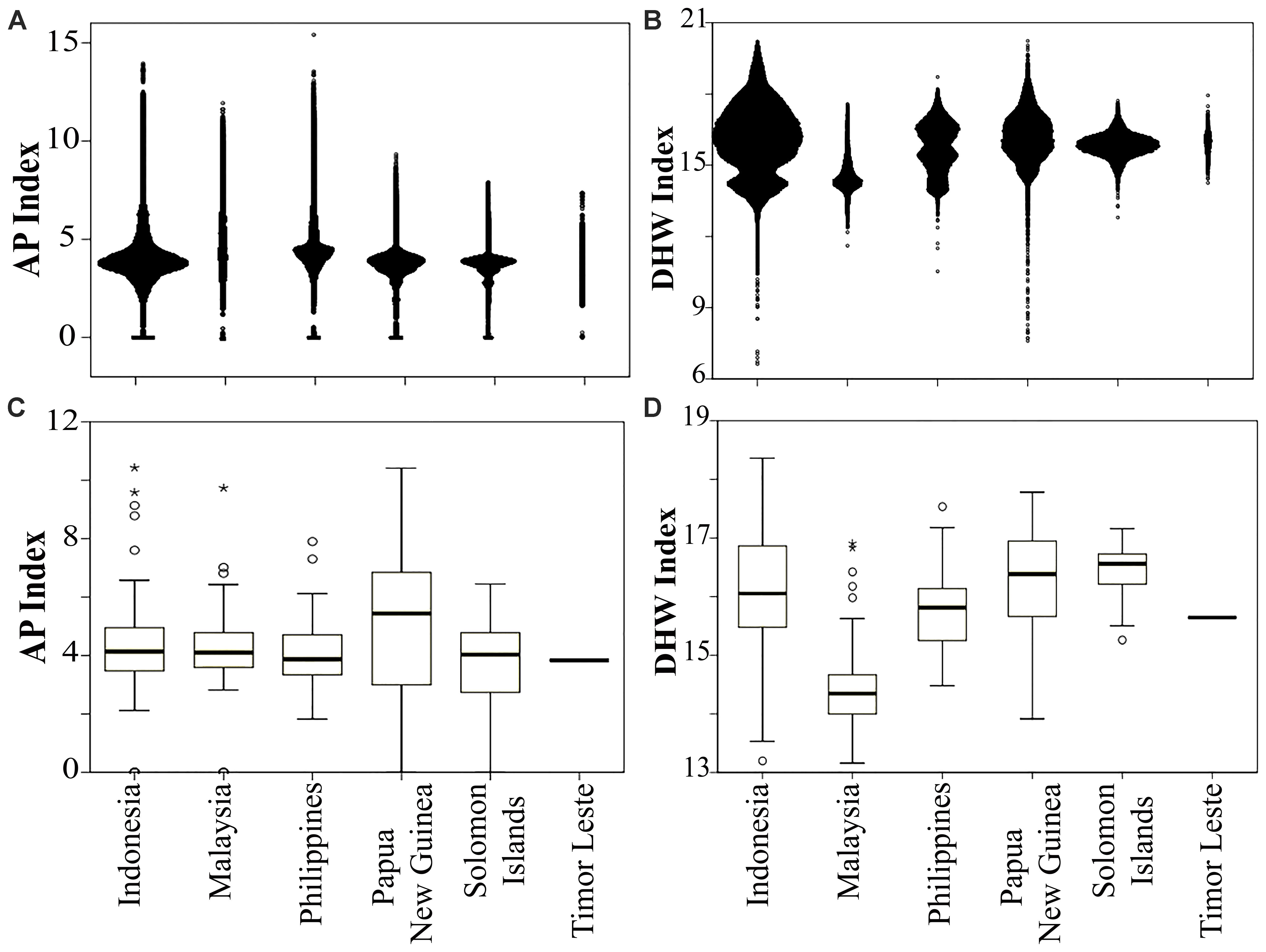
FIGURE 4. Distribution of anthropogenic pressure (AP) in panel (A) each country and (C) within MPAs (n = 678), and thermal stress (DHW) in panel (B) each country and (D) within MPAs. Timor Leste had only one MPA. Open circle and asterisk denote mild and extreme outliers, respectively.

For the projected thermal stress index (DHW), nearly 16% of the CT was categorized as low vulnerability with DHW < 14.8. These areas were found in the South China Sea, Karimata Strait, the northern part of Halmahera, the northern part of Makassar Strait, the Banda Sea, and the Gulf of Papua. High vulnerability areas with DHW > 17.2 were distributed in over 14% of the CT, predominantly in the southern part of Java and the Lesser Sunda Islands (bordering the Indian Ocean), the Java Sea, and the Bismarck Sea (bordering the Pacific Ocean) (Figures 3B, 4B).

Of 678 MPAs analyzed in this study, 22% had a medium (AP 3.1–4.8), and 41% had a high vulnerability to anthropogenic pressure (AP > 4.8). On average, Papua New Guinea’s MPAs had the lowest, while the Philippines’ MPAs had the highest AP index. The MPA which had the highest AP index in the CT is the 45 ha Pulau Rambut Wildlife Reserve, a designated international Ramsar site located 10 km to the north of Jakarta, the capital of Indonesia (Figure 4C and Supplementary Table S2).

A large proportion of the MPAs (76%) had a medium thermal stress index (DHW range: 14.8–17.2), while about 10% were ranked as having a high vulnerability to climate warming. On average, the Philippines MPAs were the most vulnerable to thermal stress, while Malaysian MPAs were the least. More than 13% of the Philippines MPAs were predicted to experience a high DHW index. The highest DHW was identified in the Pulau Noko, and Nusa Nature Reserve, a protected area in the Java Sea, and the lowest was in the Pulau Seri Buat and Pulau Sembilang Parks (part of Tioman Marine Park), located off the north coast of the Malaysian peninsula (Figure 4D and Supplementary Table S2).

Biodiversity Prioritization

(a) Analysis of the “Biodiversity-Optimized” and “Existing-Protection” Scenarios

The “Biodiversity-optimized” analysis indicated that, as expected, the average representation of biodiversity features increased in parallel with increasing extent of protection. In particular, by increasing the extent of protection from the current 1.8–10%, 20%, or 30% of CT area, the average representation across all features was increased from about 14–44%, 59%, or 70%, respectively (Figure 5). However, the conservation performance curve (i.e., a line graph consisting of the extent of protection plotted against biodiversity feature representation) was variable for each feature. The habitat rugosity feature increased nearly linearly in representation as MPA coverage increased, while other features displayed more asymmetric curves (Supplementary Figure S1b).

FIGURE 5

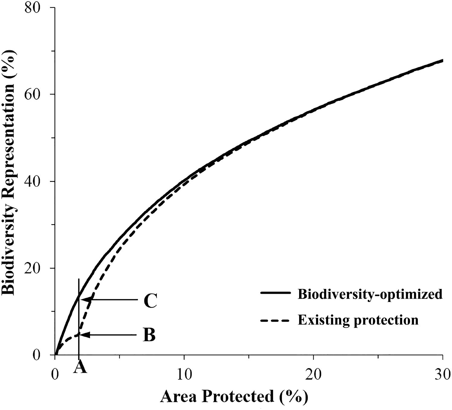
FIGURE 5. Average representation of biodiversity features within the existing (dashed line), and proposed expanded MPA network designed using Zonation (solid line). (A) Existing coverage of MPA system (1.8%); (B) average biodiversity features protected within existing MPAs (5.2%); (C) potential biodiversity features protected (13.7%) in expanded MPA system.

The “Existing Protection” analysis showed that the average representation of biodiversity features protected within the existing MPA system (i.e., the 1.8% of the CT’s EEZ) was about 5%. The biogenic habitat had the highest representation in protected areas at over 12% and was the only biodiversity feature that had achieved the CBD Aichi target of 10% protection (Figure 6 and Supplementary Figure S1a).

FIGURE 6

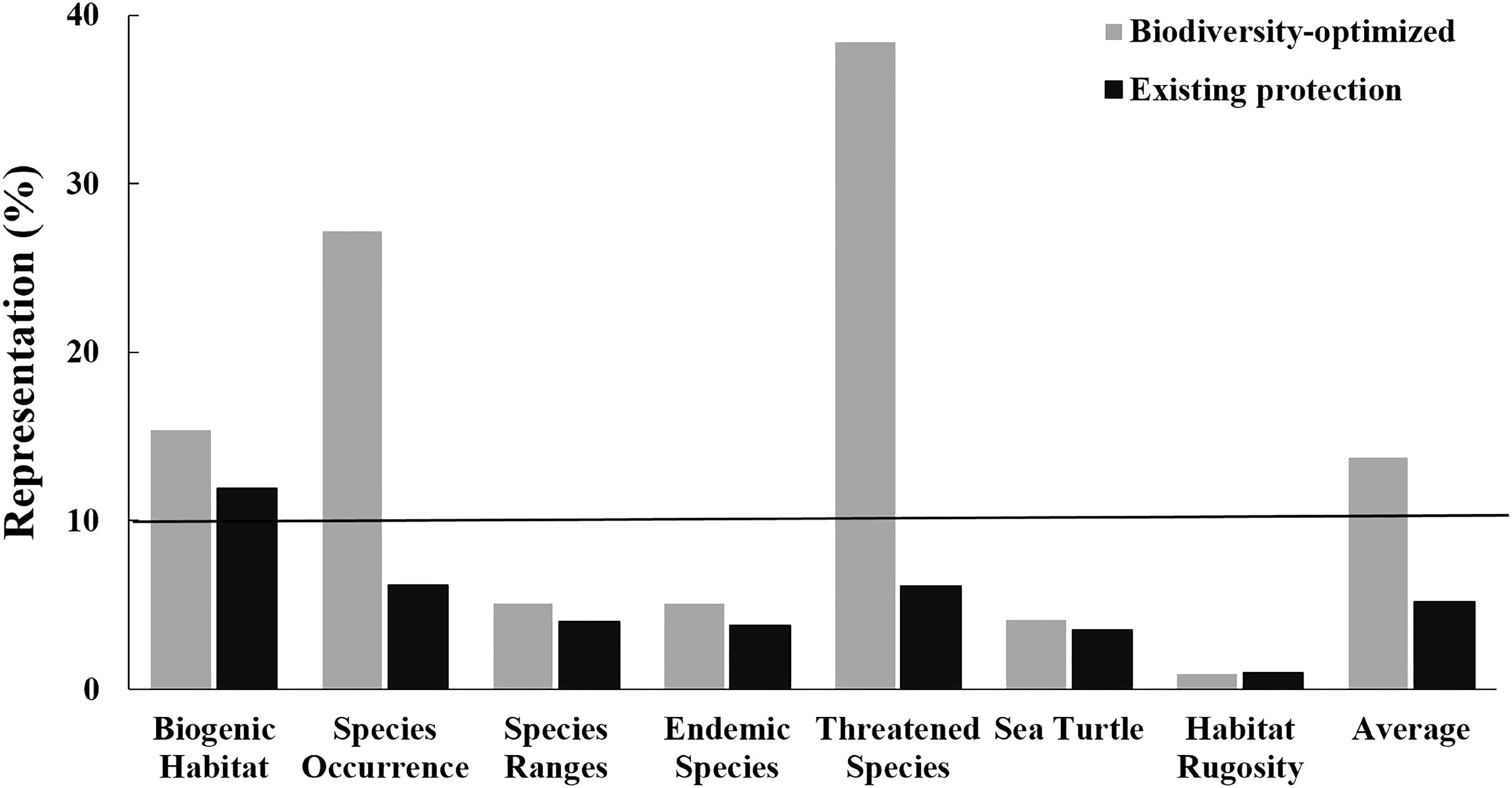
FIGURE 6. Representation of biodiversity features within the existing CT MPA system (black bars; the “existing Protection”) and an MPA network of an equivalent area but optimally designed using the systematic conservation planning tool Zonation (gray bars; the “Biodiversity-optimized scenario”). Black line indicates 10% of biodiversity features represented.

Importantly, for an area equivalent to the existing MPA system (i.e., 1.8% of the CT’s EEZ), an MPA system designed using the “Biodiversity-optimized” analysis would provide, on average, protection of nearly 14% of the biodiversity features analyzed. Under this optimized scenario, even with only 1.8% of the CT EEZ within MPA, three features would gain a protection of more than 10% (i.e., biogenic habitat, species occurrence, and threatened species) (Figure 6).

(b) “Threat” Analysis

Regional analysis

The “Threat” analysis indicated the spatial distribution of new and expanded MPAs if the CT countries opted to collaboratively expand the current CT MPA system from 1.8 to 10%, 20%, or 30% of their combined EEZ areas, while incorporating vulnerability to threats to avoid areas with high levels of anthropogenic and climate-related threats that result in decreased long-term resilience. This analysis showed that by systematically increasing the biodiversity protection of the CT MPA system to 10%, the average representation of biodiversity features within the MPA system could increase to over 37%. In the 10% scenario, the distribution of three biodiversity features (biogenic habitat, species richness-occurrence, and threatened species) could be protected by more than 60%. Using the scenario of expansion to cover 30% of the CT EEZ’s, the analysis showed the average representation of biodiversity features within the MPA system would be over 65% with each of the biodiversity features examined protected by more than 45% (except for habitat rugosity) (Figure 7). These analyses selected areas with minimal overlap with the anthropogenic and climate-induced threat layers, reducing the potential efficiency of selected MPAs for biodiversity protection (e.g., decreased average biodiversity protection from 44 to 37% within the top 10% prioritized area). For some APs, these spatial differences can be interpreted as avoidance of high conflict areas of resource extraction or other human-induced pressures which are often associated with habitat degradation that reduces biodiversity value.

FIGURE 7

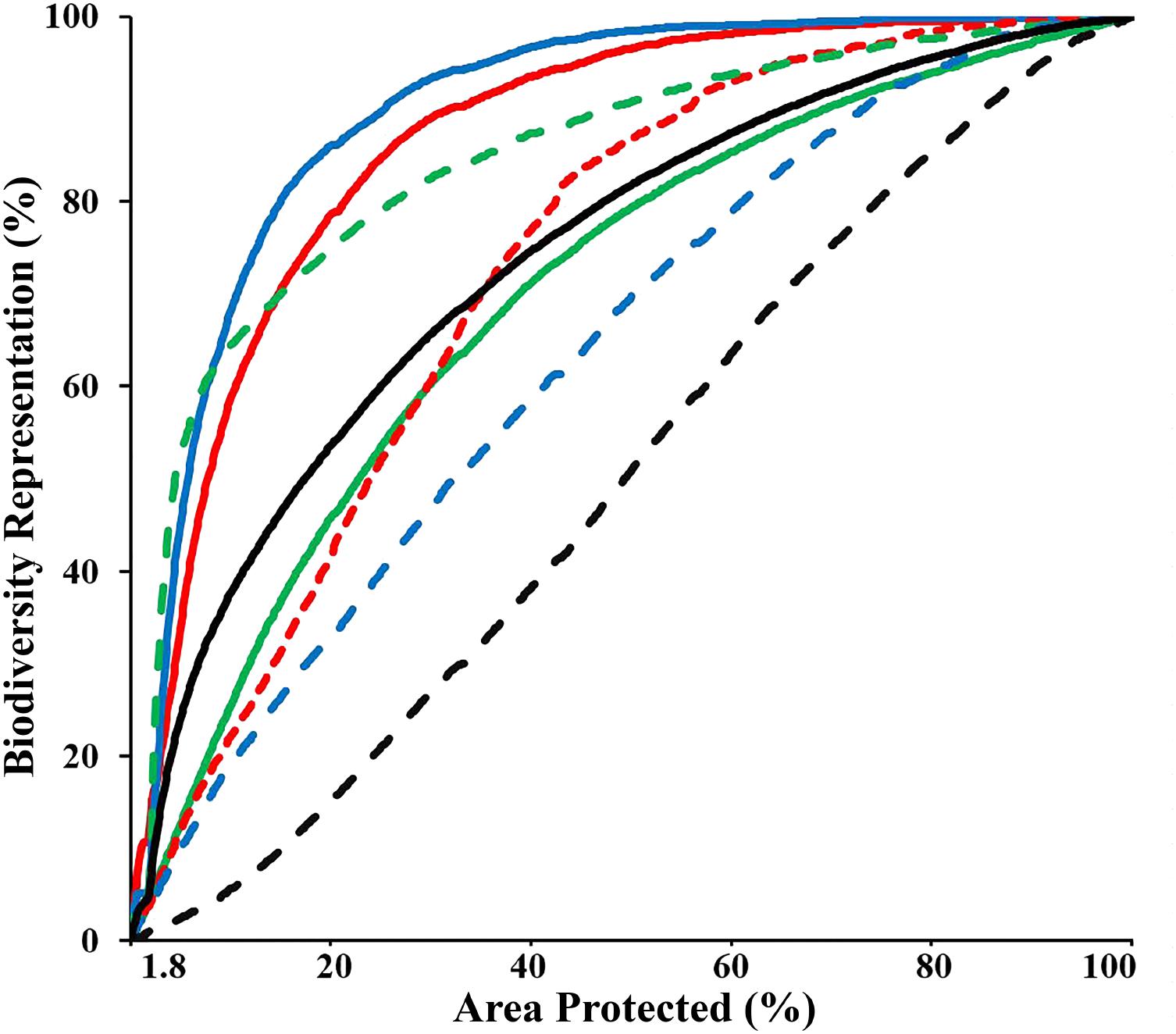
FIGURE 7. Performance curves of the biodiversity features, which describe the coverage of biodiversity representation as a function of area under protection, based on the “Threat analysis” to the full CT EEZ. Lines colors indicate: biogenic habitat (solid red); species-richness occurrence (solid blue); species-richness ranges (solid green); restricted range species (dashed red); threatened species (dashed green); areas important for sea turtles (dashed blue); habitat rugosity (dashed black); Average of all biodiversity features (solid black).

Based on the 10% scenario in the regional analysis, the Philippines would protect over 12% of its EEZ but the Solomon Islands just 1.8%. Using the 30% scenario, all of the CT countries would protect their EEZ by more than 10%. The Philippines and Timor Leste would protect over 42 and 46% of their EEZ, respectively (Table 2 and Figures 8A–C).

TABLE 2

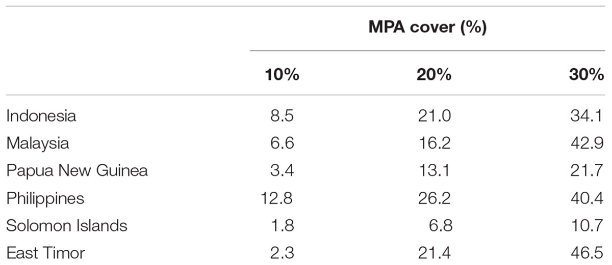
TABLE 2. Proportions of priority areas falling within each CT country’s EEZ based on the “Threat analysis” to the full CT EEZ region.

FIGURE 8

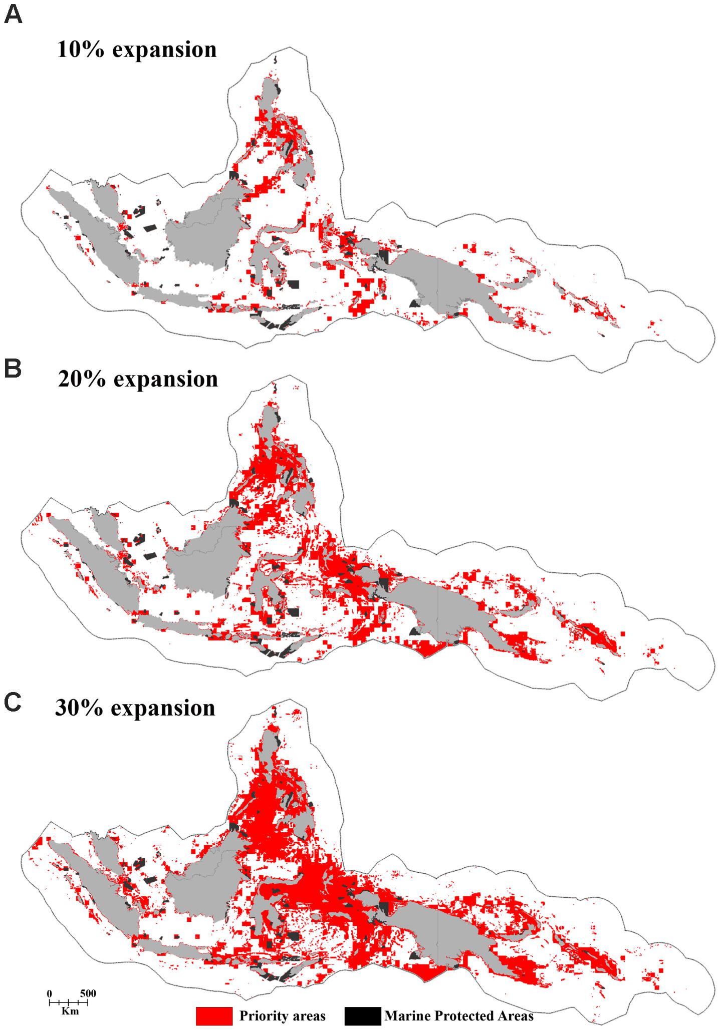
FIGURE 8. The distribution of priority areas for the potential MPA network based on the “Threat analysis” of the full CT EEZ region for the panels (A) 10%, (B) 20%, and (C) 30% MPA coverage expansion scenarios.

The regional priorities for expanded protection (i.e., the top 10% highest priority areas identified in the regional “Threat” analysis) include marine areas in the central part of the Philippines, a region stretching from Halmahera to the Birds Head Peninsula of Papua, the outer island arc of the Banda Sea in Indonesia, the north-eastern part of Sabah-Malaysia, Milne Bay Province in Papua New Guinea, and the Malaita region in the Solomon Islands (Figure 8A).

National analysis

The “Threat” analysis was also performed at the national level by expanding from the existing MPA system to 10%, 20%, or 30% of each CT country’s EEZ. Using the 10% scenario, the average proportions of biodiversity features protected in each CT country ranged from 38 to 49%. The highest biodiversity protection was ascribed to the Solomon Islands while the smallest was for Timor Leste (Figure 9).

FIGURE 9

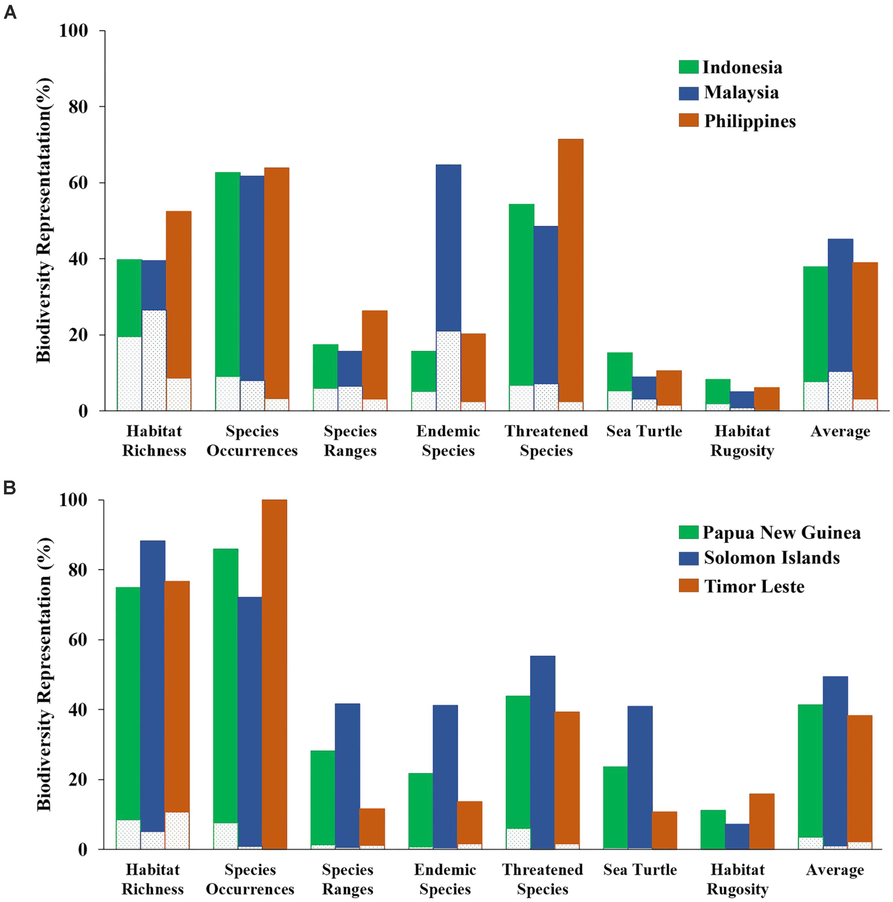
FIGURE 9. Representation of biodiversity features based on the “Threat analysis” for each of the national EEZs with 10% coverage scenario: (A) Indonesia, Malaysia, and the Philippines; (B) Papua New Guinea, Solomon Islands, and Timor Leste. Dashed portion of bars indicates biodiversity representation within existing MPA system. Solid portion of bars indicates biodiversity representation within proposed 10% coverage scenario.

The highest priority areas for enhanced protection (i.e., the top 10% highest priorities) were identified in Indonesia (e.g., in the Halmahera Sea, the Banda Sea, the Sulawesi Sea, the Makassar Strait, Lesser Sunda, and the Bird’s Head of Papua), the Philippines (e.g., the Sulu archipelago, the Bohol Sea, and the Visayan Sea), Malaysia (e.g., Sabah, and Johor), Papua New Guinea (e.g., the Bismarck Archipelago, and Milne Bay), and in the Solomon Islands (e.g., Malaita and San Cristóbal Island) (Figures 10A–F).

FIGURE 10

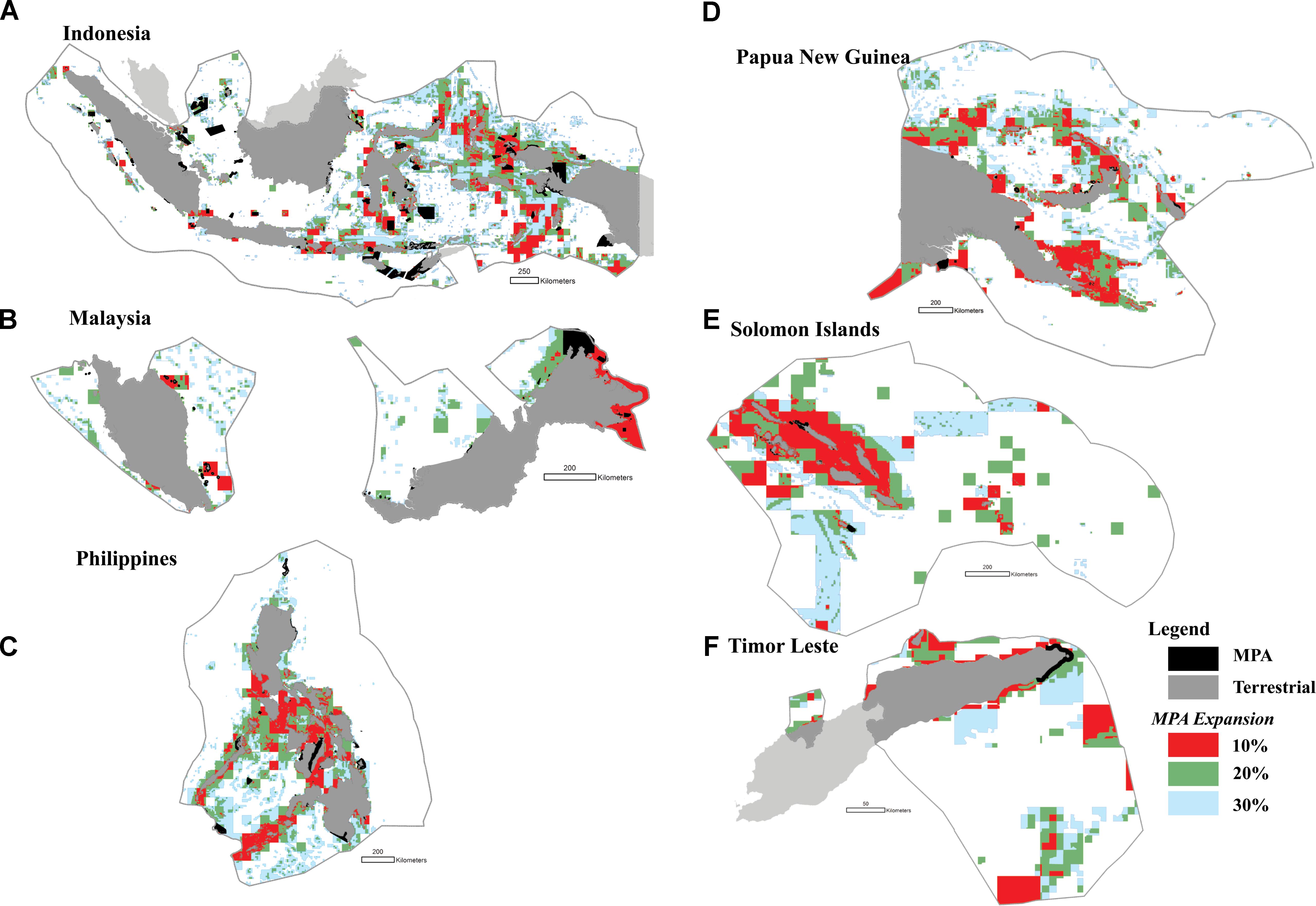
FIGURE 10. The distribution of priority areas for MPAs in each of the six CT countries based on the seven biodiversity features and threats; (A) Indonesia; (B) Malaysia; (C) The Philippines; (D) Papua New Guinea; (E) Solomon Islands; (F) Timor Leste. Colors show existing MPA coverage (black), and proposed 10% (red), 20% (green), and 30% (light blue) MPA coverage.

In addition, we found that several MPAs should optimally be expanded to cover adjacent biodiversity features, including marine parks in Indonesia (e.g., Taka Bonerate National Park, Togean, Kepulauan Seribu, Bunaken, Komodo, and MPAs in the Birds Head of Papua), the Philippines (e.g., MPAs in the northwestern part of the Sibuyan Sea, the Visayan Sea, and the Bohol Sea), Malaysia (e.g., MPAs in the northern and eastern part of Sabah), Papua New Guinea (e.g., MPAs in Madang, and Milne Bay), and the Solomon Islands (e.g., MPAs in Santa Isabel Island) (Figures 10A–F).

Discussion

Our analysis identified locations where MPAs would optimally be designated to represent the range of biodiversity in the CT (Figures 8, 10). Our regional analysis showed that by increasing the coverage of the MPA system to 10% of the CT EEZs, the average representation of biodiversity features that could be protected would increase to over 37%, even when priorities are selected to minimize overlap with high levels of threats to biodiversity. Furthermore, our national analysis also identified locations in the CT that could be optimally delineated as new MPAs to protect biodiversity (e.g., Halmahera region in Indonesia), and MPAs that could be extended to cover important biodiversity features in their adjacent waters (e.g., MPA in the Sulu Archipelago of the Philippines).

The CBD Aichi Target No. 11 calls for 10% of the ocean to be protected within MPAs, and the recent IUCN congress called for 30% in fully protected (i.e., no-take) MPAs (World Conservation Congress, 2016). There is no scientific consensus that protecting 10% of the ocean would be sufficient to protect all habitats and species, especially if the 10% is not full protection (Costello and Ballantine, 2015). Our data confirm this. First, if designed for the same 1.8% area coverage, the present CT MPA system could have protected three times more biodiversity. Because there is no reason to think that other MPA networks would have been optimally designed, then simply increasing current MPA cover to arbitrary percent targets is unlikely to ensure adequate protection of biodiversity. Even using spatial prioritization analysis to map an ideal MPA system, we find that fully protecting 10% would only protect about half of the biodiversity features. However, following the IUCN congress recommendation, 30% cover by MPAs could represent protection of 65% of the biodiversity features.

Gap Analysis of Threats

We applied two types of threats to biodiversity conservation: anthropogenic and climate change-induced stressors. Our analysis found that half of the CT was categorized as areas which had high vulnerability to present APs. These areas are mainly located adjacent to highly populated regions or to a major economic hub of the region where development is expanding significantly. Examples of high stress areas include the Malacca Strait and the South China Sea (known as the world’s main shipping lane connecting the Indian Ocean to the Pacific Ocean), and the Java Sea (one of the main fishing areas for Indonesia, with almost 70% of its fisheries stocks considered to be over-exploited) (MOMAF, 2016b).

Nearly 41% of the existing CT MPAs are categorized as highly vulnerable to APs, while 10% of the MPAs were projected to have a high vulnerability to thermal stress over the next century. Knowledge of MPA threat levels provides key information for developing alternative management strategies. MPAs which have a high vulnerability to both anthropogenic and climate change pressure should be prioritized and reinforced with strategies to reduce human impacts, such as fisheries enforcement and management (McLeod et al., 2010), habitat restoration programs (Maynard et al., 2015; Harris et al., 2017), and climate change mitigation actions including reef recovery strategies (McLeod et al., 2009; Green et al., 2014). Conversely, MPAs with low vulnerabilities to both anthropogenic and climate change pressure should be prioritized as climate change refugia and possibly as candidates for MPA expansion (McLeod et al., 2010; Harris et al., 2017). MPA management plans should, moreover, be integrated within a broader framework of marine spatial planning and other ecosystem-based management regimes to effectively control negative impacts of upstream development (Hiscock, 2014; Mills et al., 2015).

Spatial Prioritizations

Our analysis shows the advantage of applying a systematic spatial prioritization tool to identify representative areas for biodiversity conservation. With coverage equal to the existing MPA system (i.e., 1.8% of the EEZs), the “Biodiversity-optimized” analysis was able to represent almost three times more biodiversity compared to the existing MPA system (i.e., the “Existing Protection” analysis) (Figure 6). The “Existing Protection” analysis also showed that the extent of the existing MPA system had limited overlap with the areas of highest biodiversity, and is thus not optimizing protection of biodiversity. Under this Existing Protection scenario, only the “biogenic habitats” feature achieved a representation of over 10% protection in the MPA system. Importantly, using the systematic “Biodiversity-optimized” analysis, we showed that, even with an optimized design, 1.8% coverage of the CT EEZ area is still insufficient to properly protect all important biodiversity features in the region – with 4 out of 7 of the biodiversity features we analyzed (i.e., species ranges, endemic species, areas important for sea turtle, and habitat rugosity) having less than 10% representation within the optimized MPA system at 1.8% spatial coverage. If the CT countries are to achieve the CBD – Aichi Biodiversity Target 11, they will need to increase the spatial coverage of the CT MPA network significantly. Our analyses indicate that targets of 10% of the oceans will be more successful to conserve biodiversity if they are designed systematically to protect habitats and species, as a poorly selected 10% could lead to very low biodiversity protection and limited representativeness.

The “Threat” analysis identified areas within which to expand the MPA system to represent more biodiversity, and include primarily areas that had a lower vulnerability to anthropogenic and climate pressures. We analyzed expansion scenarios at both the regional (i.e., the full CT EEZ region) and national levels (i.e., for each of the CT country EEZs). With a 10% regional expansion scenario, we identified the following areas as the top priorities for designation of new MPAs: the Halmahera Sea and outer Banda Arc in Indonesia, the Sulu archipelago in the Philippines, north-eastern Sabah in Malaysia, Milne Bay in Papua New Guinea, and Malaita Island in the Solomon Islands. Our national-level analysis identified similar priorities, though with additional recommendations for MPA expansion as detailed in the results section above. Importantly, the top priorities for MPA expansion in the CT identified in our analysis have also been identified in previous national prioritization efforts. For instance, national gap assessments of MPA coverage in Indonesia (MoF-MoMAF, 2010; Huffard et al., 2012) identified the Halmahera ecoregion as an area in urgent need of conservation efforts, given its extremely high biodiversity with no MPA in place to protect its biodiversity. Similarly, the Sulu Archipelago in the Philippines was identified by Ambal et al. (2012) as a top priority for MPA expansion, yet it has only a few small community-based MPAs in place.

The national analysis provides a set of spatial priorities to assist each CT country to individually achieve their CBD Aichi Biodiversity Target No. 11, through selection of optimal and efficient representative areas that protect biodiversity rather than ad hoc and less efficient selection of MPAs (Stewart et al., 2003). These spatial priorities include both areas that should be considered for inclusion in new MPAs as well as those that are adjacent to existing MPAs and which could be included in an expansion of those MPAs. The analysis also shows that relatively small strategic increases in the overall geographic extent of Existing Protection results in rapid increases in the representation of the selected biodiversity features. By increasing their MPA system coverage to 10%, the average proportion of biodiversity features that could be protected by each CT country was over 35%. Coastal biogenic habitat was one feature that could be protected extensively by each country with smallest increasing in MPA coverage. Each CT country could protect more than 55% of their biogenic habitat by increasing their MPA system to 10% full protection (Figures 9, 10). These analyses show results for average biodiversity protection across the CT region; regional and national priorities for protection of particular features (e.g., endemic or threatened species) may vary, and our approach can be modified to include variation in conservation requirements based on both local differences in biodiversity priorities, and differences in biological requirements for individual features to suit life history strategies.

Our analysis did not include a number of potential options within the Zonation software to account for connectivity between biodiversity features, ranging from simpler options such as the “boundary length penalty” which decreases fragmentation of prioritized locations through minimizing the perimeter of protected areas, to more complex connectivity algorithms such as the “boundary quality penalty” which allows input of feature-specific connectivity parameters to allow inclusion of species- or habitat-specific responses to habitat fragmentation (Moilanen et al., 2009). Unfortunately, connectivity parameters are not available for the majority of the ∼20,000 species and habitats that we included in our CT regional model, not an uncommon issue for spatial planning (Berkström et al., 2012) (though note Green et al., 2015 have estimated connectivity patterns of 210 coral reef fishes, including many found in the CT). Our approach, in contrast, was to include connectivity more implicitly, assuming that at the scale of our analyses, each cell likely includes a habitat mosaic of different reef types as well as connectivity between reefs and other coastal habitats, as is recognized to support life history strategies of many fish (Nagelkerken et al., 2015). Elsewhere, conservation prioritizations have included data on connectivity of 288 Mediterranean fish species, illustrating that optimal conservation benefits occur when incorporating both connectivity and representativeness (Magris et al., 2018). As more complete information becomes available for CT biodiversity, future spatial planning scenarios for the CT can include connectivity and other ecological parameters, for example, more complex predictions of the implications of climate change on species range shifts and habitat suitability (Edwards et al., 2010; Jones et al., 2016; Álvarez-Romero et al., 2018).

A representative set of biodiversity datasets is needed to expedite the process of delineating areas of biodiversity importance (Roberts et al., 2003a; Gilman et al., 2011; Clark et al., 2014; Eken et al., 2016). Based on available biological data, this study performed analyses using five out of eight recommended ecological criteria (Asaad et al., 2016). Although the analysis was successfully performed and did identify areas of biodiversity importance, adding more biodiversity datasets to the analysis may generate alternative options. Our study had maps of distinct shallow-water biogenic habitats (mangroves, seagrass, and coral reef) that are key for ecological integrity, and would encompass areas of sediment and rocky substrata. Future work is needed to develop a more complete habitat map and classification system for the CT to assess the conservation priorities for other intertidal, subtidal, and deep-sea habitats.

The use of coastal biogenic habitats (coral reefs, seagrass, and mangroves) as a criterion to prioritize areas for biodiversity conservation may bias toward specific areas (Briscoe et al., 2016) and species (Ban, 2009). Sampling efforts are generally biased toward these habitats, possibly skewing their importance relative to other habitats, e.g., soft sediments or rocky shore (Jackson and Lundquist, 2016). This study used a benthic rugosity index as a surrogate for the lack of information on the distributions of different soft sediment habitats. Elsewhere, rugosity is regularly included in the delineation of benthic habitats, including soft sediment habitats (e.g., Pitcher et al., 2012). In the absence of other data, this proxy for habitat heterogeneity using benthic terrain rugosity and topographic ruggedness can be derived from bathymetric data that is available at a global scale. However, detailed habitat maps and a defined list of habitats (beyond the three for which distribution data were available) would be preferable to develop a comprehensive biodiversity prioritization, as bathymetry and slope are not the only drivers of habitat heterogeneity in most soft sediment habitats (Leathwick et al., 2006; Hewitt et al., 2015).

A precautionary approach should be considered with regard to spatial planning and governance to minimize human impacts (Appeldoorn, 2008). In the face of uncertainty, this study applied data redundancy to ensure that areas with similar biodiversity features were protected. Thus, areas with high rugosity and/or several biogenic habitats tend to have high species richness and high species endemicity. Here, the climate change pressure data was applied in both the historical (Halpern B. et al., 2015; Halpern B.S. et al., 2015) and projected data (van Hooidonk et al., 2016). In addition, the analyzed species ranges and distribution datasets account for a wide range of marine species, from common to protected and endemic species. Addressing redundancy may benefit as an insurance policy for environmental change to allow for adaptive management (Foley et al., 2010; Metcalfe et al., 2017). Our analyses are solely based on ecological criteria and are focused primarily on including a full range of biodiversity features and on ensuring the protection of ecologically significant areas. If alternative locations for expansion are identified due to political or other reasons, they will need to be larger than the areas proposed here to provide the same protection of biodiversity. Such options are of course possible and may be preferred when other factors important in MPA site selection and management are considered. These factors may include social, cultural, religious, philosophical, political, and economic (e.g., tourism and fisheries) perspectives. Such factors will need to be considered by the local and national authorities in each of the CT countries in implementing more sustainable use and conservation of marine biodiversity in the region. The present study provides objective scientific evidence to underpin such planning.

Socioeconomic and political considerations may drive processes for identifying potential MPA sites, and may have a strong influence in selecting criteria to identify areas of importance for biodiversity conservation (Roberts et al., 2003b; Gilman et al., 2011). Importantly, the conservation planning tools utilized in this study rely heavily on spatial data, making them generally much better suited for application to ecological criteria than to socio-economic or governance parameters which are often comprised of non-spatial data. Lundquist and Granek (2005) highlighted the criterion of stakeholder involvement during the process of design and implementation as a key characteristic of successful marine conservation strategies, while Gilman et al. (2011) synthesized an exhaustive list of socioeconomic and governance criteria, such as sustainable financing, legal and management frameworks, resources for management, surveillance and enforcement, and compatible existing uses which are mostly in the form of non-spatial data. Later, Mangubhai et al. (2015) proposed an alternative approach by combining analysis of ecological and spatial socioeconomic datasets such as land and sea tenure, subsistence and artisanal fishing grounds, and community designed zoning plans using decision support tools. Thus, collating and incorporating social aspect into geographic prioritization scenario may generate an environmental stewardship of communities that may lead to social acceptability and awareness to support the siting and implementation of MPAs.

Conclusion

Our analysis used biodiversity variables that captured significant biodiversity values based on habitat and species specific attributes. Systematically combining all these biodiversity datasets provided representative information upon which to prioritize areas for biodiversity conservation. We incorporated matrices of threats to account for a rapid increase in the intensity of human activities and the impact of climate change on the marine environments. We used spatial conservation prioritization tools to ensure representation of biodiversity features while minimizing costs associated with biodiversity threats. Almost all of the datasets and analysis tools were retrieved from publicly available sources to show conclusively that the application of marine biodiversity informatics supports conservation prioritization. Finally, our case study of the CT demonstrated how to develop a set of spatial priorities for biodiversity conservation simultaneously at both the regional and national scale. This approach is also readily replicated in other regions and countries to achieve a global representation of MPAs.

This study has demonstrated that the application of systematic design tools, instead of ad hoc approaches, can support the design of comprehensive MPA system by optimizing the protection of a representative range of biodiversity. Our analysis shows that, with an equivalent area, the application of evidence-based MPA design tools provides almost three times more representation of biodiversity features than that currently provided by the existing MPA system in the CT. Furthermore, the application of spatial decision support tools assisted in identifying a set of priority areas that may support designation of new MPAs and MPA expansions by extending the coverage of existing MPAs to adjacent areas in order to comprehensively protect additional important biodiversity features. This assessment will assist CT countries in optimizing their conservation investment where conservation actions will deliver the most effective conservation impact in the least area, and provide a scheme to fulfill their obligations to achieve the CBD-Aichi Biodiversity Target 11 and the United Nation-Sustainable Development Goals 14.

The present study demonstrates how other geographic regions could similarly collate data from OBIS, GBIF and other sources to systematically design an MPA system that optimizes conservation of all aspects of biodiversity. Our finding that one third of the area can represent two-thirds of the biodiversity merits testing in other regions. If found to be a useful general rule for large geographic areas, it provides an objective basis that supports the IUCN call for 30% of the ocean to be in fully protected, no fishing, MPA.

Author Contributions

IA conceived and conducted the literature review, collated the data, analyzed the data, wrote the paper, prepared the figures and tables, and reviewed drafts of the paper. CL, ME, RVH, and MC provided guidance and reviewed drafts of the paper.

Funding

IA was supported by New Zealand Aid Programme through New Zealand – ASEAN Scholarship.

Conflict of Interest Statement

The authors declare that the research was conducted in the absence of any commercial or financial relationships that could be construed as a potential conflict of interest.

Acknowledgments

We would like to thank Dr. Maria Beger and Ruben Venegas Li for their insightful input into earlier conceptualizations of this research.

Supplementary Material

The Supplementary Material for this article can be found online at: https://www.frontiersin.org/articles/10.3389/fmars.2018.00400/full#supplementary-material

FIGURE S1 | Performance curves of the biodiversity features, which describe the coverage of biodiversity representation as a function of area under protection, based on the (a) “existing analysis”; (b) “Biodiversity-optimized” to the full Coral Triangle EEZ. Lines colors indicate: biogenic habitat (solid red); species-richness occurrence (solid blue); species-richness ranges (solid green); restricted range species (dashed red); threatened species (dashed green); areas important for sea turtles (dashed blue); habitat rugosity (dashed black); Average of all biodiversity features (solid black).

TABLE S1 | List of marine protected areas in the Coral Triangle (n = 678).

TABLE S2 | Mean value of the anthropogenic pressure (AP Index) and he projected thermal stress (DHW Index) within each MPA in the Coral Triangle.

Footnotes

1. ^ www.protectedplanet.net
2. ^ ctatlas.reefbase.org

References

Allen, G. R. (2008). Conservation hotspots of biodiversity and endemism for Indo-Pacific coral reef fishes. Aquat. Conser. 18, 541–556. doi: 10.1002/Aqc.880

CrossRef Full Text | Google Scholar

Allen, G. R., and Erdmann, M. V. (2013). Reef Fishes of the East Indies. Mobile Application Software. Version 1.1 (Rev.10.2016). Available at: https://geo.itunes.apple.com/us/app/reef-fishes-east-indies-vol./id705188551?mt=8 [accessed June 15, 2016].

Google Scholar

Álvarez-Romero, J. G., Munguía-Vega, A., Beger, M., Mar Mancha-Cisneros, M., Suárez-Castillo, A. N., Gurney, G. G., et al. (2018). Designing connected marine reserves in the face of global warming. Glob. Change Biol. 24, e671–e691. doi: 10.1111/gcb.13989

PubMed Abstract | CrossRef Full Text | Google Scholar

Ambal, R., Duya, M., Cruz, M., Coroza, O., Vergara, S., De Silva, N., et al. (2012). Key biodiversity areas in the Philippines: priorities for conservation. J. Threat. Taxa 4, 2788–2796. doi: 10.1371/journal.pone.0029080

PubMed Abstract | CrossRef Full Text | Google Scholar

Anthony, K., Marshall, P. A., Abdulla, A., Beeden, R., Bergh, C., Black, R., et al. (2015). Operationalizing resilience for adaptive coral reef management under global environmental change. Glob. Change Biol. 21, 48–61. doi: 10.1111/gcb.12700

PubMed Abstract | CrossRef Full Text | Google Scholar

Appeldoorn, R. S. (2008). Transforming reef fisheries management: application of an ecosystem-based approach in the USA Caribbean. Environ. Conserv. 35, 232–241. doi: 10.1017/S0376892908005018

CrossRef Full Text | Google Scholar

Asaad, I., Lundquist, C. J., Erdmann, M. V., and Costello, M. J. (2016). Ecological criteria to identify areas for biodiversity conservation. Biol. Conserv. 213, 309–316. doi: 10.1016/j.biocon.2016.10.007

CrossRef Full Text | Google Scholar

Asaad, I., Lundquist, C. J., Erdmann, M. V., and Costello, M. J. (2018). Delineating priority areas for marine biodiversity conservation in the Coral Triangle. Biol. Conserv. 222, 198–211. doi: 10.1016/j.biocon.2018.03.037

PubMed Abstract | CrossRef Full Text | Google Scholar

Ball, I. R., Possingham, H. P., and Watts, M. (2009). “Marxan and relatives: software for spatial conservation prioritisation,” in Spatial Conservation Prioritisation: Quantitative Methods and Computational tools, eds A. Moilanen, K. A. Wilson, and H. Possingham (Oxford: Oxford University Press), 185–195.

Google Scholar

Ban, N. C. (2009). Minimum data requirements for designing a set of marine protected areas, using commonly available abiotic and biotic datasets. Biodivers. Conserv. 18, 1829–1845. doi: 10.1007/s10531-008-9560-8

CrossRef Full Text | Google Scholar

Barnosky, A. D., Matzke, N., Tomiya, S., Wogan, G. O., Swartz, B., Quental, T. B., et al. (2011). Has the Earth’s sixth mass extinction already arrived? Nature 471, 51–57. doi: 10.1038/nature09678

PubMed Abstract | CrossRef Full Text | Google Scholar

Basher, Z., Bowden, D. A., and Costello, M. J. (2014). Global Marine Environment Datasets (GMED)- World Wide Web Electronic Publication. Version 1.0 (Rev.01.2014). Available at: http://gmed.auckland.ac.nz [accessed June 01, 2014]

Google Scholar

Beger, M., McGowan, J., Treml, E. A., Green, A. L., White, A. T., Wolff, N. H., et al. (2015). Integrating regional conservation priorities for multiple objectives into national policy. Nat. Commun. 6:8208. doi: 10.1038/ncomms9208

PubMed Abstract | CrossRef Full Text | Google Scholar

Beger, M. J., McGowan, S. F., Heron, E. A., Treml, A., Green, A. T., White, N. H., et al. (2013). Identifying Conservation Priority Gaps in the Coral Triangle Marine Protected Area System. Arlington County, VA: The Nature Conservancy.

Google Scholar

Berkström, C., Gullström, M., Lindborg, R., Mwandya, A. W., Yahya, S. A. S., Kautsky, N., et al. (2012). Exploring ‘knowns’ and ‘unknowns’ in tropical seascape connectivity with insights from East African coral reefs. Estuar. Coast. Shelf Sci. 107, 1–21. doi: 10.1016/j.ecss.2012.03.020

CrossRef Full Text | Google Scholar

Briscoe, D. K., Maxwell, S. M., Kudela, R., Crowder, L. B., and Croll, D. (2016). Are we missing important areas in pelagic marine conservation? Redefining conservation hotspots in the ocean. Endanger. Species Res. 29, 229–237. doi: 10.3354/esr00710

CrossRef Full Text | Google Scholar

Brooks, T. (2010). “Conservation planning and priorities,” in Conservation Biology for All, eds N. S. Sodhi and P. R. Ehrlich (Oxford: Oxford University Press), 199–217. doi: 10.1093/acprof:oso/9780199554232.003.0012

CrossRef Full Text | Google Scholar

Brooks, T. M. (2014). Conservation: mind the gaps. Nature 516, 336–337. doi: 10.1038/516336a

PubMed Abstract | CrossRef Full Text | Google Scholar

Brooks, T. M., Mittermeier, R. A., da Fonseca, G. A., Gerlach, J., Hoffmann, M., Lamoreux, J. F., et al. (2006). Global biodiversity conservation priorities. Science 313, 58–61. doi: 10.1126/science.1127609

PubMed Abstract | CrossRef Full Text | Google Scholar

Burke, L. M., Reytar, K., Spalding, M., and Perry, A. (2012). Reefs at Risk Revisited in the Coral Triangle. Washington DC: World Resources Institute.

Google Scholar

Cardinale, B. J., Duffy, J. E., Gonzalez, A., Hooper, D. U., Perrings, C., Venail, P., et al. (2012). Biodiversity loss and its impact on humanity. Nature 486, 59–67. doi: 10.1038/nature11148

PubMed Abstract | CrossRef Full Text | Google Scholar

Casey, K. S., Brandon, T. B., Cornillon, P., and Evans, R. (2010). The Past, Present, and Future of the AVHRR Pathfinder SST program oceanography from Space. London: Springer, 273–287.

Google Scholar

Clark, M. R., Rowden, A. A., Schlacher, T. A., Guinotte, J., Dunstan, P. K., Williams, A., et al. (2014). Identifying Ecologically or Biologically Significant Areas (EBSA): a systematic method and its application to seamounts in the South Pacific Ocean. Ocean Coast. Manag. 91, 65–79. doi: 10.1016/j.ocecoaman.2014.01.016

CrossRef Full Text | Google Scholar

Convention on Biological Diversity (2010). Strategic Plan for Biodiversity 2011-2020, including the Aichi Biodiversity Targets. Montreal, QC: Secretariat of the Convention on Biological Diversity.

Google Scholar

Costello, M. J., and Baker, C. S. (2011). Who eats sea meat? Expanding human consumption of marine mammals. Biol. Conserv. 144, 2745–2746. doi: 10.1016/j.biocon.2011.10.015

CrossRef Full Text | Google Scholar

Costello, M. J., and Ballantine, B. (2015). Biodiversity conservation should focus on no-take Marine Reserves: 94% of Marine Protected Areas allow fishing. Trends Ecol. Evol. 30, 507–509. doi: 10.1016/j.tree.2015.06.011

PubMed Abstract | CrossRef Full Text | Google Scholar

Costello, M. J., Cheung, A., and De Hauwere, N. (2010). Topography statistics for the surface and seabed area, volume, depth and slope, of the world’s seas, oceans and countries. Environ. Sci. Technol. 44, 8821–8828. doi: 10.1021/es1012752

PubMed Abstract | CrossRef Full Text | Google Scholar

Cros, A., Fatan, N. A., White, A., Teoh, S. J., Tan, S., Handayani, C., et al. (2014a). The coral triangle atlas: an integrated online spatial database system for improving coral reef management. PLoS One 9:e96332. doi: 10.1371/journal.pone.0096332

PubMed Abstract | CrossRef Full Text | Google Scholar

Cros, A., Venegas-Li, R., Teoh, S. J., Peterson, N., Wen, W., and Fatan, N. A. (2014b). Spatial data quality control for the coral triangle atlas. Coast. Manage. 42, 128–142. doi: 10.1080/08920753.2014.877760

CrossRef Full Text | Google Scholar

CTI-CFF (2009). The Regional Plan of Action of the Coral Triangle on Coral Reefs, Fisheries and Food Security (CTI-CFF) Initiative. Jakarta: Secretariat of CTI-CFF Initiative.

Google Scholar

CTI-CFF (2013). Coral Triangle Marine Protected Area System Framework and Action Plan. Cebu: CTI-CFFMarine Protected Area Technical Working Group and the Coral Triangle Support Partnership of USAID.

Google Scholar

Day, J. C., Roff, J., and Laughren, J. (2000). Planning for Representative Marine Protected areas: a Framework for Canada’s Oceans. Toronto: World Wildlife Fund.

Google Scholar

Donner, S. D., Skirving, W. J., Little, C. M., Oppenheimer, M., and Hoegh-Guldberg, O. (2005). Global assessment of coral bleaching and required rates of adaptation under climate change. Glob. Change Biol. 11, 2251–2265. doi: 10.1111/j.1365-2486.2005.01073.x

CrossRef Full Text | Google Scholar

Edgar, G. J., Langhammer, P. F., Allen, G., Brooks, T. M., Brodie, J., Crosse, W., et al. (2008). Key biodiversity areas as globally significant target sites for the conservation of marine biological diversity. Aquat. Conserv. 18, 969–983. doi: 10.1002/aqc.902

CrossRef Full Text | Google Scholar

Edwards, H. J., Elliott, I. A., Pressey, R. L., and Mumby, P. J. (2010). Incorporating ontogenetic dispersal, ecological processes and conservation zoning into reserve design. Biol. Conserv. 143, 457–470. doi: 10.1016/j.biocon.2009.11.013

CrossRef Full Text | Google Scholar

Eken, G., Isfendiyaroğlu, S., Yeniyurt, C., Erkol, I. L., Karataş, A., and Ataol, M. (2016). Identifying key biodiversity areas in Turkey: a multi-taxon approach. Int. J. Biodivers. Sci. Ecosyst. Serv. Manage. 12, 181–190. doi: 10.1080/21513732.2016.1182949

CrossRef Full Text | Google Scholar

ESRI (2016). ArcGIS Desktop; Release 10.5 (Vol. 2016). ESRI: Redlands, CA.

Google Scholar

Fernandes, L., Day, J., Lewis, A., Slegers, S., Kerrigan, B., Breen, D., et al. (2005). Establishing representative no-take areas in the Great Barrier Reef: large-scale implementation of theory on marine protected areas. Conserv. Biol. 19, 1733–1744. doi: 10.1111/j.1523-1739.2005.00302.x

CrossRef Full Text | Google Scholar

Foley, M. M., Halpern, B. S., Micheli, F., Armsby, M. H., Caldwell, M. R., Crain, C. M., et al. (2010). Guiding ecological principles for marine spatial planning. Mar. Policy 34, 955–966. doi: 10.1002/eap.1469

PubMed Abstract | CrossRef Full Text | Google Scholar

Froese, R., and Pauly, D. (2016). FishBase. World Wide Web Electronic Publication. Available at: www.fishbase.org. Retrieved version (06/2016)

Google Scholar

Geange, S. W., Leathwick, J., Linwood, M., Curtis, H., Duffy, C., Funnell, G., et al. (2017). Integrating conservation and economic objectives in MPA network planning: a case study from New Zealand. Biol. Conserv. 210, 136–144. doi: 10.1016/j.biocon.2017.04.011

CrossRef Full Text | Google Scholar

Gilman, E., Dunn, D., Read, A., Hyrenbach, K. D., and Warner, R. (2011). Designing criteria suites to identify discrete and networked sites of high value across manifestations of biodiversity. Biodivers. Conserv. 20, 3363–3383. doi: 10.1007/s10531-011-0116-y

CrossRef Full Text | Google Scholar

Giri, C., Ochieng, E., Tieszen, L., Zhu, Z., Singh, A., Loveland, T., et al. (2011a). Global Distribution of Mangroves Forests of the World Using Earth Observation Satellite Data. In Supplement to: Giri et al. (2011a). Cambridge: World Conservation Monitoring Centre.

Google Scholar

Giri, C., Ochieng, E., Tieszen, L., Zhu, Z., Singh, A., Loveland, T., et al. (2011b). Status and distribution of mangrove forests of the world using earth observation satellite data. Glob. Ecol. Biogeogr. 20, 154–159. doi: 10.1016/j.jenvman.2014.01.020

PubMed Abstract | CrossRef Full Text | Google Scholar

Green, A., and Mous, P. J. (2008). Delineating the Coral Triangle, its Ecoregions and Functional Seascapes TNC Coral Triangle Report. Bali: Coral Triangle Centre.

Google Scholar

Green, A. L., Fernandes, L., Almany, G., Abesamis, R., McLeod, E., Aliño, P. M., et al. (2014). Designing marine reserves for fisheries management, biodiversity conservation, and climate change adaptation. Coast. Manage. 42, 143–159. doi: 10.1080/08920753.2014.877763

CrossRef Full Text | Google Scholar

Green, A. L., Maypa, A. P., Almany, G. R., Rhodes, K. L., Weeks, R., Abesamis, R. A., et al. (2015). Larval dispersal and movement patterns of coral reef fishes, and implications for marine reserve network design. Biol. Rev. 90, 1215–1247. doi: 10.1111/brv.12155

PubMed Abstract | CrossRef Full Text | Google Scholar

Green, S. J., White, A. T., Christie, P., Kilarski, S., Meneses, A., Samonte-Tan, G., et al. (2011). Emerging marine protected area networks in the Coral Triangle: lessons and way forward. Conserv. Soc. 9, 173–188. doi: 10.4103/0972-4923.86986

CrossRef Full Text | Google Scholar

Halpern, B., Frazier, M., Potapenko, J., Casey, K., Koenig, K., Longo, C., et al. (2015). Cumulative Human Impacts: Raw Stressor Data (2008 and 2013). Available at: https://knb.ecoinformatics.org/

Google Scholar

Halpern, B. S., Frazier, M., Potapenko, J., Casey, K. S., Koenig, K., Longo, C., et al. (2015). Spatial and temporal changes in cumulative human impacts on the world/’s ocean. Nat. Commun. 6:7615. doi: 10.1038/ncomms8615

PubMed Abstract | CrossRef Full Text | Google Scholar

Halpern, B. S., Walbridge, S., Selkoe, K. A., Kappel, C. V., Micheli, F., D’Agrosa, C., et al. (2008). A global map of human impact on marine ecosystems. Science 319, 948–952. doi: 10.1126/science.1149345

PubMed Abstract | CrossRef Full Text | Google Scholar

Harris, J. L., Estradivari, E., Fox, H. E., McCarthy, O. S., and Ahmadia, G. N. (2017). Planning for the future: Incorporating global and local data to prioritize coral reef conservation. Aquat. Conserv. 27, 65–77. doi: 10.1002/aqc.2810

CrossRef Full Text | Google Scholar

Harris, P. T., and Baker, E. K. (2012). “Why map benthic habitats?,” in Seafloor Geomorphology as Benthic Habitat. Geohab Atlas of Seafloor Geomorphic Features and Benthic Habitats, eds P. T. Harris and E. K. Baker (London: Elsevier), 23–39.

Google Scholar

Heck, K. L., van Belle, G., and Simberloff, D. (1975). Explicit calculation of the rarefaction diversity measurement and the determination of sufficient sample size. Ecology 56, 1459–1461. doi: 10.2307/1934716

CrossRef Full Text | Google Scholar

Hewitt, J. E., Wang, D., Francis, M., Lundquist, C., and Duffy, C. (2015). Evaluating demersal fish richness as a surrogate for epibenthic richness in management and conservation. Divers. Distribut. 21, 901–912. doi: 10.1111/ddi.12336

CrossRef Full Text | Google Scholar

Hiscock, K. (2014). Marine Biodiversity Conservation: A practical Approach. London: Routledge. doi: 10.4324/9781315857640

CrossRef Full Text | Google Scholar

Hobson, R. (1972). “Surface roughness in topography: quantitative approach,” in Spatial Analysis in Geomorphology, ed. R. J. Chorley (London: Methue & Co), 221–245.

Google Scholar

Hooper, D. U., Adair, E. C., Cardinale, B. J., Byrnes, J. E., Hungate, B. A., Matulich, K. L., et al. (2012). A global synthesis reveals biodiversity loss as a major driver of ecosystem change. Nature 486, 105–108. doi: 10.1038/nature11118

PubMed Abstract | CrossRef Full Text | Google Scholar

Huffard, C. L., Erdmann, M. V., and Gunawan, T. R. P. (2012). Geographic Priorities for Marine Biodiversity Conservation in Indonesia. Jakarta: Ministry of Marine Affairs and Fisheries and Marine Protected Areas Governance Program.

Google Scholar

Hurlbert, S. H. (1971). The nonconcept of species diversity: a critique and alternative parameters. Ecology 52, 577–586. doi: 10.2307/1934145

PubMed Abstract | CrossRef Full Text | Google Scholar

IMARS-USF, and IRD (2005). Millennium Coral Reef Mapping Project. Validated maps. Cambridge: UNEP World Conservation Monitoring Centre.

Google Scholar

IUCN (2015). The IUCN Red List of Threatened Species. Version 2015.4. Available at: http://www.iucnredlist.org [accessed November 19, 2015]

Google Scholar

IUCN and UNEP-WCMC (2016). The World Database on Protected Areas (WDPA). Cambridge: World Conservation Monitoring Centre.

Google Scholar

Jackson, S. E., and Lundquist, C. J. (2016). Limitations of biophysical habitats as biodiversity surrogates in the Hauraki Gulf Marine Park. Pac. Conserv. Biol. 22, 159–172. doi: 10.1071/PC15050

CrossRef Full Text | Google Scholar

Jenkins, C. N., Pimm, S. L., and Joppa, L. N. (2013). Global patterns of terrestrial vertebrate diversity and conservation. Proc. Natl. Acad. Sci. U.S.A. 110, E2602–E2610. doi: 10.1073/pnas.1302251110

PubMed Abstract | CrossRef Full Text | Google Scholar

Jones, K. R., Watson, J. E. M., Possingham, H. P., and Klein, C. J. (2016). Incorporating climate change into spatial conservation prioritisation: a review. Biol. Conserv. 194, 121–130. doi: 10.1016/j.biocon.2015.12.008

CrossRef Full Text | Google Scholar

Kaschner, K., Rius-Barile, J., Kesner-Reyes, K., Garilao, C., Kullander, S. O., Rees, T., et al. (2016). AquaMaps: Predicted Range Maps for Aquatic Species. World Wide Web Electronic Publication. Available at: www.aquamaps.org.

Google Scholar

Langhammer, P. F., Bakar, M. I., Bennun, L. A., Brooks, T. M., Rob, P., Darwall, W., et al. (2007). Identification and Gap Analysis of Key Biodiversity Areas: Targets for Comprehensive Protected Area Systems. Gland: IUCN.

Google Scholar

Leathwick, J., Elith, J., Francis, M., Hastie, T., and Taylor, P. (2006). Variation in demersal fish species richness in the oceans surrounding New Zealand: an analysis using boosted regression trees. Mar. Ecol. Progr. Ser. 321, 267–281. doi: 10.3354/meps321267

CrossRef Full Text | Google Scholar

Leathwick, J., Moilanen, A., Francis, M., Elith, J., Taylor, P., Julian, K., et al. (2008). Novel methods for the design and evaluation of marine protected areas in offshore waters. Conserv. Lett. 1, 91–102. doi: 10.1111/j.1755-263X.2008.00012.x

CrossRef Full Text | Google Scholar

Lehtomäki, J., and Moilanen, A. (2013). Methods and workflow for spatial conservation prioritization using Zonation. Environ. Model. Softw. 47, 128–137. doi: 10.1016/j.envsoft.2013.05.001

CrossRef Full Text | Google Scholar

Liu, G., Strong, A. E., and Skirving, W. (2003). Remote sensing of sea surface temperatures during 2002 Barrier Reef coral bleaching. Eos Trans. Am. Geophys. Union 84, 137–141. doi: 10.1029/2003EO150001

CrossRef Full Text | Google Scholar

Lundquist, C. J., and Granek, E. F. (2005). Strategies for successful marine conservation: integrating socioeconomic, political, and scientific factors. Conserv. Biol. 19, 1771–1778. doi: 10.1111/j.1523-1739.2005.00279.x

CrossRef Full Text | Google Scholar

Magris, R. A., Andrello, M., Pressey, R. L., Mouillot, D., Dalongeville, A., Jacobi, M. N., et al. (2018). Biologically representative and well-connected marine reserves enhance biodiversity persistence in conservation planning. Conserv. Lett. 11:e12439. doi: 10.1111/conl.12439

CrossRef Full Text | Google Scholar

Magris, R. A., Pressey, R. L., Mills, M., Vila-Nova, D. A., and Floeter, S. (2017). Integrated conservation planning for coral reefs: designing conservation zones for multiple conservation objectives in spatial prioritisation. Glob. Ecol. Conserv. 11, 53–68. doi: 10.1016/j.gecco.2017.05.002

CrossRef Full Text | Google Scholar

Magris, R. A., Treml, E. A., Pressey, R. L., and Weeks, R. (2015). Integrating multiple species connectivity and habitat quality into conservation planning for coral reefs. Ecography 39, 649–664. doi: 10.1111/ecog.01507

CrossRef Full Text | Google Scholar

Mangubhai, S., Wilson, J. R., Rumetna, L., and Maturbongs, Y. (2015). Explicitly incorporating socioeconomic criteria and data into marine protected area zoning. Ocean Coast. Manage. 116, 523–529. doi: 10.1016/j.ocecoaman.2015.08.018

CrossRef Full Text | Google Scholar

Margules, C. R., and Pressey, R. L. (2000). Systematic conservation planning. Nature 405, 243–253. doi: 10.1038/35012251

PubMed Abstract | CrossRef Full Text | Google Scholar

Maynard, J. A., Mckagan, S., Raymundo, L., Johnson, S., Ahmadia, G. N., Johnston, L., et al. (2015). Assessing relative resilience potential of coral reefs to inform management. Biol. Conserv. 192, 109–119. doi: 10.1016/j.biocon.2015.09.001

CrossRef Full Text | Google Scholar

McCauley, D. J., Pinsky, M. L., Palumbi, S. R., Estes, J. A., Joyce, F. H., and Warner, R. R. (2015). Marine defaunation: animal loss in the global ocean. Science 347, 1255641. doi: 10.1126/science.1255641

PubMed Abstract | CrossRef Full Text | Google Scholar

McLeod, E., Moffitt, R., Timmermann, A., Salm, R., Menviel, L., Palmer, M. J., et al. (2010). Warming seas in the coral triangle: coral reef vulnerability and management implications. Coast. Manage. 38, 518–539. doi: 10.1080/08920753.2010.509466

CrossRef Full Text | Google Scholar

McLeod, E., Salm, R., Green, A., and Almany, J. (2009). Designing marine protected area networks to address the impacts of climate change. Front. Ecol. Environ. 7, 362–370. doi: 10.1890/070211

CrossRef Full Text | Google Scholar

Metcalfe, K., Collins, T., Abernethy, K. E., Boumba, R., Dengui, J. C., Miyalou, R., et al. (2017). Addressing uncertainty in marine resource management; combining community engagement and tracking technology to characterize human behavior. Conserv. Lett. 10, 460–469. doi: 10.1111/conl.12293

CrossRef Full Text | Google Scholar

Mills, M., Weeks, R., Pressey, R. L., Gleason, M. G., Eisma-Osorio, R.-L., Lombard, A. T., et al. (2015). Real-world progress in overcoming the challenges of adaptive spatial planning in marine protected areas. Biol. Conserv. 181, 54–63. doi: 10.1016/j.biocon.2014.10.028

CrossRef Full Text | Google Scholar

MOF-MOMAF (2010). Ecological Representation Gap Analysis for Conservation Areas in Indonesia. Jakarta: Ministry of Forestry and Ministry of Marine Affairs and Fisheries, 29.

Google Scholar

Moilanen, A. (2007). Landscape zonation, benefit functions and target-based planning: unifying reserve selection strategies. Biol. Conserv. 134, 571–579. doi: 10.1016/j.biocon.2006.09.008

CrossRef Full Text | Google Scholar

Moilanen, A., Franco, A. M., Early, R. I., Fox, R., Wintle, B., and Thomas, C. D. (2005). Prioritizing multiple-use landscapes for conservation: methods for large multi-species planning problems. Proc. R. Soc. Lond. Biol. Sci. 272, 1885–1891. doi: 10.1098/rspb.2005.3164

PubMed Abstract | CrossRef Full Text | Google Scholar

Moilanen, A., Kujala, H., and Leathwick, J. (2009). “The Zonation framework and software for conservation prioritization,” in Spatial Conservation Prioritization, eds A. Moilanen, K. A. Wilson, and H. P. Possingham (Oxford: Oxford University Press), 196–210. doi: 10.1016/j.scitotenv.2018.01.086

PubMed Abstract | CrossRef Full Text | Google Scholar

Moilanen, A., Leathwick, J. R., and Quinn, J. M. (2011). Spatial prioritization of conservation management. Conserv. Lett. 4, 383–393. doi: 10.1111/j.1755-263X.2011.00190.x

CrossRef Full Text | Google Scholar

Moilanen, A., Pouzols, F., Meller, L., Veach, V., Arponen, A., Leppänen, J., et al. (2014). Zonation–Spatial Conservation Planning Methods and Software. Version 4. User Manual. Helsinki: University of Helsinki.

Google Scholar

MOMAF (2016a). Database of Marine Protected Areas in Indonesia. Jakarta: Ministry of Marine Affairs and Fisheries.

Google Scholar

MOMAF (2016b). Ministerial Regulation No. 47/2016. Concerning on the Potential Estimations, Allowable Catch and Level of Utilization of Fisheries Resources in the Fisheries Management Areas of the Republic of Indonesia (Estimasi potensi, jumlah tangkapan yang diperbolehkan dan tingkat pemanfaataan sumberdaya Ikan di wilayah -pengelolaan perikanan negara Republik Indonesia). Jakarta: Ministry of Marine Affairs and Fisheries.

Google Scholar

Moss, R. H., Edmonds, J. A., Hibbard, K. A., Manning, M. R., Rose, S. K., Van Vuuren, D. P., et al. (2010). The next generation of scenarios for climate change research and assessment. Nature 463, 747–756. doi: 10.1038/nature08823

PubMed Abstract | CrossRef Full Text | Google Scholar

Nagelkerken, I., Sheaves, M., Baker, R., and Connolly, R. M. (2015). The seascape nursery: a novel spatial approach to identify and manage nurseries for coastal marine fauna. Fish Fish. 16, 362–371. doi: 10.1111/faf.12057

CrossRef Full Text | Google Scholar

OBIS (2015). Data from the Ocean Biogeographic Information System. Paris: Intergovernmental Oceanographic Commission of UNESCO.

Google Scholar

Pimm, S. L., Jenkins, C. N., Abell, R., Brooks, T. M., Gittleman, J. L., Joppa, L. N., et al. (2014). The biodiversity of species and their rates of extinction, distribution, and protection. Science 344:1246752. doi: 10.1126/science.1246752

PubMed Abstract | CrossRef Full Text | Google Scholar

Pitcher, C. R., Lawton, P., Ellis, N., Smith, S. J., Incze, L. S., Wei, C.-L., et al. (2012). Exploring the role of environmental variables in shaping patterns of seabed biodiversity composition in regional-scale ecosystems. J. Appl. Ecol. 49, 670–679. doi: 10.1111/j.1365-2664.2012.02148.x

PubMed Abstract | CrossRef Full Text | Google Scholar

Polidoro, B. A., Carpenter, K. E., Collins, L., Duke, N. C., Ellison, A. M., Ellison, J. C., et al. (2010). The loss of species: Mangrove extinction risk and geographic areas of global concern. PLoS One 5:e10095. doi: 10.1371/journal.pone.0010095

PubMed Abstract | CrossRef Full Text | Google Scholar

Pouzols, F. M., Toivonen, T., Di Minin, E., Kukkala, A. S., Kullberg, P., Kuusterä, J., et al. (2014). Global protected area expansion is compromised by projected land-use and parochialism. Nature 516, 383–386. doi: 10.1038/nature14032

PubMed Abstract | CrossRef Full Text | Google Scholar

Pressey, R., Humphries, C., Margules, C. R., Vane-Wright, R., and Williams, P. (1993). Beyond opportunism: key principles for systematic reserve selection. Trends Ecol. Evol. 8, 124–128. doi: 10.1016/0169-5347(93)90023-I

PubMed Abstract | CrossRef Full Text | Google Scholar

Pressey, R., Johnson, I., and Wilson, P. (1994). Shades of irreplaceability: towards a measure of the contribution of sites to a reservation goal. Biodivers. Conserv. 3, 242–262. doi: 10.1007/BF00055941

CrossRef Full Text | Google Scholar

Pressey, R. L., Watts, M. E., Barrett, T. W., and Ridges, M. J. (2009). “The C-Plan conservation planning system: origins, applications, and possible futures,” in Spatial Conservation Prioritization: Quantitative Methods and Computational Tools, eds A. Moilanen, K. A. Wilson, and H. P. Possingham (Oxford: Oxford University Press), 211–234.

Google Scholar

Riahi, K., Rao, S., Krey, V., Cho, C., Chirkov, V., Fischer, G., et al. (2011). RCP 8.5—A scenario of comparatively high greenhouse gas emissions. Clim. Change 109:33. doi: 10.1007/s10584-011-0149-y

CrossRef Full Text | Google Scholar

Roberts, C. M., Andelman, S., Branch, G., Bustamante, R. H., Carlos Castilla, J., Dugan, J., et al. (2003a). Ecological criteria for evaluating candidate sites for marine reserves. Ecol. Appl. 13, 199–214. doi: 10.1890/1051-0761(2003)013[0199:ECFECS]2.0.CO;2

CrossRef Full Text | Google Scholar

Roberts, C. M., Branch, G., Bustamante, R. H., Castilla, J. C., Dugan, J., Halpern, B. S., et al. (2003b). Application of ecological criteria in selecting marine reserves and developing reserve networks. Ecol. Appl. 13, S215–S228. doi: 10.1890/1051-0761(2003)013[0215:AOECIS]2.0.CO;2

CrossRef Full Text | Google Scholar

Rodrigues, A. S. L., Akçakaya, H. R., Andelman, S. J., Bakarr, M. I., Boitani, L., Brooks, T. M., et al. (2004). Global gap analysis: priority regions for expanding the global protected-area network. Bioscience 54, 1092–1100. doi: 10.1641/0006-3568(2004)054[1092:GGAPRF]2.0.CO;2

CrossRef Full Text | Google Scholar

Sala, E., Aburto-Oropeza, O., Paredes, G., Parra, I., Barrera, J. C., and Dayton, P. K. (2002). A general model for designing networks of marine reserves. Science 298, 1991–1993. doi: 10.1126/science.1075284

PubMed Abstract | CrossRef Full Text | Google Scholar

Sappington, J. M., Longshore, K. M., and Thompsron, D. B. (2007). Quantifying landscape ruggedness for animal habitat analysis: a case study using bighorn sheep in the Mojave Desert. J. Wildlife Manage. 71, 1419–1426. doi: 10.2193/2005-723

CrossRef Full Text | Google Scholar

Schuetz, J. G., Langham, G. M., Soykan, C. U., Wilsey, C. B., Auer, T., and Sanchez, C. C. (2015). Making spatial prioritizations robust to climate change uncertainties: a case study with North American birds. Ecol. Appl. 25, 1819–1831. doi: 10.1890/14-1903.1

PubMed Abstract | CrossRef Full Text | Google Scholar

Sharafi, S. M., Moilanen, A., White, M., and Burgman, M. (2012). Integrating environmental gap analysis with spatial conservation prioritization: a case study from Victoria. Aust. J. Environ. Manage. 112, 240–251. doi: 10.1016/j.jenvman.2012.07.010

PubMed Abstract | CrossRef Full Text | Google Scholar

Stewart, R., Noyce, T., and Possingham, H. (2003). Opportunity cost of ad hoc marine reserve design decisions: an example from South Australia. Mar. Ecol. Progr. Ser. 253, 25–38. doi: 10.3354/meps253025

CrossRef Full Text | Google Scholar

UNEP-WCMC (2015). The Checklist of CITES Species Website. Geneva: CITES Secretariat.

Google Scholar

UNEP-WCMC and Short, F. T. (2005). Global Distribution of Seagrasses (Version 2). Cambridge: World Conservation Monitoring Centre.

Google Scholar

UNEP-WCMC, WorldFish Centre, WRI, and TNC (2010). Global distribution of Warmwater Coral Reefs. Cambridge: World Conservation Monitoring Centre.

Google Scholar

van Hooidonk, R., Maynard, J., Tamelander, J., Gove, J., Ahmadia, G., Raymundo, L., et al. (2016). Local-scale projections of coral reef futures and implications of the Paris Agreement. Sci. Rep. 6:39666. doi: 10.1038/srep39666

PubMed Abstract | CrossRef Full Text | Google Scholar

van Hooidonk, R., Maynard, J. A., Liu, Y., and Lee, S. K. (2015). Downscaled projections of Caribbean coral bleaching that can inform conservation planning. Glob. Change Biol. 21, 3389–3401. doi: 10.1111/gcb.12901

PubMed Abstract | CrossRef Full Text | Google Scholar

van Hooidonk, R., Maynard, J. A., Manzello, D., and Planes, S. (2014). Opposite latitudinal gradients in projected ocean acidification and bleaching impacts on coral reefs. Glob. Change Biol. 20, 103–112. doi: 10.1111/gcb.12394

PubMed Abstract | CrossRef Full Text | Google Scholar

Veach, V., Di Minin, E., Pouzols, F. M., and Moilanen, A. (2017). Species richness as criterion for global conservation area placement leads to large losses in coverage of biodiversity. Divers. Distribut. 23, 715–726. doi: 10.1111/ddi.12571

CrossRef Full Text | Google Scholar

Venegas-Li, R., Cros, A., White, A., and Mora, C. (2016). Measuring conservation success with missing marine protected area boundaries: a case study in the coral triangle. Ecol. Indicat. 60, 119–124. doi: 10.1016/j.ecolind.2015.06.027

CrossRef Full Text | Google Scholar

Veron, J., Devantier, L. M., Turak, E., Green, A. L., Kininmonth, S., Stafford-Smith, M., et al. (2009). Delineating the Coral Triangle. Galaxea J. Coral Reef Stud. 11, 91–100. doi: 10.3755/galaxea.11.91

CrossRef Full Text | Google Scholar

VLIZ (2014). Maritime Boundaries Geodatabase. Version 8. Available at: http://www.marineregions.org [accessed March 22, 2016].

Google Scholar

Walton, A., White, A. T., Tighe, S., Alino, P. M., Laroya, L., Dermawan, A., et al. (2014). Establishing a functional region-wide coral triangle marine protected area system. Coast. Manage. 42, 107–127. doi: 10.1080/08920753.2014.877765

CrossRef Full Text | Google Scholar

Watts, M. E., Ball, I. R., Stewart, R. S., Klein, C. J., Wilson, K., Steinback, C., et al. (2009). Marxan with Zones: software for optimal conservation based land- and sea-use zoning. Environ. Model. Softw. 24, 1513–1521. doi: 10.1016/j.envsoft.2009.06.005

CrossRef Full Text | Google Scholar

White, A. T., Aliño, P. M., Cros, A., Fatan, N. A., Green, A. L., Teoh, S. J., et al. (2014). Marine protected areas in the Coral Triangle: progress, issues, and options. Coast. Manage. 42, 87–106. doi: 10.1080/08920753.2014.878177

CrossRef Full Text | Google Scholar

White, J. W., Schroeger, J., Drake, P. T., and Edwards, C. A. (2014). The value of larval connectivity information in the static optimization of marine reserve design. Conserv. Lett. 7, 533–544. doi: 10.1111/conl.12097

CrossRef Full Text | Google Scholar

Wilson, M. F., O’Connell, B., Brown, C., Guinan, J. C., and Grehan, A. J. (2007). Multiscale terrain analysis of multibeam bathymetry data for habitat mapping on the continental slope. Mar. Geodesy 30, 3–35. doi: 10.1080/01490410701295962

CrossRef Full Text | Google Scholar

World Conservation Congress (2016). Increasing Marine Protected Area Coverage for Effective Marine Biodiversity Conservation Motion 53. Hawai’i: IUCN.

Google Scholar

Wright, D., Pendleton, M., Boulware, J., Walbridge, S., Gerlt, B., Eslinger, D., et al. (2012). ArcGIS Benthic Terrain Modeler (BTM), v. 3.0. Redlands, CA: Environmental Systems Research Institute (ESRI).

Google Scholar

WWF (2016). Living Planet Report 2016. Risk and Resilience in a New Era. Gland: WWF International.

Google Scholar