Regionalization and Dynamic Parameterization of Quantum Yield of Photosynthesis to Improve the Ocean Primary Production Estimates From Remote Sensing

Introduction

Comprising a vast and highly dynamic area, the oceans are considered responsible for approximately half of global primary production (Field et al., 1998; Behrenfeld et al., 2001). Ocean color remote sensing provides multiple environmental parameters on a daily basis for the world oceans that have been widely used to model marine primary production (PP). However, no algorithms have shown a high performance in every oceanic region to retrieve PP based on satellite measurements. There are significant differences in estimated primary production from these models, which, broadly speaking, are based either on biological or optical information. Instead, regional adjustments of those algorithms seem to be key to obtain more accurate results, for example, based on marine biogeochemical provinces (Platt et al., 1991). Field campaigns are still needed for such regional calibration and validation.

Different approaches have been proposed to estimate marine primary production based on data from ocean color remote sensing (PP_sat) (Platt and Sathyendranath, 1988; Longhurst et al., 1995; Lee et al., 1996; Behrenfeld and Falkowski, 1997a; Campbell et al., 2002; Behrenfeld et al., 2005; Carr et al., 2006; Saba et al., 2010 many others). All the models consider information of the light availability at the surface or at depth, phytoplankton concentration, and a metabolic parameter related to phytoplankton photosynthesis. While the first two inputs can be routinely estimated from satellite data, the metabolic parameter can be only derived from laboratory and/or field measurements.

The most important difference among the models relies in the input that refers to the phytoplankton abundance or carbon stock (e.g., Longhurst et al., 1995; Westberry et al., 2008; Lee et al., 2011, 2015). Behrenfeld et al. (2005) and Lee et al. (1996) grouped those algorithms according to the main input: chlorophyll-a concentration (Chl) or phytoplankton carbon (C). The first type of algorithm proposed to estimate PP_sat uses Chl because of the primordial role that this pigment takes in the photosynthesis process (Platt and Sathyendranath, 1988; Longhurst et al., 1995; Behrenfeld and Falkowski, 1997b). The second group incorporates some information about C using the backscattering coefficient of particles (b_bp) (Behrenfeld et al., 2005).

A different basis is the third approach, based on phytoplankton absorption coefficient (a_phy, PP_{sat−aphy−based}) (Marra et al., 1993; Lee et al., 1996; Hirawake et al., 2011; Ma et al., 2014). Instead of biological information, this approach uses optical information. For this reason, this is the only one that uses explicitly and directly the light absorbed by phytoplankton for photosynthesis estimation, which provides not only a more intuitive understanding of C fixation through photosynthesis, but also better accuracy in estimating PP_sat (Lee et al., 1996, 2011; Hirawake et al., 2011). The mathematical formulation of PP_{sat−aphy−based} model at depth z can be expressed as:

$\begin{array}{ll}{\text{PP}}_{\text{sat}-a_{phy}-\text{based}}(\text{z})={\displaystyle \int }\varphi (\text{z})·a_{phy}(\text{z},\lambda )·\text{E}(\text{z},\lambda )\lambda & (1)\end{array}$

where ϕ (mol C mol photons-1) is the quantum yield of photosynthesis, E corresponds to irradiance (measured in mol photons) for wavelength λ (nm), at depth z (m).

This ϕ is a physiological parameter that expresses the efficiency by which phytoplankton convert harvested light into oxygen released or carbon assimilated during the photosynthesis process. Then, this parameter connects light absorbed by phytoplankton to be used for photosynthesis with the rate of C fixed during photosynthesis. It links optical properties with biological information and is a key parameter for estimating PP_sat (Marra et al., 1993; Lee et al., 1996, 2015; Kovač et al., 2017). Presently, a_phy spectrum and the vertical profile of E can be well estimated from ocean color remote sensing (e.g., Lee et al., 2002, 2005b), but how ϕ changes spatially and temporally remains unknown.

Mathematically, ϕ can be described as the ratio between PP and absorbed photons (AP):

$\begin{array}{ll}\varphi (\text{z})=\frac{\text{PP}(\text{z})}{\text{AP}(\text{z})}& (2)\end{array}$

Inside the cell, photosynthesis takes place in the chloroplasts, and two photosystems are involved in this process. The light reactions in both photosystems place physiological limits on photosynthesis efficiency that confers ϕ to a maximum theoretical value of 0.125 mol C mol photons⁻¹ (Iluz and Dubinsky, 2013). Actually, in nature, phytoplankton species are observed to work under much lower efficiency than this expected maximum (Morel, 1978; Marra et al., 1993; Carder et al., 1995; Sorensen and Siegel, 2001; among many others). Not only that, ϕ has been found to be subject to temporal, regional and vertical variability within the water column (Babin et al., 1996; Finenko et al., 2002; Ostrowska et al., 2012). The highest variability for different depths and different regions was reported in Ostrowska et al. (2012). In the upper water column, ϕ is ruled mainly by light levels, presenting low values at surface because of photoinhibition and higher proportion of photoprotective pigments, while higher values are found at greater depths with lower light levels, where ϕ may reach its theoretical maximum (Iluz and Dubinsky, 2013). Marra et al. (2000) quantified the effect of photoprotective pigments in ϕ. They found that those pigments are able to reduce ϕ between 30% and 4-fold. Nutrient availability is another important factor determining ϕ value. Higher nutrient concentrations imply a higher number of active reaction centers in the photosynthetic apparatus, leading to higher photosynthetic efficiency (Kolber et al., 1998). Also, Marra et al. (2000) found that a low load of nutrients can have a secondary effect in phytoplankton cells, increasing non-photosynthetic pigment production and reducing ϕ even more. For example, clear oligotrophic waters can show lower ϕ than eutrophic areas (Morel, 1978). On seasonal time scales, however, its variation seems to be much smaller. At the global scale, and ignoring polar winter Ostrowska et al. (2012) reported a seasonal variation up to ~1.5 times.

However, all these trends on ϕ variability depend on the physiological requirements of phytoplankton species composing the biological community and there is not an “only” factor involved in the determination of ϕ, but an interaction of all the environmental conditions (Sorensen and Siegel, 2001). This makes it extremely complicated to model ϕ accurately as a function exclusively of environmental factors without any a priori knowledge of the real photosynthetic efficiency at certain region. Like many other physiologically dependent parameters used in remote sensing models for PP (e.g., ${\text{P}}_{\text{opt}}^{\text{B}}$) (Behrenfeld and Falkowski, 1997b), the appropriate way at present to observe and model ϕ still relies on biological and optical data in different regions.

Kiefer and Mitchell (1983) found, based on laboratory measurements of daily primary production, that ϕ can be well modeled as a function of daily Photosynthetic Available Radiation (PAR_day),

$\begin{array}{ll}\varphi (\text{z})={\varphi }_{\text{m}}·\frac{{\text{K}}_{\varphi }}{{\text{K}}_{\varphi }+{\text{PAR}}_{\text{day}}(\text{z})}& (3)\end{array}$

where ϕ_m is the maximum quantum yield of photosynthesis, and K_ϕ is a model parameter that represents the irradiance when ϕ corresponds to a half of ϕ_m. Hereafter, we will refer to ϕ as the instantaneous quantum yield of photosynthesis, which is then a function of light availability and a maximum parameter ϕ_m. Therefore, PP_{sat−aphy−based} already takes into account the vertical variation of ϕ caused by differences in PAR at depth when using Equation 3. However, so far no application of the PP_{sat−aphy−based} model considers regional and seasonal variability in ϕ caused by factors other than light, where as indicated in Iluz and Dubinsky (2013) temporal and regional varying ϕ instead of a universal factor should be employed.

To test and evaluate this strategy, we derive ϕ values in two long, in situ time-series, collected at fixed stations within the two North Subtropical Gyres. These stations are Hawaii Ocean Time-Series (HOT) and Bermuda Atlantic Time-series Study (BATS) and were selected because of the availability of long term and consistent pool of optical and biological data. Different from other methods that estimate the quantum yield in laboratory experiments in monospecific cultures, the approach used in this work provides the ϕ for the entire phytoplankton community subjected to natural conditions (e.g., light levels, phytoplankton community composition, nutrient concentration, pigment content, and water temperature). Because it is derived from in vivo conditions, its variability on time and depth takes into account photoadaptation, acclimation processes, and changes in the phytoplankton community composition as responses to changes in environmental factors. Hourly variability in ϕ is not possible since PP was measured on a daily time scale. Therefore, the derived ϕ represents mean daily photon-conversion efficiency. We are interested mainly in seasonal/regional variability in ϕ that can be directly incorporated into remote sensing applications.

Sorensen and Siegel (2001) applied a similar approach to the present study, deriving ϕ from in situ measurements using a few years of data at BATS. Here, however, we go beyond their findings by considering a more sophisticated approach to estimate light at depth, extending the length of the time-series, including another study area in our calculations, and utilizing remote sensing data to evaluate effectively the impact of such in situ ϕ in the PP_sat products.

Our objectives include then: (i) an observation and understanding of ϕ for both study areas, (ii) their parameterizations via taking into account its seasonal variability, and (iii) its application to a time-series of remote sensing data to obtain dynamic PP_sat of the two regions.

Materials and Methods

Study Area

The datasets used in this work are public and come from the HOT (available at http://hahana.soest.hawaii.edu/hot/) and BATS (available at http://www.bios.edu/research/projects/bats/). HOT is located in the North Pacific Ocean, close to Hawaii. Data were collected in this region centered at 22°45′ N, 158°00′ W and within a radius of 6 nautical miles, at the isobaths of ~4,000 m. The BATS station was located in the North Atlantic Ocean, centered at 31°40′ N, 64°10′ W (Figure 1).

FIGURE 1

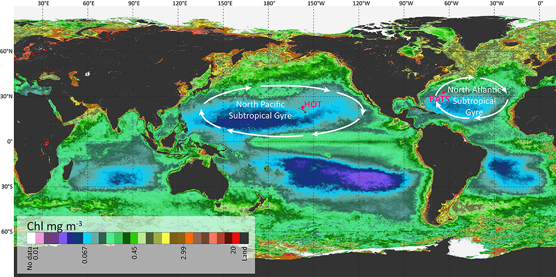
Figure 1. Location of the two stations used in this work: HOT and BATS over a global map representing the annual average of Chl in a color scale.

Both stations are located in waters with a nutrient-limited euphotic zone. On an annual scale, nutrients are higher at surface when vertical mixing is higher, breaking the thermocline, and allowing nutrients to mix into surface waters when a shallower nitracline is observed (Bates et al., 1996; Karl et al., 1996). At HOT, these conditions are found during winter, while at BATS this period occurs in winter and extended to early spring.

The autotrophic community in both regions is dominated by small prokaryotic picoplankton, represented mainly by prochlorophyte and cyanobacteria (e.g., Platt et al., 1983; Siegel et al., 1990; Letelier et al., 1993; Sorensen and Siegel, 2001; Karl and Church, 2017).

In spite of all the environmental similarities between both stations, the primary production cycle from in situ measurement (PP_{in situ}) is different. Nutrients at BATS are rapidly assimilated by phytoplankton and it promotes a short spring phytoplankton bloom between January and March, when PP_{in situ} is maximal (Menzel and Ryther, 1960; Bates et al., 1996; Sorensen and Siegel, 2001). However, this typical seasonal cycle frequently suffers inter-annual changes because of variability in winter mixed layers and surface stratification (Steinberg et al., 2001). Also, other factors such as nutrient injection via mesoscale eddies, or N₂-fixers, had been reported as responsible for seasonally anomalous phytoplankton blooms, that is, in late spring or summer (Steinberg et al., 2001). However, at BATS, such blooms are not strong enough to alter the annual carbon cycle. On the contrary, at HOT the highest PP_{in situ} is generally found during late summer and early fall (Karl and Church, 2017), which pointed to blooms of N₂-fixers as responsible for this alteration in the PP_{in situ} cycle and leading to a maximum in PP_{in situ} in summer.

In situ Datasets

Data at HOT comprised in situ measurements collected concurrently from cruises during the period Mar/1998-Oct/2015. A total of 127 cruises at HOT were used in this work. However, only 47 cruises were found applicable for BATS for the period between Jul/1994 and Mar/2008. For both time series, sampling was conducted at monthly resolution. The protocols applied to data collection and processing are rigorously followed to guarantee consistence in the measurements over time (Sorensen and Siegel, 2001). Additional details of those protocols and collection methods can be found in their respective websites (http://hahana.soest.hawaii.edu/hot/ and http://bats.bios.edu/).

Biogeochemical Measurements

Photosynthetic production of organic matter at different discrete depths (PP_{in situ}, in mg C m⁻³ d⁻¹) was measured by the trace-metal clean ¹⁴C uptake method with incubations performed in situ along one daylight period (dawn-to-dusk) (Fitzwater et al., 1982). In the case of HOT, the depths were 5, 25, 45, 75, 100, and 125 m; while at BATS, the depths were 1, 20, 40, 60, 80, 100, and 120 m. Light- and dark-bottles were incubated in situ following the same procedure and PP_{in situ} was obtained via subtracting dark uptake from light-bottle assimilation. In the case of HOT, dark-bottle incubations were available only in the period Mar/1998-Aug/2000. These values were averaged at depth and subtracted from the light experiments after Oct/2000.

Pigment concentrations (in ng kg⁻¹) from High Performance Liquid Chromatography (HPLC) were measured the same day and at the same depths were PP_{in situ} was estimated.

Optical Measurements

The HOT time-series performed radiometric measurements in water using two different radiometers: Profiler Reflectance Radiometer (PRR600/610, Biospherical Inc.) between March/1998 and August/2009 and Hyperpro free-falling optical profiler, from May/2009. The PRR has 6 spectral bands at 412, 443, 490, 510, 555, and 665 nm, while the Hyperpro is a hyperspectral radiometer, whose sensors measure upwelling radiance and downwelling irradiance (L_u and E_d), respectively, in the visible domain with a spectral resolution of ~10 nm. In the case of BATS, the radiometric profiles were performed using a multispectral radiometer: Multiwavelength Environmental Radiometers (Biospherical Inc., MER-2040, San Diego, CA) up to 1999 and SeaWiFS Profiling Multichannel Radiometer and SeaWiFS Multichannel Surface Radiometer (SPMR/SMSR, Satlantic) after 1999. Those radiometers had 8 and 10 spectral bands, respectively (410, 441, 465, 488, 520, 565, 589, and 665 nm in the case of 8-bands, and additionally at 625 and 683 nm for the 10-bands radiometer). In all the cases, at the same time that the in-water measurements were registered, a radiometer installed above-surface took measurements of solar irradiance (E_S), which were used to correct E_d(z) from cloud effects. The E_d measurements were taken the same day or within one day of difference respect the PP_{in situ} experiment.

Measurements of solar PAR_{in situ} (in μmol photons m⁻² s⁻¹) above surface were registered dawn-to-dusk during the day of PP_{in situ} experiments using a LI-COR LI-1000 integrator/datalogger that registers flux of photons between 400 and 700 nm.

Phytoplankton absorption coefficient (a_{phy,in situ}(λ)) at BATS was estimated during the whole time series following the NASA protocols (NASA, 2003). Seawater was filtered using Whatman GF/F glass fiber filter pads, which were kept frozen in liquid nitrogen until readings (Morrison and Nelson, 2004). Absorption of the filter pad was measured before and after pigment extraction with methanol (Kishino et al., 1985). a_{phy,in situ}(λ) was estimated as a difference between total absorption (before bleaching) and detritus absorption (after bleaching). At HOT, a_{phy,in situ}(λ) was reconstructed by the pigment concentration measured by HPLC (Bidigare et al., 1990; Marra et al., 2000). In this case, it used the unpackaged specific absorption spectra derived from Gaussian approximations and applied the package effect correction available in Wozniak et al. (1999).

Satellite Datasets

Data collected by the MODIS-Aqua sensor between Jul/2002-Dec/2014 were used. The data was downloaded in Level-3 Standard Mapped Image Products, 8-Day composite, in 4-km spatial resolution (https://oceancolor.gsfc.nasa.gov/). Also acquired were the following standard products: Sea Surface Temperature (SST_sat, in °C); Daily Photosynthetically Available Radiation (PAR_day,sat, in mol photons m⁻² d⁻¹) (Frouin et al., 1989); absorption coefficients due to phytoplankton and due to gelbstoff and detrital material at 443 nm [a_phy,_sat(443) and a_dg,_sat(443), respectively, in m⁻¹]; particulate backscattering at 443 nm [b_bp,_sat(443), in m⁻¹]. All the acquired Inherent Optical Properties [a_phy,_sat(443), a_dg,_sat(443) and b_bp,_sat(443)] were estimated through the Generalized Inherent Optical Property (GIOP) model (Werdell et al., 2013). The spectral parameters (S_adg,sat, in nm⁻¹, and S_bb,sat, respectively) required for the derivation of these absorption and backscattering coefficients were processed as in the Quasi-Analytical Algorithm (QAA, Lee et al., 2002). These products were extracted within a 3 × 3 pixel window centered at the geographical coordinates of HOT and BATS stations, average of this window is further estimated for each product to comprise satellite time series between 2002 and 2014.

Data Processing

In situ Data Processing: PP_{in situ}

At HOT, PP_{in situ} was obtained from in situ experiments from Mar/1989 to Oct/2015, while at BATS it was from Jul/1989 to Dec/2016. The integration in the euphotic zone was performed through the trapezoid method (Saba et al., 2010) and included the depths detailed in section Biogeochemical Measurements for both regions.

In situ Data Processing: PAR_day (λ)

The processing to obtain PAR_{day,in situ}(z, λ, expressed in mol photons m⁻² s⁻¹ nm⁻¹) is summarized in the flow-chart in Figure 2.

1) Simulations in Hydrolight (Mobley and Sundman, 2008) were run to estimate E_S(λ) in different conditions that affect solar irradiance at the surface, such as solar zenith angle (0, 30, and 60°), atmospheric visibility (15 and 40 km), cloud percentage (10, 20, 50, 80, and 100%), atmospheric humidity (20, 80, and 100), and atmospheric ozone content (200 and 400). We integrated E_S(λ) (W m⁻²) in the visible domain [E_S(PAR), W m⁻²] and calculated the normalized spectra ${\overline{E}}_S(\lambda )$ as ${\overline{E}}_S(\lambda )=\frac{E_S(\lambda )}{E_S(PAR)}$. ${\overline{E}}_S(\lambda )$ showed a shape well preserved along all the atmospheric conditions tested, with only small differences <8%, toward the blue and red regions. Then we used ${\overline{E}}_S(\lambda )$ to spectrally resolve PAR_{in situ} recorded by LI-COR, by simple multiplication between each LI-COR measurement and ${\overline{E}}_S(\lambda )$ [see ${\overline{E}}_S(\lambda )$ in the Appendix]. In this way, we obtained light variability above surface, and spectrally resolved PP_{in situ} over a day [PAR_{in situ}(0⁺,λ,t)].

2) PAR_{in situ} (0⁺,λ,t) was integrated spectrally and along the day to obtain PAR_{day,in situ} (0⁺) which was used further in section Dynamic temporal parameterization of ϕm and K_ϕ.

3) To estimate PAR_{in situ}(λ) at depth, information about light attenuation is needed. Considering that both stations are located in oligotrophic areas, where water dominates light attenuation for wavelengths >560 nm, and that E_d profiles in wavelengths longer than 560 nm were very noisy, we took the diffuse attenuation coefficient in the range of 561–700 nm [K_{d,in situ}(561–700), m⁻¹] equal to the K_d for pure seawater (K_{d,pure water}). For the wavelengths between 400 and 560 nm, two different processing routines were applied to obtain K_{d,in situ}(λ), according to the type of radiometer used in each cruise (multi- or hyper-spectral).

4) In the case of hyper-spectral data, K_d(400–560) was obtained from Ê_{d,in situ}(z, λ) profiles (Zoffoli et al., 2017), where Ê_{d,in situ}(z, λ) represents measured downwelling spectral irradiance.

5) In the case of multispectral information, the following pertain:

a. The above-water remote sensing reflectance [Rrs_{in situ}(0⁺, λ), in sr⁻¹] was obtained from the profiling measurements following NASA protocol (NASA, 2003) and corrected from Raman effects (Lee et al., 2013).

b. Raman-corrected Rrs_{in situ}(0⁺, λ) was used as input for the QAA v6 algorithm (Lee et al., 2002; Lee, 2014) to obtain a_phy(443), a_dg(443), and b_bp(555). Along with the spectral parameters S_adg and S_bb, these properties were used to generate hyperspectral a_phy, a_dg, and b_bp as in HOPE (Lee et al., 1999).

c. Spectra of total absorption and backscattering coefficients were thus calculated as sum of these components, and then K_d(400–560) was estimated following Lee et al. (2005a), Lee et al. (2013). Being an Apparent Optical Property (AOP), K_d changes with light field. In the above estimation, the change of solar zenith angle (θ_s) was also incorporated, where θ_s was determined based on information of location, day of the year and time of the day.

6) PAR_{in situ}(0⁻,λ,t) together with the K_d(λ,t) allowed the estimation of the irradiance at different depths, every 10 min, for the visible domain [PAR_{in situ}(z,λ, t)] as $PA{R}_{insitu}(z,\lambda ,t)=PA{R}_{insitu}(0^{-},\lambda ,t)·e^{-K_d(\lambda ,t)z}$

7) Finally, PAR_{day,in situ}(z,λ) was estimated by integration of PAR_{in situ}(z,λ,t) between initial and final time of the incubation (sunrise and sunset, respectively).

FIGURE 2

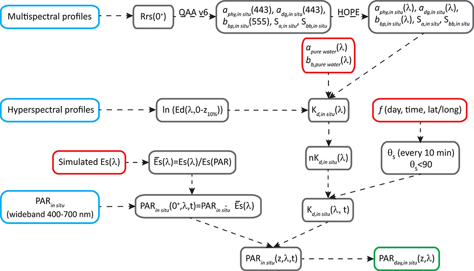
Figure 2. Flow-chart to obtain daily PAR (PAR_{day,in situ}) from in situ data.

In situ Data Processing: ϕ

For each region, cruise, and depth, instantaneous ϕ was estimated from PP_{in situ}(z) and PAR_{day,in situ}(z,λ) following:

$\begin{array}{ll}\varphi (\text{z})=\frac{{\text{PP}}_{\mathit{\text{in situ}}}(\text{z})}{{\displaystyle {\int }_{400}^{700}}{a}_{phy}(\lambda ,\text{z})·{\text{PAR}}_{\text{day},\text{ in situ}}(\text{z},\lambda )\lambda }& (4)\end{array}$

In this approach, a_phy(λ,z) was considered constant over the whole day.

ϕ_m and K_ϕ were further calculated for every cruise/station using the coefficients from a linear fitting of the semi-log graph ln[ϕ(z)] vs. PAR_{day,in situ}(z), where the offset corresponded to ln(ϕ_m). Then, for each cruise, K_ϕ was estimated as value of PAR_{day,in situ} for ϕ equals ϕ_m/2.

Dynamic Temporal Parameterization of ϕ_m and K_ϕ

From the values derived above, monthly ϕ_m and K_ϕ were calculated and smoothed for HOT and BATS. ϕ_m was described as a linear function of the ratio between sea surface temperature (SST) and 20 (SST/20). The value of 20 was chosen as the optimum temperature for carbon fixation and as explained in the discussion. K_ϕ was modeled as a linear function of PAR_{in situ}(0⁺). The results of such parameterization are presented in section Quantum yield of photosynthesis and dynamic parameterizations of ϕm and K_ϕ. After incorporating monthly SST or PAR data obtained from satellite, empirical relationships were developed that well describe the variation of ϕ_m and K_ϕ.

Satellite Data Processing

PP_sat in this work was estimated via two different approaches, with one using the conventional Chl-based scheme (PP_{sat−chl−based}), while the other using the a_phy-based scheme. For both HOT and BATS, the waters were considered homogeneous in the distribution of water constituents. In the case of PP_{sat−chl−based}, the VGPM system (Behrenfeld and Falkowski, 1997b) was used to estimate primary production. In this case, PP_sat is estimated as the integral in the euphotic zone according to Equation 5:

$\begin{array}{l}{\text{PP}}_{\text{sat}-\text{chl}-\text{based}}=0.66125·{\text{P}}_{\text{opt}}^{\text{B}}·\frac{{\text{PAR}}_{\text{sat}}(0^{+})}{({\text{PAR}}_{\text{sat}}(0^{+})+4.1)}\\ ·{\text{z}}_{\text{eu}}·{\text{Chl}}_{\text{sat}}·\text{D}& (5)\end{array}$

where $P_{opt}^B$ is the maximum carbon fixation rate within the water column (mg C mg Chl⁻¹ h^−l), D is day length (in hour) and Chl_sat is the chlorophyll concentration obtained from satellite data. Following Behrenfeld and Falkowski (1997b), ${\text{P}}_{\text{opt}}^{\text{B}}$ was modeled based on SST. We acquired PP_{sat−chl−based} from the Ocean Productivity Home Page (Oregon University) for 8-Day composites in 9 km of spatial resolution between 2002 and 2014. A 1 × 1 pixel window was extracted centered in each station coordinates.

The model proposed by Kiefer and Mitchell (1983) was used to obtain the variation of ϕ caused by light intensities (Equation 3). Here we estimated the integral of PP_sat (Equation 6) for the euphotic zone to be comparable with PP_{sat−chl−based} values. We considered z_eu as 125 m for HOT and 120 m for BATS.

$\begin{array}{l}{\text{PP}}_{\text{sat}-a_{phy}-\text{based}}={\displaystyle {\int }_0^{\text{zeu}}}{\displaystyle {\int }_{400}^{700}}\varphi (\text{z})·a_{phy,\text{sat}}(\lambda )\\ ·{\text{PAR}}_{\text{day},\text{sat}}(\text{z},\lambda )\text{d}\lambda \text{dz}& (6)\end{array}$

As in section in situ data processing: PP_{in situ} for processing multispectral data, a_{phy, sat}(λ) was calculated as a function of a_{phy, sat}(443) following the HOPE model (Lee et al., 1999). Starting from PAR_day,sat, we obtained a PAR_day,sat(λ) by simple multiplication of PAR_sat and the normalized spectrum ${\overline{E}}_S(\lambda )$. K_d,sat for the average daily zenith angle of each 8-Day composite was used to estimate the PAR_day,sat at depth, where $PA{R}_{day,sat}(z,\lambda )=PA{R}_{day,sat}(0^{-},\lambda )·e^{-Kd(\lambda )·z}$. Again, following Lee et al. (2005a, 2013), K_d,sat was calculated from the derived total absorption and backscattering coefficients. The values of ϕ_m and K_ϕ were derived previously in section Dynamic temporal parameterization of ϕ m and Kϕ, and ϕ(z) at depth was calculated as Equation 3.

Method to Evaluate Performance

The satellite and in situ datasets cover different time spans. About 26 years of data comprise the PP_{in situ} data while ~12 years were collected by satellites. Also, the data sampling was performed at different time intervals. In situ experiments lasted one day in ~monthly intervals, while here we used satellite products on an 8-Day composite basis. Not only temporal sampling is different, but also spatial resolution is significantly different. While in situ data came from experiments performed at one location, satellite data came from an integrated area of 9 × 9 km² in the case of PP_{sat−chl−based} and 4 × 4 km² for PP_{sat−aphy−based}. For these reasons, rather than a match-up exercise, we wanted to evaluate whether PP_sat is able to reproduce the overall magnitude and seasonal variations observed in PP_{in situ}. Therefore, differences between monthly median in situ PP (${\widehat{PP}}_{insitu}$) and monthly PP_sat (${\widehat{PP}}_{sat}$) were measured using Unbiased Absolute Percent Difference (UAPD) (Equation 7):

$\begin{array}{ll}\text{UAPD }(\%)=2·\left|({\widehat{\text{PP}}}_{\mathit{\text{in situ}}}-{\widehat{\text{PP}}}_{\text{sat}})\right|/({\widehat{\text{PP}}}_{\mathit{\text{in situ}}}+{\widehat{\text{PP}}}_{\text{sat}})·100& (7)\end{array}$

Results

Quantum Yield of Photosynthesis and Dynamic Parameterizations of ϕ_m and K_ϕ

The derived instantaneous ϕ showed a large range of variability at both stations along the time series and within the water column (Figure 3). Within the period used at BATS (14 years), we had many gaps with incomplete cruise datasets. For this reason, we do not show the timeline for this station. At HOT, minimum and maximum values were ~0.001 and 0.126 mol C mol photons⁻¹, respectively, and corresponded to more than 120-fold of variability. However, more than 95% of the cases were lower than 0.07 mol C mol photons⁻¹, which reduced the variability to 69-fold. A slightly lower range was presented at BATS (~0.002–0.121 mol C mol photons⁻¹), which corresponded to 50-fold of variability. Restricting instantaneous ϕ to 95% of the occurrences, it varies in a range of ~0.002–0.1 mol C mol photons⁻¹, reducing its variability to 45-fold.

FIGURE 3

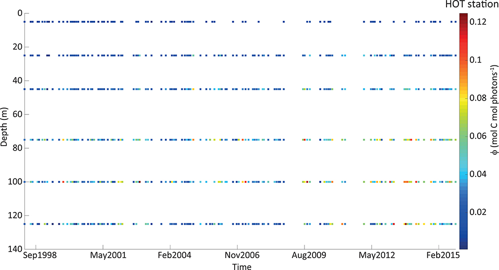
Figure 3. Quantum yield of photosynthesis (ϕ, in mol C mol photons ⁻¹) estimated from in situ measurements at HOT station, represented in a colorimetric scale (exhibited on the right). The vertical axis shows the depth in meters (from 0 on the top to deeper values on the bottom). The horizontal axis represents time and every point in the graph corresponds to a monthly cruise.

As expected, the highest variability in the ϕ was observed vertically, with the lowest values at the surface and the highest at depth (Figure 4A). This pattern was opposite to the vertical distribution of PP_{in situ} (Figure 4B). While PP_{in situ} is ruled mainly by light availability, the highest efficiencies are found at deeper depths. The maximum values of the instantaneous ϕ in both stations almost attained the maximum theoretical value and they were observed at great depths with very low light levels. On some cruises, the ϕ obtained at the greatest depths surpassed the theoretical maximum of 0.125 mol C mol photons⁻¹. At those depths, both PP_{in situ} and light levels are very low, thus potentially creating very high uncertainties in the estimated ϕ due to difficulties in obtaining accurate PP_{in situ} and light intensity at such low values. Therefore, any ϕ values higher than 0.125 mol C mol photons⁻¹ were omitted and we have ignored depths >80 m to avoid estimations subjected to high uncertainties.

FIGURE 4

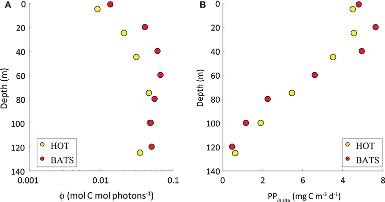
Figure 4. (A) Annual average of the quantum yield of photosynthesis (ϕ, in mol C mol photons ⁻¹) in a vertical scale. The abscissa axis represents ϕ exhibited in log-scale (mol C mol photons⁻¹) and the ordinate axis shows depth (in m). (B) PP_{in situ} (mg C m⁻³ d⁻¹) along the water column. In both graphs, yellow dots represent HOT and red dots, BATS.

We observed a consistent seasonal variability in the instantaneous ϕ in both stations during the whole time series. Also, in situ ϕ_m and K_ϕ showed temporal variabilities. At HOT, higher ϕ_m values were found during winter (Jan–Feb), but the range of variability is quite narrow (monthly median is 0.038–0.045 mol C mol photons⁻¹ except January) (Figure 5A). Instead, at BATS, the highest ϕ_m was observed for a longer season, from Fall to Winter (Oct–Mar), with a higher seasonal variability (monthly median 0.050–0.096 mol C mol photons⁻¹) (Figure 5B). According to previous works (e.g., Bates et al., 1996), the higher photosynthetic efficiency found in Fall-Winter can be related to the position of the thermocline and, therefore, to injection of nutrients into the euphotic zone. In both regions, between Summer and Spring the photosynthetic efficiency remained low.

FIGURE 5

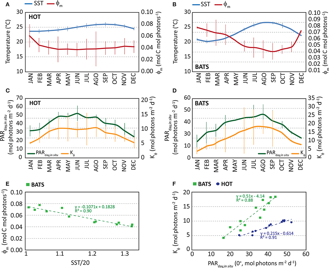
Figure 5. Monthly median of in situ maximum quantum yield of photosynthesis (ϕ_m, in mol C mol photons ⁻¹) in red and in situ monthly median of sea surface temperature (SST, in °C) in blue: (A) at HOT and (B) at BATS. Error bars represent standard deviation. Monthly median of in situ K_ϕ (in mol photons m⁻² d⁻¹) in yellow and in situ monthly median of PAR_{day,in situ} (in mol photons m⁻² d⁻¹) in green: (C) at HOT and (D) at BATS. Error bars represent standard deviation. (E) In situ monthly median ϕ_m as a function of monthly SST at BATS and (F) in situ monthly median K_ϕ as a function of PAR_{day,in situ} (0⁺). In graph and (F) results of both stations are displayed together, where HOT is represented by blue circles and BATS as green squares.

On the other hand, K_ϕ is found following the temporal variability of PAR_day(0⁺), with the highest values in Summer and the lowest in Winter (Figures 5C,D). Comparing both stations, a higher annual median value was observed in ϕ_m at BATS, suggesting a higher photosynthetic efficiency during the whole year. K_ϕ was higher at BATS as well. Also at BATS, the monthly variability in the parameters was found higher than HOT, even though both stations were located in oligotrophic waters of the North Subtropical Gyres. Estimated median annual values of ϕ_m were 0.0395 and 0.063 mol C mol photons⁻¹ at HOT and BATS, respectively; while K_ϕ values were 8.0 and 10.8 mol photons m⁻² d⁻¹, respectively. The seasonal patterns found in both parameters and stations led us to incorporate temporal variation in the model through a dynamical modeling of ϕ_m and K_ϕ, (Figures 5E,F) as presented below:

$\begin{array}{l}{\varphi }_{\text{m}}=-0.0451·(\frac{\text{SST}}{20})+0.098,\\ \text{and }{\varphi }_{\text{m}}\le 0.125\text{ mol C }{\text{mol photons}}^{-1}& (8)\end{array}$

$\begin{array}{ll}{\text{K}}_{\varphi }=0.215·{\text{ PAR}}_{\text{day},\mathit{\text{in situ}}}(0^{+})-0.614& (9)\end{array}$

$\begin{array}{l}{\varphi }_{\text{m}}=-0.1071·(\frac{\text{SST}}{20})+0.1828,\\ \text{and }{\varphi }_{\text{m}}\le 0.125\text{ mol C }{\text{mol photons}}^{-1}& (10)\end{array}$

$\begin{array}{ll}{\text{K}}_{\varphi }=0.51·{\text{ PAR}}_{\text{day},\mathit{\text{in situ}}}(0^{+})-4.14& (11)\end{array}$

Here, Equations 8, 9 correspond to parameterizations for ϕ_m and K_ϕ at HOT (regression analysis for ϕ_m vs. (SST/20): R² = 0.17, p = 0.183, for K_ϕ vs. PAR: R² = 0.91, p = 1.7 10⁻⁶, at 95% confidence level); while Equations 10-11 are used at BATS (regression analysis for ϕ_m vs. (SST/20): R² = 0.90, p = 2.89 10⁻⁶, for K_ϕ vs. PAR: R² = 0.88, p = 8.22 10⁻⁶, at 95% confidence level). The p-values suggest significance in models, except for the quadratic relation between ϕ_m and (SST/20) at HOT. The narrow variability not only in monthly ϕ_m but also in SST, explains its lack of significance in the parameterization for HOT. For this reason, we did not incorporate this parameterization into the instantaneous ϕ modeling but decided to keep it constant and equal to the median annual value (0.0395 mol C mol photons⁻¹).

Median values of ϕ_m and K_ϕ resulted from the above modeling were similar to those found in situ, even when they were derived from different inputs and slightly different periods of time (Figure 6). Median ϕ_m was 0.060 mol C mol photons⁻¹ at BATS. K_ϕ resulted in 9.5 mol photons m⁻² d⁻¹ at HOT and higher at BATS (15.7 mol photons m⁻² d⁻¹). At BATS, the modeled ϕ_m from SST_sat showed higher values in Fall-Winter and the lowest in Summer, following the in situ pattern. Sorensen and Siegel (2001) found a similar relationship between ϕ_m and SST at BATS. Even though the correlation was weak, it seems that SST is a good predictor for ϕ_m over the year, thus allowing an effective temporal modeling of ϕ_m. The temporal pattern of K_ϕ modeled with PAR_day,sat, was the same as that observed in situ at the two stations.

FIGURE 6

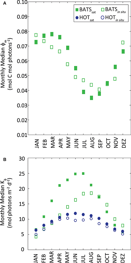
Figure 6. (A) Monthly median ϕ_m as a function of monthly SST and (B) monthly median K_ϕ as a function of PAR. Station HOT is displayed as blue circles and BATS as green squares. Filled markers refer to parameters obtained from satellite measurements; empty markers correspond to the same parameters from in situ data.

PP by Satellite

Comparing PP_{sat−chl−based} with PP_{in situ}, the performance by the default VGPM for the two stations is different (Figure 7). At HOT, the PP_{sat−chl−based} presented a strong underestimation with average difference of 62.8%, and a seasonal pattern opposite to in situ measurements (R² = 0.27). At BATS, the performance was better than that at HOT, with mean AUPD of 37.8%. At BATS the seasonal cycle was similar to that of in situ measurements (R² = 0.34), but with a delay of 3–4 months in the minimum and a shorter length on the maximum.

FIGURE 7

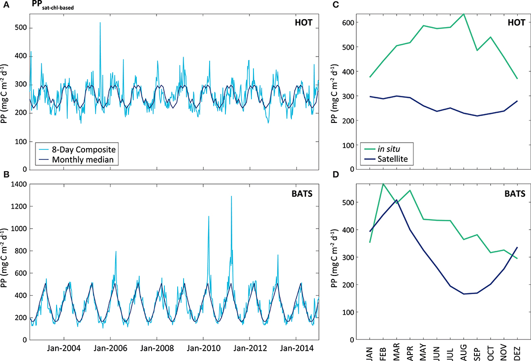
Figure 7. PP_sat (expressed in mg C m⁻² d⁻¹) obtained through the VGPM model, Chl-based. The light blue line represents the results obtained for the 8-Day composite, while the dark blue represents the monthly median calculated for these data, at HOT (A) and BATS (B). The graphs on the right shows a comparison between satellite and in situ PP estimates (monthly median of the PP_{sat−chl−based} in the blue line, and monthly median of the PP_{in situ} in the green line), for HOT (C) and BATS (D).

On the contrary, the PP_{sat−aphy−based} model with the dynamic parameterization of ϕ considerably reduces the differences between satellite estimates and in situ measurements at HOT. In this area, UAPD reduced to only 8.3%. At BATS, UAPD remains about the same (36.4%). However, results are improved when observing the seasonal pattern. PP_{sat−aphy−based} is able to well reproduce the PP seasonal cycle in both areas (R² = 0.76 at HOT; R² = 0.71 at BATS, Figure 8). The summer maximum of PP_{sat−aphy−based} matches the in situ findings. The overestimation of the PP peak at BATS still needs to be inspected. Interestingly, the highest instantaneous ϕ, which is a function of both ϕ_m and K_ϕ, does not correspond to the maximum PP at HOT (Figure 9). Even when the ϕ is highest in winter, the PP peak was predicted to be during summer. The quantum yield of photosynthesis is not exclusively nutrient-driven nor light-driven but a combination of both factors (Sorensen and Siegel, 2001), which explains its large temporal variability. However, it is important to keep in mind that the instantaneous ϕ is not the only parameter responsible for PP, but also the phytoplankton absorption (which is related to its abundance) and light availability. Note that even though the temporal pattern of PP_{in situ} is different, both PAR and a_phy showed a similar seasonal variation comparing both stations (Figure 10). We also run the PP_{sat−aphy−based} model using annual median values of ϕ_m and K_ϕ instead of the dynamic parameterization, as a way to evaluate the impact of the temporal variability in those parameters on predicting PP. In this case, at HOT the temporal response of PP generally followed the in situ values with lower correlation (R² = 0.70) (Figure 8C, red curve), and slightly lower performance in terms of magnitude, with AUPD of 9.1%. At BATS, however, using fixed parameters PP showed a similar AUPD (35.2%) but a worse response in terms of the seasonal pattern (R² = 0.53) with a secondary peak of PP during summer not observed in situ (Figure 8D, red curve). These findings support then the need of regional in situ measurements and incorporating temporal dependence on photosynthetic parameters according to the study area. It is exactly the efficiency in the conversion from light into fixed C (this is the ϕ) that conforms satellite measurements into the real environmental observations, and thus fixed values for ϕ_m and K_ϕ would limit the capability to produce consistent observations for the global oceans.

FIGURE 8

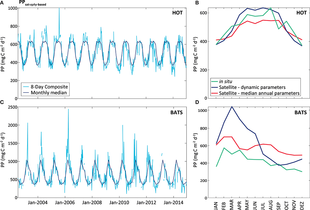
Figure 8. PP_sat (expressed in mg C m⁻² d⁻¹) obtained through the a_phy model using temporal dynamic parameterization. The light blue line represents the results obtained for the 8-Day composite, while the dark blue represents the monthly median calculated for these data, at HOT (A) and BATS (B). The graphs on the right shows a comparison between satellite and in situ PP estimates (monthly median of the PP_{sat−aphy−based} using our dynamic parameterization in the blue line, monthly median of the PP_{sat−aphy−based} using both parameters as constant in the red line, and monthly median of the PP_{in situ} in the green line), for HOT (C) and BATS (D).

FIGURE 9

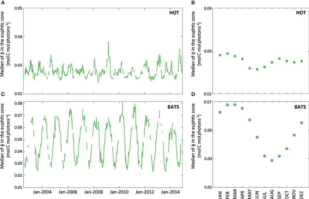
Figure 9. Average of instantaneous ϕ (expressed in mol C mol photons⁻¹) within the euphotic zone obtained through MODIS-Aqua data for the whole data series (2002–2014). The green line represents the median of instantaneous ϕ for the euphotic zone (A) at HOT and (B) BATS. Aside, graphs (C) and (D) show the monthly median of ϕ for each of the stations obtained from satellite.

FIGURE 10

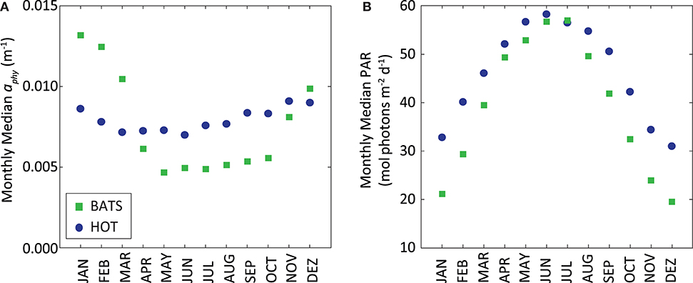
Figure 10. (A) Monthly median of MODIS-Aqua a_phy (m⁻¹) and (B) monthly median of MODIS-Aqua PAR (mol photons m⁻² d⁻¹) at surface. In both graphs stations HOT (blue circles) and BATS (green squares) are displayed together.

Discussion

In this work, we estimated ϕ_m and K_ϕ from in situ measurements. According to their temporal behavior, we modeled ϕ_m and K_ϕ based on in situ measurements as function of environmental parameters. At HOT, in situ median value of ϕ_m was equal to 0.04 mol C mol photons⁻¹. While at BATS, annual median values of ϕ_m were found between ~0.06 mol C mol photons⁻¹ from both methods. K_ϕ varied between 8 and 16 mol photons m⁻² d⁻¹ for both, stations and methods. These magnitudes are in good agreement with such values provided in other works. Kiefer and Mitchell (1983) found ϕ_m as 0.06 mol C mol photons⁻¹ and K_ϕ as 10 mol photons m⁻² d⁻¹ from laboratory analysis using monocultures of a diatom species and varying nutrient and light levels. Morel (1978) estimated ϕ_m in the Sargasso Sea from in situ measurements and found an average of 0.03 mol C mol photons⁻¹. In a work developed at BATS from the same dataset (Sorensen and Siegel, 2001), it was found an average ϕ_m ~0.035 mol C mol photons⁻¹. This value is slightly lower than the values presented in this work, but in this case the same seasonal pattern with the lowest ϕ_m in summer. Also in the referred work, K_ϕ was 16 mol photons m⁻² d⁻¹, a bit higher than that obtained here. These differences can be caused by differences in the time period used in both works and the inputs [a_phy and E_d(z)] used to derive those parameters. Morel (1978) considered only two cruises (in May/1970 and March-April/1974 totalizing 32 stations) and Sorensen and Siegel (2001) used only 5 years of data. We included 14 years of measurements.

The dynamic parameterization we adopted was SST_sat for the estimation of ϕ_m at BATS and PAR_day(0⁺) for K_ϕ in the two regions. It is known that phytoplankton have an optimum temperature for growth and photosynthesis (Li, 1980). Lower temperatures mean physiological restrictions in the metabolism of the Calvin Cycle (Falkowski, 1980). Above such an optimum, there are also metabolic restrictions linked to protein inactivation and denaturation (Ratkowsky et al., 1983). Figure 11 illustrates the ${\text{P}}_{\text{opt}}^{\text{B}}$ parameter, used by the VGPM. This parameter shows the maximum C fixation rate within a water column, and is obtained from a polynomic function that depends only on SST. It expresses the metabolic functioning of phytoplankton and we use it here to show the relation between temperature and physiology. Note that SST_sat in this region in the period 2002–2014 ranges within narrow intervals:18–28.8°C, and the optimum temperature seems to be ~20°C and not at the highest values observed. Besides physiology, temperature and nutrient inputs could also be related in the euphotic zone. Even though no nutrients were analyzed in this work, periods with the highest ϕ_m are perceived to follow the nutrient injection to surface, facilitated by the breakdown of the thermocline and vertical recirculation in the water column (Figures 5B,C), which implies lower temperatures. There appears to be a reduction in metabolic rates under 20°C. However, during winter conditions, nutrient concentration was expected to be the highest, stimulating phytoplankton production and overriding any limitation caused by temperatures being under its optimum. This relation between ϕ_m, temperature, and nutrients explains the inverse relation between ϕ_m and SST_sat, supporting the idea of using this environmental parameter to model ϕ_m. The exploration of this relationship should be evaluated carefully at higher latitudes, where temperatures in winter can drop considerably thus the impact to ϕ_m separated from that by nutrient would be complex. Also, coastal environments can behave differently and SST_sat would not necessarily be a good proxy of the ϕ_m, since nutrient input also has a terrestrial contribution in addition to vertical stratification and the position of the thermocline.

FIGURE 11

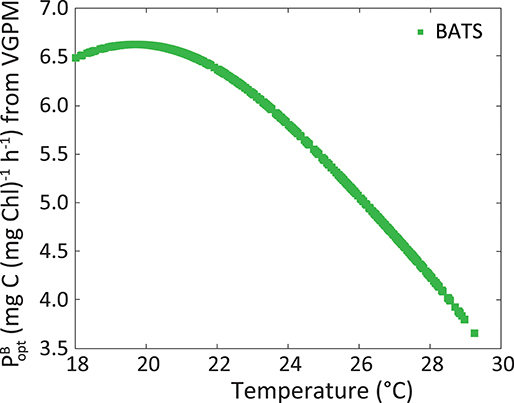
Figure 11. Maximum C fixation rate within a water column [${\text{P}}_{\text{opt}}^{\text{B}}$, in mg C (mg Chl)⁻¹ h⁻¹] following VGPM, as a function of SST_sat at BATS.

It was shown here temporal variability of ϕ_m and K_ϕ estimated from in situ experiments of PP_{in situ} and measurements of E_d and PAR at surface. Such estimation was only possible thanks to the effort of many people engaged to maintain long time-series measurements, with careful collection methods at HOT and BATS. These activities should be encouraged worldwide as we see that in situ observations are critical for calibration and validation activities into remote sensing science to allow it to provide reliable products. It appears that there is a better performance at HOT than at BATS, likely because we have a much bigger data pool at HOT than at BATS for the derivation of ϕ_m and K_ϕ. It thus allowed a better calibration of the model in the Pacific Ocean, improving PP_{sat−aphy−based} performance. Also at BATS, the number of samples during some months (Jan, May, Nov, and Dec) was a bit lower than other months considering the coefficient of variation. Sorensen and Siegel (2001) showed a difference up to 40% along 4 consecutive days at BATS, exemplifying how highly noisy PP_{in situ} can be. This suggests that, even with a great effort in keeping a long time-series of 26 years, in situ sampling could not be sufficient during some periods to capture the real variability that could explain differences between PP_{in situ} and PP_{sat−aphy−based}.

Within vegetal cells, only chlorophyll-a contributes to photosynthesis. Based on this premise, the PP_{sat−chl−based} methods propose that PP can be directly estimated from Chl. However, there are some caveats in estimating PP with this strategy. First, even when Chl has been widely considered an indicator of phytoplankton biomass it is also known that Chl is a weak indicator of it (Behrenfeld et al., 2005, 2016; Bellacicco et al., 2016). It has been demonstrated that pigment concentration is dependent on the phytoplankton group, cell size, light availability, nutritional state of the cells, meaning that the same Chl value can be found in waters with different abundance of phytoplankton. Second, there are other accessory pigments in phytoplankton cells that also capture photons, which can be transmitted to chlorophyll-a and used in photosynthesis (if they are photosynthetic pigments, as for example, chlorophyll-b and -c) or this energy is lost as heat (when the implicated pigments are photoprotective, as for example diadinoxanthin and diatoxanthin) (Ostrowska et al., 2012). On the other hand, not all chlorophyll-a is active for photosynthesis. It is well known that it can exist as a “package” inside the cell, which means the capacity to absorb photons can be different even for the same Chl value. But these are not the only factors to take into account when evaluating the result of PP_{sat−chl−based} models. Satellite sensors actually measures radiometric magnitude (i.e., radiance). The direct parameters we can derivate from those satellite measurements are, then, optical parameters (absorption, backscattering) rather than biological information such as Chl, which constitutes a secondary measurement. This suggests that PP_{sat−aphy−based}, that uses a phytoplankton absorption coefficient as input, reduces uncertainties in model inputs. In this context, ϕ is a key parameter that introduces biological information into the model that converts optical (absorbed light) into biological information (PP).

It is exactly to those optical and photophysiological parameters to whom researchers have attributed the responsibility for the low performance found in some PP_sat models that have been commonly applied (Platt et al., 1991; Morel et al., 1996; Bouman et al., 2000). Kovač et al. (2017) also point to the relation between the rate of carbon assimilation by phytoplankton and light as the core parameters that convert stocks of C (the immediate image taken by satellite) into a rate (PP). We demonstrated here that actually questionable photophysiological parameters are responsible for high uncertainties observed frequently in PP_sat results. In fact, the mathematical formulation of the PP_{sat−aphy−based} and the optical inputs appear to be adequate. The part of the model that is still a challenge is in the linkage between optics and biology, that is, the quantum yield of photosynthesis. More efforts into the estimation of global ocean PP via satellite remote sensing should be allocated to in situ sampling to provide data to model this parameter. We showed that appropriate, spectrally resolved, inputs [a_phy(λ) and E_d(z, λ)] combined with regionalized biological parameters reduce such uncertainties in producing reliable PP estimates over the years. This work shows also an example of how important regional studies are, and that the same biome in two different places, oligotrophic gyres in this case, can present different temporal behaviors in photosynthetic restrictions. We suggest that the formula to provide good estimates of oceanic primary production in the global ocean seems to be combining satellite observations with regionalized dynamical parameterization based on in situ measurements and using biogeochemical provinces as a frame for such regionalization.

Conclusions

Temporal and regional variability were observed in photophysiological parameters ϕ_m and K_ϕ estimated from decades of in situ measurements. At HOT, into the North Pacific Subtropical Gyre, the median annual values for ϕ_m and K_ϕ were 0.040 mol C mol photons⁻¹ and 8.0 mol photons m⁻² d⁻¹, respectively. Slightly higher values were found for both at BATS, located in the North Atlantic Subtropical Gyre, where ϕ_m was found equal to 0.063 mol C mol photons⁻¹ and K_ϕ of 10.8 mol photons m⁻² d⁻¹. In both regions, highest values of ϕ_m occurred in the Fall-Winter period, coinciding with the highest nutrient concentration. The peak of K_ϕ, on the contrary, was found in Summer, following seasonality in PAR. SST and PAR_day(0⁺) were chosen as proxies to estimate temporal variability of ϕ_m and K_ϕ, respectively. However, at HOT, seasonal variability seems negligible for ϕ_m and we kept it as a constant in this region equal to the annual median value derived from in situ measurements. Our dynamic parameterization was tested using satellite information and further applied to the PP_{sat−aphy−based} model. The values found from such dynamic parameterization were within the same range as those from in situ measurements: 0.060 mol C mol photons⁻¹ for ϕ_m at BATS, and 9.5 and 15.7 mol photons m⁻² d⁻¹ for K_ϕ, corresponding to HOT and BATS, respectively. Comparing with in situ measurements, the PP_{sat−aphy−based} showed the same temporal variability, with differences of only 8.3% at HOT and 36.4% at BATS when our dynamic parameterization was used. These differences were lower than the ones found using a default PP_{sat−chl−based} model at HOT which resulted in 62.8% difference, and similar at BATS, with AUPD of 37.8%. However, in terms of the seasonal pattern the PP_{sat−chl−based} model performed worse in both areas (R² = 0.27 and 0.34 at HOT and BATS, respectively) and an opposite seasonal pattern at HOT. Our results strongly suggest that an effort to regionally parameterize ϕ_m and K_ϕ from in situ data can significantly improve PP_sat, to provide then, solid estimates of primary production of the global oceans.

Author Contributions

MZ conceptualization, data processing and analysis, investigation, methodology, writing–original draft. ZL conceptualization, data analysis, investigation, methodology, writing–original draft, funding acquisition, project administration, resources. JM conceptualization, data analysis, writing–original draft.

Funding

Funding for this study was provided by National Aeronautic and Space Administration (NNX14AM15G, NNX14AQ47A).

Conflict of Interest Statement

The authors declare that the research was conducted in the absence of any commercial or financial relationships that could be construed as a potential conflict of interest.

Acknowledgments

The measurements and data collected at HOT and BATS are greatly appreciated. We thank NASA OBPG for providing products from ocean color satellite measurements, and two reviewers to improve this manuscript.

References

Babin, M., Morel, A., Claustre, H., Bricaud, A., Kolbert, Z., and Falkowski, P. G. (1996). Nitrogen- and irradiancedependent variations of the maximum quantum yield of carbon fixation in eutrophic, mesotrophic and oligotrophic marine systems. Deep-Sea Res. Part I. 43, 1241–1272. doi: 10.1016/0967-0637(96)00058-1

CrossRef Full Text | Google Scholar

Bates, N. R., Michaels, A. F., and Knap, A. H. (1996). Seasonal and interannual variability of oceanic carbon dioxide species at the U.S. JGOFS bermuda atlantic time-series study (BATS) site. Deep-Sea Res. Part II. 43, 347–383. doi: 10.1016/0967-0645(95)00093-3

CrossRef Full Text | Google Scholar

Behrenfeld, M. J., Boss, E. S., Siegel, D. A., and Shea, D. M. (2005). Carbon-based ocean productivity and phytoplankton physiology from space. Global Biogeochem. Cycles 19:GB1006. doi: 10.1029/2004GB002299

CrossRef Full Text | Google Scholar

Behrenfeld, M. J., and Falkowski, P. G. (1997a). A consume's guide to phytoplankton primary productivity models. Limnol. Oceanogr. 42, 1479–1491.

Google Scholar

Behrenfeld, M. J., and Falkowski, P. G. (1997b). Photosynthetic rates derived from satellite-based chlorophyll concentration. Limnol. Oceanogr. 42, 1–20. doi: 10.4319/lo.1997.42.1.0001

CrossRef Full Text | Google Scholar

Behrenfeld, M. J., O'Malley, R. T., Boss, E. S., Westberry, T. K., Graff, J. R., Halsey, K. H., et al. (2016). Revaluating ocean warming impacts on global phytoplankton. Nat. Clim. Chang. 6, 323–330. doi: 10.1038/nclimate2838

CrossRef Full Text | Google Scholar

Behrenfeld, M. J., Randerson, J. T., McClain, C. R., Feldman, G. C., Los, S. O., Tucker, C. J., et al. (2001). Biospheric primary production during an ENSO transition. Science 291, 2594–2597. doi: 10.1126/science.1055071

PubMed Abstract | CrossRef Full Text | Google Scholar

Bellacicco, M., Volpe, G., Colella, S., Pitarch, J., and Santoleri, R. (2016). Influence of photoacclimation on the phytoplankton seasonal cycle in the mediterranean sea as seen by satellite. Remote Sens. Environ. 184, 595–604. doi: 10.1016/j.rse.2016.08.004

CrossRef Full Text | Google Scholar

Bidigare, R., Michael, E. O., Morrow, J. H., and Kiefer, D. A. (1990). In vivo absorption properties of algal pigments. Proc. SPIE–Int. Soc. Opt. Eng. 1302, 290–302.

Google Scholar

Bouman, H. A., Platt, T., Sathyendranath, S., Irwin, B. D., Wernand, M. R., and Kraay, G. W. (2000). Bio-optical properties of the Subtropical North Atlantic. II. relevance to models of primary production. Mar. Ecol. Prog. Ser. 200, 19–34. doi: 10.3354/meps200019

CrossRef Full Text | Google Scholar

Campbell, J., Antoine, D., Armstrong, R., Arrigo, K., Balch, W., Barber, R., et al. (2002). Comparison of algorithms for estimating ocean primary production from surface chlorophyll, temperature, and irradiance. Global Biogeochem. Cy. 16:1035. doi: 10.1029/2001GB001444

CrossRef Full Text | Google Scholar

Carder, K. L., Lee, Z., Marra, J., Steward, R. G., and Perry, M. J. (1995). Calculated quantum yield of photosynthesis of phytoplankton in the marine light-mixed layers (59-Degrees-N, 21-Degrees-W). J. Geophys. Res. Oceans 100, 6655–6663. doi: 10.1029/94JC02793

CrossRef Full Text | Google Scholar

Carr, M. E., Friedrichs, M. A. M., Schmeltz, M., Noguchi Aita, M., Antoine, D., Arrigo, K. R., et al. (2006). A comparison of global estimates of marine primary production from ocean color. Deep-Sea Res. II. 53, 741–777. doi: 10.1016/j.dsr2.2006.01.028

CrossRef Full Text | Google Scholar

Falkowski, P. G. (1980). “Light-shade adaptation in marine phytoplankton”, in Primary Productivity in the Sea, ed P. Falkowski (New York, NY: Plenum Press), 99–119.

PubMed Abstract | Google Scholar

Field, C. B., Behrenfeld, M. J., Randerson, J. T., and Falwoski, P. G. (1998). Primary production of the biosphere: integrating terrestrial and oceanic components. Science 281, 237–240. doi: 10.1126/science.281.5374.237

PubMed Abstract | CrossRef Full Text | Google Scholar

Finenko, Z. Z., Churilova, T. Y., Sosik, H. M., and Basturk, O. (2002). Variability of photosynthetic parameters of the surface phytoplankton in the Black Sea. Okeanologiya 42, 53–67.

Google Scholar

Fitzwater, S. E., Knauer, G. A., and Martin, J. H. (1982). Metal contamination and its effects on primary production measurements. Limnol. Oceanogr. 27, 544–551. doi: 10.4319/lo.1982.27.3.0544

CrossRef Full Text | Google Scholar

Frouin, R., Lingner, D. W., Gautier, C., Baker, K. S., and Smith, R. C. (1989). A simple analytical formula to compute clear sky total and photosynthetically available solar irradiance at the ocean surface. J. Geophys. Res. 94, 9731–9742. doi: 10.1029/JC094iC07p09731

CrossRef Full Text | Google Scholar

Hirawake, T., Takao, S., Horimoto, N., Ishimaru, T., Yamaguchi, Y., and Fukuchi, M. (2011). A phytoplankton absorption-based primary productivity model for remote sensing in the Southern Ocean. Polar Biol. 34, 291–302. doi: 10.1007/s00300-010-0949-y

CrossRef Full Text | Google Scholar

Iluz, D., and Dubinsky, Z. (2013). “Quantum yields in aquatic photosynthesis”, in Photosynthesis, ed Z. Dubinsky (IntechOpen), 135–158. doi: 10.5772/56539

CrossRef Full Text | Google Scholar

Karl, D. M., Christian, J. R., Dore, J. E., Hebel, D. V., Letelier, R. M., Tupas, L. M., et al. (1996). Seasonal and interannual variability in primary production and particle flux at station ALOHA. Deep-Sea Res. Part II. 43, 539–568. doi: 10.1016/0967-0645(96)00002-1

CrossRef Full Text | Google Scholar

Karl, D. M., and Church, M. J. (2017). Ecosystem structure and dynamics in the north pacific subtropical gyre: new views of an old ocean. Ecosystems 20, 433–457. doi: 10.1007/s10021-017-0117-0

CrossRef Full Text | Google Scholar

Kiefer, D., and Mitchell, B. G. (1983). A simple, steady state description of phytoplankton growth based on absorption cross section and quantum efficiency. Limnol. Oceanogr. 28, 770–776. doi: 10.4319/lo.1983.28.4.0770

CrossRef Full Text | Google Scholar

Kishino, M., Takahashi, M., Okami, N., and Ichimura, S. (1985). Estimation of the spectral absorption coefficients of phytoplankton in the sea. Bull. Mar. Sci. 37, 634–642.

Google Scholar

Kolber, Z. S., Prasil, O., and Falkowski, P. G. (1998). Measurements of variable chlorophyll fluorescence using fast repetition rate techniques: defining methodology and experimental protocols. Biochim. Biophys. Acta 1367, 88–106. doi: 10.1016/S0005-2728(98)00135-2

CrossRef Full Text | Google Scholar

Kovač, Ž., Platt, T., Sathyendranath, S., and Antunović, S. (2017). Models for estimating photosynthesis parameters from in situ production profiles. Prog. Oceanogr. 159, 255–266. doi: 10.1016/j.pocean.2017.10.013

CrossRef Full Text | Google Scholar

Lee, Z. (2014). Update of the Quasi-Analytical Algorithm (QAA_v6). Dartmouth: International Ocean Colour Coordinating Group. Available online at: http://www.ioccg.org/groups/Software_OCA/QAA_v6_2014209.pdf

Google Scholar

Lee, Z., Carder, K. L., and Arnone, R. A. (2002). Deriving inherent optical properties from water color: a multiband quasi-analytical algorithm for optically deep waters. Appl. Opt. 41, 5755–5772. doi: 10.1364/AO.41.005755

PubMed Abstract | CrossRef Full Text | Google Scholar

Lee, Z., Carder, K. L., Mobley, C. D., Steward, R. G., and Patch, J. S. (1999). Hyperspectral remote sensing for shallow waters. 2. deriving bottom depths and water properties by optimization. Appl. Opt. 38, 3831–3843.

PubMed Abstract | Google Scholar

Lee, Z., Du, K., and Arnone, R. (2005a). A model for the diffuse attenuation coefficient of downwelling irradiance. J. Geophys. Res. Oceans. 110, 1–10. doi: 10.1029/2004JC002275

CrossRef Full Text | Google Scholar

Lee, Z., Du, K., Arnone, R., Liew, S. C., and Penta, B. (2005b). Penetration of solar radiation in the upper ocean – a numerical model for oceanic and coastal waters. J. Geophys. Res. 110:C09019. doi: 10.1029/2004JC002780

CrossRef Full Text | Google Scholar

Lee, Z., Hu, C., Shang, S., Du, K., Lewis, M., Arnone, R., et al. (2013). Penetration of UV-visible solar radiation in the global oceans: insights from ocean color remote sensing. J. Geophys. Res. Oceans. 118, 4241–4255. doi: 10.1002/jgrc.20308

CrossRef Full Text | Google Scholar

Lee, Z., Lance, V. P., Shang, S., Vaillancourt, R., Freeman, S., Lubac, B., et al. (2011). An assessment of optical properties and primary production derived from remote sensing in the southern ocean (SO GasEx). J. Geophys. Res. 116, 1–15. doi: 10.1029/2010JC006747

CrossRef Full Text | Google Scholar

Lee, Z., Marra, J., Perry, M. J., and Kahru, M. (2015). Estimating oceanic primary productivity from ocean color remote sensing: a strategic assessment. J. Mar. Syst. 149, 50–59. doi: 10.1016/j.jmarsys.2014.11.015

CrossRef Full Text | Google Scholar

Lee, Z. P., Carder, K. L., Marra, J., Steward, R. G., and Perry, M. J. (1996). Estimating primary production at depth from remote sensing. Appl. Opt. 35, 463–474. doi: 10.1364/AO.35.000463

PubMed Abstract | CrossRef Full Text | Google Scholar

Letelier, R. M., Bidigare, R. R., Hebel, D. V., Ondrusek, M., Winn, C. D., and Karl, D. M. (1993). Temporal variability of phytoplankton community structure based on pigment analysis. Limnol. Oceanogr. 38, 1420–1437. doi: 10.4319/lo.1993.38.7.1420

CrossRef Full Text | Google Scholar

Li, W. K. W. (1980). “Temperature adaptation in phytoplankton: cellular and photosynthetic characteristics”, in Primary Productivity in the Sea, ed P. Falkowski (New York, NY: Plenum Press), 259–279.

Google Scholar

Longhurst, A., Sathyendranath, S., Platt, T., and Caverhill, C. (1995). An estimate of global primary production in the ocean from satellite radiometer data. J. Plankton Res. 17, 1245–1271. doi: 10.1093/plankt/17.6.1245

CrossRef Full Text | Google Scholar

Ma, S., Tao, Z., Yang, X., Ma, W., Yu, Y., Zhou, X., et al. (2014). Estimation of marine primary productivity from satellite-derived phytoplankton absorption data. J-STARS 7, 3084–3092. doi: 10.1109/JSTARS.2014.2298863

CrossRef Full Text | Google Scholar

Marra, J., Chamberlain, W. S., and Knudson, C. (1993). Proportionality between in situ carbon assimilation bio-optical measures of primary production in the gulf of maine in summer. Limnol. Oceanogr. 38, 232–238. doi: 10.4319/lo.1993.38.1.0232

CrossRef Full Text | Google Scholar

Marra, J., Trees, C. C., Bidigare, R. R., and Barber, R. T. (2000). Pigment absorption and quantum yields in the Arabian Sea. Deep-Sea Res. Part I. 47, 1279–1299. doi: 10.1016/S0967-0645(99)00144-7

CrossRef Full Text | Google Scholar

Menzel, D. W., and Ryther, J. H. (1960). The annual cycle of primary production in the Sargasso Sea off Bermuda. Deep-Sea Res. 6, 351–367.

Google Scholar

Mobley, C. D., and Sundman, L. K. (2008). HydroLight Technical Documentation. Bellevue, WA: Sequoia Scientific, Inc.

Google Scholar

Morel, A. (1978). Available, usable, and stored radiant energy in relation to marine photosynthesis. Deep-Sea Res. 25, 673–688. doi: 10.1016/0146-6291(78)90623-9

CrossRef Full Text | Google Scholar

Morel, A., Antoine, D., Babin, M., and Dandonneau, Y. (1996). Measured and modeled primary production in the Northeast Atlantic (EUMELI JGOFS Program): the impact of natural variations in photosynthetic parameters on model predictive skill. Deep-Sea Res. 43, 1273–1304. doi: 10.1016/0967-0637(96)00059-3

CrossRef Full Text | Google Scholar

Morrison, J. R., and Nelson, N. B. (2004). Seasonal cycle of phytoplankton UV absorption at the Bermuda Atlantic Time-Series Study (BATS) Site. Limnol. Oceanogr. 49, 215–224. doi: 10.4319/lo.2004.49.1.0215

CrossRef Full Text | Google Scholar

NASA (2003). Ocean Optics Protocols for Satellite Ocean Color Sensor Validation (Rev. 4, Vol. III: Radiometric Measurements and Data Analysis Protocols NASA/NASA/TM-2003–21621/Rev-Vol III). NASA, Goddard Space Flight Space Center, Greenbelt, MD.

Ostrowska, M., Wozniak, B., and Dera, J. (2012). Modelled quantum yields and energy efficiency of fluorescence, photosynthesis and heat production by phytoplankton in the World Ocean. Oceanologia 54, 565–610. doi: 10.5697/oc.54-4.565

CrossRef Full Text | Google Scholar

Platt, T., Caverhill, C., and Sathyendranath, S. (1991). Basin-Scale estimates of oceanic primary production by remote sensing: the North Atlantic. J. Geophys. Res. 96, 15147–15159. doi: 10.1029/91JC01118

CrossRef Full Text | Google Scholar

Platt, T., and Sathyendranath, S. (1988). Oceanic primary production: estimation by remote sensing at local and regional scales. Science 241, 1613–1619. doi: 10.1126/science.241.4873.1613

PubMed Abstract | CrossRef Full Text | Google Scholar

Platt, T., Shubba-Rao, D. V., and Irwin, B. (1983). Photosynthesis of Picoplankton in the Oligotrophic Ocean. Nature 301, 702–704.

Google Scholar

Ratkowsky, D. A., Lowry, R. K., McMeekin, T. A., Stokes, A. N., and Chandler, R. E. (1983). Model for bacterial culture growth rate throughout the entire biokinetic temperature range. J. Bacteriol. 154, 1222–1226.

Google Scholar

Saba, V. S., Friedrichs, M. A. M., Carr, M. E., Antoine, D., Armstrong, R. A., Asanuma, I., et al. (2010). Challenges of modeling depth-integrated marine primary productivity over multiple decades: a case study at BATS and HOT. Global Biogeochem. Cy. 24, 1–21. doi: 10.1029/2009GB003655

CrossRef Full Text | Google Scholar

Siegel, D. A., Iturriaga, R., Bidigare, R. R., Pak, H., Smith, R. C., Dickey, T. D., et al. (1990). Meridional variations of the springtime Phytoplankton community in the Sargasso Sea. J. Mar. Res. 48, 379–412. doi: 10.1357/002224090784988791

CrossRef Full Text | Google Scholar

Sorensen, J. C., and Siegel, D. A. (2001). Variability of the effective quantum yield for carbon assimilation in the Sargasso Sea. Deep-Sea Res. Part II Top. Stud. Oceanogr. 48, 2005–2035. doi: 10.1016/S0967-0645(00)00170-3

CrossRef Full Text | Google Scholar

Steinberg, D. K., Carlson, C. A., Bates, N. R., Johnson, R. J., Michaels, A. F., and Knap, A. H. (2001). Overview of the US JGOFS Bermuda Atlantic Time-Series Study (BATS): a decade-scale look at ocean biology and biogeochemistry. Deep-Sea Res. Part II Top. Stud. Oceanogr. 48, 1405–1447. doi: 10.1016/S0967-0645(00)00148-X

CrossRef Full Text | Google Scholar

Werdell, P. J., Franz, B. A., Bailey, S. W., Feldman, G. C., Boss, E., Brando, V. E., et al. (2013). Generalized ocean color inversion model for retrieving marine inherent optical properties. Appl. Opt. 52:2019. doi: 10.1364/AO.52.002019

PubMed Abstract | CrossRef Full Text | Google Scholar

Westberry, T., Behrenfeld, M. J., Siegel, D. A., and Boss, E. Carbon-based primary productivity modeling with vertically resolved photoacclimation. (2008). Global Biogeochem. Cy. 22:GB2024. doi: 10.1029/2007GB003078

CrossRef Full Text

Wozniak, B., Dera, J., Ficek, D., Majchrowski, R., Kaczmarek, S., Ostrowska, M., et al. (1999). Modelling the influence of acclimation on the absorption properties of marine phytoplankton. Oceanologia 41, 187–210.

Google Scholar

Zoffoli, M. L., Lee, Z., Ondrusek, M., Lin, J., Kovach, C., Wei, J., et al. (2017). Estimation of transmittance of solar radiation in the visible domain based on remote sensing: evaluation of models using in situ data. J. Geophys. Res. Oceans 122, 1–13. doi: 10.1002/2017JC013209

CrossRef Full Text | Google Scholar

Appendix

TABLE A1

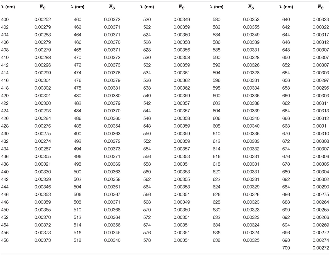
Table A1. Normalized spectra [${\overline{E}}_S(\lambda )$, dimensionless] for the visible spectra (400–700 nm).