Internal Wave Observations Off Saba Bank

Introduction

Saba Bank in the Caribbean Netherlands is the largest submarine atoll in the Atlantic Ocean. It rises about 1000 m above the surrounding sea floor and it has a total surface area of approximately 2200 km² of which 1600 km² is shallower than 50 m (van der Land, 1977). This rather flat top of the bank (Figure 1) and especially its adjacent fringes on the east and the southeastern flanks are known for the presence of a teeming tropical coral community and associated marine life between 7 and 15 m water depth, which have been the focus of many recent studies (e.g., McKenna and Etnoyer, 2010; de Bakker et al., 2016). By contrast, very little is known about marine life and the physical-chemical environmental conditions of the deeper (> 50 m) parts of Saba Bank including its slopes. In this paper we present water column observations along transects and more detailed mooring observations of currents and especially temperature that describe the physical environment between 250 and 500 m from the north and south slopes of Saba Bank. Both slopes have their own characteristics, which demonstrate a contrasting setting, the southern slope being steeper than the northern slope.

FIGURE 1

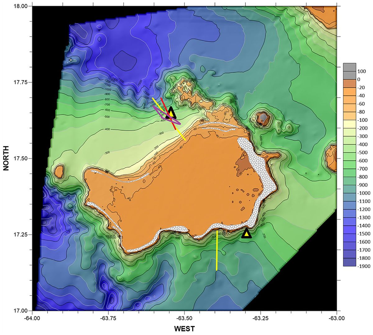
Figure 1. Saba Bank topography from GEBCO data, with mooring locations at the two triangles to the North (MN) and South (MS) of the Bank. Saba island is visible in gray to the northeast of the Bank. The tidal current ellipses near MN are the mean values for the upper (red) and lower (purple) 50 m of the ADCP good-data range. The length of the red rectilinear ellipse is 0.06 m s^-1. The yellow lines indicate CTD-transects. The dotted areas coarsely indicate the location of coral reefs, drawn after (van der Land, 1977).

Observations above seamounts and raised atolls in other ocean areas showed that motions in the ocean interior are important for the replenishment of oxygen and nutrients to deep-sea organisms ranging from microbes to corals and sponges. An example is the breaking of internal waves on steep sloping sides of underwater mounts influencing cold-water coral reef growth (e.g., Genin et al., 1986; Wang et al., 2007; Chen et al., 2016; Cyr et al., 2016; van Haren et al., 2017). The generally stable density stratification in the ocean, a result of the dominant solar insolation storing large amounts of potential energy, hinders but does not prevent the vertical diapycnal exchange of suspended and dissolved matter. This is because the relatively modest kinetic energy input via atmospheric disturbances in combination with the Earth rotation and tides sets the stratification in motion. The resulting internal waves are not only generated via interaction with abundant underwater topography, but also dissipate their energy via turbulent breaking mainly at relatively steep sides, just steeper than those of internal tides (van Haren et al., 2015; Winters, 2015; Sarkar and Scotti, 2017). This is considered (Stigebrandt, 1976; Eriksen, 1982; Thorpe, 1987) the dominant generator of turbulence in the ocean, without which most deep-sea life would come to a halt.

With many Caribbean coral reefs in decline (Burke and Maidens, 2004; Hoegh-Guldberg et al., 2007) the extensive and relatively viable coral reef of Saba Bank urgently summons for studies on how to preserve this unique natural heritage. Especially since Saba Bank may act as buffer and resource of larvae for other Caribbean reef habitats. Considering the importance of ocean-reef interactions for sustenance of coral communities, the lack of information on Saba Bank hydrography and interactions with the surrounding ocean must be solved with priority. In the framework of the Netherlands Initiative Changing Oceans ‘NICO’ Saba Bank was visited with RV Pelagia in February 2018 during the Caribbean ‘winter’ period, when trade winds blew near the surface, while passages of hurricanes did not occur. The observations presented in this paper focus on turbulence and internal wave structure by means of high-resolution temperature sensor moorings. They demonstrate some unique findings compared with other ocean topography areas.

Materials and Methods

For about 23 days two identical taut-wire moorings were deployed around 500 m water depth at the north and south slopes of Saba Bank in the Caribbean Sea (Figure 1). The two deployment sites were selected to represent the principal slope habitats on Saba Bank, i.e., its gently rising northern slope, which is not connected with the shallow water reef, versus its abruptly rising southern slope, which relates to the reef community on its shallow top (Bos et al., 2016).

Prior to deployment of the moorings, extensive shipborne Sea-Bird 911plus Conductivity Temperature Depth CTD profiles were made. The CTD package also included an SBE43 dissolved O₂ sensor, a Wetlabs FLNTU combined turbidity/fluorescence sensor, and a Wetlabs C-star transmissometer. For water sampling at selected depths, 24 Niskin bottles of 12 L were mounted. Two CTD transects were carried out from the shallow bank toward deeper water with stations situated 1800 m apart horizontally (Figure 1). For the analysis of inorganic nutrient concentrations (phosphate, nitrate, nitrite) water samples were filtered on board through 0.2 μm polycarbonate membrane filters (Whatman Nuclepore) and vials were stored frozen at -20°C. Nutrient concentrations were determined by colorimetric analyses on board using a QuAAtro Continuous Segmented Flow Analyzer (Seal Analytical Ltd., United Kingdom). All measurements were calibrated against standards diluted to known nutrient concentrations with low nutrient seawater. Each run of the system produced a calibration curve with a correlation coefficient of at least 0.9999 for 10 calibration points, but typically 1.0000 for linear chemistry. A freshly diluted, mixed nutrient standard, containing silicate, phosphate, and nitrate, was measured in every run, as a guide to monitor the performance of the standards. To measure the precision at different concentration levels, standards of different concentrations were each measured six times. For PO4 the standard deviation was 0.003 at a concentration level of 0.6 μM/l, for NO3 the standard deviation was 0.04 at a concentration level of 8 μM/l and for NO2 the standard deviation was 0.001 at a concentration level of 0.2 μM/l.

The two moorings were named according to their position relative to the Bank as mooring south ‘MS’ and mooring north ‘MN’. Between 12 UTC on 14/02/18 and 13 UTC on 10/03/18, MN was deployed at 17° 38.90′N, 63° 32.68′W, H = 483 m water depth. This site had a relatively small bottom slope angle, computed on 1 km horizontal scales,of β = 3.6 ± 0.5°. About 7 km to its northeast a shallow promontory, Luymes Bank was situated. Between 19 UTC on 15/02/18 and 18 UTC on 09/03/18, mooring South ‘MS’ was deployed at 17° 15.62′N, 63° 17.89′W, H = 493 m, with relatively steep β = 10.8 ± 0.5°.

The slope angle γ(σ, N) = sin^-1[((σ²-f²)/(N²-f²))^1/2] (e.g., LeBlond and Mysak, 1978) of free internal wave propagation was computed for wave frequency σ and large-scale mean buoyancy frequency N ≈ 5 × 10^-3 s^-1 at local latitude inertial frequency f ≈ 4.5 × 10^-5 s^-1. Under local conditions the semidiurnal slope is γ(M₂, N) ≈ 1.6° and both mooring sites have a bottom slope β > γ(M₂), super-critical for internal tides. Thus, freely propagating internal waves have periods between about 1.6 days (inertial period) and 1200 s (mean buoyancy period), including diurnal and semi-diurnal tides. As will be demonstrated in Section 3, the internal wave band varied locally as under the weakest stratification in internal-wave-strained small areas of 10–50 m high and several hours in duration N_min ≈ 6 × 10^-4 s^-1, which provides a buoyancy period of about 3 h. Under strong stratification in thin layers of <10 m thick the internal wave band is stretched to N_max ≈ 1.5 × 10^-2 s^-1, which provides a buoyancy period of about 400 s.

Each mooring consisted of a heavy top-buoy providing 2900 N (290 kg) net buoyancy with a downward looking 75 kHz acoustic Doppler current profiler ‘ADCP’ at about 350 ‘mab’, meters above the bottom. The ADCP sampled all three Cartesian current components [u v w] in 70 vertical bins of 5 m, storing ensemble data every 120 s. Due to the acoustic beam spread at 20°-angles from the vertical, the current components represent horizontal averages over 20–240 m diameter circles. The tilt and pressure sensors demonstrated that the top-buoys did not move more than 0.15 m vertically and not more than 10 m horizontally, under maximum current speeds of about 0.4 m s^-1.

Between 5 and 245 mab 121 ‘NIOZ4’ (van Haren, 2018) self-contained high-resolution temperature (T) sensors were attached to a 0.0063 m diameter plastic-coated steel cable at 2.0 m intervals. The T-sensors ranged the lower half of the local water column and sampled at a rate of 1 Hz with a precision of < 0.5 mK and a noise level of < 0.1 mK. For typical current speeds of 0.1 m s^-1, the 1-Hz sampling represents a 0.1 m horizontal scale resolution. The T-sensor data thus have a 100–1000 times better resolution of internal wave – turbulence characteristics than the ADCP-data. In this paper, the moored T-sensors provide the primary data-set, with the secondary ADCP support on current information. At MN, six sensors showed various electronic (noise, calibration) problems and were not further considered in this study, while their data were interpolated. At MS, data from 9 T-sensors were interpolated. The T-sensors were synchronized via induction every 4 h. Thus, each 240-m vertical profile was measured in < 0.02 s.

The moored observations were supported by the shipborne CTD-data to establish a, preferably linear, temperature-density relationship to be able to compute turbulence parameter estimates from the moored T-sensor observations. This is because in the ocean temperature and salinity can contribute significantly to variations in potential density anomaly, referenced to the surface, σ_𝜃 = ρ – 1000 + pressure effects. Only unstable σ_𝜃(z,t) establish turbulent overturning. To this end, turbulence parameter estimates were obtained using the moored T-sensor data as proxies for density variations by calculating ‘overturning’ scales. These scales followed after reordering (sorting) the 240 m high profile σ_𝜃(z) every 1 s, which may contain inversions, into a stable monotonic profile σ_𝜃(z_s) without inversions (Thorpe, 1977). After comparing observed and reordered profiles, displacements d = min(|z-z_s|).sgn(z-z_s) were calculated necessary for generating the reordered stable profile. Tests applied to disregard apparent displacements associated with instrumental noise and post-calibration errors (Galbraith and Kelley, 1996). Such a test-threshold is very low for NIOZ-temperature sensor data, < 5 × 10^-4∘C (van Haren, 2018). Then the turbulence dissipation rate was calculated following,

$\text{ε}=L_O{}^2{N}^3=0.64d^2{N}^3,\mathrm{\left(}\mathrm{1}\mathrm{\right)}$

where N denotes the buoyancy frequency computed from each of the reordered, essentially statically stable, vertical density profiles. L_O denotes the Ozmidov-scale of largest overturns in a stratified fluid. The numerical constant followed from the mean of the outcome of empirically relating many ocean-observed overturning scales with Ozmidov-scales: L_O = 0.8d (Dillon, 1982). Vertical turbulent diffusivity K_z = Γ𝜀N^-2 was computed whereby a constant mixing efficiency of Γ = 0.2 was established for oceanographic, not laboratory, observations (Osborn, 1980; Oakey, 1982; Gregg et al., 2018) as a mean value for the conversion of kinetic into potential energy, so that,

$K_{\text{Z}}=0.128d^{2}N.\mathrm{\left(}\mathrm{2}\mathrm{\right)}$

We calculated non-averaged d in (1) for displaying high-resolution distributions of 𝜀(z, t). For general use, we calculated ‘mean’ turbulence parameter values by averaging original (1) and (2) data in the vertical [ ], in time <>, or both. The 1-Hz sampling of moored T-sensor data allowed sufficient averaging over all different turbulence characteristics.

The errors in the mean turbulence parameter estimates thus obtained depended on the error in N, and the error in the temperature-density relationship, since the instrumental noise error of the T-sensors was negligible. Given the errors, the estimated uncertainty in time-depth mean estimates of (1) and (2) amounted about a factor of 2. Using similar T-sensor data from Great Meteor Seamount, van Haren and Gostiaux (2012) found turbulence parameter estimate values to within a factor of two similar to those inferred from ship-borne CTD/Lowered-ADCP data near the bottom.

Observations

CTD Transects

Measurements along each CTD-transect were made sequentially, i.e., within a period of about 18 h. On both flanks of Saba Bank a well stratified water column was found below a near-homogeneous upper layer and a distinct pycnocline between -80 and -100 m (Figure 2A). Beam transmission (Figure 2B) showed a marked dip around the pycnocline (where a fluorescence peak was found, not shown). On both flanks a broad oxygen minimum of about 120 μmol kg^-1 was found between -400 and -700 m (Figure 2C). Near the surface, values around 210 μmol kg^-1 were observed. In the -700 to -400 m depth-range highest inorganic nutrient values were found (Figure 3). In contrast, the near-homogeneous upper layer was depleted of inorganic nutrients. No clear differences in dissolved nutrient concentrations were observed between the northern and southern flanks.

FIGURE 2

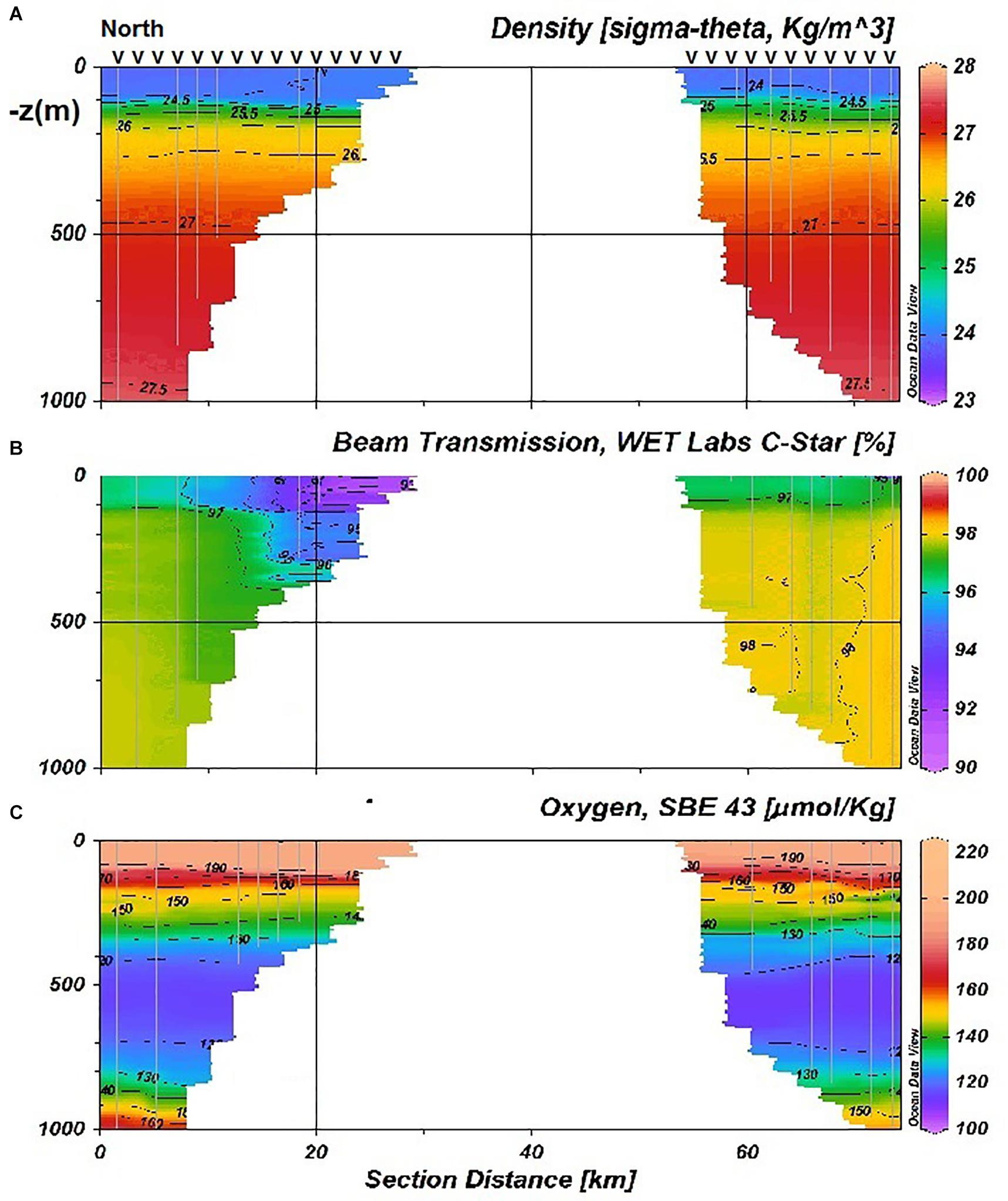
Figure 2. Cross section of the water column along CTD-transects to the north and south of Saba Bank. North is to the left. The tick-marks indicate the stations. (A) Density anomaly referenced to the surface. (B) Beam transmission. (C) Oxygen content.

FIGURE 3

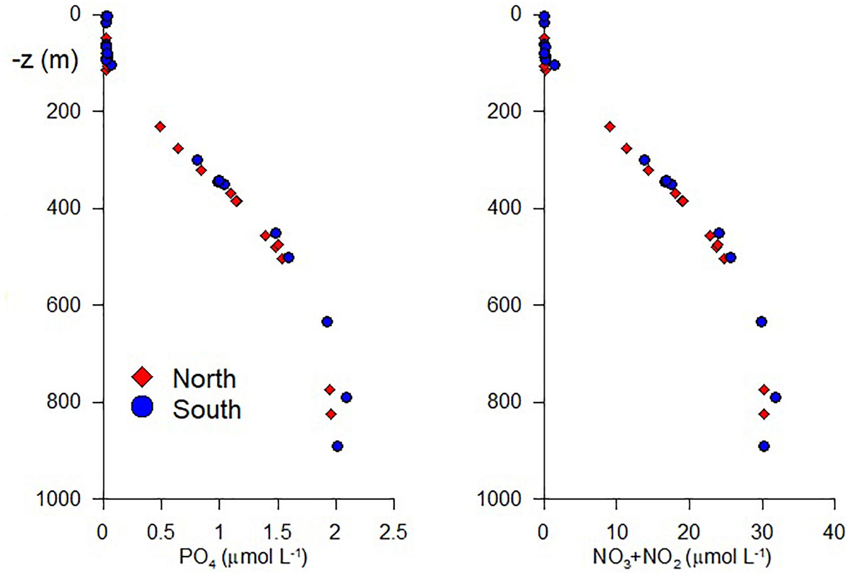
Figure 3. Vertical profiles of inorganic dissolved nutrient concentrations of all CTD stations collated along the northern and southern flanks.

The most conspicuous difference between the two transects was the lower temperature in combination with the enhanced turbidity (lower beam transmission) over the shallow part of the northern transect slope, especially near the perimeter of Saba Bank. Turbidity was elevated also further down the northern slope to -500 m. Fluorescence was slightly elevated in the upper water column above the northern slope but did not match the more extensive turbidity maximum (not shown).

Moorings

The CTD-profiles at the two mooring sites revealed that the gradual decrease of Conservative (∼potential) Temperature Θ (Intergovernmental Oceanographic Commission [IOC] et al., 2010) with depth below the near-homogeneous near-surface layer showed numerous small-scale wiggles or steps (Figure 4A). In the same depth range, Absolute Salinity (Figure 4B) first increased with depth, down to about -130 m thereby dominating density variations, and subsequently decreased further down, showing similar small-scale steps as Θ. Its decrease with depth implied that salinity partially counteracts temperature in density variations (Figure 4C).

FIGURE 4

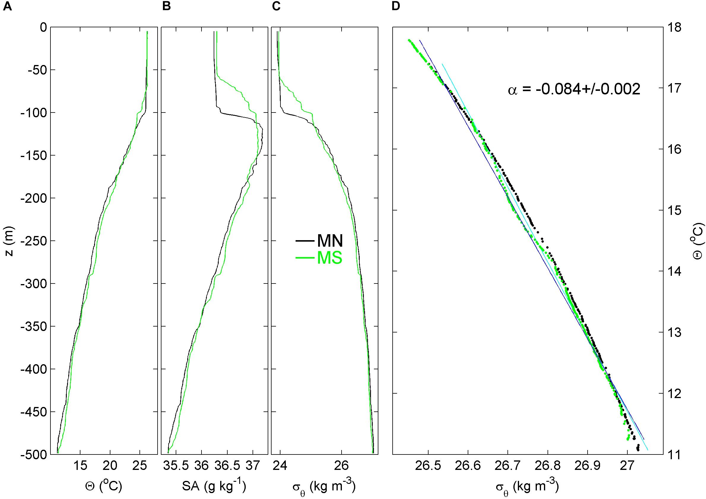
Figure 4. CTD-profiles to within 1 km from MN (black) and MS (green). (A) Conservative (∼potential) Temperature. (B) Absolute Salinity. (C) Density anomaly referenced to the surface. (D) Conservative Temperature-density anomaly relationship, from the CTD-data between 250 and 500 m, with mean linear fit indicated in numbers.

Over the range of moored T-sensor observations between about -250 and -500 m, variations in σ_𝜃 followed a reasonably tight relationship with Θ, δσ_𝜃 = αδΘ, where α = -0.084 ± 0.002 kg m^-3∘C^-1 denotes the effective thermal expansion coefficient under local conditions over the range of T-sensors (Figure 4D). The relationship deviated somewhat from a linear fit because of the slightly varying contribution of salinity with depth.

The rather strong stratification with depth over the range of T-sensor observations was reflected in the time-depth series of observations at the two mooring sites (Figure 5). Overall as well as the mean at any given depth, Θ was slightly higher at MN than at MS. Both sites showed a dominant tidal variability with amplitudes far exceeding the surface tidal range of about 1 m. The internal tides displayed mainly semi-diurnal variation with a diurnal modulation especially at MN. However, the sites showed a very distinct semidiurnal internal tide difference with depth which is best visible by comparing the isotherm patterns. At MN, internal tide amplitudes were typically 50 m crest-trough but have a rather strong non-uniformity or large phase variation over the vertical range of observations: These waves appeared in quasi ‘mode-2,’ second baroclinic mode, over a vertical range of about 150 m across which the motions are approximately 180° out-of-phase. It is noted that the decomposition into vertical modes is not valid over sloping topography (e.g., LeBlond and Mysak, 1978), hence the addition ‘quasi’ is applied here. At MS, the amplitudes varied more rapidly with time, with a modulation between 3 and 10 days, up to 100 m crest-trough and they were more or less uniform with little phase variation over the vertical range of observations: Quasi-mode-1, first baroclinic mode.

FIGURE 5

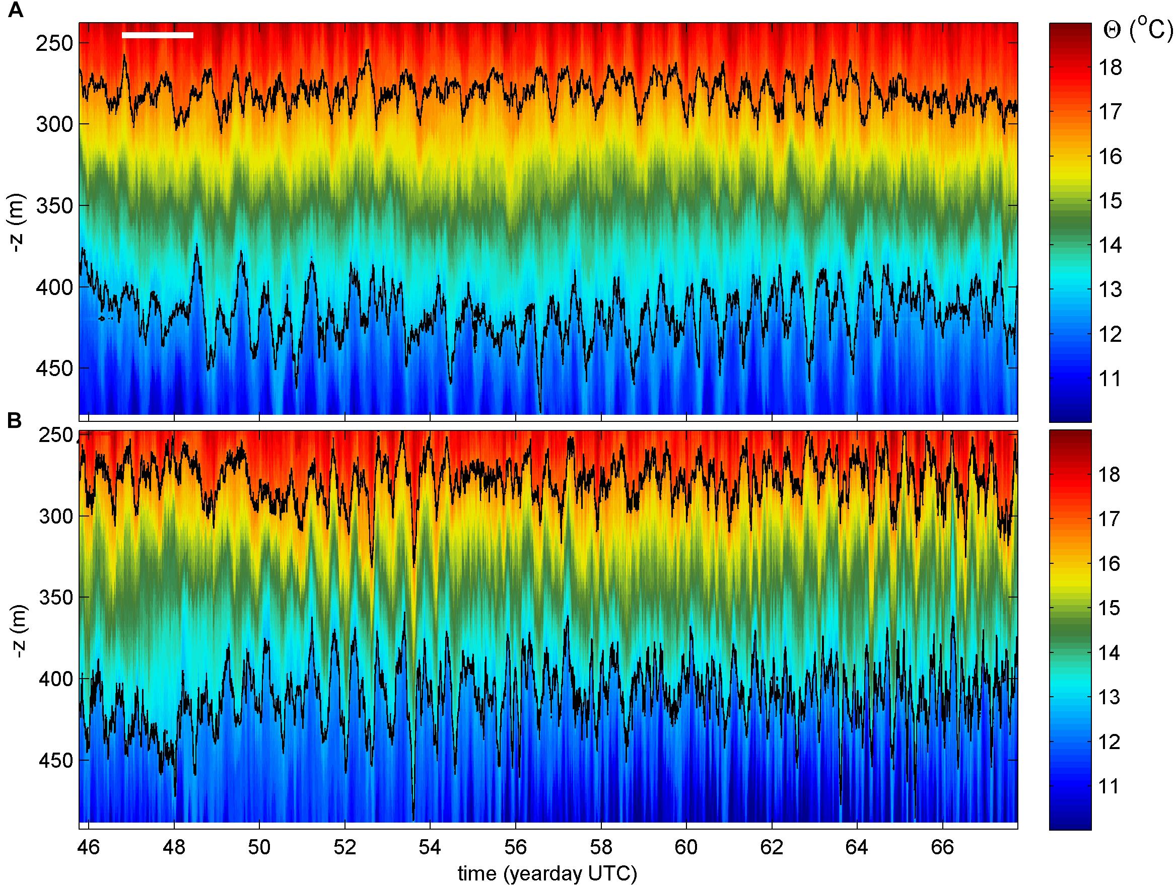
Figure 5. Depth-time overview of Conservative Temperature from moored high-resolution T-sensors, with missing sensors interpolated (see text). The time range is common for both moorings and the local bottoms are at the horizontal axes. The black contours are for 12.7 and 16.7°C. (A) MN. The white horizontal bar indicates the local inertial period. (B) MS. Time here and all other plots is in UTC.

Three-week mean cross-spectra between all possible pairs of T-sensors at vertical separation distances of Δz = 8 and 160 m demonstrated the different vertical phase structure between the two mooring sites (Figure 6). For Δz = 8 m, coherence level ‘coh-lev’ was significantly different from noise for σ < 12 cycles per day ‘cpd’ ≈1.6 N, at both MN and MS. Corresponding phases, which are only meaningful for coh-lev > ∼0.19, were strictly zero throughout this frequency-range. The only difference between MN and MS was the slightly higher coh-lev at tidal harmonic fourth- and sixth-diurnal frequencies at MS. In contrast for Δz = 160 m, only at MN and only at semidiurnal frequency (incl. lunar M₂) large coh-lev was found. The corresponding phase (difference) is |180°|± 10° (Figure 6B). At MS, coh-lev was significant but weak at M₂ at Δz = 160 m, with a phase of 0 ± 10° (Figure 6D). The remainder of the internal wave band showed some coherence at tidal harmonics, for MS only with phases of |50°|± 10°. The portion N_min < σ < N showed no significant coh-lev and erratic phases. It is noted that at both sites a weakly significant coh-lev was still found around N, with a phase of 0 ± 30°.

FIGURE 6

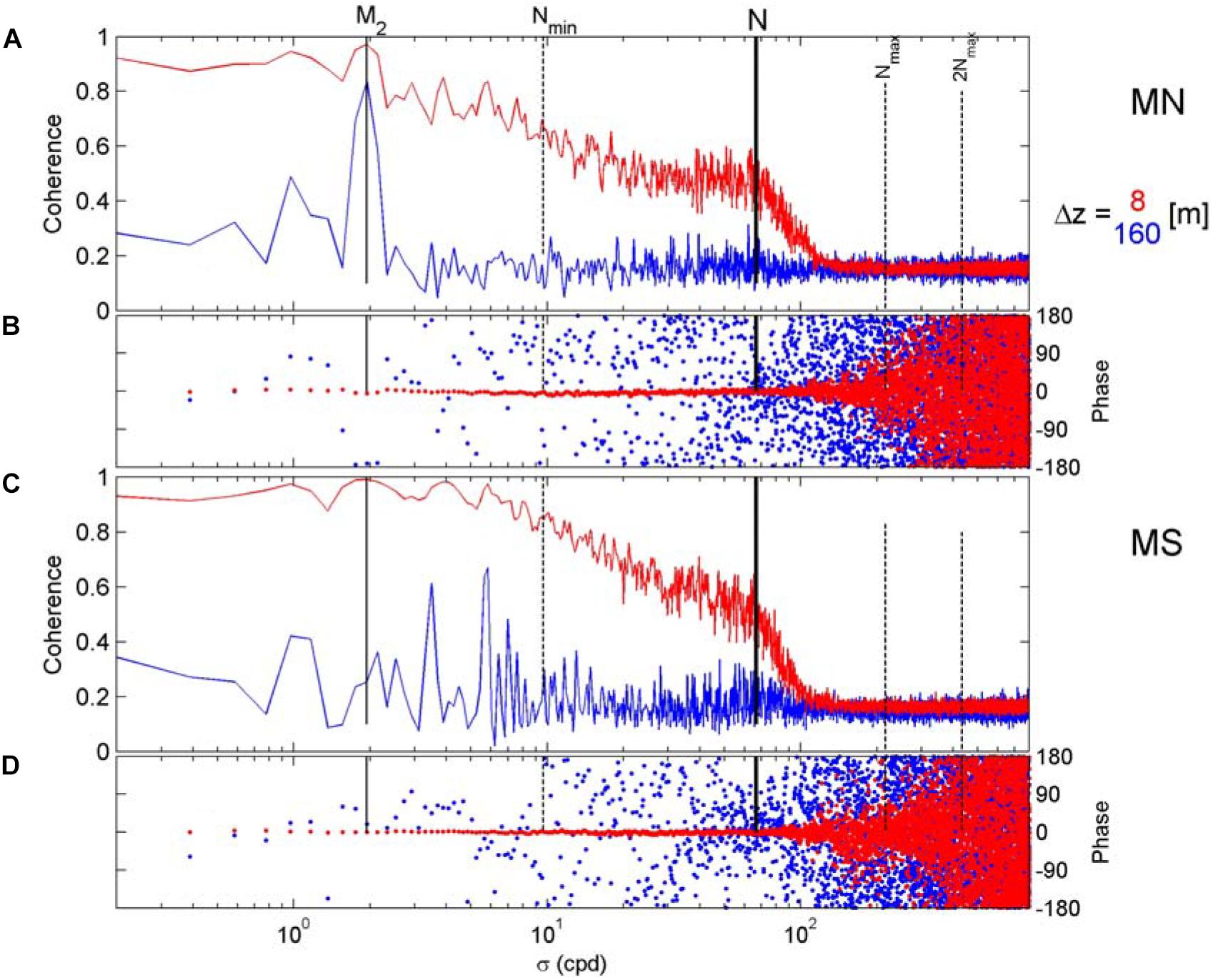
Figure 6. Strongly smoothed (∼400 degrees of freedom ‘dof’) three-week mean cross-spectral coherence and phase between all possible non-overlapping pairs of T-sensors vertically separated by 8 m (red) and 160 m (blue). The focus is on the [f, N] range, with particular frequencies indicated. N_min indicates the overall minimum buoyancy frequency, N_max indicates the maximum small-, 2 m, scale buoyancy frequency. (A) MN coherence ‘coh-lev’. The 95% significance level coh-lev ≈ 0.19. (B) MN phase, with relevant values only for coh-lev > 0.19. (C) MS coherence. (D) MS phase.

The difference in vertical semidiurnal tidal phase structure between MN and MS is also observed in three-week mean spectra (Figure 7). While the semidiurnal temperature difference ΔΘ peaks at MN larger than Θ, the semidiurnal temperature Θ peaked higher than ΔΘ together with higher harmonics up to minimum buoyancy frequency N_min at MS. Outside the tidal frequencies, the spectral slope σ^-1 (‘-1’ on a log-log scale) of ocean interior non-breaking internal waves (van Haren and Gostiaux, 2009) was found over a short range f < σ < M₄ and also close to N, N/2 < σ < N at MN. For MS, the -1-slope was found at the base of the tidal harmonics for f < σ < N_min.

FIGURE 7

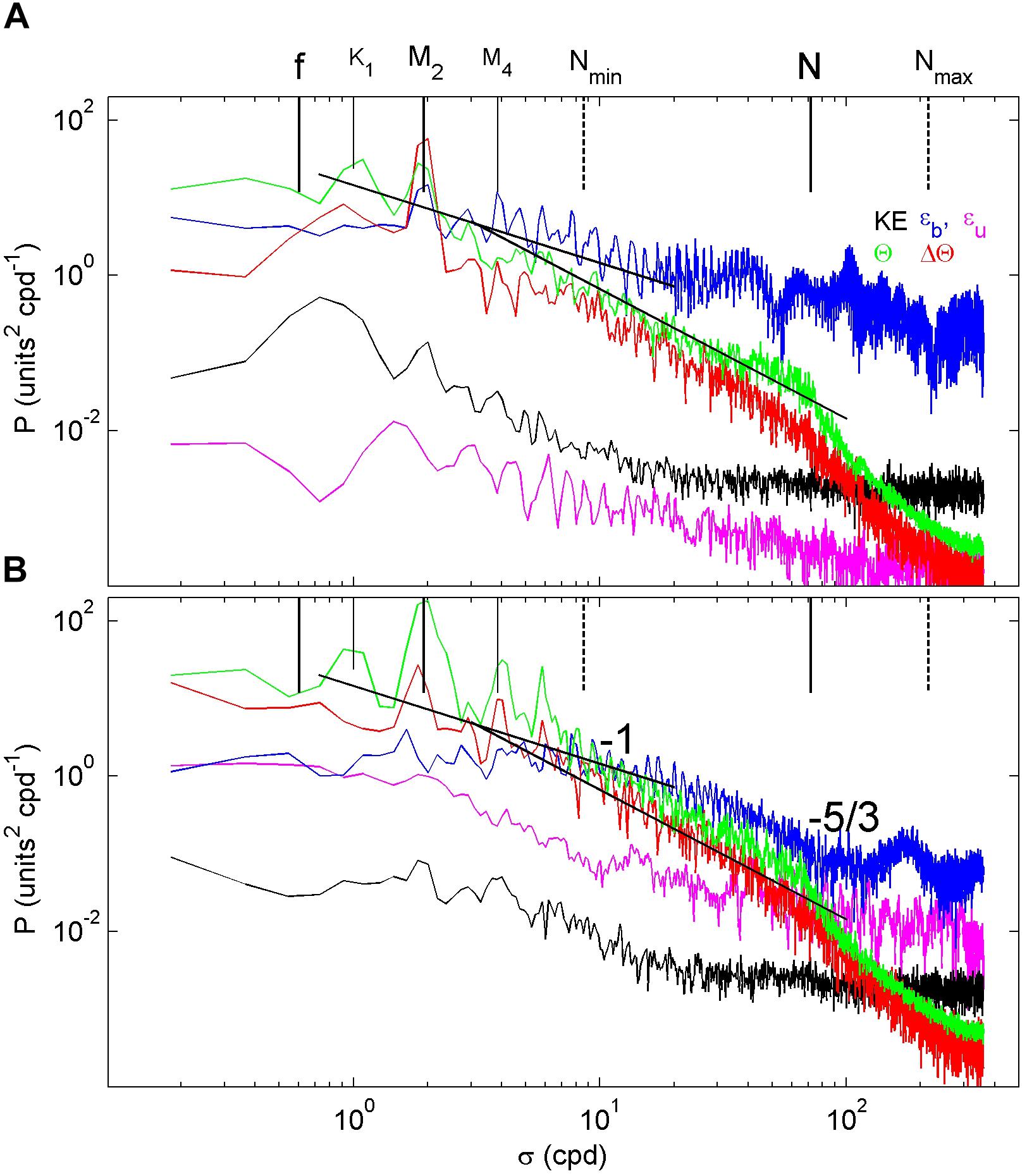
Figure 7. Weakly smoothed 10 dof entire mooring period spectra of 120 s common (sub-)sampling from ADCP and T-sensor data for: Conservative Temperature at –365 m (green; average over 10 sensors between –355 and –375 m), T-difference between –325 and –405 m (red), kinetic energy (with similar form as the shear spectrum) at –335 m (black), dissipation rates averaged over lower 60 m between –427 and –487 m = 5 mab (blue) and over the upper 60 m (purple). For reference spectral slopes are indicated in black lines. (A) MN. (B) MS, with legend for spectral slopes like ‘–1’ implying P(σ) ∝ σ^-1.

The range of M₄ < σ < N/2 sloped at -5/3, which reflects a mean dominance of shear-induced turbulence or a passive scalar (Tennekes and Lumley, 1972). Here the Taylor hypothesis is invoked and verified using the ADCP-data and the method by Pinton and Labbé (1994) for non-steady currents. Like for Atlantic seamount T-sensor data (Cimatoribus and van Haren, 2015), the data-transfer from time to horizontal space domain hardly mattered for its spectral slopes. The wavenumber spectra even showed a slightly tighter -5/3-slope, at the expense of a lower resolution by a factor of about 4 (= maximum/mean current speed ratio). Thus and for comparison with cross-spectra we present frequency spectra only.

The -5/3-slope ‘inertial subrange’ is commonly observed outside the internal wave band at higher frequencies N < σ < 4N_max, for example in intense internal wave breaking above a large seamount slope and a biologically rich seamount (Cimatoribus and van Haren, 2015; van Haren et al., 2017). It is noted that in the latter the -5/3-slope extends in the internal wave range but for a small fraction around 10 cpd. In the present observations from MS, this -5/3-slope was observed throughout the ‘internal wave’ range portion N_min < σ < N, with a much steeper slope less than -3 for N < σ < N_max and -2 for σ > >N_max (Figure 8A). The latter reflects fine-structure contamination or convective turbulence (active scalar). In the present inertial subrange the T-variance was somewhat larger at MS than at MN. In this range, coh-lev behaved as common for an open-ocean internal wave band (cf. van Haren and Gostiaux, 2009), including a fast drop-off into non-significant coh-lev at or just above N (Figure 8B). This contrasts strongly with a gradual decrease from N to 3N_max observed over a seamount (van Haren et al., 2017). In fact, the present coh-lev decrease already starts away from near-1 at N_min (Figure 8B).

FIGURE 8

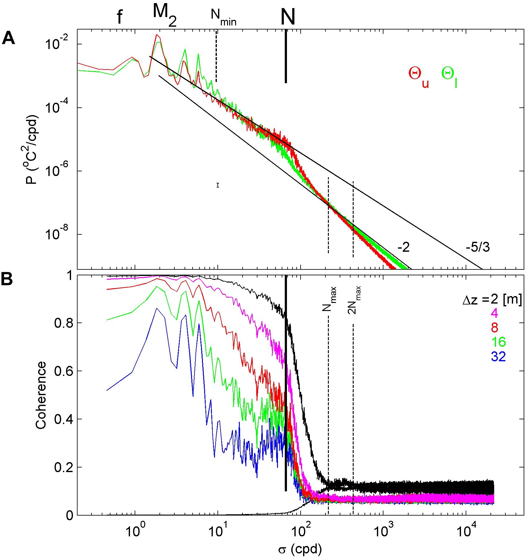
Figure 8. Spectral comparison of moored T-observations from MS. (A) Power spectra, heavily smoothed ∼1000 dof for upper 50 (red) and lower 50 sensors (green). (B) Coherence level between all possible non-overlapping pairs of T-sensors, over vertical distances as given. The 95% confidence level is indicated by the dashed line for Δz < 2 m near the bottom (always coh lev < 0.16). N_max here also marks where coh-lev first drops into noise.

The associated turbulence dissipation rates were found slightly larger at MN than at MS for the lower 5–65 mab. This time series’ spectrum was elevated at tidal frequencies for MN, and rolled off for σ > N_min at both moorings (Figure 7). For σ > N it leveled off, with a small sub-peak near N_max for MS. Between upper 185 and 245 mab, turbulence parameter values were half (MS) to one (MN) order of magnitude lower than near the bottom. When averaged over the entire mooring period of 21 days and over the range of sensors between 5 and 245 mab these turbulence parameter values amounted for MN: <[𝜀]> = 3.8 ± 2.5 × 10^-8 m² s^-3 and <[K_z]> = 6.8 ± 4 × 10^-4 m² s^-1, while <[N]> = 4.9 ± 1 × 10^-3 s^-1. For MS they were: <[𝜀]> = 5.1 ± 2.5 × 10^-8 m² s^-3 and <[K_z]> = 9 ± 5 × 10^-4 m² s^-1, while <[N]> = 4.9 ± 1 × 10^-3 s^-1. These mean values were similar within the error bounds. Mean near-bottom values were twice the overall mean values.

The difference in near-bottom dissipation rate time series partially reflected the difference in ADCP-observed kinetic energy (and shear, not shown). At MN mid-range (-330 m), a large broad peak in kinetic energy was observed at just super-inertial frequency and extending toward diurnal frequencies (Figure 7). This broad peak was absent in the kinetic energy spectrum from MS, which was otherwise similar with small peaks at semidiurnal and higher harmonics, leveling off into noise for σ > N_min. This difference between the currents implied a strong influence of near-inertial motions at MN where quasi-mode-2 internal tides were observed in Θ. There, mean semidiurnal current ellipses showed a long axis amplitude decrease from 0.06 m s^-1 around -250 m 0.04 m s^-1 around -450 m, with a direction more or less perpendicular to the isobaths (Figure 1).

Magnifications

A magnification of 1 day of data showed the asymmetry of the internal tide between the two sites (Figure 9 for MN, Figure 10 for MS). The quasi-mode-2 at MN is quite distinct in Figure 9, with a dominant near-bottom turbulent overturning when the wide-strained isopycnals reach the bottom. This straining took a full tidal period. It was not a quasi-mode-2 high-, near-buoyancy-frequency internal wave packet occurring once every 12 h. Wide-straining and associated overturning also occurred in the interior with periods of prolonged overturning lasting shorter than the minimum buoyancy period and up to the local maximum buoyancy period. This may be verified by comparing the sizes of non-zero dissipation rate patches in Figure 9C with the time-scales in Figure 9A. When apparent overturning lasts longer than the local (maximum) buoyancy period it may reflect lateral, partially salinity-compensated intrusions. The observed overturning shapes did not indicate intrusions, which confirmed the CTD-profiling below z < -200 m (Figure 4).

FIGURE 9

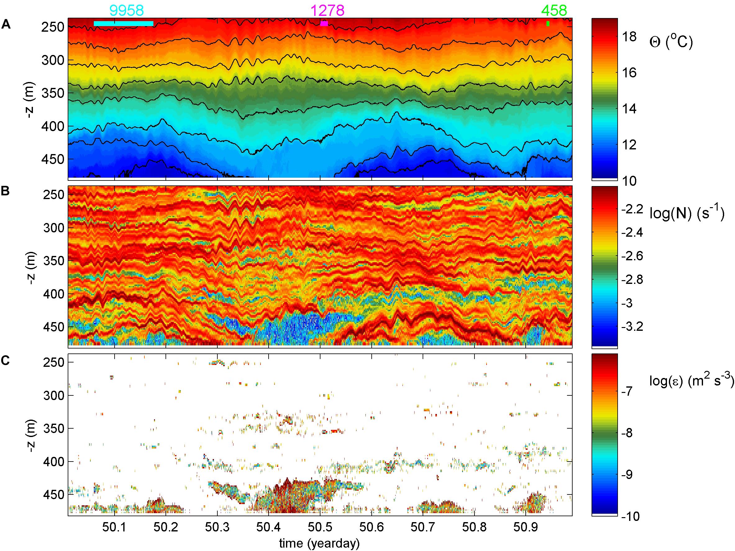
Figure 9. One day detail from Figure 5A, MN. (A) Conservative Temperature. Black contours are drawn every 1.0°C. The horizontal bars indicate from left to right maximum (light-blue), mean (purple) and minimum (green) buoyancy periods. (B) Logarithm of buoyancy frequency per vertical increment and per time step. (C) Logarithm of dissipation rate.

FIGURE 10

Figure 10. As Figure 9 withidentical ranges, but for Figure 5B, MS.

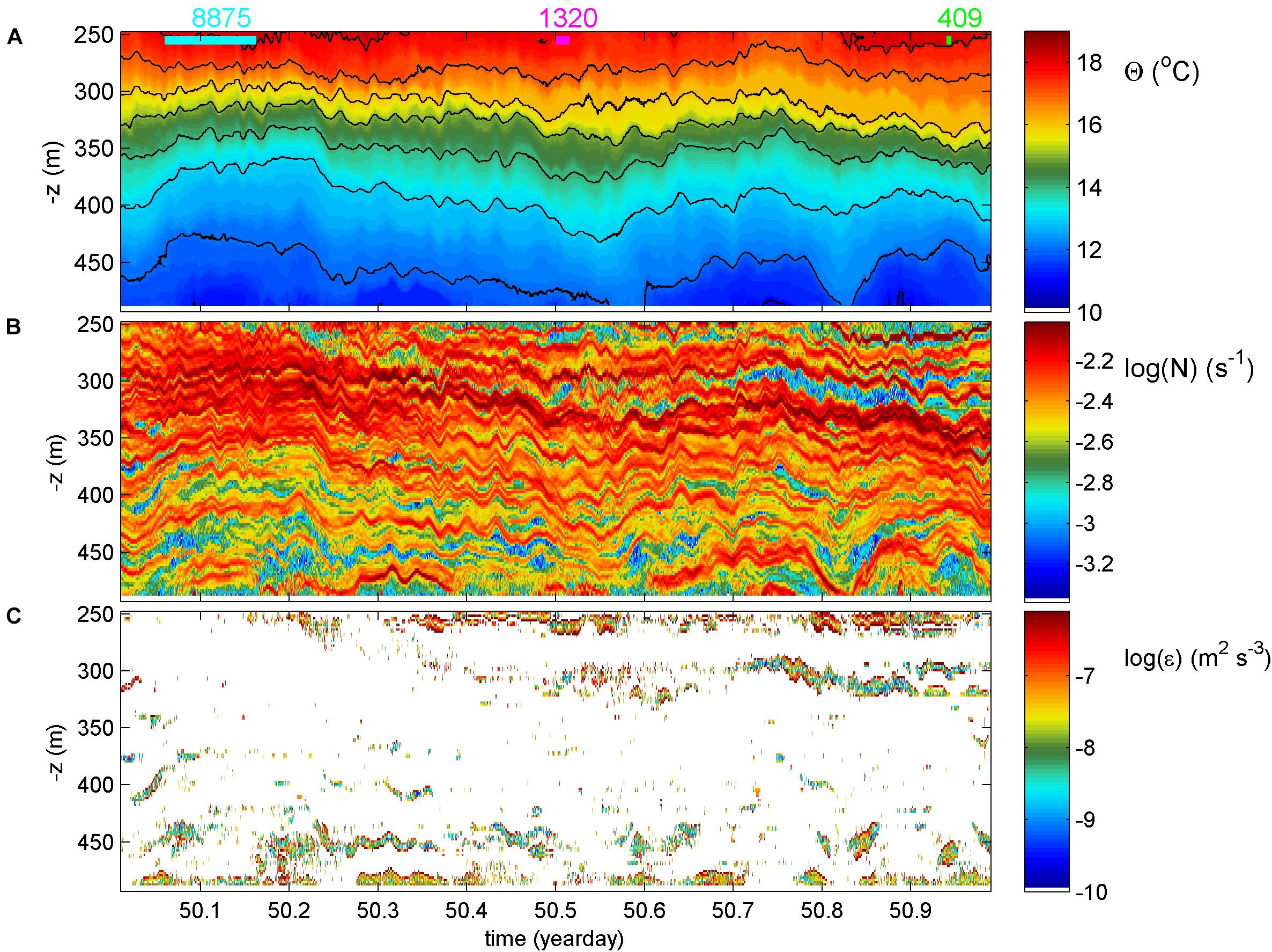
While turbulent overturning seemed larger near the bottom at MN (Figure 9B), it was found throughout and particularly also near the top of the range at MS (Figure 10). At both moorings, the abundant layering of alternating strong and weak stratification confirmed the many steps in the CTD-profiles. The layering was seen to episodically reach the lowest sensors at 5 mab, and a near-homogeneous bottom boundary layer was never observed for any prolonged period of time like the tidal period or 1/f ≈ 6.3 h. At neither of the mooring sites non-linear frontal bores were observed close to the bottom.

The absence of frontal bores is visible in the magnifications of the lower 60 mab around times of relatively strong turbulent overturning (Figure 11). While high-frequency internal waves with periods close to the mean buoyancy period and up to the local maximum buoyancy period were at the interface, no front was seen steepening from the bottom near-vertically upward. Moreover, turbulent overturning in the core behind the front did not resemble a backward breaking wave. Nevertheless, the obviously erratic motions provide a local T-spectrum that has an inertial subrange extending beyond σ > N (not shown). These examples were not associated with periods of transition from warming to cooling carrier (tidal) waves. It is noted that such transition phases were not found particularly turbulent, see also Figure 11A around day 50.5 and the associated small near-bottom turbulence dissipation rate in Figure 9C.

FIGURE 11

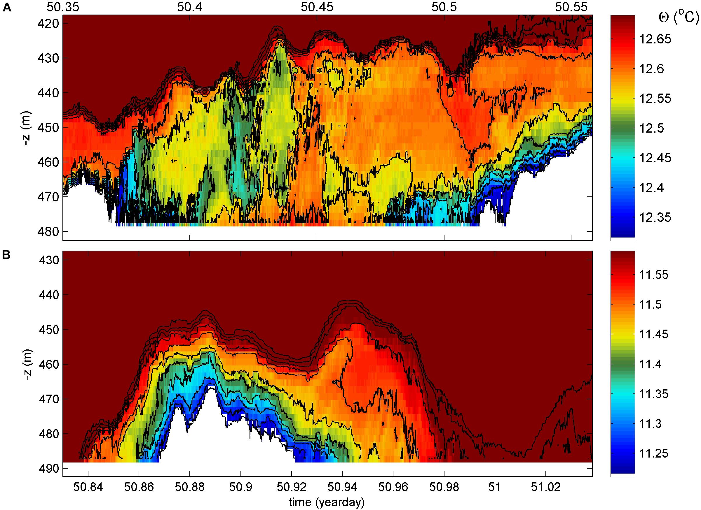
Figure 11. Five hour near-bottom details of Figure 5, with different color ranges and contours every 0.05°C. (A) MN. (B) MS.

Discussion

The Caribbean Sea around Saba Bank was found to be vertically well stratified in temperature and density below the photic zone. The stratification supported a large range of internal waves with excursions of 50–100 m, crest-trough. The waves set the sea interior in constant motion, whereby the stratification was not smooth but highly layered with alternating strong and relatively weak stratification every 5–50 m vertically, while lasting up to 3 h. This varying layering was due to straining by internal waves at multiple scales that might break occasionally after being induced by current-shear. These observations seemed highly comparable with those from the upper 400 m in the open West-Pacific, at 30 km off the Californian coast in 1500 m water depth (Alford and Pinkel, 2000). However, at the latter site the straining internal wave field generated mean turbulence values of nearly one order of magnitude smaller than observed here. Further out into the open-ocean, turbulence values tend to be another order of magnitude smaller (Gregg, 1989) whereas the internal wave band spectrum shows a smooth -1 slope (van Haren and Gostiaux, 2009). In the present observations the background spectrum pointed at a dominance of shear-induced turbulence inside this band outside tidal harmonic frequencies.

The present observations appeared also anomalous in comparison with data from sites above large-scale topography in the Atlantic Ocean and elsewhere. Whilst the slopes at the mooring sites north and south of Saba Bank were rather steep and on all accounts were supercritical for internal tides for given stratification, no highly non-linear upslope propagating bores were observed in the three-week records. This might explain the weaker overall mean turbulence by about a factor of two than found above Great Meteor Seamount ‘GMS’ where bores did occur at comparable depth and whirled up sediment several tens of meters away from the bottom (van Haren and Gostiaux, 2012). While above GMS and other areas with sloping topography the inertial subrange of shear-induced turbulence dominated the several weeks temperature spectrum at frequencies > N, it was only dominant in the internal wave band < N above Saba Bank slopes. More specifically, it dominated between N_min and N here, which suggested that local minimum-N sets the internal wave limit while mean-N sets the shear-turbulence overturning limit. Apparently for σ > N, either interfacial layer advected passed the sensors (‘fine-structure contamination’) were more dominant or convective (active scalar) turbulence. The sites show more open-ocean than sloping topography internal wave-induced turbulence, albeit at much higher levels than actually found in the open ocean.

As in areas where non-linear bores dominate near-bottom mixing, the present internal wave breaking reached the bottom, especially in the quasi-mode-2 internal tide fashion for MN, and dominated over possible frictional flow turbulence. The latter, commonly termed ‘Ekman dynamics’ after Ekman (1905) does not reach higher up than about 10 mab for given flow speed, and is considered to leave behind a near-homogeneous layer above the sea floor. As stratification was observed to reach the lowest T-sensor at 5 mab, and in previous observations to 0.5 mab (van Haren and Gostiaux, 2012), the internal waves not only dominated turbulent overturning but also restratification, here at both mooring sites in equal manners.

The threefold difference in bottom slopes at MN and MS invoked different internal wave behavior in straining, which was periodically very large at MN due to quasi-mode-2 tidal variation, and in large-scale near-inertial shear, which was dominant also at MN. The different slopes also accounted for a difference in turbulent overturning at different depths and times, but not in the time-depth mean values. At MN, near-bottom mixing was found stronger on fewer occasions, while at MS mixing is stronger in the interior.

These differences were not expected to be caused by the proximity of MN near Luymes Bank promontory since this was more than one internal Rossby radius of deformation away, Ro_i = NH/nπf ≈ 3.5 km for vertical length scale H = 100 m and mode n = 1. Numerical modeling may be useful to reveal the different processes explaining the present observations. Following existing models, the two sites’ super-criticality for internal tides suggests that both may be dominated by lee-wave formation (e.g., Klymak et al., 2010; Ramp et al., 2012). This could explain the quasi-mode-2 internal tide appearance, at MN. However, in quasi-mode-2 models such appearance was mostly found in shallower waters of < 200 m under the ridge-top crest and only at near-buoyancy frequencies, during ebb-flow. Most observations and modeling show high-frequency solitary waves in quasi-mode-2 that may occur every tidal period (e.g., Ramp et al., 2012; Deepwell et al., 2017; Xie et al., 2017). To our knowledge only once actual quasi-mode-2 internal tides were suggested to exist (Farmer and Smith, 1980). Hence, such modeling cannot explain a semidiurnal tidal periodicity unless generated by a diurnal tidal flow. Also, the semidiurnal tidal ellipses were observed along Luymes Bank, not across it, however we did not have information from the upper 100 m. While the modeling study by Klymak et al. (2010) demonstrates quasi-mode-1 near-bottom isopycnals bending when the ridge-top becomes wider. This process implies non-linear bores when the bottom-slope approaches criticality. Both were not observed here and thus further modeling is required. Although global mapping suggests mode-2 internal tides to emanate from (non-specified) gentler slopes than those of mode-1 (Zhao, 2018), the quasi-mode-2 motions observed here seemed more associated with local internal tide beams (LeBlond and Mysak, 1978) as they did not emanate from the Caribbean Arc to the southwest of Saba Bank (Zhao, 2018).

Processes in the water column such as internal wave motions and turbulence can have major implications (i.e., oxygen and nutrient supply) on the functioning of ecosystems populating the slopes of underwater topography (Cyr et al., 2016; van Haren et al., 2017). In the case of Saba Bank, dissolved inorganic nutrients were depleted in the near-surface layer where the shallow water coral reefs are located. Below this layer, however, nutrient concentrations steadily increased down to -600 m. The low near-surface nutrient levels are in line with reports starting as early as Darwin’s observation that coral reefs thrive in nutrient poor waters (‘Darwin’s paradox’) with their productivity being sustained by efficient recycling pathways and their net import and export being very low (Silveira et al., 2017). Several hypotheses have been put forward to explain this apparent paradox such as the ‘sponge-loop’ (de Goeij et al., 2013) and the ‘island mass effect’ (Gove et al., 2015). Though import and export are generally low in coral reefs, our transmission data suggest that particulate matter is exported from the northern edge of shallow Saba Bank to deeper waters on the north flank. Loss of particulate matter and associated nutrients can potentially be balanced by enhanced nutrient input on the southern flank of Saba Bank through locally intensified vertical mixing, which was observed at MS relatively high in the water column. The fact that stony and soft corals are most abundant in a narrow belt around the shallow southern rim of Saba Bank may not only be due to the water depth and light penetration but also to the availability of nutrients. Although aforementioned scenario is hypothetical, combining physical and chemical oceanography is the way forward to unravel the functioning of Saba Bank and to safeguard its future.

Author Contributions

GD and FM conducted the sea expedition and edited, corrected, and contributed the manuscript. HH, GD, and FM analyzed the data. HH wrote the manuscript.

Funding

TheNIOZ temperature sensors are partially financed by the Netherlands Organisation for Scientific Research NWO. Part of this research received funding from the SponGES project (European Union’s Horizon 2020 research and innovation programme under grant agreement No. 679849) and Atlas project (European Union’s Horizon 2020 research and innovation programme under grant agreement No. 678760). FM was supported financially by the Innovational Research Incentives Scheme of NWO (NWO-VIDI 016.161.360).

Conflict of Interest Statement

The authors declare that the research was conducted in the absence of any commercial or financial relationships that could be construed as a potential conflict of interest.

Acknowledgments

We thank captain and crew of the R/V Pelagia during cruise 64PE432 of NICO (Netherlands Initiative Changing Oceans). We thank M. Laan for his ever-lasting thermistor efforts. We would also like to thank S. Ossebaar for analyzing the inorganic nutrients.

References

Alford, M. H., and Pinkel, R. (2000). Observations of overturning in the thermocline: the context of ocean mixing. J. Phys. Oceanogr. 30, 805–832. doi: 10.1175/1520-0485(2000)030<0805:OOOITT>2.0.CO;2

CrossRef Full Text | Google Scholar

Bos, O. G., Becking, L. E., and Meesters, E. H. (eds) (2016). “Saba Bank: research 2011–2016,” in Photo Book Presented During the Saba Bank Symposium, 2nd Edn, (Den Helder: Wageningen Marine Research), 66.

Google Scholar

Burke, L., and Maidens, J. (2004). Reefs at Risk in the Caribbean. Kampala: Report World Resources Institute, 80.

Google Scholar

Chen, T. Y., Tai, J. H., Ko, C. Y., Hsieh, C. H., Chen, C. C., Jiao, N., et al. (2016). Nutrient pulses driven by internal solitary waves enhance heterotrophic bacterial growth in the South China Sea. Environ. Microbiol. 18, 4312–4323. doi: 10.1111/1462-2920.13273

PubMed Abstract | CrossRef Full Text | Google Scholar

Cimatoribus, A. A., and van Haren, H. (2015). Temperature statistics above a deep-ocean sloping boundary. J. Fluid Mech. 775, 415–435. doi: 10.1017/jfm.2015.295

CrossRef Full Text | Google Scholar

Cyr, F., van Haren, H., Mienis, F., Duineveld, G., and Bourgault, D. (2016). On the influence of cold-water coral mound size on flow hydrodynamics, and vice-versa. Geophys. Res. Lett. 43, 775–783. doi: 10.1002/2015GL067038

CrossRef Full Text | Google Scholar

de Bakker, D. M., Meesters, E. H., van Bleijswijk, J. D., Luttikhuizen, P. C., Breeuwer, H. J., Becking, L. E., et al. (2016). Population genetic structure, abundance, and health status of two dominant benthic species in the saba bank national park, caribbean netherlands: Montastraea cavernosa and Xestospongia muta. PLoS One 11:e0155969. doi: 10.1371/journal.pone.0155969

PubMed Abstract | CrossRef Full Text | Google Scholar

de Goeij, J. M., van Oevelen, D., Vermeij, M. J. A., Osinga, R., Middelburg, J. J., de Goeij, J. I. M., et al. (2013). Surviving in a marine desert: the sponge loop retains resources within coral reefs. Science 342, 108–110. doi: 10.1126/science.1241981

PubMed Abstract | CrossRef Full Text | Google Scholar

Deepwell, D., Stastna, M., Carr, M., and Davies, P. A. (2017). Interaction of a mode-2 internal solitary wave with narrow isolated topography. Phys. Fluids 29:076601. doi: 10.1063/1.4994590

CrossRef Full Text | Google Scholar

Dillon, T. M. (1982). Vertical overturns: a comparison of Thorpe and Ozmidov length scales. J. Geophys. Res. 87, 9601–9613. doi: 10.1029/JC087iC12p09601

CrossRef Full Text | Google Scholar

Ekman, V. W. (1905). On the influence of the Earth’s rotation on ocean-currents. Ark. Math. Astron. Fys. 2, 1–52.

Google Scholar

Eriksen, C. C. (1982). Observations of internal wave reflection off sloping bottoms. J. Geophys. Res. 87, 525–538. doi: 10.1029/JC087iC01p00525

CrossRef Full Text | Google Scholar

Farmer, D. M., and Smith, J. D. (1980). Tidal interaction of stratified flow with a sill in Knight Inlet. Deep Sea Res. A 27, 239–254. doi: 10.1016/0198-0149(80)90015-1

CrossRef Full Text | Google Scholar

Galbraith, P. S., and Kelley, D. E. (1996). Identifying overturns in CTD profiles. J. Atmos. Ocean. Technol. 13, 688–702. doi: 10.1175/1520-0426(1996)013<0688:IOICP>2.0.CO;2

CrossRef Full Text | Google Scholar

Genin, A., Dayton, P. K., Lonsdale, P. F., and Spiess, F. N. (1986). Corals on seamount peaks provide evidence of current acceleration over deep-sea topography. Nature 322, 59–61. doi: 10.1038/322059a0

CrossRef Full Text | Google Scholar

Gove, J. M., McManus, M. A., Neuheimer, A. B., Polovina, J. J., Drazen, J. C., Smith, C. R., et al. (2015). Near-island biological hotspots in barren ocean basins. Nat. Commun. 7:10581. doi: 10.1038/ncomms10581

PubMed Abstract | CrossRef Full Text | Google Scholar

Gregg, M. C. (1989). Scaling turbulent dissipation in the thermocline. J. Geophys. Res. 94, 9686–9698. doi: 10.1029/JC094iC07p09686

CrossRef Full Text | Google Scholar

Gregg, M. C., D’Asaro, E. A., Riley, J. J., and Kunze, E. (2018). Mixing efficiency in the ocean. Ann. Rev. Mar. Sci. 10, 443–473. doi: 10.1146/annurev-marine-121916-063643

PubMed Abstract | CrossRef Full Text | Google Scholar

Hoegh-Guldberg, O., Mumby, P. J., Hooten, A. J., Steneck, R. S., Greenfield, P., Gomez, E., et al. (2007). Coral reefs under rapid climate change and ocean acidification. Science 318, 1737–1742. doi: 10.1126/science.1152509

PubMed Abstract | CrossRef Full Text | Google Scholar

Intergovernmental Oceanographic Commission [IOC], Scientific Committee on Oceanic Research [SCOR], and International Association for the Physical Sciences of the Oceans [IAPSO] (2010). The International Thermodynamic Equation of Seawater – 2010: Calculation and use of Thermodynamic Properties. Intergovernmental Oceanographic Commission, Manuals and Guides No. 56. Paris: UNESCO, 196.

Google Scholar

Klymak, J. M., Legg, S., and Pinkel, R. (2010). A simple parameterization of turbulent tidal mixing near supercritical topography. J. Phys. Oceanogr. 40, 2059–2074. doi: 10.1175/2010JPO4396.1

CrossRef Full Text | Google Scholar

LeBlond, P. H., and Mysak, L. A. (1978). Waves in the Ocean. New York, NY: Elsevier, 602.

Google Scholar

McKenna, S. A., and Etnoyer, P. (2010). Rapid assessment of stony coral richness and condition on saba bank, netherlands antilles. PLoS One 5:e10749. doi: 10.1371/journal.pone.0010749

PubMed Abstract | CrossRef Full Text | Google Scholar

Oakey, N. S. (1982). Determination of the rate of dissipation of turbulent energy from simultaneous temperature and velocity shear microstructure measurements. J. Phys. Oceanogr. 12, 256–271. doi: 10.1175/1520-0485(1982)012<0256:DOTROD>2.0.CO;2

CrossRef Full Text | Google Scholar

Osborn, T. R. (1980). Estimates of the local rate of vertical diffusion from dissipation measurements. J. Phys.Oceanogr. 10, 83–89. doi: 10.1175/1520-0485(1980)010<0083:EOTLRO>2.0.CO;2

CrossRef Full Text | Google Scholar

Pinton, J.-F., and Labbé, R. (1994). Correction to the Taylor hypothesis in swirling flows. J. Phys. II EDP Sci. 4, 1461–1468. doi: 10.1051/jp2:1994211

CrossRef Full Text | Google Scholar

Ramp, S. R., Yang, Y. J., Reeder, D. B., and Bahr, F. L. (2012). Observations of a mode-2 nonlinear internal wave on the northern Heng-Chun Ridge south of Taiwan. J. Geophys. Res. 117:C03043. doi: 10.1029/2011JC007662

CrossRef Full Text | Google Scholar

Sarkar, S., and Scotti, A. (2017). From topographic internal gravity waves to turbulence. Ann. Rev. Fluid Mech. 49, 195–220. doi: 10.1146/annurev-fluid-010816-060013

CrossRef Full Text | Google Scholar

Silveira, C. B., Cavalcanti, G. S., Walter, J. M., Silva-Lima, A. W., Dinsdale, E. A., Bourne, D. G., et al. (2017). Microbial processes driving coral reef organic carbon flow. FEMS Microbiol. Rev. 241, 575–595. doi: 10.1093/femsre/fux018

PubMed Abstract | CrossRef Full Text | Google Scholar

Stigebrandt, A. (1976). Vertical diffusion driven by internal waves in a sill fjord. J. Phys. Oceanogr. 6, 486–495. doi: 10.1175/1520-0485(1976)006<0486:VDDBIW>2.0.CO;2

CrossRef Full Text | Google Scholar

Tennekes, H., and Lumley, J. L. (1972). A First Course in Turbulence. Cambridge, MA: The MIT Press, 293.

Google Scholar

Thorpe, S. A. (1977). Turbulence and mixing in a Scottish loch. Phil. Trans. R. Soc. Lond. A 286, 125–181. doi: 10.1098/rsta.1977.0112

CrossRef Full Text | Google Scholar

Thorpe, S. A. (1987). Current and temperature variability on the continental slope. Phil. Trans. R. Soc. Lond. A 323, 471–517. doi: 10.1098/rsta.1987.0100

CrossRef Full Text | Google Scholar

van der Land, J. (1977). The Saba Bank – A large atoll in the Northeastern Caribbean. FAO Fish. Rep. 200, 469–481. doi: 10.1371/journal.pone.0009207

PubMed Abstract | CrossRef Full Text | Google Scholar

van Haren, H. (2018). Philosophy and application of high-resolution temperature sensors for stratified waters. Sensors 18:E3184. doi: 10.3390/s18103184

PubMed Abstract | CrossRef Full Text | Google Scholar

van Haren, H., Cimatoribus, A. A., and Gostiaux, L. (2015). Where large deep-ocean waves break. Geophys. Res. Lett. 42, 2351–2357. doi: 10.1002/2015GL063329

CrossRef Full Text | Google Scholar

van Haren, H., and Gostiaux, L. (2009). High-resolution open-ocean temperature spectra. J. Geophys. Res. 114:C05005. doi: 10.1029/2008JC004967

CrossRef Full Text | Google Scholar

van Haren, H., and Gostiaux, L. (2012). Detailed internal wave mixing above a deep-ocean slope. J. Mar. Res. 70, 173–197. doi: 10.1357/002224012800502363

CrossRef Full Text | Google Scholar

van Haren, H., Hanz, U., de Stigter, H., Mienis, F., and Duineveld, G. (2017). Internal wave turbulence at a biologically rich Mid-Atlantic seamount. PLoS One 12:e0189720. doi: 10.1371/journal.pone.0189720

PubMed Abstract | CrossRef Full Text | Google Scholar

Wang, Y.-H., Dai, C.-F., and Chen, Y.-Y. (2007). Physical and ecological processes of internal waves on an isolated reef ecosystem in the South China Sea. Geophys. Res. Lett. 34:L18609. doi: 10.1029/2007GL030658

CrossRef Full Text | Google Scholar

Winters, K. B. (2015). Tidally driven mixing and dissipation in the boundary layer above steep submarine topography. Geophys. Res. Lett. 42, 7123–7130. doi: 10.1002/2015GL064676

CrossRef Full Text | Google Scholar

Xie, X., Li, M., Scully, M., and Boicourt, W. C. (2017). Generation of internal solitary waves by lateral circulation in a stratified estuary. J. Phys. Oceanogr. 47, 1789–1797. doi: 10.1175/JPO-D-16-0240.1

CrossRef Full Text | Google Scholar

Zhao, Z. (2018). The global mode-2 M₂ internal tide. J. Geophys. Res. 123, 7725–7746. doi: 10.1029/2018JC014475

CrossRef Full Text | Google Scholar