Assessment of Uncertainties in Scenario Simulations of Biogeochemical Cycles in the Baltic Sea

Introduction

Due to its location (Figure 1) and physical characteristics, the semi-enclosed Baltic Sea is vulnerable to external pressures such as eutrophication, pollution or global warming (e.g., Jutterström et al., 2014). The Baltic Sea is surrounded by a large catchment that is populated with about 90 million people (Ahtiainen and Öhman, 2014). In particular, the southern Baltic Sea region is characterized by a high population density and intensive agricultural activities causing anthropogenic loads of nutrients and pollutants (Hong et al., 2012; HELCOM, 2015, 2018a). During the 1950s and 1960s, agriculture in the Baltic Sea region was facilitated by both mechanization and greatly increased fertilizer application, thus causing an increase in nutrient input from the southern agricultural landscapes (Gustafsson et al., 2012). The progressing urbanization was initially not accompanied by appropriate wastewater treatment and led to a further increase in nutrient loads. Since the 1980s, riverborne nutrient loads and the atmospheric deposition of nitrogen decreased as a consequence of an expanded wastewater treatment and reduced fertilizer usage in the Baltic Sea region (Savchuk et al., 2012b; HELCOM, 2015, 2018b; Savchuk, 2018).

FIGURE 1

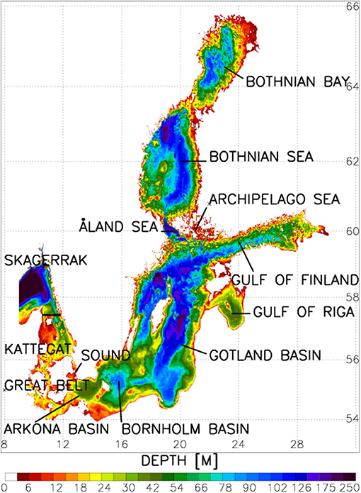
Figure 1. Bottom topography of the Baltic Sea. The Baltic proper comprises the Arkona Basin, Bornholm Basin and Gotland Basin. The solid line marks the border between Kattegat and Skagerrak which is the lateral boundary in BALTSEM and other Baltic Sea models (see text).

To project the future environmental status of the Baltic Sea and to support marine management with nutrient load abatement strategies such as the Baltic Sea Action Plan (BSAP) of the Helsinki Commission (HELCOM) (HELCOM, 2007a,b, 2013a,b), scenario simulations have been developed taking both changing climate and changing anthropogenic nutrient loads into account (e.g., Meier et al., 2011b; Neumann et al., 2012; Omstedt et al., 2012; Saraiva et al., 2018, 2019). For a summary of available future scenario simulations of the biogeochemical cycles of the Baltic Sea, the reader is referred to Table 1.

TABLE 1

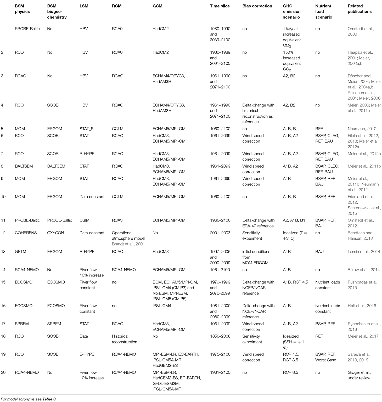
Table 1. Dynamical downscaling experiments for the Baltic Sea for the twenty-first century (BSM, Baltic Sea Model; LSM, Land Surface Model; RCM, Regional Climate Model; GCM, global General Circulation Model; GHG, Greenhouse Gas).

One aim of scenario simulations of the Baltic Sea ecosystem is to provide decision makers with reliable information about multiple stressors (e.g., Jutterström et al., 2014). Hence, dynamical downscaling of global climate change may contribute, in particular, to the development of an improved BSAP in future climate and, in general, to an improved holistic marine management because of the long response time scale of the Baltic Sea of about 30 years (e.g., Omstedt and Hansson, 2006a,b). In this context, the assessment of uncertainties (or knowledge gaps) of scenario simulations is of utmost importance (Mastrandrea et al., 2010).

In general, uncertainties in scenario simulations (here defined as the variances of mean changes between future and historical climates) are caused by climate model uncertainties, by unknown future greenhouse gas (GHG) emissions (or concentrations) and by natural variability (Hawkins and Sutton, 2009). Natural variability has two contributions, i.e. unforced internal and externally driven variations such as solar variability and volcanic eruptions. The latter source of uncertainty is usually neglected, since scenario simulations are not predictions but projections of only anthropogenic climate change (Rummukainen, 2016b). In addition to these three distinct sources inherent to all climate projections, uncertainties in regional projections comprise even the experimental setup of the downscaling approach including for instance lateral boundary conditions such as the global mean sea level rise (Meier et al., 2017) and initial conditions (including the spin up strategy), or unknown regional nutrient load scenarios (Zandersen et al., 2019). Further, insufficient process descriptions in state-of-the-art biogeochemical models for the Baltic Sea such as unknown bioavailable fractions of external nutrient loads (e.g., Eilola et al., 2011), the insufficient description of non-Redfield stoichiometry (e.g., Fransner et al., 2018) and benthic macrofauna (Timmermann et al., 2012), the missing impact of invasive species (e.g., Holopainen et al., 2016; Isaev et al., 2017), the implicit description of the microbial loop (e.g., Wikner and Andersson, 2012), and the lacking top-down cascade in the food web including the impact of fishing (e.g., Niiranen et al., 2013; Nielsen et al., 2017; Bauer et al., 2018, in press) contribute to the overall uncertainties of projections.

In this study, we identify, discuss and rank uncertainties in scenario simulations of the Baltic Sea by assessing the existing literature and by expert judgment. The purpose of the review is to better understand the various sources of uncertainties and to identify knowledge gaps.

In the following two sections, results of scenario simulations of biogeochemical cycles in the Baltic Sea (Background) and the methods used for the projections of coastal seas (Dynamical Downscaling Methods) are reviewed. Further, uncertainties of scenario simulations are qualitatively assessed and their sources are discussed (Results of the Assessment of Uncertainties). Identified or hypothesized uncertainties are related to (1) lack of observations for model calibration, (2–3) differences between projections of General Circulation or Global Climate Models (GCMs) and Regional Climate Models (RCMs), (4) unknown changes in the regional water cycle, (5) natural variability, (6) unknown bioavailable fractions of nutrient loadings from land and the unknown impact of changing climate on nutrient loads, (7) unknown future GHG emission or concentration scenarios, (8) unknown initial conditions of nutrient pools in the water and sediment or unsuitable spin-up simulations due to lack of observations, (9) differences in Global Mean Sea Level (GMSL) projections, (10) lateral boundary conditions, (11) bias correction, (12) differences between projections of the Baltic Sea Models (BSMs), (13) unknown processes of the carbon cycle, and (14) weighting of ensemble members (Table 2). Finally, we discuss methods to estimate and to narrow uncertainties in projections. Weighting is regarded both as a source of uncertainty and as an opportunity to narrow uncertainty. An example illustrating the spread in projected hypoxic area for the Baltic Sea is presented as Supplementary Material. Here, hypoxic area is defined as the area of bottom water with an oxygen concentration less than 2 mL L⁻¹. Conclusions finalize the review. Acronyms used in this study are explained in Table 3.

TABLE 2

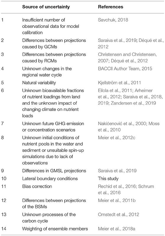
Table 2. Sources of uncertainty addressed by this study and selected key references of the Baltic Sea. For details, the reader is referred to the text.

TABLE 3

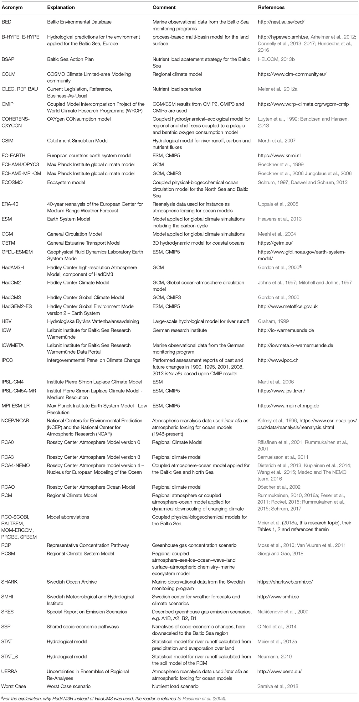
Table 3. List of acronyms, their explanation and references (in alphabetical order).

Background

For the Baltic Sea and North Sea regions detailed assessments of scenario simulations are available (BACC Author Team, 2008; BACCII Author Team, 2015; Schrum et al., 2016; cf. Omstedt, 2017; cf. Räisänen, 2017). Since the first quantitative scenario simulations of biogeochemical cycles in the Baltic Sea did not become available until the year 2010, only the BACCII Author Team (2015) discussed the results of projections of the marine ecosystem published before the year 2012. In the following, we summarize these results of the BACCII Author Team (2015) and of the more recent literature.

Changes in Hydrodynamics

The BACCII Author Team (2015) essentially confirmed the results by the BACC Author Team (2008) concerning water temperature, salinity, sea ice, storm surges and sea level. The projections suggest that the future Baltic Sea would be warmer (between 1.9° and 3.2°C on average) and fresher (between 0.6 and 4.2 g kg⁻¹ on average) than in present climate with a substantial decline in sea-ice cover (between 46 and 77%) and increased storm surges (cf. Meier et al., 2018a). The latter will probably be caused rather by sea-level rise than by increased wind speed (Gräwe et al., 2013). Sea levels are rising primarily as a result of thermal expansion and the loss of land-based ice sheets at global scale (Stocker et al., 2013). Sea levels in the Baltic Sea will follow the global trends but changes will partly be compensated by land-uplift essentially in the northern parts of the Baltic Sea (BACCII Author Team, 2015). Due to the isostatic adjustment after the last glaciation of Fennoscandia, the land is rising with maximum land uplift in the Bothnian Bay close to the Swedish city Luleå of about 0.8 m per century. In the southern Baltic Sea and Kattegat region, land uplift is close to zero.

Newer studies on past and future sea level variability are based on advanced methods and confirm earlier results (e.g., Johansson et al., 2014; Karabil et al., 2017a,b, 2018). Also for sea ice, new projections have been carried out taking the latest results of the Coupled Model Intercomparison Project (CMIP), i.e., CMIP5, into account (e.g., Luomaranta et al., 2014; Seitola et al., 2015). Further, comprehensive work on coastline changes was done (e.g., Harff et al., 2017).

During winter, future runoff may increase in the northern Baltic Sea region whereas in the southern Baltic Sea region the summer runoff will very likely decrease (BACCII Author Team, 2015). The total runoff into the Baltic Sea is projected to increase but figures vary substantially depending on the climate model, GHG emission scenario and downscaling method between about 1 and 21% (Meier et al., 2012c; Donnelly et al., 2014; Saraiva et al., 2019). As most of the variability in salinity is explained by the variability in freshwater supply (Meier and Kauker, 2003a; Schimanke and Meier, 2016), projected salinities are lower than in present climate but the spread among projections is large (Meier et al., 2006). Further, Hordoir et al. (2018) suggested that the estuarine overturning of the Baltic Sea would slow down in warmer climate although the causes are not well understood.

Changes in Biogeochemical Cycles

Changing hydrographic conditions due to changing climate will affect biogeochemical cycles in many ways (e.g., BACCII Author Team, 2015). Higher water temperatures may cause increased algae production and increased remineralization of dead organic material and will reduce the air-sea fluxes of oxygen (Meier et al., 2011b). Furthermore, warming will preferentially favor cyanobacteria blooms compared to the blooms of other phytoplankton species such as diatoms, flagellates and others. The spring bloom is expected to start (and end) earlier (depending on the nutrient and light conditions), and nitrogen fixation might increase (Neumann, 2010; Meier et al., 2012b; Neumann et al., 2012). Indeed, both long-term remote sensing data and BALTSEM (Savchuk, 2002; Gustafsson, 2003; Savchuk et al., 2012a) simulations indicate prolongation of the marine vegetation season in the 2010s comparing to the 1970s, shifting of the annual biomass maximum from spring to summer with the cyanobacteria bloom occurring by half a month earlier, and a tripling of the simulated nitrogen fixation and net primary production (Kahru et al., 2016).

Related to higher air temperatures in future climate is a shrinking sea-ice cover in the northern Baltic Sea that will lead to an earlier onset of the spring bloom due to improved light conditions (Eilola et al., 2013). Due to the reduced sea-ice cover, winds and wave-induced resuspension may increase, causing an increased transport of nutrients from the productive coastal zone into the deeper areas of the northern Baltic Sea. Scenario simulations suggest that increased winter mixing (due to shrinking sea-ice cover) and increased freshwater supply may cause a reduced stratification in the Gulf of Finland (Meier et al., 2011b, 2012a). The reduced sea-ice cover therefore partly counteracts eutrophication because the increased vertical mixing improves oxygen conditions in lower layers.

For the southern Baltic Sea regions without regular seasonal sea-ice cover, it is unclear whether mixing and light conditions will change in future climate because projected changes in wind and cloud cover over the Baltic Sea are uncertain (Räisänen et al., 2004; Kjellström et al., 2011). In a recent study by Gröger et al. (manuscript under review), a consistent northward shift in the mean summer position of the westerly winds was found causing an increase of the wind speed in particular over the southwestern Baltic Sea. For mixing, wind speed extremes are important. However, projected changes in wind speed extremes have a large spread among scenario simulations (Nikulin et al., 2011).

Increasing river runoff together with increased precipitation extremes may reinforce river-borne nutrient loads (Stålnacke et al., 1999; Arheimer et al., 2012; Meier et al., 2012b). However, other drivers than climate change such as sewage treatment and livestock density may become even more important controlling the changes in nutrient loads (e.g., Humborg et al., 2007). Humborg et al. (2007) speculated that riverborne nitrogen loads might increase due to higher livestock densities whereas phosphorus and silica fluxes may decrease due to improved sewage treatment. Such changes would have significant impact on phytoplankton communities. However, these projections do not consider the impact of changing climate on terrestrial biogeochemical processes, which may counteract other anthropogenic effects (Arheimer et al., 2012). Since the 1980, observed phosphorus and nitrogen loads decreased as a response to nutrient load abatement measures (Gustafsson et al., 2012) whereas silicate concentrations showed no significant changes in the northern Baltic proper, Gulf of Finland and Åland Sea during 1979–2011 (Suikkanen et al., 2013). In present climate, silicate is not regarded as limiting nutrient.

As the Baltic Sea is shallow with a mean depth of only 52 m, the nutrient exchange between sediment and water column and resuspension of organic matter are important processes for the biogeochemical cycling. Eilola et al. (2012) suggested that in future climate the exchange between shallow and deeper waters might intensify and that the internal removal of phosphorus might become weaker because of an increased production in the coastal zone and expanding oxygen depletion in the deep water, respectively.

How saltwater inflows may change is unclear (Schimanke et al., 2014). In present climate, no statistically significant trends were found (Mohrholz, 2018). However, global mean sea level rise may enhance the salt transport into the Baltic Sea causing increased stratification, reduced deep water ventilation and expanding hypoxia in the Baltic proper (Meier et al., 2017).

The rising atmospheric CO₂ concentration will lead to a decrease in pH (Omstedt et al., 2012), while eutrophication and enhanced biological production would enhance the seasonal cycle of pH. Eutrophication in the Gulf of Finland is projected to increase assuming a “business-as-usual” (BAU) nutrient load scenario (Lessin et al., 2014). This scenario is characterized by decreasing bottom oxygen concentrations, more frequent anoxic conditions, and increasing phosphate and decreasing nitrate concentrations below 60 m depth. These changes may cause a considerable increase in nitrogen fixation.

In a recent study, a decline in oxygen concentrations in the Bothnian Sea during the last 20 years was found (Ahlgren et al., 2017). This finding is surprising because the Bothnian Sea was so far considered to be oligotrophic. The oxygen depletion was primarily a consequence of warmer water temperature. Further causes were an increase in dissolved organic carbon (DOC) and the import of nutrients from adjacent sub-basins.

Finally, it should be noted that in future climate also the ecosystem structure and functioning is projected to change (BACCII Author Team, 2015). An example is the recent study by Vuorinen et al. (2015), who analyzed the effects of salinity changes on the distribution of marine species. They found a critical shift in the salinity range between 5 and 7 g kg⁻¹, which is a threshold for both freshwater and marine species distributions and diversity. Andersson et al. (2015) provided an overview about future climate change scenarios for the Baltic Sea ecosystem, both for southern and northern sub-basins, and concluded that climate change is likely to have large effects on the marine ecosystem. For instance, in the north heterotrophic bacteria might be favored by allochthonous organic matter, while phytoplankton production may be reduced. In scenario simulations with biogeochemical models, the impact of changing ecosystem structure and function on the biogeochemical cycles are not considered, representing a source of uncertainty.

Changes in Hypoxic Area

Changes in hydrographic conditions and changes in external nutrient loads may cause changes in oxygen depletion and hypoxic area. Meier et al. (2011b) showed with the aid of a multi-model ensemble that hypoxic area might expand in future climate because of increased nutrient loads due to enhanced river runoff, reduced air-sea fluxes and accelerated recycling of organic matter due to higher water temperatures. More frequent and longer lasting periods of hypoxia in future climate (Neumann et al., 2012) may lead to larger phosphorus fluxes from the sediment into the water column (or reduced retention capacity of the sediment) and intensified eutrophication (Meier et al., 2012c; Ryabchenko et al., 2016). Recently, Meier et al. (2018d) found that after saltwater inflows under contemporary environmental conditions oxygen consumption rates in the deep water were accelerated compared to less eutrophied conditions. This acceleration further amplifies deoxygenation in the Baltic Sea and counteract natural ventilation. The reason is that water of inflow events originates mainly from the Baltic surface layer and contains under contemporary environmental conditions, inter alia, higher concentrations of organic matter, zooplankton and higher trophic levels (causing increased heterotrophic oxygen consumption).

Hypoxia is an important indicator of ecosystem health but also a challenge for modeling. In the Supplementary Material, results of past and future changes in hypoxic area of various scenario simulations are summarized.

Dynamical Downscaling Methods

In this section, various dynamical downscaling methods used to perform Baltic Sea projections are reviewed. In general, the dynamical downscaling method uses high-resolution regional simulations to dynamically extrapolate the effects of large-scale climate variability to regional or local scales of interest (Figure 2A). Regional climate atmosphere models have an added value compared to global climate models with respect to the representation of orographic details, the land-sea mask, sea surface boundary conditions (sea surface temperature (SST) and sea ice), more detailed vegetation and soil characteristics, and extremes, e.g., cyclones (e.g., Rummukainen, 2010, 2016a; Feser et al., 2011; Rockel, 2015; Rummukainen et al., 2015). Corresponding arguments apply for regional climate ocean models (e.g., Meier, 2002a). From the ocean perspective, historically the main requests from the regional atmospheric forcing were proper wind fields and atmospheric surface variables that take the changing sea-ice cover in the Baltic Sea under global warming into account (Meier et al., 2011c; their Figure 3). Due to the ice-albedo feedback in the northern Baltic Sea (Bothnian Bay, see Figure 1) winter mean changes in SST and wind speed may differ between individual scenario simulations performed with uncoupled (atmosphere) and coupled (atmosphere–sea-ice–ocean) regional climate models by more than 3°C and 1 m s⁻¹, respectively (Meier et al., 2011c; their Figures 10, 11). Even larger discrepancies were reported from the European PRUDENCE project (Christensen and Christensen, 2007) emphasizing the added value of coupled RCMs. However, the added value of the usage of coupled RCMs or Regional Climate System Models (RCSMs; Giorgi and Gao, 2018) is often overshadowed by the uncertainties from the lateral boundary data from the GCMs or the experimental setup (Schrum, 2017; Mathis et al., 2018).

FIGURE 2

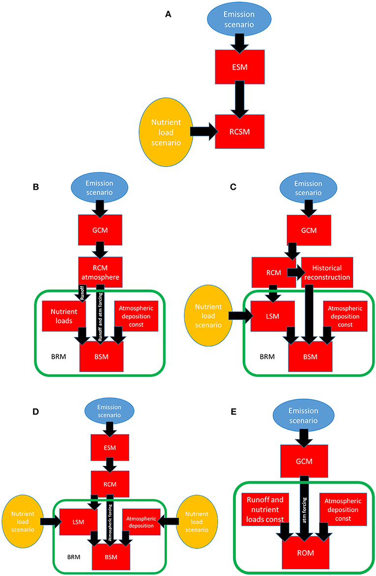
Figure 2. (A) Hierarchy of models in the dynamical downscaling approach (ESM, Earth System Model; RCSM, Regional Climate System Model including atmosphere, sea ice, ocean, land surface and terrestrial vegetation, atmospheric chemistry, marine biogeochemistry, food web, fishery). (B) Hierarchy of models in the dynamical downscaling approach used, e.g., by Neumann (2010) (GCM, General Circulation Model or Global Climate Model; RCM, Regional Climate Model, i.e., a regional atmosphere model; BSM, Baltic Sea Model; BRM, Baltic Region Model including a BSM and data sets for riverine nutrient loads calculated from the product of river runoff and climatological river nutrient concentration and atmospheric deposition). (C) Hierarchy of models in the dynamical downscaling approach used, e.g., by Meier et al. (2011a). Monthly mean changes in atmospheric surface fields were added to a historical reconstruction that forces a Baltic Sea model (LSM, Land Surface Model; BRM, Baltic Region Model including a BSM, LSM, and data sets for atmospheric deposition). (D) Hierarchy of models in the dynamical downscaling approach used, e.g., by Saraiva et al. (2018). (E) Hierarchy of models in the dynamical downscaling approach used, e.g., by Holt et al. (2016) (ROM, Regional Ocean Model for the Black Sea, Barents Sea, North Sea and Baltic Sea, and Northwest European Continental Shelf).

The first scenario simulations of the Baltic Sea based upon coupled physical-biogeochemical ocean circulation models were performed by Neumann (2010) and Meier et al. (2011a). Earlier scenario simulations that have been developed since the end of the 1990s focussed only on hydrodynamic changes in the Baltic Sea (Table 1). Neumann (2010) performed transient simulations for the period 1960–2100 with an ecosystem model driven by the atmospheric and hydrological forcing from a regional climate atmosphere model with sea surface and lateral boundary data from a global climate model, which is in turn driven by two GHG emission scenarios (A1B and B1, see Nakićenović et al., 2000).

Meier et al. (2011a) performed six 30-year time slice experiments driven by two regionalized GCMs, i.e. two control simulations representing present climate (1961–1990) and four simulations with A2 or B2 emission scenario, representing the climate of the late twenty-first century (2071–2100). To regionalize global climate change, the regional coupled atmosphere–sea-ice–ocean model by Döscher et al. (2002) with lateral boundary data from the two GCMs was applied (Räisänen et al., 2004).

Meier et al. (2011a) applied the delta approach for the time slice experiments considering only climatological monthly mean changes of the atmospheric and hydrological forcing together with the reconstructed variability of the period 1969–1998. Hence, they assumed that on interannual and longer time scales the temporal variability of the forcing does not change in future climate.

In recent years, the dynamical downscaling approaches used in these two pioneering studies by Neumann (2010) (Figure 2B) and Meier et al. (2011a) (Figure 2C) were significantly improved (Table 1). For instance, improved versions of GCMs or Earth System Models (ESMs) and RCMs (i.e., coupled atmosphere–sea-ice–ocean models), historical spin up of the BSM, transient simulations (instead of time slices), limited usage of bias correction, expanded multi-model ensembles, more plausible nutrient load scenarios and updated GHG concentration scenarios characterize the latest scenario simulations (e.g., Saraiva et al., 2018, 2019). Since uncertainties are considerable and large ensembles of scenario simulations are needed to estimate uncertainties, the sizes of the ensembles were enlarged with time (e.g., Meier et al., 2011b, 2018a; Omstedt et al., 2012; Holt et al., 2016; Saraiva et al., 2019).

Figure 2 shows various experimental setups of the dynamical downscaling approach. Ideally, boundary data from available GCMs or ESMs would be used to force a RCSM, i.e., a regional coupled atmosphere–sea-ice–land surface–ocean model including the regional carbon and nutrient cycles (Giorgi and Gao, 2018). Hence, changes in atmospheric, hydrological and nutrient forcing of the coastal sea of interest, in this case the Baltic Sea, would be calculated by the RCSM based upon global GHG emission (Nakićenović et al., 2000) or concentration (Moss et al., 2010) scenarios and regional nutrient load scenarios (Zandersen et al., 2019). In case of the ecosystem model comprising even higher trophic levels (e.g., Niiranen et al., 2013; Bauer et al., 2018, in press), also fishery scenarios would be needed (cf. Rose et al., 2010). Regional scenarios of nutrient loads and fishery would be consistently downscaled from global Shared Socio-economic Pathways (SSPs) (Van Vuuren et al., 2011; O'Neill et al., 2014; see Zandersen et al., 2019).

Although the dynamical downscaling approach was improved in recent years, existing methods do not follow the ideal experimental setup described above (Figure 2A) and results still suffer from shortcomings. For instance, the work by Saraiva et al. (2018, 2019) employed a hydrological and biogeochemical Land Surface Model (LSM), E-HYPE (Arheimer et al., 2012; Donnelly et al., 2013), separated from the RCSM (Figure 2D). In a first step, the scenario simulations with a coupled atmosphere–sea-ice–ocean model (RCA4-NEMO, Dieterich et al., 2013; Gröger et al., 2015; Wang et al., 2015; see Table 1) were carried out. Surface fields of precipitation and air temperature over land were stored, bias corrected and used to force the uncoupled E-HYPE model that calculates runoff and nutrient loads into the Baltic Sea (Hundecha et al., 2016). In a second step, the atmospheric forcing from RCA4-NEMO and river runoff and nutrient loads from E-HYPE were used to force the simulations of the coupled physical-biogeochemical model RCO-SCOBI (Meier et al., 2003; Eilola et al., 2009; see Table 1). The reason for the choice of this more complicated and not straightforward approach is that RCA4-NEMO included neither a LSM (just a river routing scheme, see Wang et al., 2015) nor a module for marine biogeochemistry. In addition, the atmospheric deposition of nitrogen was prescribed following the nutrient load scenarios of optimistic conditions (BSAP), reference or “current” conditions (REF) and “worst case” conditions (Worst Case) (Saraiva et al., 2018).

Another approach, that does not follow the ideal experimental setup shown in Figure 2A, omitting even a regional atmosphere climate model was presented by Holt et al. (2016) and Pushpadas et al. (2015) (Figure 2E).

In addition to the models described above, long-records of homogenous observational datasets, e.g., monitoring data, are needed for the development of scenario simulations because climate models have to be calibrated and evaluated for past and present climate variability before they can be used for future projections. In this study, uncertainties related to differing numbers of observations contained in various databases are discussed (Table 4). The insufficient temporal and spatial data coverage may cause errors of integrated data products such as nutrient pools that are used for model calibration and evaluation (Table 5).

TABLE 4

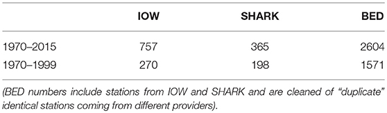
Table 4. Total amount of stations (“station” is a vertical profile sampled; it could be just temperature measured every few centimeters or a full set at standard depths; it could also include multi-day intensive stations with profiles taken every few hours) in different datasets: (1) The data archive (http://iowmeta.io-warnemuende.de) of the Leibniz Institute for Baltic Sea Research Warnemünde (IOW), (2) the Swedish Ocean Archive (SHARK, https://sharkweb.smhi.se/) operated by the Swedish Meteorological and Hydrological Institute (SMHI), and (3) the Baltic Environmental Database (BED, http://nest.su.se/bed) at Stockholm University.

TABLE 5

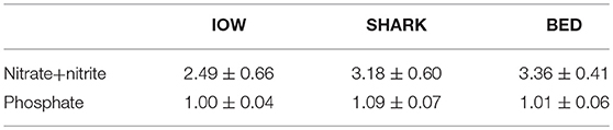
Table 5. Average (2000–2010) basin-wide annual mean concentrations (mmol m⁻³) estimated from different datasets (see Table 4).

Results of the Assessment of Uncertainties

Estimating Uncertainties

Meier et al. (2012c) compared reconstructed past variations and future projections of the Baltic Sea ecosystem and described considerable uncertainties due to model biases, unknown initial conditions, and unknown GHG emission and nutrient load scenarios. Therefore, the significance of scenario simulations is strongly related to the inherent uncertainties. Within the used model chain the assumptions taken, the dynamic behavior of the considered system itself and existing knowledge gaps constitute several sources of uncertainties. They may add up and pollute the simulation results. Finally, conclusions may become weak or are even impossible. However, for marine management combined climate and nutrient load scenario simulations are of utmost importance because of the long time scales of marine biogeochemical cycles. Hence, to be useful in the decision-making process projections have to consider the range of uncertainty. The challenge for research is to discover how a priori assumptions (like unknown future scenarios) affect uncertainty and how uncertainty can be reduced. With this information some management questions can still be answered with the help of scenario simulations despite considerable uncertainties.

Uncertainties of future projections are large, as shown by Meier et al. (2018a). Several differing sources may contribute to these uncertainties (Figure 3, Table 2). Nevertheless, Meier et al. (2018a) showed that in a relatively large ensemble of scenario simulations based on six coupled physical-biogeochemical models of the Baltic Sea the signal-to-noise ratios of temperature and salinity at the surface and in the deep water in Bornholm Basin, Gotland Basin, Gulf of Finland, Bothnian Sea and Bothnian Bay (for the locations see Figure 1) are larger than 1 (Meier et al., 2018a; their Figure 8). Here, the signal-to-noise ratio is defined as the absolute value of the ratio between the ensemble mean change and the standard deviation of the mean changes between future and historical climates calculated from all ensemble members, i.e. the ensemble spread.

FIGURE 3

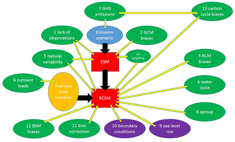
Figure 3. Hierarchy of models in the dynamical downscaling approach as shown by Figure 2 and selected sources of uncertainties as discussed in the text.

However, for biogeochemical variables, such as deep water oxygen concentrations and winter mean surface concentrations of nitrate and phosphate, the signal-to-noise ratios are mostly smaller than 1 suggesting that changes are not significant (Meier et al., 2018a; their Figure 8). Similar results were found by Meier et al. (2012c their Figure 2) using three coupled physical-biogeochemical models of the Baltic Sea.

Uncertainties in scenario simulations have been studied before (e.g., Räisänen, 2001; Hawkins and Sutton, 2009; Rummukainen, 2016b; Ruosteenoja et al., 2016). Hawkins and Sutton (2009) identified three sources of uncertainty in global temperature projections, i.e. model uncertainty, scenario uncertainty and internal variability (see introduction). They applied a statistical formalism based upon average variances of simulated climate change of a smoothed fit of the original time series and variances of the residuals across scenarios and time. They concluded that for lead times of the next few decades or shorter the dominant contributions to the total uncertainty are internal variability and model uncertainty. The importance of internal variability increases at regional compared to global scales and at time scales shorter than a few decades. Consistent with these results, in many studies the statistical significance of simulated climate change between future and past time slices (usually of a 30-year period) was calculated from a Student's t-test (e.g., Räisänen et al., 2004). For longer lead times the dominant sources of uncertainty are model uncertainty and scenario uncertainty according to Hawkins and Sutton (2009). Finally, they concluded that the uncertainties from internal variability and model uncertainty are potentially reducible through better initialization of climate predictions (e.g., Smith et al., 2007; Meehl et al., 2009) and progress in model development although the advantages of improved models are not yet visible (Knutti and Sedláček, 2013).

In a first attempt to quantify uncertainties in scenario simulations of the Baltic Sea, Saraiva et al. (2019) analyzed uncertainties of projected temperature, salinity, primary production, nitrogen fixation and hypoxic area from an ensemble of 21 scenario simulations and two sensitivity experiments using one BSM, one RCM, one hydrological model, four GCMs, two GHG concentration scenarios (i.e., the Representative Concentration Pathways RCP 4.5 and RCP 8.5, see Moss et al., 2010) and three regional nutrient load scenarios ranging from plausible low to high values following Zandersen et al. (2019). Saraiva et al. (2019) analyzed uncertainties at the end of the twenty-first century and consequently neglected the uncertainty from natural variability (Hawkins and Sutton, 2009). Hence, for scenario simulations of the Baltic Sea comprehensive, quantitative analyses of the sources of uncertainty are still not available.

Sources of Uncertainties

Observations

The mechanisms of eutrophication are better explained by total amounts (pools) of nutrients in the aquatic system rather than by concentrations at specific locations because of large horizontal gradients. Therefore, an assessment of uncertainties in the pools reconstructed from observations and used for calibration and validation of the models is very important. The extent of such uncertainties can be demonstrated by a comparison of basin-wide mean concentrations of oxidized nitrogen (NO₃+NO₂) and phosphate for the Baltic proper from different measurement datasets for 2000–2010, the time interval reasonably covered by the national monitoring schemes (Savchuk, 2018). The datasets differ in station distributions and number of observations (Table 4). The comparison suggests that there are systematic differences between the pools reconstructed from the various datasets, larger for oxidized nitrogen than for phosphate (Table 5).

Global Climate Models

Over the Baltic Sea region, 60–70% of the uncertainty in the 4th decade of the projection and still 40–50% in the 9th decade is due to GCM uncertainties (Hawkins and Sutton, 2009; their Figure 6). GCMs and ESMs are usually not tuned to perform well in a specific region but rather to reproduce the dynamics of large-scale key climate processes. Furthermore, the tuning strategy can differ significantly among different modeling groups (e.g., Hourdin et al., 2017; Schmidt et al., 2017) and often the model's climate sensitivity plays a significant role in model calibration (e.g., Mauritsen et al., 2012). Moreover, the long-term development of global models often follows a trend toward more complexity, i.e., inclusion of more processes and more climate components leading to more comprehensive ESMs (see, e.g., the special issue on the development of the MPI-ESM model in Journal of Advances in Modeling Earth Systems¹. However, the advances in global climate modeling will not necessarily translate into a better climate representation on the regional scale. A big problem for the Baltic Sea region still is that it is either not at all spatially resolved or only treated as a lake (e.g., Sein et al., 2015). Thus, even in those GCMs, where the Baltic Sea is included, it does not benefit from the interactive air-sea coupling due to the coarse resolution. Therefore, there is growing evidence that for dynamical downscaling of climate scenarios for the Baltic Sea the use of regional coupled atmosphere-ocean models is beneficial compared to standalone models (e.g., Tian et al., 2013; Gröger et al., 2015).

The number of GCMs that can be downscaled for the region of interest is usually too small to estimate uncertainties. This requires defining criteria for a careful selection of available GCM scenarios. Very recently methods were developed for GCM selection that suggest to select a subset of models that best represents the whole spectrum of available GCMs (e.g., Wilcke and Bärring, 2016). In retrospect, the method by Wilcke and Bärring (2016) motivates the selection of GCMs by Saraiva et al. (2019) who estimated uncertainties in Baltic Sea ecosystem projections due to GCM deficiencies. Saraiva et al. (2019) selected four out of the five GCMs identified by Wilcke and Bärring (2016) to best represent the optimal number of clusters for the spread in projections.

Regional Climate Models

The choice of RCM contributes to the uncertainty of simulated climate in the Baltic Sea first and foremost through the representation of natural variability (Van der Linden and Mitchell, 2009) because biogeochemical cycles in the Baltic Sea are sensitive to atmospheric conditions on shorter time scales, for example, through Major Baltic Inflows (Matthäus and Franck, 1992), storm-induced mixing (Reissmann et al., 2009) or upwelling (Vahtera et al., 2005).

Projections with RCMs inherit the model uncertainty from the GCMs that are used as boundary forcing for the RCMs. In addition, strategies, how the equations are discretized and how sub-grid scale processes are parameterized, contribute to the uncertainties originating from RCMs. Déqué et al. (2007) and Déqué et al. (2012) studied projections of temperature and precipitation over the European region in ensembles of different RCMs driven by different GCMs to determine the contributions of GCM and RCM model uncertainties to the total spread in the projections. They found that in general the GCM has a larger contribution to the spread. This should come as no surprise since RCMs are developed and tuned for a specific region, whereas GCMs need to perform reasonably well everywhere and are mostly tuned to the large open ocean areas. While the choice of the GCM becomes important on seasonal and longer time scales, on shorter time scales the RCM uncertainty dominates. Weekly to hourly time scales are important, for instance, for large salt water inflows, upwelling and mixing.

It has been shown by Deser et al. (2014) that uncertainty on a regional scale can be connected to the natural variability of the system. Different patterns of atmospheric variability like Scandinavian blocking² or a potential shift in the storm track and its effect on the Baltic Sea ecosystem have not been investigated so far. It is conceivable that the choice of the GCM and RCM and even the combination of different GCM/RCM pairs might lead to different representations of these patterns. In order to quantify this added uncertainty, specific experiments need to be carried out for future, more detailed assessments.

Since state-of-the-art multi-model ensembles are using only a selected number of RCMs to drive the Baltic Sea ecosystem models, the uncertainty that stems from the choice of the RCMs is undersampled. Studies like the PRUDENCE project (Christensen and Christensen, 2007) or the CORDEX effort (Jacob et al., 2014) showed that, for example, uncertainties in projections of precipitation are mainly dominated by the RCM in the Baltic Sea drainage basin. One of the most important factors that governs the interaction between the atmosphere and the marine ecosystem is the wind at the atmosphere-ocean interface. The surface wind is also one of those variables that on a regional scale are very much dependent on the choice of the RCM and do affect the solution of the marine ecosystem. On the other hand, integrated measurements like the bottom salinity in the Gotland Basin provide a good test to assess the credibility of a specific RCM and marine ecosystem combination for hindcast periods where reanalyses are available to drive the RCM.

Finally, the choice of the size of the RCM domain is a source of uncertainty. For instance, the freshwater balance of the Mediterranean Sea depends on storm tracks over the North Atlantic, which representation are dependent on the resolution of the models (Gimeno et al., 2012). In addition, atmosphere-ocean feedbacks potentially outside the coupled model domain of the RCM may affect cyclones and heavy precipitation events (Ho-Hagemann et al., 2017).

Regional Water Balance

The global water balance is dominated by precipitation and evaporation at the ocean–atmosphere interface. In coastal seas, such as the Baltic Sea, the land influence is high and on long time scales, the net precipitation over land is balanced by the river runoff to the sea. The precipitation and evaporation rates are strongly influenced by the mid latitudes' low-pressure systems and related trajectories. Fresh water that precipitates over the Baltic Sea catchment area may come from surrounding sea areas such as the Atlantic Ocean, North Sea, Barents Sea or Mediterranean Sea (e.g., Sepp et al., 2018). Long-term changes in the frequency of cyclones and their trajectories are of major importance for the hydrological cycle and for example, the number of cyclones over the Baltic Sea has increased, especially during winter (e.g., Sepp et al., 2005; BACCII Author Team, 2015). During past decades, efforts have been made to analyze the hydrological cycle in the Baltic Basin area by using hydrological models calculating the fresh water drainage to the Baltic Sea (e.g., Graham, 1999). Coastal ocean models were then used to evaluate the water balance calculation (see reviews in Omstedt et al., 2004, 2014) based on available data including salinity measurements. Modeling the Baltic Sea allowed consistent estimates of in- and outflows for closing the hydrological cycles and a possibility to estimate uncertainties with regard to the fresh water cycle in the Baltic Basin area. In the model study by Omstedt and Nohr (2004), all available data were integrated indicating that the long-term net water balances (mean errors over decadal time scales) could be estimated within an error of about ± 600 m³s⁻¹ or 4% of the total river runoff (15,000 m³s⁻¹). By introducing atmospheric and land surface models (e.g., Jacob, 2001; Bengtsson, 2010) it was possible to achieve reasonable estimates of the net fresh water outflow from the Baltic Sea if the atmospheric model was driven by observations based on reanalyzed data at the lateral boundaries. However, estimates on model uncertainties were not analyzed.

Biases and inconsistent climate signals have been reported based on present state-of-the-art RCMs (e.g., Turco et al., 2013). From model calculations on different levels of complexity, the uncertainty in RCMs was estimated using the BALTEX box concept (Raschke et al., 2001). Further, it was shown that especially for climate change impact studies downscaling methods using RCMs still indicate a need for improvement (Omstedt et al., 2000, 2012; Lind and Kjellström, 2009; Donnelly et al., 2014; BACCII Author Team, 2015). For example, Omstedt et al. (2012) showed that without bias corrections related to the fresh water inflow the biogeochemical calculations in the BSMs would be poor. In addition, Donnelly et al. (2014) found that the climate sensitivity of their hydrological model also depends on the bias correction method applied to precipitation and air temperature from the driving RCM.

Natural Variability

The Baltic Sea is affected by internal modes of variability of atmospheric large-scale circulation such as the North Atlantic Oscillation (NAO, e.g., Tinz, 1996; Omstedt and Chen, 2001; Andersson, 2002; Meier and Kauker, 2002; Chen and Omstedt, 2005; Löptien et al., 2013) or decadal and centennial variations related to ocean-atmosphere interactions in the adjacent Atlantic (e.g., Kauker and Meier, 2003; Meier and Kauker, 2003a,b; Hansson and Omstedt, 2008; Schimanke and Meier, 2016; Börgel et al., 2018). Therefore, in order to distinguish natural variations from anthropogenic induced changes, it is crucial to determine the magnitude of natural variability of physical and ecosystem characteristics undisturbed of anthropogenic influence, even though the projected impact of climate change at the end of the century can be expected to be substantially larger than the variability that has been recorded during the historical period.

Previous downscaling studies usually attempted to estimate natural variability from reanalysis data or hindcast simulations by downscaling GCM simulations of the historical period (e.g., Holt et al., 2012; Sein et al., 2015; Wang et al., 2015). In addition, the ensemble approach was applied to distinguish between natural variability and the climate change signal although the number of ensemble members was limited (e.g., three members in Kjellström et al., 2011; Omstedt et al., 2012).

However, anthropogenic influence has already started during the historical period and common hindcast simulations mostly cover the period since 1960. Observation based estimates indicate that the global mean temperature rises at rates between 0.15° and 0.2°C per decade since the seventies of the previous century (e.g., Hansen et al., 2010). Thus, the currently observed warming has already reached about half of the rates which are expected even for the strongest warming projections reported by the assessments of the IPCC, e.g., 0.34°C per decade for the A2 scenario (Meehl et al., 2007) or 0.37°C per decade for the RCP 8.5 scenario (Table 12.2 in Collins et al., 2013). Therefore, estimates of natural variability inferred from any hindcast simulation are already strongly affected by climate warming.

An alternative approach to quantitatively estimate natural variability has been presented by Tinker et al. (2015) and Tinker et al. (2016). They used the regionalized climate from HadCM3 applied to POLCOMS for the northwestern European shelf to downscale 146 years out of a long-term, pre-industrial control simulation from the HadCM3 global climate model. Such a control simulation is unaffected by anthropogenic forcing and thus represents natural variability as realistic as possible. Accordingly, it can even be used to estimate significance of changes simulated during the historical period. The long duration of this simulation likewise allows determining natural variability at low frequencies, which is typically related to the ocean with its higher internal inertia.

An even longer simulation of pre-industrial climate of the Baltic Sea for the period 950-1800 AD was carried out by Schimanke and Meier (2016). These model data allowed to analyze the low-frequency natural climate variability of the Baltic Sea. For instance, Börgel et al. (2018) showed that the Atlantic Multidecadal Oscillation (Knight et al., 2005) has a significant impact on Baltic Sea salinity variations on time scales of 60–90 and 120–180 years for the periods 1450–1650 and 1150–1400, respectively. However, as every GCM generates its own variability characteristics one would have to apply the dynamical downscaling procedure for every individual GCM control climate used in regional multi-GCM ensembles, which makes it computationally quite expensive.

Nutrient Loads and Bioavailability

Although being derived from the same original data (e.g., Savchuk et al., 2012b), different external nutrient inputs were used to calibrate the BSMs, with most important differences originating from the differing assumptions on the bioavailable fractions of land loads taking coastal nutrient retention into account. Especially significant are the differences in terrestrial phosphorus inputs, reaching up to 50% in historical model simulations (Eilola et al., 2011; Meier et al., 2018a; their Figure 3). Recently, Asmala et al. (2017) estimated from up-scaled observations that the coastal filter of the entire Baltic Sea removes 16% of nitrogen (N) and 53% of phosphorus (P) inputs from land, with archipelagos being the most important phosphorus traps. BSMs covering the entire Baltic Sea do not resolve the processes of the coastal zone properly, although shallow areas are included and calibrated to remove “enough” nutrients in the coastal zone to achieve correct nutrient concentrations in the water column of the open sea in present climate. For the entire Swedish coastline, Edman et al. (2018) estimated from a high-resolution coastal zone model the average nutrient filter efficiency to be about 54 and 70% for nitrogen and phosphorus, respectively. As a result, the total amounts and the N:P ratio of nutrients actually entering the open sea biogeochemical cycle are substantially different between the models, which is a source of systematic quantitative differences in scenario responses to projected changes given in absolute amounts.

For instance, in the BALTSEM model the decrease of phosphorus bioavailability from the current 100% would be simply equivalent to a reduction of external input. As had already been shown by Savchuk and Wulff (1999) and was repeatedly confirmed since then, e.g., by hundreds of numerical experiments performed for the revision of the BSAP (Gustafsson and Mörth, 2014), such reduction would result in a weakening of the “vicious circle”³, which is a positive feedback mechanism that impedes the switch from eutrophic to oligotrophic conditions (Vahtera et al., 2007), and would have similar consequences to those already described with the BSAP scenario.

Atmospheric nitrogen depositions amount up to more than 25% of the total loads (HELCOM, 2015). Estimates of atmospheric loads are based on atmospheric transport models calibrated against monitored nitrogen deposition. Modeling relies on emission and land use data. Since not only the HELCOM area contributes to the deposition, also data from outside the HELCOM area and from shipping are used. Past reconstructions may involve larger uncertainties due to missing forcing data and reliable model simulations. Most data have to be considered as rough estimates (Gustafsson et al., 2012).

Some LSMs like HYPE (Arheimer et al., 2012; Donnelly et al., 2013) are process-based and calculate the impact of changing climate on nutrient loads. For instance, Arheimer et al. (2012) suggested that due to the changing climate the total load from the catchment area to the Baltic Sea will decrease for nitrogen and increase for phosphorus in the future. Their scenario simulations indicate that the impact of climate change may be of the same order of magnitude as the expected nitrogen reductions from the measures simulated such as wastewater treatment and agricultural practices. Whereas the knowledge about soil processes on shorter time scales is available, the response to changing climate on longer time scales such as centennial is lacking. Due to sparse observations of long-term trends in the nutrient storage in soil caused by changing climate and land use management, simulated changes in LSMs are difficult to validate.

Emission Scenarios

For addressing uncertainty, new GHG emission scenarios are designed regularly within the framework of CMIP. During phase 3 of CMIP scenarios were defined that provide a range of slower and faster increasing emissions from 2001 onward leading to maximal atmospheric CO₂ concentrations at the end of the twenty-first century (Nakićenović et al., 2000). These scenarios did not include any specific mitigation actions to explicitly reduce emissions but rely more on scenarios for economic growth.

For CMIP5 models, RCPs were developed and define a maximum radiative forcing of GHGs at a certain time with decreasing forcing afterwards. For example, RCP 2.6 has its biggest radiative forcing (~3 W m⁻²) in the middle of the twenty-first century and thereafter it decreases slightly to 2.6 W m⁻² at the end of the century. Thus, when comparing different RCP scenarios, the maximal climate response can be expected at different times depending on the respective RCP. Existing radiative transfer models estimate a present day radiative forcing due to CO₂ of 1.8 W m⁻² and a combined effect of all GHGs of 2.25 W m⁻² (Myhre et al., 1998). More recent estimates of the total radiative forcing from 26 GHGs amount to 2.83 W m⁻² (see Myhre et al., 2013; their Table 8.2, p. 678). It is therefore rather unlikely that RCP 2.6 can be achieved. Hence, this scenario was neglected in most of the previous studies (e.g., Meier et al., 2018a; Saraiva et al., 2018, 2019).

By contrast, the moderate to high radiative forcing scenarios RCP 4.5, RCP 6.0, and RCP 8.5 reach their respective maximum in radiative forcing at the end of the twenty-first century. All RCP scenarios start from the historical period, which ends in 2005. Not considered yet in scenario simulations are the most recent emission scenarios developed in the framework of CMIP6. They are defined from 2015 onward (Eyring et al., 2016) and include a by far more comprehensive suite of possible SSPs compared to the previous phases of CMIP (O'Neill et al., 2014).

The two most commonly used RCP scenarios in Baltic Sea projections, RCP 4.5 and RCP 8.5, are those projections in the CMIP5 program that are included in the core set of experiments (Taylor et al., 2012). In terms of CO₂ emissions, the RCP 8.5 scenario corresponds to the 90th percentile of the scenarios that have been considered for the development of the RCPs (Moss et al., 2010). It represents non-climate policy and high population scenarios. The socio-economic scenario in RCP 8.5 is not unique. Different SSPs would be consistent with this RCP. However, RCP 8.5 may be characterized by fossil fuel dominated economy, high-energy consumption and medium agricultural land use. The RCP 4.5 scenario is a typical mitigation scenario where CO₂ emissions are stabilized after 2080 (Moss et al., 2010). It is compatible with different climate policy scenarios, such as the B1 scenario of the Special Report of Emission Scenarios (SRES) (Nakićenović et al., 2000). It assumes that the population has reached its peak around 2080 at 9 billion people. In the RCP 4.5 scenario, energy consumption is much lower (three fifth) than in RCP 8.5 and coal, oil, gas, bio-energy and nuclear power contribute with roughly equal amounts. Agricultural land use in RCP 4.5 is very low (Van Vuuren et al., 2011).

A noteworthy difference to the currently available RCP scenarios is that the core SSPs, as defined in the CMIP6 ScenarioMIP (Scenario Model Intercomparison Project, O'Neill et al., 2016), include protocols for overshoot scenarios and long-term scenarios that proceed up to 300 years into the future. This refers to the fact that some high impact and non-linear climate responses (e.g., Liu et al., 2017) can occur on time scales beyond the common projection period until 2100. In this long-term perspective, the uncertainty due to the use of different global models is expected to be large, which demands for a high number of ensemble members to be considered in future regional studies.

Initial Conditions

Both, multicomponent ESMs as well as high resolution RCMs have their own internal dynamics and certainly their own individual biases. Therefore, it is highly unlikely that the prescribed initial fields are in phase with internal model dynamics. Especially in the Baltic Sea, which has longer flushing times than many other shelf seas (e.g., the North Sea), this can result in more or less strong model drifts (e.g., Gustafsson et al., 1998; Omstedt et al., 2000; Meier, 2002a). This applies even more to biogeochemical variables involved in carbon and nutrient cycling, and especially to the sediments.

Two approaches have been reported in the literature to overcome this problem: (1) Prolonged spin up runs applying repeated forcing according to present day climate (e.g., Meier, 2007; Lessin et al., 2014), or (2) starting the simulation long before the time period of interest using reconstructed forcing data (e.g., Gustafsson et al., 2012; Meier et al., 2018a,b,c).

The initialization problem becomes more prominent when downscaling GCM climate scenarios. Any initialization from runs other than the corresponding historical run of the global GCM will result in a more or less strong perturbation due to the switch in atmospheric forcing. To remedy this problem, different kinds of bias correction methods have been developed (e.g., Meier, 2006; Meier et al., 2011a; Holt et al., 2012; Mathis et al., 2013; Pushpadas et al., 2015). The general rationale behind those methods is that global GCMs are considered to be sufficiently good to simulate global climate change but are biased on the regional scales (see sub-section on bias correction).

Filtering of nutrients in the coastal zone or burial in the sediments have very long time scales. Hence, the spin up period in many of the state-of-the-art ensemble simulations is too short.

Global Mean Sea Level Rise

Projections of GMSL change range from 0.26 to 0.82 m for the period 2081–2100 relative to 1986–2005 (Stocker et al., 2013). They are dependent on the choice of the emission scenario (Schrum et al., 2016) and natural climate forcing (e.g., solar variability). For the next decades climate variability is already committed by today's GHG levels, whereas long-term projections are more uncertain (Rummukainen, 2016b). A less likely, higher increase in GMSL cannot be ruled out due to possible additional ice sheet contributions (BACCII Author Team, 2015; Schrum et al., 2016).

Uncertainties in GMSL change projections and the different projected spatial patterns arise from the limited capability of the models to simulate climate system processes and natural variability (e.g., El Niño–Southern Oscillation (ENSO) or NAO on regional scales) as the non-linear system of equations has to be solved numerically and is therefore an approximation (Schrum et al., 2016). Horizontal and vertical resolutions are defining the capability of simulating climate system processes and are limited by the available computational resources. In addition, different numerical techniques, parameterizations and model approaches lead to additional uncertainties, which are not well estimated in most studies (Schrum et al., 2016).

Beside the uncertainty of future GMSL change itself, its influence on the Baltic Sea is also uncertain, as only a few studies have investigated this question. Using a process-oriented model Gustafsson (2004) investigated the sensitivity of Baltic Sea salinity to large perturbations in climate such as changes in GMSL and freshwater supply. He found that a rise in GMSL of about + 1 m would lead to a sea surface salinity increase from 8 to 9 g kg⁻¹ in the southern Baltic proper. Hordoir et al. (2015) investigated the influence of GMSL change on saltwater inflows into the Baltic Sea. They performed idealized model sensitivity experiments using a regional ocean general circulation model covering the North Sea and the Baltic Sea. They found that GMSL rise leads to a non-linear increase in salt inflow caused by increased cross-sections and reduced mixing in the Danish straits (Hordoir et al., 2015). However, Arneborg (2016) disproved the interpretation of the results of Hordoir et al. (2015) by arguing that the increased salt inflow caused by GMSL rise is not originating from reduced mixing but is due to a higher increase of barotropic volume fluxes in the Sound than in the Belt Sea.

A study by Meier et al. (2017) investigated the influence of GMSL rise of 0.5 m or 1.0 m on the water exchange between the North Sea and the Baltic Sea and the state of hypoxic areas in the Baltic Sea using a coupled physical-biogeochemical model. Saraiva et al. (2019) even combined scenario simulations with a 1.0 m higher mean sea level. Both studies found a linear increase in salt inflow with increasing cross section and higher stratification in the Baltic Sea and hence increased hypoxic bottom areas. From the performed idealized sensitivity experiments where only time-independent sea level anomalies were added, uncertainties of the scenario simulations by Saraiva et al. (2019) were estimated. However, the simulations overestimate the impact of GMSL rise because they do not take the transient behavior of changing climate into account (Meier et al., 2017).

Uncertainty in Nutrient Concentrations at the Lateral Boundary in the Northern Kattegat/Skagerrak

Regional ocean models usually have a boundary to connecting oceans or seas. Consequently, information at the boundary from outside the model domain is needed. In the case of the Baltic Sea, the effect of the open boundary may be limited due to the bathymetry of the narrow and shallow Danish straits, which confine the exchange between the Baltic Sea and the open ocean. Nevertheless, the effective net import of nitrogen from Kattegat into the Baltic Sea accounts for up to 100 ktons year⁻¹ (Radtke and Maar, 2016)⁴. Here, we will discuss the impact of uncertain information about nutrient concentrations for simulations of the Baltic Sea.

Sources of uncertainty in boundary conditions

According to several earlier estimates, the water masses at the entrance to the Kattegat consist of about 80% of Atlantic waters from the central North Sea, while German Bight and Baltic waters contribute only about 10% each (e.g., Aarup et al., 1996; Kristiansen and Aas, 2015). Despite a marked decrease of nutrient concentrations in the Dutch coastal areas, almost returning to the pre-industrial levels with slightly higher N:P ratio (e.g., Troost et al., 2014; Burson et al., 2016), the concentrations in the offshore areas of the German Bight, where the Jutland Coastal Current originates, have not changed much since the known regime shift in the late 1980s (e.g., Lenhart et al., 2010; Topcu et al., 2011).

A relative stability of the Skagerrak nutrient status has already been demonstrated by Skogen et al. (2004), when drastic reductions of 50% of riverine nutrient input to the North Sea resulted in only about 5% decrease of the simulated primary production in the Skagerrak, which was far less than the natural interannual variations. Less than 15% reduction of primary production has also been simulated with similar nutrient load reductions in several models covering the entire North Sea (Lenhart et al., 2010). Scenario simulations with 50% reductions of the North Sea nitrogen and phosphorus river loads performed with a biogeochemical model for the coupled North Sea - Baltic Sea area resulted in a decrease of the winter surface nitrate and phosphate concentrations at the Skagerrak-Kattegat boundary of 10–20% and 5–10%, respectively (Kuznetsov et al., 2016). The change in nutrient concentrations in the North Sea, Skagerrak and Kattegat due to nutrient load reductions in North Sea rivers is small because of the large exchange of the North Sea water with the Atlantic.

As trends in nutrient concentrations in Atlantic waters filling the southern and central parts of the North Sea have not been observed yet (Radach and Pätsch, 1997; Laane et al., 2005), nutrient concentrations in Skagerrak are usually assumed to be constant. However, as was demonstrated by scenario simulations with a global coupled physical-biogeochemical model with finer resolved northwestern European shelf, the projected warming and freshening sharpens stratification and reduces the upward mixing of nutrient-rich waters along the continental shelf break and their import into the North Sea (Gröger et al., 2013). Consequently, nutrient concentrations in the open North Sea are about halved and primary production is significantly decreased. Recent scenario simulations suggest that the variability in net primary production in the North Sea will rapidly increase after 2080 (Mathis et al., 2019). This non-linear effect is explained by the threshold when the mixed layer depth in the eastern North Atlantic reaches the shelf break causing high-frequent changes in nutrient transports into the North Sea. The impact of such changes for the Baltic Sea has so far not been explored. However, as the nutrient inventory of the Baltic Sea is rather controlled by riverine input and interaction with sediments the effect might probably be small. Efforts to reduce the currently high input of anthropogenic nutrients from, inter alia, fertilizers could give rise to a more prominent role of boundary conditions in the eastern North Sea region in future (see the discussion below).

Impact of uncertainty in boundary conditions

In order to demonstrate the uncertainties introduced into scenario simulations that keep the nutrient inputs from Skagerrak unchanged, BALTSEM simulations have been performed for 300 years under repeated present climate and the contemporary nutrient inputs to the Baltic Sea (HELCOM, 2015) have been kept unchanged except for the inputs through the Skagerrak-Kattegat boundary. Two scenarios have been implemented with reduced boundary nutrient concentrations from the very start of the simulations: “North Sea” (20% nitrogen and 10% phosphorus reduction) and “Atlantic” (50% nitrogen and 50% phosphorus reduction). The comparison of these scenarios to the reference run, where the Skagerrak concentrations are kept unchanged, shows much larger changes in the Kattegat compared to the Gotland Sea, especially in the more plausible “North Sea” scenario (Table 6).

TABLE 6

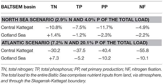
Table 6. Relative changes (in %) of the average (2050–2300) of annual mean nutrient concentrations and integral fluxes induced by the “North Sea” and “Atlantic” scenario reductions of the nitrogen and phosphorus imports from Skagerrak.

The weak response of the Baltic Sea as a whole is explained by the filtering capacity of the shallow and narrow Danish straits. However, in the “Atlantic” scenario the import to the Arkona Basin is reduced by 24 and 28%, i.e., by one half of the relative reductions at the boundary. This small sensitivity might change if the GMSL increases. It is remarkable that even minor reductions of both phosphorus inputs and concentrations lead to a decline of primary production and hypoxic area in the Baltic Sea with a consecutive decrease of denitrification and increase of the phosphorus sediment retention, which in consequence could also be considered as a weakening of the “vicious circle” (Vahtera et al., 2007). Compared to all other uncertainties and overall changes projected by the entire ensemble of available scenario simulations (Meier et al., 2018a), the uncertainties originating from the prescribed nutrient imports from the North Sea can be considered as insignificant. Differences among the models are probably small because the same observations from Kattegat or Skagerrak are used at the lateral boundaries.

Bias Correction

To reduce biases, BSMs and LSMs might be forced by trends calculated from the RCMs/GCMs rather than directly by biased RCM/GCM climates (Rechid et al., 2016; Schrum et al., 2016). However, this method cannot account for biases in wind direction (in earlier studies only wind speed was corrected, e.g., Höglund et al., 2009; Meier et al., 2011c), which may be important in the context of saltwater inflows to the Baltic Sea. Furthermore, atmospheric boundary variables are not independent of each other and their relationships are in most cases non-linear. Hence, the bias corrected forcing variables are in most cases physically not consistent. Further, in case of the Baltic Sea deep water one has to consider that the high sensitivity of inflows to atmospheric forcing (e.g., Schimanke et al., 2014) requires to force and initialize the model with data as close as possible to the forcing data set to which model parameters were originally tuned to. These forcing data are usually various kinds of global (e.g., NCEP/NCAR, Kalnay et al., 1996; ERA-40, Uppala et al., 2005) or regional (e.g., UERRA⁵) atmospheric reanalysis data sets (e.g., Omstedt et al., 2005), gridded observations (e.g., Meier et al., 2003; Omstedt and Hansson, 2006a,b; Meier, 2007), and reconstructions (e.g., Gustafsson et al., 2012; Meier et al., 2012c; Meier et al., 2018b).

On the other hand, bias correction will facilitate the comparison of large ensembles applying multiple driving GCMs (as it removes the individual GCM biases, which must be expected to differ among GCMs) and allows starting the model from conditions as realistic as possible (e.g., Meier et al., 2006; Pushpadas et al., 2015; Holt et al., 2016).

Different Responses/Sensitivity in Baltic Sea Models and Processes

Uncertainties are introduced by both the LSM and the BSM. Since the physical basics of the hydrodynamic modeling are well known, differences in model results emerge merely from the applied numerical approximation of the differential equations and the parameterization of sub-grid scale processes (e.g., Myrberg et al., 2010) or from the atmospheric forcing (Placke et al., 2018). In addition, the model setup like the bathymetry, the open boundary conditions or the treatment of runoff may introduce different model results. Owing to their nature, biogeochemical models are flawed due to the complexity of processes involved and knowledge gaps in their details and parameterizations. The uncertainties in the representation of biogeochemical processes in BSMs were discussed by Eilola et al. (2011). They concluded from the analysis of hindcast simulations of three different BSMs that the largest uncertainties are related to the initial conditions in the early 1960s (the start period of their simulations), the bioavailability of nutrients in land runoff (see section discussion above), the parameterization of sediment fluxes and the turnover of nutrients in the sediments, and the nutrient cycling in the Gulf of Bothnia.

Despite simplification, implemented sediment parameterizations produce biogeochemical fluxes that are reasonably comparable in hindcast simulations to available measurements. However, the integral amounts of sediment nutrients differ between models manifold, which greatly affects the carrying capacity of sediments as ecosystem's memory and makes the response time in projections rather uncertain (Eilola et al., 2011).

Usually in BSMs the response of benthic communities to changing environmental conditions is neglected (e.g., Neumann et al., 2002; Savchuk, 2002; Eilola et al., 2009). Timmermann et al. (2012) showed that benthic fauna has an impact on nutrient sediment fluxes and the feedback between eutrophication and hypoxia. However, Timmermann et al. (2012) concluded that quantitative studies how benthic fauna would affect the system over large spatial and temporal scales are still missing. In particular, the benthic influence on algal blooms and fish populations is quantitatively unknown. Recent simplified simulations of invasive polychaete Marenzelleria spp. in the Gulf of Finland with the SPBEM model demonstrated that the effect would also be similar to a weakening of the “vicious circle” (Isaev et al., 2017).

Models generally strongly underestimate phytoplankton primary production in the Bothnia Bay. For instance, the spring-to-summer reduction of surface nitrate concentration simulated with BALTSEM (8 to 5 μmol L⁻¹) is about a half of the one estimated from measurements (8 to 2 μmol L⁻¹) (Savchuk et al., 2012a). Here, the unknown or poorly parameterized biogeochemical processes might be related to large pools of humic substances, poorer light climate, the relative distribution of bacterial vs. phytoplankton-based production, and the severe phosphorus limitation of the phytoplankton development (Eilola et al., 2011). The assumption on variable phytoplankton stoichiometry instead of the fixed Redfield ratio allowed to somewhat reduce the selected model-data differences (Fransner et al., 2018). However, the implemented parameterizations have yet to be tested in the southern sub-basins of the Baltic Sea. On the other hand, a southward export of nitrogen, underutilized in the Bothnian Bay, is largely assimilated already in the Bothnian Sea.

State-of-the-art models have been developed and evaluated to the present eutrophic situation in the Baltic Sea (Eilola et al., 2011). Evaluation of simulated model results from more oligotrophic pre-industrial times to present (Gustafsson et al., 2012) is therefore important for the assessment of model performance and uncertainties. Historical observations, e.g., of harmful cyanobacteria blooms, are however scarce (Finni et al., 2001) and from pelagic observations we mainly have an understanding about the situation during the eutrophic period in the Baltic Sea. Long records of Secchi depth and oxygen concentrations give some support for historical reconstructions from 1850 forward (Hansson and Gustafsson, 2011; Gustafsson et al., 2012; Meier et al., 2012c, 2018b,c,d; HELCOM, 2013c; Carstensen et al., 2014), but no information about the nutrient cycling or the occurrence of cyanobacteria blooms. Thus, it is difficult to assess the model performance under different forcing conditions like oligotrophic nutrient loads or different climate.

Further, the link to top-down ecosystem pressures and bio-economic scenarios in state-of-the-art BSMs is usually missing. In the recent review by Nielsen et al. (2017), a big number of bio-economic models operating in scenario mode in the Baltic Sea was reviewed. However, these models did not contain a coupled physical-biogeochemical component. Although the approach of end-to-end ecosystem models was already developed many years ago (Fulton, 2010), only a few studies about bottom-up linkages are available for the Baltic Sea (Niiranen et al., 2013; Bauer et al., 2018, in press; Bossier et al., 2018). Usually, state-of-the-art BSMs do not consider higher trophic levels (e.g., Neumann et al., 2002; Savchuk, 2002; Eilola et al., 2009).

Concerning model biases, temperature and salinity dependencies of some key biogeochemical and food web processes are not well understood. For instance, higher temperatures accelerate bacterial mineralization of phosphorus in the bottom sediments, but the overall rate is unknown. Furthermore, Meier et al. (2011b) showed by comparison of scenario simulations with three BSMs, that sensitivities of the ecosystem response to nutrient load changes differ considerably among the models. For instance, they found large differences in bottom oxygen concentration changes. For a given nutrient load scenario the discrepancies are largest in regions along the slopes of the Baltic proper and Gulf of Finland that are affected by the varying position and strength of the halocline. The reasons are runoff and wind speed changes that differ among the climate projections. In addition, the sensitivity of the halocline depth to changes in runoff and wind speed differs among the various BSMs. Further, the sensitivity to changes in nutrient loads (BSAP, REF, and BAU) varies considerably among the models. Despite these uncertainties, all three models agree astonishingly well in their overall response of the ecosystem to changes in the external nutrient supply because the response to nutrient load changes is even larger than the spread of the projections. For instance, Meier et al. (2011b) found that in future climate the BSAP is very likely not as efficient as in present climate and perhaps will not lead to any improvement at all under the prescribed experimental setup. In this respect, all three models agreed.

Carbon Cycle Uncertainties

State-of-the-art marine biogeochemical models are often expanded to include the carbon cycle explicitly (e.g., Omstedt et al., 2009; Edman and Omstedt, 2013; Kuznetsov and Neumann, 2013; Gustafsson et al., 2014a,b).

Measurements of carbonate system parameters in the Baltic Sea cover more than one hundred years. As demonstrated by Müller et al. (2016), total alkalinity (A_T) measurements from 1995 and onwards are particularly consistent (in terms of precision), while measurements, e.g., during the 1965–1995 period, are generally less certain. There are also cases where the handling of sulfidic water samples may have resulted in a considerable underestimation of A_T concentrations (Ulfsbo et al., 2011). These issues have implications for hindcast modeling studies as well as model validation.

Another source of uncertainty is the influence of organic alkalinity. The Baltic Sea is heavily influenced by riverborne loads of organic material. If the alteration of the acid-base balance caused by organic acids is not taken into account in carbonate system calculations, the calculations are unreliable. A bulk dissociation constant and average DOC fraction that contributes to the organic alkalinity have been defined for Baltic Sea waters (Kulinski et al., 2014; Ulfsbo et al., 2015), but spatial differences and temporal changes are as yet not described in detail. Riverine A_T as well as dissolved inorganic carbon concentrations and loads are in addition expected to change in the future as a result of both changes in weathering induced by rising air temperatures, and changes in precipitation patterns (Omstedt et al., 2012).

Omstedt et al. (2015) estimated that the acidification due to the atmospheric deposition of acids peaked around 1980, with a cumulative pH decrease of approximately 0.01 in surface waters and a cumulative reduction of A_T of approximately 30 μmol kg⁻¹. The effect on pH is approximately one order of magnitude less than the cumulative acidification due to increased atmospheric CO₂ concentrations.

The CO₂ exchange between air and sea depends directly on the difference between CO₂ partial pressure (pCO₂) in air and surface water respectively. To reproduce observed pCO₂ by means of model simulations has however proven to be a difficult task. Particularly the main mechanism behind the observed pCO₂ drawdown in surface waters during the productive season has been discussed quite extensively. Processes that could contribute include (1) cold nitrogen fixation by cyanobacteria as well as nutrient replenishment in sunlit layers by migrating plankton organisms (Eggert and Schneider, 2015); (2) efficient utilization of dissolved organic nutrients by phytoplankton (Edman and Anderson, 2014); (3) excessive CO₂ consumption and DOC exudation by phytoplankton, as well as (4) flexible phytoplankton cell stoichiometry (Kreus et al., 2015; Fransner et al., 2018). In addition, the calculated air-sea CO₂ flux is sensitive to the choice of exchange parameterization (Norman et al., 2013; Gustafsson et al., 2015). Fransner et al. (2018) showed for the northern Baltic Sea that beyond non-Redfield stoichiometry an extensive extracellular DOC production contributes to the low observed surface pCO2 during the vegetation period.

In several modeling studies (e.g., Omstedt et al., 2009; Edman and Omstedt, 2013; Gustafsson et al., 2014a) the riverine A_T concentrations were calibrated (based on Hjalmarsson et al. (2008)) so that observed A_T in different sub-basins could be reproduced by the models. These calibrated values are however in many cases considerably higher than the concentrations obtained from measurements (Gustafsson et al., 2014b). This implies either that the quality of measured riverine concentrations is questionable, or that there are other A_T sources in the Baltic Sea that are not accounted for in the model calculations. None of the system-scale physical-biogeochemical BSMs is for example capable of explicitly simulating the coupled phosphorus-iron-sulfur cycling and related A_T production and consumption in sediments. Potentially, A_T generation coupled to anaerobic mineralization processes in sediments (e.g., pyrite burial) could be a significant missing link (Gustafsson et al., 2014b). It is reasonable to assume that this A_T production/consumption depends largely on both sedimentation rate and the expansion of hypoxic and anoxic sediment areas (cf. Reed et al., 2016). Sedimentation rates and hypoxic areas ultimately depend on the magnitude of external nutrient loads, and these loads differ largely in the different future scenarios. The potential impact of changing climate on future A_T concentrations is unknown.

Weighting

Weighting may add another level of uncertainty to the generation of ensemble-based climate projections because the choice and combination of applied metrics is subjective (Christensen et al. (2010). Weigel et al. (2010) discussed the generic risks if weights do not appropriately represent the true underlying uncertainties, e.g., due to large internal variability. However, weighting may also narrow uncertainty by removing outliers as discussed below.

Meier et al. (2018a) analyzed weighted and unweighted changes from an “ensemble of opportunity”, i.e., from an ensemble of uncoordinated experiments from various projects. They found that the skills of the scenario simulations during the historical climate (1980–2005) differ considerably between the models and that the variances of mean changes between historical and future (2072–2097) climates are relatively large depending on the location and variable. Here, skill (or performance of the simulation) is defined as any measure of the agreement between the predictand, i.e., the climate model results during the historical period, and a set of observations, i.e. monitoring data from selected stations of temperature, salinity and phosphate, nitrate, ammonium, oxygen and hydrogen sulfide concentrations. Meier et al. (2018a) evaluated the skills of 29 climate simulations of six BSMs driven by various GCMs and RCMs and by various land surface or hydrological models. The skill was represented in terms of two metrics, the annual or seasonal mean absolute error and the Pearson correlation coefficient measuring the similarity in the shape of mean profiles. As the results of several tested metrics do not differ considerably, Meier et al. (2018a) concluded that weighting may reduce the uncertainties of the projections in the northern Baltic Sea where the discrepancies between weighted and unweighted ensembles are larger and where the skills of the models are lower than in the southern Baltic Sea (Eilola et al., 2011). In the southern Baltic Sea, projections in weighted and unweighted ensembles are rather similar. Hence, Meier et al. (2018a) concluded that the rigorous implementation of the BSAP would result in a significantly improved environmental status in the southern Baltic Sea despite the counteracting impact of changing climate and despite the large uncertainties. However, the relationship between spread and skill is still unknown and deserves further research (Hawkins and Sutton, 2009).

Discussions

In the following, we discuss methods to estimate uncertainty ranges and to reduce uncertainties in projections based on ensemble modeling and weighting of ensemble members.

Estimating Uncertainties

The first attempt by Saraiva et al. (2019) to estimate ranges of uncertainty in projections for the Baltic Sea was based upon the analysis of variances of 30-year mean changes of selected variables between future and historical climates. They found that the response of biogeochemical fluxes, such as primary production and nitrogen fixation, and deep water oxygen conditions, to changing climate depend mainly on the nutrient load scenario. In the case of high nutrient loads (the so-called “fossil-fueled” scenario), the impact of the changing climate on biogeochemical cycles would be considerable whereas in the case of low loads (the BSAP scenario) the impact of changing climate would be negligible (cf. Saraiva et al., 2018). Hence, the dominant source of uncertainty is very likely related to the nutrient load scenario. For primary production, the second largest source of uncertainty was the unknown greenhouse gas concentration scenario and, for nitrogen fixation and hypoxic area, the second largest source originated from the climate model uncertainties, i.e., from model deficiencies affecting inter alia projected stratification changes (Saraiva et al., 2019). Finally, also the large spread in GMSL rise of one meter affected the uncertainties of nitrogen fixation and hypoxic area in agreement with the results by Meier et al. (2017).

In the study by Meier et al. (2018a), the ensemble spread was significantly larger than by Saraiva et al. (2019), as qualitatively illustrated by hypoxic area in the Supplementary Material, because the “ensemble of opportunity” contained both response and scenario uncertainties (Parker, 2013) whereas the ensemble by Saraiva et al. (2019) only partly reflected these uncertainties. According to Parker (2013) response uncertainty is the insufficiently known model sensitivity under a specified scenario and scenario uncertainty refers to the unknown GHG emissions and other external forcings such as nutrient loads. However, in all available ensemble studies of the Baltic Sea the response uncertainty might be underestimated because the models have the same NPZD (Nutrients-Phytoplankton-Zooplankton-Detritus) structure and were not independently developed. Hence, Parker (2013) recommended working more on structural uncertainty, i.e., the uncertainty about the form of the model equations and how they should be solved computationally.

Since Saraiva et al. (2019) underestimated uncertainties in their quantitative assessment by neglecting natural variability and BSM biases, ways forward toward more complete, quantitative assessment of uncertainties would be to apply the method by Hawkins and Sutton (2009) to newly designed, coordinated multi-model ensemble simulations for the Baltic Sea for 1850–2100 (including a suitable spin up). Hawkins and Sutton (2009) defined the internal variability for each model as the variance of the residuals from a smoothed fit of the projection, estimated independently of scenario and lead time. Since the importance of internal variability increases at smaller spatial scales and shorter time scales, it would be interesting to calculate not only the partitioning of uncertainty with time but also the growth of uncertainty from global to regional scales by comparing the variances of GCMs, RCMs, and BSMs.

Potentials to Narrow Uncertainties

As the quality of scenario simulations differs considerably, a strategy might be to reduce the spread in projections (i.e., the uncertainty) by weighting the ensemble members according to their skill during the historical period. The calculated skills might also be used to exclude members with insufficient quality from the ensemble by defining a certain threshold for the applied metric. However, the choice of an appropriate skill metric is subjective as mentioned above. Hence, the calculated weights would depend on the metric and consequently on the specific application. In the northern Baltic Sea, weighting has probably a larger impact on projections of the biogeochemical cycles than in the southern Baltic Sea because of the large impact of the physics. Climate sensitivity depends on feedback mechanisms that differ in different climate states. Hence, skill is at least a necessary (but not a sufficient) condition for the correct climate sensitivity and higher skill reduces uncertainty (Hawkins and Sutton, 2009). Highly sensitive sub-basins are more affected by model deficiencies than other sub-basins. In the northern Baltic Sea, the ice-albedo feedback affects temperature changes, which in turn affect biogeochemical processes (e.g., growth rates, remineralization rates). Further, in present climate the northern sub-basins are weakly stratified. Hence, increased runoff may further reduce the stratification, e.g., in the Gulf of Finland and Bothnian Bay, and consequently enhance the vertical flux of oxygen with the result of improved bottom oxygen concentrations (Meier et al., 2011b). Thus, the large spread in runoff projections causes large uncertainty in oxygen concentrations and biogeochemical cycling because many processes are highly redox-dependent. Due to these feedback mechanisms, weighting may reduce uncertainties by removing outliers. In summary, results of the few available Baltic Sea studies confirm that equally weighted multi-model ensemble means outperform the results of the single ensemble members supporting the multi-model ensemble approach (e.g., Eilola et al., 2011) and that optimal weighting may in principle further reduce the response uncertainty.

Further research on structural uncertainties identified by this review may potentially lead to a reduction of the overall uncertainty in projections. Taking the specific characteristics of the Baltic Sea into account and focusing on the regional scale, the latter might be possible by improving process descriptions in BSMs in particular in the northern Baltic Sea but also elsewhere (see the unknown small-scale processes with impact on the entire system such as sediment-water fluxes and nutrient retention in the sediments under no. 12 and 13, Table 2); by performing sufficiently long model spin ups without switching the atmospheric forcing from historical reconstructions to climate model results during the simulation (no. 8, see Supplementary Material); by improved calculation of bioavailable loads or by accounting for the entire total loads by modeling dissolved organic nutrients as separate variables (Gustafsson et al., 2014a; Vladimirova et al., 2018) (no. 6); by investigating the filter capacity of the coastal zone in the Baltic Sea as in Edman et al. (2018) under different climates (no. 6); by improving the water cycle in RCMs and its response to changing climate (no. 4); and by consideration of GMSL at the lateral boundary of the BSMs (no. 9). As an effort of the scientific community, rigorous statistical and process-based quality controls of models implemented for projections by using available long-term observations (e.g., Eilola et al., 2011; Placke et al., 2018) may lead, extending the discussion on weighting, to a reduction of uncertainties (such as no. 3, 12, 13). For this purpose, more research on the relationship between skill and spread would be needed. Consequently, bias corrections, which are inherent sources of uncertainty in projections (no. 11), are not recommended and should be avoided whenever possible because they may change the models' sensitivity to changes in the forcing.

How Does Uncertainty Affect the Use of Scenarios in Decision-Making and Future Research?

With 43% of the European Union (EU) population living in coastal regions, it is recognized, e.g., in EU Blue Growth strategies that marine areas offer many opportunities for further exploitation to enhance citizens' health, wellbeing and prosperity. However, as these benefits co-exist alongside hazards and risks that may be exacerbated by climate change and other anthropogenic pressures, these opportunities need to be addressed collectively in a science based integrated management approach to ensure a sustainable exploitation of the sea affected by climate change (Jutterström et al., 2014). The way forward is to climate-proof the ongoing implementation of policies, conventions and frameworks for protection of the marine environment, such as HELCOM's BSAP, The Marine Strategy Framework Directive and The Water Framework directives. Hence, projections will be needed even if their uncertainties are considerable. For the implementation of the BSAP, it will have large economic consequences if additional measures are required to reach good environmental status in future climate. Hence, for research it is of utmost importance to quantify uncertainty, to understand the sources of uncertainty and to narrow uncertainty.

How Can We Deal With Uncertainties in Scenario Simulations?

To quantify uncertainty, large multi-model ensembles of scenario simulations are needed. All projections should be presented together with uncertainty ranges. To raise the credibility of models we suggest to perform regular assessments of models and scenario simulations. Regular information about current knowledge on climate change, e.g., presented in publicly available assessments and fact sheets, and a regular dialog on uncertainty between science and policy makers, e.g., within an expert network on climate change, may help to discuss the usage of models and their uncertainties and to weigh the resources spent for mitigation.

Conclusions

We discussed various sources of uncertainties in projections. Although quantitative estimates are lacking, we estimate based on expert judgment of the authors that the biggest uncertainties are caused by (1) unknown current and future bioavailable nutrient loads from land and atmosphere, (2) the experimental setup of the dynamical downscaling (including the spin up strategy), (3) differences between the projections of the GCMs and RCMs, in particular, with respect to GMSL rise and regional water cycle, (4) differing model-specific responses of the simulated biogeochemical cycles to long-term changes in external nutrient loads and climate of the Baltic Sea region, and (5) unknown future greenhouse gas emissions.

Despite considerable uncertainties in scenario simulations of biogeochemical cycles, a list of potentials to narrow uncertainties was identified. As already during the historical period differences between applied bioavailable nutrient loads and the various experimental setups cause large model biases compared to observations, improvements in spin up, atmospheric forcing, bioavailable nutrient load data set, and model calibration may lead to reduced model biases and reduced spread in projections.

We conclude that assessments of scenario simulations and knowledge syntheses such as this review have the potential to narrow uncertainty ranges. Analyses of state-of-the-art multi-model ensemble scenario simulations, thorough assessments of the results and common workshops will result in research proposals for improving models, experimental strategies and weighting procedures to narrow uncertainties.

Data Availability

Observations from the Baltic Environmental Database (BED) are publicly available from http://nest.su.se/bed. Model codes and data used for the analysis of this study are available from the authors upon request.

Author Contributions

Conception and design of the assessment were discussed during two Baltic Earth workshops in Norrköping, Sweden (March 2014) and Warnemünde, Germany (November 2016) in which most of the authors participated. HM developed the idea of the study and coordinated the project. ME and MP helped with preparatory data analysis of model results developed by HM, ME, KE, TN, HA, CD, RF, BG, EG, AI, IK, BM-K, AO, VR, SS and OS. KE, TN, S-EB, CD, CF, MG, BG, EG, IK, AO, VR, and OS wrote sections of the manuscript. MK and MP compiled relevant literature and prepared the reference list. MN helped with the observational data. The final version of the manuscript was edited by OS and HM. All authors contributed to manuscript revision, read and approved the submitted version.

Funding

The research presented in this study is part of the Baltic Earth program (Earth System Science for the Baltic Sea region, see http://www.baltic.earth) and was funded by the BONUS BalticAPP (Well-being from the Baltic Sea–applications combining natural science and economics) project which has received funding from BONUS, the joint Baltic Sea research and development programme (Art 185), funded jointly from the European Union's Seventh Programme for research, technological development and demonstration and from the Swedish Research Council for Environment, Agricultural Sciences and Spatial Planning (FORMAS, grant no. 942-2015-23). Additional support by FORMAS within the project Cyanobacteria life cycles and nitrogen fixation in historical reconstructions and future climate scenarios (1850–2100) of the Baltic Sea (grant no. 214-2013-1449) and by the Stockholm University's Strategic Marine Environmental Research Funds Baltic Ecosystem Adaptive Management (BEAM) is acknowledged. The Baltic Nest Institute is supported by the Swedish Agency for Marine and Water Management through their grant 1:11 - Measures for marine and water environment. AI and VR were funded in the framework of the state assignment of FASO Russia (theme No. 0149-2019-0015).

Conflict of Interest Statement

The authors declare that the research was conducted in the absence of any commercial or financial relationships that could be construed as a potential conflict of interest.

Acknowledgments

The observational data used for the analysis of nutrient content and lateral boundary conditions are open access and were extracted from the Baltic Environmental Database (BED, http://nest.su.se/bed) at Stockholm University and all data providing institutes (listed at http://nest.su.se/bed/ACKNOWLE.shtml) are kindly acknowledged. BED contains observations, inter alia, from the national, long-term environmental monitoring programs such as the Swedish Ocean Archive (SHARK, https://sharkweb.smhi.se/) operated by the Swedish Meteorological and Hydrological Institute (SMHI) or the German Baltic Sea monitoring data archive (http://iowmeta.io-warnemuende.de) operated by the Leibniz Institute for Baltic Sea Research Warnemünde (IOW) (Table 4). Berit Recklebe is acknowledged for editing the reference list. The constructive comments from two reviewers helped to improve the manuscript considerably.

Supplementary Material

The Supplementary Material for this article can be found online at: https://www.frontiersin.org/articles/10.3389/fmars.2019.00046/full#supplementary-material

Footnotes

1. ^available online: https://agupubs.onlinelibrary.wiley.com/doi/toc/10.1002/(ISSN)1942-2466.MPIESM1).

2. ^Scandinavian blocking is a large-scale, persistent atmospheric pattern of high pressure over Scandinavia that redirects migrating cyclones. The range of typical time scales of blocking is several days to even weeks.

3. ^The “vicious circle” is a feedback mechanism that sustains eutrophication in the Baltic Sea and similar systems (Vahtera et al., 2007; Savchuk, 2018). Increased nutrient loads lead to increased algae blooms, mineralization and oxygen consumption in the water column and sediments. Expanding hypoxia increases removal of nitrogen by denitrification, thus decreasing the N:P ratio. Under anoxic conditions, the phosphorus retention capacity of sediments is considerably reduced causing increased phosphorus fluxes from the sediments into the water column. Deficit of nitrogen and increased availability of phosphate enhance nitrogen fixation by cyanobacteria making nitrogen available for other phytoplankton species and thus reinforcing eutrophication.

4. ^The net import from Kattegat amounts to about 11-14 % of the total bioavailable riverborne nitrogen load during 1980-2005 according to Meier et al. (2018a).

5. ^http://www.uerra.eu/

References

Aarup, T., Holt, N., and Højerslev, N. (1996). Optical measurements in the North Sea-Baltic Sea transition zone. II. Water mass classification along the Jutland west coast from salinity and spectral irradiance measurements. Cont. Shelf Res. 16, 1343–1353. doi: 10.1016/0278-4343(95)00076-3

CrossRef Full Text | Google Scholar

Ahlgren, J., Grimvall, A., Omstedt, A., Rolff, C., and Wikner, J. (2017). Temperature, DOC level and basin interactions explain the declining oxygen concentrations in the Bothnian Sea. J. Mar. Syst. 170, 22–30. doi: 10.1016/j.jmarsys.2016.12.010

CrossRef Full Text | Google Scholar

Ahtiainen, H., and Öhman, M. C. (2014). Ecosystem Services in the Baltic Sea: Valuation of Marine and Coastal Ecosystem Services in the Baltic Sea. Vol. 563 of Report TemaNord. Copenhagen: Nordic Council of Ministers. doi: 10.6027/TN2014-563

CrossRef Full Text | Google Scholar

Andersson, A., Meier, H. E. M., Ripzsam, M., Rowe, O., Wikner, J., Haglund, P., et al. (2015). Future climate change scenarios for the Baltic Sea ecosystem and impacts for management. Ambio 44 (Suppl. 3):S345S356. doi: 10.1007/s13280-015-0654-8

CrossRef Full Text | Google Scholar

Andersson, H. C. (2002). Influence of long-term regional and large-scale atmospheric circulation on the Baltic sea level. Tellus A 54, 76–88. doi: 10.3402/tellusa.v54i1.12125

CrossRef Full Text | Google Scholar

Arheimer, B., Dahné, J., and Donnelly, C. (2012). Climate change impact on riverine nutrient load and land-based remedial measures of the Baltic Sea Action Plan. Ambio 41, 600–612. doi: 10.1007/s13280-012-0323-0

PubMed Abstract | CrossRef Full Text | Google Scholar

Arneborg, L. (2016). Comment on “Influence of sea level rise on the dynamics of salt inflows in the Baltic Sea” by R. Hordoir, L. Axell, U. Löptien, H. Dietze, and I. Kuznetsov. J. Geophys. Res. 121, 2035–2040. doi: 10.1002/2015JC011451

CrossRef Full Text | Google Scholar

Asmala, E., Carstensen, J., Conley, D. J., Slomp, C. P., Stadmark, J., and Voss, M. (2017). Efficiency of the coastal filter: nitrogen and phosphorus removal in the Baltic Sea. Limnol. Oceanogr. 62. doi: 10.1002/lno0.10644

CrossRef Full Text | Google Scholar

BACC Author Team (2008). Assessment of Climate Change for the Baltic Sea Basin. Regional Climate Studies. Berlin; Heidelberg: Springer-Verlag. doi: 10.1007/978-3-540-72786-6

CrossRef Full Text

BACCII Author Team (2015). Second assessment of Climate Change for the Baltic Sea Basin. Regional Climate Studies. Springer: Cham. doi: 10.1007/978-3-319-16006-1

CrossRef Full Text

Bauer, B., Gustafsson, B. G., Hyytiäinen, K., Meier, H. E. M., Müller-Karulis, B., and Saraiva, S. (in press). What are potential future states of the Baltic Sea food web? Ambio.

Bauer, B., Meier, H. E. M., Casini, M., Hoff, A., Margonski, P., Orio, A., et al. (2018). Reducing eutrophication increases spatial extent of communities supporting commercial fisheries: a model case study. ICES J. Mar. Sci. 75, 1306–1317. doi: 10.1093/icesjms/fsy023.

CrossRef Full Text | Google Scholar

Bendtsen, J., and Hansen, J. L. (2013). Effects of global warming on hypoxia in the Baltic Sea–North Sea transition zone. Ecol. Model. 264, 17–26. doi: 10.1016/j.ecolmodel.2012.06.018

CrossRef Full Text | Google Scholar

Bengtsson, L. (2010). The global atmospheric water cycle. Environ. Res. Lett. 5:025202. doi: 10.1088/1748-9326/5/2/025202

CrossRef Full Text | Google Scholar

Börgel, F., Frauen, C., Neumann, T., Schimanke, S., and Meier, H. E. M. (2018). Impact of the Atlantic Multidecadal Oscillation on Baltic Sea Variability. Geophys. Res. Lett. 45, 9880–9888. doi: 10.1029/2018GL078943

CrossRef Full Text | Google Scholar

Bossier, S., Palacz, A. P., Nielsen, J. R., Christensen, A., Hoff, A., Maar, M., et al. (2018). The Baltic Sea Atlantis: an integrated end-to-end modelling framework evaluating ecosystem-wide effects of human-induced pressures. PLoS ONE 13:e0199168. doi: 10.1371/journal.pone.0199168

PubMed Abstract | CrossRef Full Text | Google Scholar

Brandt, J., Christensen, J. H., Frohn, J. H., Palmgren, F., Berkowicz, F., and Zlatev, Z. (2001). Operational air pollution forecasts from European to local scale. Atmos. Environ. 35, 91–98. doi: 10.1016/S1352-2310(00)00415-5

CrossRef Full Text | Google Scholar

Bülow, K., Dieterich, C., Elizalde, A., Gröger, M., Heinrich, H., Hüttl-Kabus, S., et al. (2014). Comparison of Three Regional Coupled Ocean Atmosphere Models for the North Sea Under Today's and Future Climate Conditions. KLIWAS Zeitschriftenreihe 27/2014. Koblenz: Bundesanstalt für Gewässerkunde.

Burson, A., Stomp, M., Akil, L., Brussaard, C. P., and Huisman, J. (2016). Unbalanced reduction of nutrient loads has created an offshore gradient from phosphorus to nitrogen limitation in the North Sea. Limnol. Oceanogr. 61, 869–888. doi: 10.1002/lno.10257

CrossRef Full Text | Google Scholar

Carstensen, J., Andersen, J. H., Gustafsson, B. G., and Conley, D. J. (2014). Deoxygenation of the Baltic Sea during the last century. Proc. Natl. Acad. Sci. U.S.A. 111, 5628–5633. doi: 10.1073/pnas.1323156111

PubMed Abstract | CrossRef Full Text | Google Scholar

Chen, D., and Omstedt, A. (2005). Climate-induced variability of sea level in Stockholm: influence of air temperature and atmospheric circulation. Adv. Atmospher. Sci. 22, 655–664. doi: 10.1007/BF02918709

CrossRef Full Text | Google Scholar

Christensen, J. H., and Christensen, O. B. (2007). A summary of the PRUDENCE model projections of changes in European climate by the end of this century. Clim. Change 81, 7–30. doi: 10.1007/s10584-006-9210-7

CrossRef Full Text | Google Scholar

Christensen, J. H., Kjellström, E., Giorgi, F., Lenderink, G., and Rummukainen, M. (2010). Weight assignment in regional climate models. Clim. Res. 44, 179–194. doi: 10.3354/cr00916

CrossRef Full Text | Google Scholar

Collins, M., Knutti, R., Arblaster, J., Dufresne, J.-L., Fichefet, T., Friedlingstein, P., et al. (2013). “Long-term climate change: projections, commitments and irreversibility.” in Climate Change 2013: The Physical Science Basis. IPCC Working Group I Contribution to IPCC AR5, eds T. F. Stocker, D. Quin, G. K. Plattner, M. Tignor, S. K. Allen, J. Boschung, A. Nauels, Y. Xia, V. Bex and P. M. Midgley (Cambridge; New York, NY: Cambridge University Press), 1029–1136.

Google Scholar

Daewel, U., and Schrum, C. (2013). Simulating long-term dynamics of the coupled North Sea and Baltic Sea ecosystem with ECOSMO II: model description and validation. J. Mar. Sys. 119–120, 30–49. doi: 10.1016/j.jmarsys.2013.03.008

CrossRef Full Text | Google Scholar

Déqué, M., Rowell, D., Lüthi, D., Giorgi, F., Christensen, J., Rockel, B., et al. (2007). An intercomparison of regional climate simulations for Europe: assessing uncertainties in model projections. Clim. Change 81, 53–70. doi: 10.1007/s10584-006-9228-x

CrossRef Full Text | Google Scholar

Déqué, M., Somot, S., Sanchez-Gomez, E., Goodess, C., Jacob, D., Lenderink, G., et al. (2012). The spread amongst ENSEMBLES regional scenarios: regional climate models, driving general circulation models and interannual variability. Clim. Dyn. 38, 951–964. doi: 10.1007/s00382-011-1053-x

CrossRef Full Text | Google Scholar

Deser, C., Phillips, A. S., Alexander, M. A., and Smoliak, B. V. (2014). Projecting North American climate over the next 50 years: uncertainty due to internal variability. J. Clim. 27, 2271–2296. doi: 10.1175/JCLI-D-13-00451.1

CrossRef Full Text | Google Scholar

Dieterich, C., Schimanke, S., Wang, S., Väli, G., Liu, Y., Hordoir, R., et al. (2013). Evaluation of the SMHI Coupled Atmosphere-Ice-Ocean Model RCA4-NEMO, Vol. 47 of Report Oceanography. Norrköping: SMHI.

Google Scholar

Donnelly, C., Arheimer, B., Capell, R., Dahn,é, J., and Strömqvist, J. (2013). “Regional overview of nutrient load in Europe – challenges when using a large-scale model approach, E-HYPE,” in Proceedings of H04, IAHS-IAPSO-IASPEI Assembly, Vol. 361 (Gothenburg: IHS Publication), 49–58.

Donnelly, C., Greuell, W., Andersson, J., Gerten, D., Pisacane, G., Roudier, P., et al. (2017). Impacts of climate change on European hydrology at 1.5, 2 and 3 degrees mean global warming above preindustrial level. Clim. Change 143, 13–26. doi: 10.1007/s10584-017-1971-7

CrossRef Full Text | Google Scholar

Donnelly, C., Yang, W., and Dahn,é, J. (2014). River discharge to the Baltic Sea in a future climate. Clim. Change 122, 157–170. doi: 10.1007/s10584-013-0941-y

CrossRef Full Text | Google Scholar

Döscher, R., and Meier, H. E. M. (2004). Simulated sea surface temperature and heat fluxes in different climates of the Baltic Sea. Ambio 33, 242–248. doi: 10.1579/0044-7447-33.4.242

PubMed Abstract | CrossRef Full Text | Google Scholar

Döscher, R., Willén, U., Jones, C., Rutgersson, A., Meier, H. E. M., Hansson, U., et al. (2002). The development of the regional coupled ocean-atmosphere model RCAO. Boreal Environ. Res. 7, 183–192.

Edman, M., Eilola, K., Almroth-Rosell, E., Meier, H. E. M., Wåhlström, I., and Arneborg, L. (2018). Nutrient retention along the Swedish coastline. Front. Mar. Sci. 5:415. doi: 10.3389/fmars.2018.00415

CrossRef Full Text | Google Scholar

Edman, M., and Omstedt, A. (2013). Modeling the dissolved CO₂ system in the redox environment of the Baltic Sea. Limnol. Oceanogr. 58, 74–92. doi: 10.4319/lo.2013.58.1.0074

CrossRef Full Text | Google Scholar

Edman, M. K., and Anderson, L. G. (2014). Effect on pCO₂ by phytoplankton uptake of dissolved organic nutrients in the Central and Northern Baltic Sea, a model study. J. Mar. Syst. 139, 166–182. doi: 10.1016/j.jmarsys.2014.06.004

CrossRef Full Text | Google Scholar

Eggert, A., and Schneider, B. (2015). A nitrogen source in spring in the surface mixed-layer of the Baltic Sea: evidence from total nitrogen and total phosphorus data. J. Mar. Syst. 148, 39–47. doi: 10.1016/j.jmarsys.2015.01.005

CrossRef Full Text | Google Scholar

Eilola, K., Almroth-Rosell, E., Dieterich, C., Fransner, F., Höglund, A., and Meier, H. E. M. (2012). Modeling nutrient transports and exchanges of nutrients between shallow regions and the open Baltic Sea in present and future climate. Ambio 41, 586–599. doi: 10.1007/s13280-012-0317-y

PubMed Abstract | CrossRef Full Text | Google Scholar

Eilola, K., Gustafsson, B. G., Kuznetsov, I., Meier, H. E. M., Neumann, T., and Savchuk, O. P. (2011). Evaluation of biogeochemical cycles in an ensemble of three state-of-the-art numerical models of the Baltic Sea. J. Mar. Syst. 88, 267–284. doi: 10.1016/j.jmarsys.2011.05.004

CrossRef Full Text | Google Scholar

Eilola, K., Mårtensson, S., and Meier, H. E. M. (2013). Modeling the impact of reduced sea ice cover in future climate on the Baltic Sea biogeochemistry. Geophys. Res. Lett. 40, 149–154. doi: 10.1029/2012GL054375

CrossRef Full Text | Google Scholar

Eilola, K., Meier, H. E. M., and Almroth, E. (2009). On the dynamics of oxygen, phosphorus and cyanobacteria in the Baltic Sea; A model study. J. Mar. Syst. 75, 163–184. doi: 10.1016/j.jmarsys.2008.08.009

CrossRef Full Text | Google Scholar

Eyring, V., Bony, S., Meehl, G. A., Senior, C. A., Stevens, B., Stouffer, R. J., et al. (2016). Overview of the Coupled Model Intercomparison Project Phase 6 (CMIP6) experimental design and organization. Geosci. Model Dev. 9, 1937–1958. doi: 10.5194/gmd-9-1937-2016

CrossRef Full Text | Google Scholar

Feser, F., Rockel, B., von Storch, H., Winterfeldt, J., and Zahn, M. (2011). Regional climate models add value to global model data: a review and selected examples. Bull. Am. Meteorol. Soc. 92, 1181–1192. doi: 10.1175/2011BAMS3061.1

CrossRef Full Text | Google Scholar

Finni, T., Kononen, K., Olsonen, R., and Wallström, K. (2001). The history of cyanobacterial blooms in the Baltic Sea. Ambio 30, 172–178. doi: 10.1579/0044-7447-30.4.172

PubMed Abstract | CrossRef Full Text | Google Scholar

Fransner, F., Gustafsson, E., Tedesco, L., Vichi, M., Hordoir, R., Roquet, F., et al. (2018). Non-Redfieldian dynamics explain seasonal pCO₂ drawdown in the Gulf of Bothnia. J. Geophys. Res. Oceans 123, 166–188. doi: 10.1002/2017JC013019

CrossRef Full Text | Google Scholar

Friedland, R., Neumann, T., and Schernewski, G. (2012). Climate change and the Baltic Sea action plan: model simulations on the future of the western Baltic Sea. J. Mar. Syst. 105, 175–186. doi: 10.1016/j.jmarsys.2012.08.002

CrossRef Full Text | Google Scholar

Fulton, E. A. (2010). Approaches to end-to-end ecosystem models. J. Mar. Syst. 81, 171–183. doi: 10.1016/j.jmarsys.2009.12.012

CrossRef Full Text | Google Scholar

Gimeno, L., Stohl, A., Trigo, R. M., Dominguez, F., Yoshimura, K., Yu, L., et al. (2012). Oceanic and terrestrial sources of continental precipitation. Rev. Geophys. 50:RG4003. doi: 10.1029/2012RG000389

CrossRef Full Text | Google Scholar

Giorgi, F., and Gao, X.-J. (2018). Regional earth system modeling: review and future directions. Atmos. Oceanic Sci. Lett. 11, 189–197. doi: 10.1080/16742834.2018.1452520

CrossRef Full Text | Google Scholar

Gordon, C., Cooper, C., Senior, C. A., Banks, H., Gregory, J. M., Johns, T. C., et al. (2000). The simulation of SST, sea ice extents and ocean heat transports in a version of the Hadley Centre coupled model without flux adjustments. Clim. Dyn. 16, 147–168. doi: 10.1007/s003820050010

CrossRef Full Text | Google Scholar

Graham, P. (1999). Modeling runoff to the Baltic Sea. Ambio 28, 328–334.

Google Scholar

Gräwe, U., Friedland, R., and Burchard, H. (2013). The future of the western Baltic Sea: two possible scenarios. Ocean Dyn. 63, 901–921. doi: 10.1007/s10236-013-0634-0

CrossRef Full Text | Google Scholar

Gröger, M., Dieterich, C., Meier, H. E. M., and Schimanke, S. (2015). Thermal air–sea coupling in hindcast simulations for the North Sea and Baltic Sea on the NW European shelf. Tellus A 67:26911. doi: 10.3402/tellusa.v67.26911

CrossRef Full Text | Google Scholar

Gröger, M., Maier-Reimer, E., Mikolajewicz, U., Moll, A., and Sein, D. (2013). NW European shelf under climate warming: implications for open ocean-shelf exchange, primary production, and carbon absorption. Biogeosciences 10, 3767–3792. doi: 10.5194/bg-10-3767-2013

CrossRef Full Text | Google Scholar

Gustafsson, B. G. (2003). A Time-Dependent Coupled-Basin Model for the Baltic Sea. Report C47, Earth Sciences Centre, Göteborg University, Göteborg.

Gustafsson, B. G. (2004). Sensitivity of Baltic Sea salinity to large perturbations in climate. Clim. Res. 27, 237–251. doi: 10.3354/cr027237

CrossRef Full Text | Google Scholar

Gustafsson, B. G., and Mörth, C. M. (2014). Revision of the Maximum Allowable Inputs and Country Allocation Scheme of the Baltic Sea Action Plan. Baltic Nest Institute, Stockholm University.

Gustafsson, B. G., Schenk, F., Blenckner, T., Eilola, K., Meier, H. E. M., Müller-Karulis, B., et al. (2012). Reconstructing the development of Baltic Sea eutrophication 1850–2006. Ambio 41, 534–548. doi: 10.1007/s13280-012-0318-x

PubMed Abstract | CrossRef Full Text | Google Scholar

Gustafsson, E., Deutsch, B., Gustafsson, B. G., Humborg, C., and Mörth, C.-M. (2014a). Carbon cycling in the Baltic Sea - The fate of allochthonous organic carbon and its impact on air-sea CO₂ exchange. J. Mar. Syst. 129, 289–302. doi: 10.1016/j.jmarsys.2013.07.005

CrossRef Full Text | Google Scholar

Gustafsson, E., Omstedt, A., and Gustafsson, B. G. (2015). The air-water CO₂ exchange of a coastal sea - A sensitivity study on factors that influence the absorption and outgassing of CO₂ in the Baltic Sea. J. Geophys. Res. 120, 5342–5357. doi: 10.1002/2015JC010832

CrossRef Full Text | Google Scholar

Gustafsson, E., Wällstedt, T., Humborg, C., Mörth, C.-M., and Gustafsson, B. G. (2014b). External total alkalinity loads versus internal generation: the influence of nonriverine alkalinity sources in the Baltic Sea. Global Biogeochem. Cycles 28, 1358–1370. doi: 10.1002/2014GB004888

CrossRef Full Text | Google Scholar

Gustafsson, N., Nyberg, L., and Omstedt, A. (1998). Coupling of a high-resolution atmospheric model and an ocean model for the Baltic Sea. Month. Weather Rev. 126, 2822–2846. doi: 10.1175/1520-0493(1998)126<2822:COAHRA>2.0.CO;2

CrossRef Full Text | Google Scholar

Haapala, J., Meier, H. E. M., and Rinne, J. (2001). Numerical investigations of future ice conditions in the Baltic Sea. Ambio 30, 237–244. doi: 10.1579/0044-7447-30.4.237

PubMed Abstract | CrossRef Full Text | Google Scholar

Hansen, J., Ruedy, R., Sato, M., and Lo, K. (2010). Global surface temperature change. Rev. Geophys. 48:RG4004. doi: 10.1029/2010RG000345

CrossRef Full Text | Google Scholar

Hansson, D., and Gustafsson, E. (2011). Salinity and hypoxia in the Baltic Sea since A.D. 1500. J. Geophys. Res. 116:C03027. doi: 10.1029/2010JC006676

CrossRef Full Text | Google Scholar

Hansson, D., and Omstedt, A. (2008). Modelling the Baltic Sea ocean climate on centennial time scale: temperature and sea ice. Clim. Dyn. 30, 763–778. doi: 10.1007/s00382-007-0321-2

CrossRef Full Text | Google Scholar

Harff, J., Furmanczyk, K., and von Storch, H. (2017). Coastline Changes of the Baltic Sea from South to East: Past and Future Projection. Cham: Springer International Publishing. doi: 10.1007/978-3-319-49894-2

CrossRef Full Text | Google Scholar

Hawkins, E., and Sutton, R. (2009). The potential to narrow uncertainty in regional climate predictions. Bull. Am. Meteorol. Soc. 90, 1095–1108. doi: 10.1175/2009BAMS2607.1

CrossRef Full Text | Google Scholar

Heavens, N. G., Ward, D. S., and Natalie, M. M. (2013). Studying and projecting climate change with earth system models. Nat. Educ. Knowl. 4:4.

HELCOM (2007a). “Baltic Sea action plan,” in HELCOM Ministerial Meeting 2007 (Krakow).

HELCOM (2007b). “Towards a Baltic Sea unaffected by Eutrophication. HELCOM overview 2007,” in Background Document for the HELCOM Ministerial Meeting (Helsinki).

HELCOM (2013a). “Approaches and methods for eutrophication target setting in the Baltic Sea region,” in Baltic Sea Environment Proceedings, Vol. 133. (Helsinki).

HELCOM (2013b). Copenhagen Ministerial Declaration, HELCOM Ministerial Meeting (Copenhagen).

HELCOM (2013c). “Summary report on the development of revised Maximum Allowable Inputs (MAI) and updated Country Allocated Reduction Targets (CART) of the Baltic Sea Action Plan,” in Background Document for the 2013 HELCOM Ministerial Meeting (Helsinki).

HELCOM (2015). “Updated Fifth Baltic Sea pollution load compilation (PLC-5.5),” in Baltic Sea Environment Proceedings No. 145 (Helsinki).

HELCOM (2018a). “Sources and pathways of nutrients to the Baltic Sea,” in Baltic Sea Environment Proceedings No. 153 (Helsinki).

HELCOM (2018b). “Inputs of Nutrients to the Subbasins,” in HELCOM Core Indicator Report. Available online at: http://www.helcom.fi/baltic-sea-trends/indicators/inputs-of-nutrients-to-the-subbasins (Accessed Dec 5, 2018).

Hjalmarsson, S., Wesslander, K., Anderson, L. G., Omstedt, A., Perttila, M., and Mintrop, L. (2008). Distribution, long-term development and mass balance calculation of total alkalinity in the Baltic Sea. Cont. Shelf Res. 28, 593–601. doi: 10.1016/j.csr.2007.11.010

CrossRef Full Text | Google Scholar

Höglund, A., Meier, H. E. M., Broman, B., and Kriezi, E. (2009). Validation and Correction of Regionalised ERA-40 Wind Fields Over the Baltic Sea Using the Rossby Centre Atmosphere model RCA3.0, Rapport Oceanografi 97. SMHI: Norrköping.

Google Scholar

Ho-Hagemann, H. T. M., Gröger, M., Rockel, B., Geyer, B., Zahn, M., and Meier, H. E. M. (2017). Effects of air-sea coupling over the North Sea and the Baltic Sea on simulated summer precipitation over Central Europe. Clim. Dyn. 49, 3851–3876. doi: 10.1007/s00382-017-3546-8

CrossRef Full Text | Google Scholar

Holopainen, R., Lehtiniemi, M., Meier, H. E. M., Albertsson, J., Gorokhova, E., Kotta, J., et al. (2016). Impacts of changing climate on the non-indigenous invertebrates in the northern Baltic Sea by end of the 21st century. Biol. Invasions 18, 3015–3032. doi: 10.1007/s10530-016-1197-z

CrossRef Full Text | Google Scholar

Holt, J., Butenschoen, M., Wakelin, S. L., Artioli, Y., and Allen, J. I. (2012). Oceanic controls on the primary production of the northwest European continental shelf: model experiments under recent past conditions and a potential future scenario. Biogeosciences 9, 97–117. doi: 10.5194/bg-9-97-2012

CrossRef Full Text | Google Scholar

Holt, J., Schrum, C., Cannaby, H., Daewel, U., Allen, I., Artioli, Y., et al. (2016). Potential impacts of climate change on the primary production of regional seas: a comparative analysis of five European seas. Prog. Oceanogr. 140, 91–115. doi: 10.1016/j.pocean.2015.11.004.

CrossRef Full Text | Google Scholar

Hong, B., Swaney, D. P., Mörth, C.-M., Smedberg, E., Hägg, H. E., Humborg, C., et al. (2012). Evaluating regional variation of net anthropogenic nitrogen and phosphorus inputs (NANI/NAPI), major drivers, nutrient retention pattern and management implications in the multinational areas of Baltic Sea basin. Ecol. Model. 227, 117–135. doi: 10.1016/j.ecolmodel.2011.12.002

CrossRef Full Text | Google Scholar

Hordoir, R., Axell, L., Löptien, U., Dietze, H., and Kuznetsov, I. (2015). Influence of sea level rise on the dynamics of salt inflows in the Baltic Sea. J. Geophys. Res. Oceans 120, 6653–6668. doi: 10.1002/2014JC010642

CrossRef Full Text | Google Scholar

Hordoir, R., Höglund, A., Pemberton, P., and Schimanke, S. (2018). Sensitivity of the overturning circulation of the Baltic Sea to climate change, a numerical experiment. Clim. Dyn. 50, 1425–1437. doi: 10.1007/s00382-017-3695-9

CrossRef Full Text | Google Scholar

Hourdin, F., Mauritsen, T., Gettelman, A., Golaz, J.-C., Balaji, V., Duan, Q., et al. (2017). The art and science of climate model tuning. Bull. Am. Meteorol. Soc. 98, 589–602. doi: 10.1175/BAMS-D-15-00135.1

CrossRef Full Text | Google Scholar

Humborg, C., Mörth, C.-M., Sundbom, M., and Wulff, F. (2007). Riverine transport of biogenic elements to the Baltic Sea – past and possible future perspectives. Hydrol. Earth Syst. Sci. 11, 1593–1607. doi: 10.5194/hess-11-1593-2007

CrossRef Full Text | Google Scholar

Hundecha, Y., Arheimer, B., Donnelly, C., and Pechlivanidis, I. (2016). A regional parameter estimation scheme for a pan-European multi-basin model. J. Hydrol. Reg. Stud. 6, 90–111. doi: 10.1016/j.ejrh.2016.04.002

CrossRef Full Text | Google Scholar

Isaev, A. V., Eremina, T. R., Ryabchenko, V. A., and Savchuk, O. P. (2017). Model estimates of the impact of bioirrigation activity of Marenzelleria spp. on the Gulf of Finland ecosystem in a changing climate. J. Mar. Syst. 171, 81–88. doi: 10.1016/j.jmarsys.2016.08.005

CrossRef Full Text | Google Scholar

Jacob, D. (2001). A note to the simulation of the annual and inter-annual variability of the water budget over the Baltic Sea drainage basin. Meteorol. atmosphere. Phys. 77, 61–73. doi: 10.1007/s007030170017

CrossRef Full Text | Google Scholar

Jacob, D., Petersen, J., Eggert, B., Alias, A., Christensen, O. B., Bouwer, L. M., et al. (2014). EURO-CORDEX: new high-resolution climate change projections for European impact research. Reg. Environ. Change 14, 563–578. doi: 10.1007/s10113-013-0499-2

CrossRef Full Text | Google Scholar

Johansson, M. M., Pellikka, H., Kahma, K. K., and Ruosteenoja, K. (2014). Global sea level rise scenarios adapted to the Finnish coast. J. Mar. Syst. 129, 35–46. doi: 10.1016/j.jmarsys.2012.08.007

CrossRef Full Text | Google Scholar

Johns, T. C., Carnell, R. E., Crossley, J. F., Gregory, J. M., Mitchell, J. F. B., Senior, C. A., et al. (1997). The second Hadley Centre coupled ocean-atmosphere GCM: model description, spinup and validation. Clim. Dyn. 13, 103–134. doi: 10.1007/s003820050155

CrossRef Full Text | Google Scholar

Jungclaus, J. H., Botzet, M., Haak, H., Keenlyside, N., Luo, J.-J., Latif, M., et al. (2006). Ocean circulation and tropical variability in the coupled ECHAM5/MPI-OM. J. Clim. 19, 3952–3972. doi: 10.1175/JCLI3827.1

CrossRef Full Text | Google Scholar

Jutterström, S., Andersson, H., Omstedt, A., and Malmaeus, J. (2014). Multiple stressors threatening the future of the Baltic Sea - Kattegat marine ecosystem: implications for policy and management actions. Mar. Pollut. Bull. 86, 468–480. doi: 10.1016/j.marpolbul.2014.06.027

PubMed Abstract | CrossRef Full Text | Google Scholar

Kahru, M., Elmgren, R., and Savchuk, O. P. (2016). Changing seasonality of the Baltic Sea. Biogeosciences 13, 1009–1018. doi: 10.5194/bg-13-1009-2016

CrossRef Full Text | Google Scholar

Kalnay, E., Kanamitsu, M., Kistler, R., Collins, W., Deaven, D., Gandin, L., et al. (1996). The NCEP/NCAR 40-year reanalysis project. Bull. Am. Meteorol. Soc. 77, 437–471. doi: 10.1175/1520-0477(1996)077<0437:TNYRP>2.0.CO;2

CrossRef Full Text | Google Scholar

Karabil, S., Zorita, E., and Baehr, J. (2017a). Mechanisms of variability in decadal sea-level trends in the Baltic Sea over the 20th century. Earth Syst. Dyn. 8, 1031–1046. doi: 10.5194/esd-8-1031-2017

CrossRef Full Text | Google Scholar

Karabil, S., Zorita, E., and Baehr, J. (2017b). Mechanisms of Sea Level Variability in the Baltic Sea Region for the Period 1850-2100. Doctoral dissertation, Universität Hamburg, Hamburg.

Google Scholar

Karabil, S., Zorita, E., and Hünicke, B. (2018). Contribution of atmospheric circulation to recent off-shore sea-level variations in the Baltic Sea and the North Sea. Earth Syst. Dyn. 9, 69–90. doi: 10.5194/esd-9-69-2018

CrossRef Full Text | Google Scholar

Kauker, F., and Meier, H. E. M. (2003). Modeling decadal variability of the Baltic Sea: 1. Reconstructingatmospheric surface data for the period 1902-1998. J. Geophys. Res. Oceans 108:3267. doi: 10.1029/2003JC001797

CrossRef Full Text | Google Scholar

Kjellström, E., Nikulin, G., Hansson, U. L. F., Strandberg, G., and Ullerstig, A. (2011). 21st century changes in the European climate: uncertainties derived from an ensemble of regional climate model simulations. Tellus A 63, 24–40. doi: 10.1111/j.1600-0870.2010.00475.x

CrossRef Full Text | Google Scholar

Knight, J. R., Allan, R. J., Folland, C. K., Vellinga, M., and Mann, M. E. (2005). A signature of persistent natural thermohaline circulation cycles in observed climate. Geophys. Res. Lett. 32:L20708. doi: 10.1029/2005GL024233

CrossRef Full Text | Google Scholar

Knutti, R., and Sedláček, J. (2013). Robustness and uncertainties in the new CMIP5 climate model projections. Nat. Clim. Chang. 3:369. doi: 10.1038/nclimate1716

CrossRef Full Text | Google Scholar

Kreus, M., Schartau, M., Engel, A., Nausch, M., and Voss, M. (2015). Variations in the elemental ratio of organic matter in the central Baltic Sea: Part I-Linking primary production to remineralization. Cont. Shelf Res. 100, 25–45. doi: 10.1016/j.csr.2014.06.015

CrossRef Full Text | Google Scholar

Kristiansen, T., and Aas, E. (2015). Water type quantification in the Skagerrak, the Kattegat and off the Jutland west coast. Oceanologia 57, 177–195. doi: 10.1016/j.oceano.2014.11.002

CrossRef Full Text | Google Scholar

Kulinski, K., Schneider, B., Hammer, K., Machulik, U., and Schulz-Bull, D. (2014). The influence of dissolved organic matter on the acid–base system of the Baltic Sea. J. Mar. Syst. 132, 106–115. doi: 10.1016/j.jmarsys.2014.01.011

CrossRef Full Text | Google Scholar

Kupiainen, M., Jansson, C., Samuelsson, P., Jones, C., Willén, U., et al. (2014). Rossby Centre Regional Atmospheric Model, RCA4, Rossby Center News Letter. Norrköping: SMHI. Available online at: http://www.smhi.se/en/Research/Research-departments/climate-research-rossby-centre2-552/1.16562

Kuznetsov, I., Eilola, K., Dieterich, C., Hordoir, R., Axell, L., Höglund, A., et al. (2016). Model Study on the Variability of Ecosystem Parameters in the Skagerrak-Kattegat Area, Effect of Load Reduction in the North Sea and Possible Effect of BSAP on Skagerrak-Kattegat Area. Rapport Oceanografi 119, SMHI, Norrköping.

Google Scholar

Kuznetsov, I., and Neumann, T. (2013). Simulation of carbon dynamics in the Baltic Sea with a 3D model. J. Mar. Syst. 111, 167–174. doi: 10.1016/j.jmarsys.2012.10.011

CrossRef Full Text | Google Scholar

Laane, R., Brockmann, U., van Liere, L., and Bovelander, R. (2005). Immission targets for nutrients (N and P) in catchments and coastal zones: a North Sea assessment. Estuar. Coast. Shelf Sci. 62, 495–505. doi: 10.1016/j.ecss.2004.09.013

CrossRef Full Text | Google Scholar

Lenhart, H.-J., Mills, D. K., Baretta-Bekker, H., van Leeuwen, S. M., van der Molen, J., Baretta, J. W., et al. (2010). Predicting the consequences of nutrient reduction on the eutrophication status of the North Sea. J. Mar. Syst. 81, 148–170. doi: 10.1016/j.jmarsys.2009.12.014

CrossRef Full Text | Google Scholar

Lessin, G., Raudsepp, U., Maljutenko, I., Laanemets, J., Passenko, J., and Jaanus, A. (2014). Model study on present and future eutrophication and nitrogen fixation in the Gulf of Finland, Baltic Sea. J. Mar. Syst. 129, 76–85. doi: 10.1016/j.jmarsys.2013.08.006

CrossRef Full Text | Google Scholar

Lind, P., and Kjellström, E. (2009). Water budget in the Baltic Sea drainage basin: evaluation of simulated fluxes in a regional climate model. Boreal Environ. Res. 14, 56–67.

Google Scholar

Liu, W., Xie, S.-P., Liu, Z., and Zhu, J. (2017). Overlooked possibility of a collapsed Atlantic Meridional Overturning Circulation in warming climate. Sci. Adv. 3:e1601666. doi: 10.1126/sciadv.1601666

PubMed Abstract | CrossRef Full Text | Google Scholar

Löptien, U., Mårtensson, S., Meier, H. E. M., and Höglund, A. (2013). Long-term characteristics of simulated ice deformation in the Baltic Sea (1962-2007). J. Geophys. Res. 118, 801–815. doi: 10.1002/jgrc.20089

CrossRef Full Text | Google Scholar

Luomaranta, A., Ruosteenoja, K., Jylh,ä, K., Gregow, H., Haapala, J., and Laaksonen, A. (2014). Multimodel estimates of the changes in the Baltic Sea ice cover during the present century. Tellus A 66:22617. doi: 10.3402/tellusa.v66.22617

CrossRef Full Text | Google Scholar

Luyten, P. J., Jones, J. E., Proctor, R., Tabor, A., Tett, P., and Wild-Allen, K. (1999). COHERENS– a Coupled Hydrodynamical–Ecological Model for Regional and Shelf Seas: User Documentation. MUMM Report. Management Unit of the Mathematical Models of the North Sea. 914.

Madec, G., and The NEMO team (2016). NEMO Ocean Engine. version 3.6 stable. Note du Pôle de modélisation. Institut Pierre-Simon Laplace (IPSL)-LOCEAN. Paris. No 27. Available online at: https://www.nemo-ocean.eu/wp-content/uploads/NEMO_book.pdf

Marti, O., Braconnot, P., Bellier, J., Benshila, R., Bony, S., Brockmann, P., et al. (2006). The New IPSL Climate System Model: IPSL-CM4. Note du Pole de Modelisation 26. Institut Pierre-Simon Laplace (IPSL).

Google Scholar

Mastrandrea, M. D., Field, C. B., Stocker, T. F., Edenhofer, O., Ebi, K. L., Frame, D. J., et al. (2010). Guidance Note for Lead Authors of the IPCC Fifth Assessment Report on Consistent Treatment of Uncertainties. Intergovernmental Panel on Climate Change (IPCC). Available online at: http://www.ipcc.ch

Mathis, M., Elizalde, A., and Mikolajewicz, U. (2018). Which complexity of regional climate system models is essential for downscaling anthropogenic climate change in the Northwest European Shelf? Clim. Dyn. 50, 2637–2659. doi: 10.1007/s00382-017-3761-3

CrossRef Full Text | Google Scholar

Mathis, M., Elizalde, A., and Mikolajewicz, U. (2019). The future regime of Atlantic nutrient supply to the Northwest European Shelf. J. Mar. Syst. 189, 98–115. doi: 10.1016/j.jmarsys.2018.10.002

CrossRef Full Text | Google Scholar

Mathis, M., Mayer, B., and Pohlmann, T. (2013). An uncoupled dynamical downscaling for the North Sea: method and evaluation. Ocean Model. 72, 153–166. doi: 10.1016/j.ocemod.2013.09.004

CrossRef Full Text | Google Scholar

Matthäus, W., and Franck, H. (1992). Characteristics of major Baltic inflows - a statistical analysis. Cont. Shelf Res. 12, 1375–1400. doi: 10.1016/0278-4343(92)90060-W

CrossRef Full Text | Google Scholar

Mauritsen, T., Stevens, B., Roeckner, E., Crueger, T., Esch, M., Giorgetta, M., et al. (2012). Tuning the climate of a global model. J. Adv. Model. Earth Syst. 4:M00A01. doi: 10.1029/2012MS000154

CrossRef Full Text | Google Scholar

Meehl, G., Stocker, T., Collins, W., Friedlingstein, P., Gaye, A., Gregory, J., et al. (2007). “Global Climate Projections.” in Climate Change 2007: the Physical Science Basis. Contribution of Working Group I to the Fourth Assessment Report of the Intergovernmental Panel on Climate Change, eds S. Solomon, D. Quin, M. Manning, K. Averyt, M. Marquis, K. B. Averyt, M. Tignor and H. L. Miller (Cambridge: New York, NY: Cambridge University Press), 747–845.

Google Scholar

Meehl, G. A., Goddard, L., Murphy, J., Stouffer, R. J., Boer, G., Danabasoglu, G., et al. (2009). Decadal prediction: can it be skillful? Bull. Am. Meteorol. Soc. 90, 1467–1486. doi: 10.1175/2009BAMS2778.1

CrossRef Full Text | Google Scholar

Meehl, G. A., Washington, W. M., Ammann, C. M., Arblaster, J. M., Wigley, T. M. L., and Tebaldi, C. (2004). Combinations of natural and anthropogenic forcings in twentieth-century climate. J. Clim. 17, 3721–3727. doi: 10.1175/1520-0442(2004)017<3721:CONAAF>2.0.CO;2

CrossRef Full Text | Google Scholar

Meier, H. E. M. (2002a). Regional ocean climate simulations with a 3D ice-ocean model for the Baltic Sea. Part 1: Model experiments and results for temperature and salinity. Clim. Dyn. 19, 237–253. doi: 10.1007/s00382-001-0224-6

CrossRef Full Text | Google Scholar

Meier, H. E. M. (2002b). Regional ocean climate simulations with a 3D ice-ocean model for the Baltic Sea. Part 2: Results for sea ice. Clim. Dyn. 19, 255–266. doi: 10.1007/s00382-001-0225-5

CrossRef Full Text | Google Scholar

Meier, H. E. M. (2006). Baltic Sea climate in the late twenty-first century: a dynamical downscaling approach using two global models and two emission scenarios. Clim. Dyn. 27, 39–68. doi: 10.1007/s00382-006-0124-x

CrossRef Full Text | Google Scholar

Meier, H. E. M. (2007). Modeling the pathways and ages of inflowing salt-and freshwater in the Baltic Sea. Estuar. Coast. Shelf Sci. 74, 610–627. doi: 10.1016/j.ecss.2007.05.019

CrossRef Full Text | Google Scholar

Meier, H. E. M., Andersson, H. C., Arheimer, B., Blenckner, T., Chubarenko, B., Donnelly, C., et al. (2012c). Comparing reconstructed past variations and future projections of the Baltic Sea ecosystem – first results from multi-model ensemble simulations. Environ. Res. Lett. 7:034005. doi: 10.1088/1748-9326/7/3/034005

CrossRef Full Text | Google Scholar

Meier, H. E. M., Andersson, H. C., Eilola, K., Gustafsson, B. G., Kuznetsov, I., Müller-Karulis, B., et al. (2011b). Hypoxia in future climates: a model ensemble study for the Baltic Sea. Geophys. Res. Lett. 38:L24608. doi: 10.1029/2011GL049929

CrossRef Full Text | Google Scholar

Meier, H. E. M., Broman, B., and Kjellström, E. (2004a). Simulated sea level in past and future climates of the Baltic Sea. Clim. Res. 27, 59–75.

Google Scholar

Meier, H. E. M., Döscher, R., and Faxén, T. (2003). A multiprocessor coupled ice-ocean model for the Baltic Sea: application to salt inflow. J. Geophys. Res. Oceans 108:3273. doi: 10.1029/2000JC000521

CrossRef Full Text | Google Scholar

Meier, H. E. M., Döscher, R., and Halkka, A. (2004b). Simulated distributions of Baltic seaice in warming climate and consequences for the winter habitat of the Baltic ringed seal. Ambio 33, 249–256.

PubMed Abstract | Google Scholar

Meier, H. E. M., Edman, M., Eilola, K., Placke, M., Neumann, T., Andersson, H., et al. (2018a). Assessment of eutrophication abatement scenarios for the Baltic Sea by multi-model ensemble simulations. Front. Mar. Sci. 5:440. doi: 10.3389/fmars.2018.00440

CrossRef Full Text | Google Scholar

Meier, H. E. M., Eilola, K., and Almroth, E. (2011a). Climate-related changes in marine ecosystems simulated with a three-dimensional coupled biogeochemical-physical model of the Baltic Sea. Clim. Res. 48, 31–55. doi: 10.3354/cr00968

CrossRef Full Text | Google Scholar

Meier, H. E. M., Eilola, K., Almroth-Rosell, E., Schimanke, S., Kniebusch, M., Höglund, A., et al. (2018b). Disentangling the impact of nutrient load and climate changes on Baltic Sea hypoxia and eutrophication since 1850. Clim. Dyn. 1–22. doi: 10.1007/s00382-018-4296-y

CrossRef Full Text | Google Scholar

Meier, H. E. M., Eilola, K., Almroth-Rosell, E., Schimanke, S., Kniebusch, M., Höglund, A., et al. (2018c). Correction to: Disentangling the impact of nutrient load and climate changes on Baltic Sea hypoxia and eutrophication since 1850. Clim. Dyn. 1–3. doi: 10.1007/s00382-018-4483-y

CrossRef Full Text | Google Scholar

Meier, H. E. M., Höglund, A., Döscher, R., Andersson, H., Löptien, U., and Kjellström, E. (2011c). Quality assessment of atmospheric surface fields over the Baltic Sea of an ensemble of regional climate model simulations with respect to ocean dynamics. Oceanologia 53, 193–227. doi: 10.5697/oc.53-1-TI.193

CrossRef Full Text | Google Scholar

Meier, H. E. M., Höglund, A., Eilola, K., and Almroth-Rosell, E. (2017). Impact of accelerated future GMSL rise on hypoxia in the Baltic Sea. Clim. Dyn. 49, 163–172. doi: 10.1007/s00382-016-3333-y

CrossRef Full Text | Google Scholar

Meier, H. E. M., Hordoir, R., Andersson, H., Dieterich, C., Eilola, K., Gustafsson, B. G., et al. (2012a). Modeling the combined impact of changing climate and changing nutrient loads on the Baltic Sea environment in an ensemble of transient simulations for 1961-2099. Clim. Dyn. 39, 2421–2441. doi: 10.1007/s00382-012-1339-7

CrossRef Full Text | Google Scholar

Meier, H. E. M., and Kauker, F. (2002). Simulating Baltic Sea climate for the Period 1902-1998 With the Rossby Centre Coupled Ice-Ocean Model. Reports Oceanography No.30, SMHI, Norrköping.

Google Scholar

Meier, H. E. M., and Kauker, F. (2003a). Modeling decadal variability of the Baltic Sea: 2. Role of freshwater inflow and large-scale atmospheric circulation for salinity. J. Geophys. Res. Oceans 108:3368. doi: 10.1029/2003JC001799

CrossRef Full Text | Google Scholar

Meier, H. E. M., and Kauker, F. (2003b). Sensitivity of the Baltic Sea salinity to the freshwater supply. Clim. Res. 24, 231–242. doi: 10.3354/cr024231

CrossRef Full Text | Google Scholar

Meier, H. E. M., Kjellström, E., and Graham, L. P. (2006). Estimating uncertainties of projected Baltic Sea salinity in the late 21st century. Geophys. Res. Lett. 33:L15705. doi: 10.1029/2006GL026488

CrossRef Full Text | Google Scholar

Meier, H. E. M., Müller-Karulis, B., Andersson, H. C., Dieterich, C., Eilola, K., Gustafsson, B. G., et al. (2012b). Impact of climate change on ecological quality indicators and biogeochemical fluxes in the Baltic Sea: a multi-model ensemble study. Ambio 41, 558–573. doi: 10.1007/s13280-012-0320-3

PubMed Abstract | CrossRef Full Text | Google Scholar

Meier, H. E. M., Väli, G., Naumann, M., Eilola, K., and Frauen, C. (2018d). Recently accelerated oxygen consumption rates amplify deoxygenation in the Baltic Sea. J. Geophys. Res. Oceans 123, 3227–3240. doi: 10.1029/2017JC013686

CrossRef Full Text | Google Scholar

Mitchell, J. F. B., and Johns, T. C. (1997). On modification of global warming by sulfate aerosols. J. Clim. 10, 245–267. doi: 10.1175/1520-0442(1997)010<0245:OMOGWB>2.0.CO;2

CrossRef Full Text | Google Scholar

Mohrholz, V. (2018). Major baltic inflow statistics – revised. Front. Mar. Sci. 5:384. doi: 10.3389/fmars.2018.00384

CrossRef Full Text | Google Scholar

Mörth, C.-M., Humborg, C., Eriksson, E., Danielsson, A., Medina, R., Löfgren, S., et al. (2007). Modeling riverine nutrient transport of the Baltic Sea: a large-scale approach. Ambio 36, 124–133. doi: 10.1579/0044-7447(2007)36[124:MRNTTT]2.0.CO;2

PubMed Abstract | CrossRef Full Text | Google Scholar

Moss, R. H., Edmonds, J. A., Hibbard, K. A., Manning, M. R., Rose, S. K., Van Vuuren, D. P., et al. (2010). The next generation of scenarios for climate change research and assessment. Nature 463, 747–756. doi: 10.1038/nature08823

PubMed Abstract | CrossRef Full Text | Google Scholar

Müller, J. D., Schneider, B., and Rehder, G. (2016). Long-term alkalinity trends in the Baltic Sea and their implications for CO2-induced acidification. Limnol. Oceanogr. 61, 1984–2002. doi: 10.1002/lno.10349

CrossRef Full Text | Google Scholar

Myhre, G., Highwood, E. J., Shine, K. P., and Stordal, F. (1998). New estimates of radiative forcing due to well mixed greenhouse gases. Geophys. Res. Lett. 25, 2715–2718. doi: 10.1029/98GL01908

CrossRef Full Text | Google Scholar

Myhre, G., Shindell, D., Bréon, F.-M., Collins, W., Fuglestvedt, J., Huang, J., et al. (2013). “Anthropogenic and natural radiative forcing,” in Climate Change 2013: The Physical Science Basis. IPCC Working Group I Contribution to IPCC AR5, eds T. F. Stocker, D. Quin, G. K. Plattner, M. Tignor, S. K. Allen, and J. Boschung, A. Nauels, Y. Xia, V. Bex and P. M. Midgle (Cambridge; New York, NY: Cambridge University Press), 659–740

Myrberg, K., Ryabchenko, V., Isaev, A., Vankevich, R., Andrejev, O., Bendtsen, J., et al. (2010). Validation of three-dimensional hydrodynamic models of the Gulf of Finland. Boreal Environ. Res. 15, 453–479.

Google Scholar

Nakićenović, N., Alcamo, J., Grubler, A., Riahi, K., Roehrl, R., Rogner, H.-H., et al. (2000). Special Report on Emissions Scenarios (SRES), a Special Report of Working Group III of the Intergovernmental Panel on Climate Change. Cambridge University Press.

Google Scholar

Neumann, T. (2010). Climate-change effects on the Baltic Sea ecosystem: a model study. J. Mar. Syst. 81, 213–224. doi: 10.1016/j.jmarsys.2009.12.001

CrossRef Full Text | Google Scholar

Neumann, T., Eilola, K., Gustafsson, B., Müller-Karulis, B., Kuznetsov, I., Meier, H. E. M., et al. (2012). Extremes of temperature, oxygen and blooms in the Baltic Sea in a changing climate. Ambio 41, 574–585. doi: 10.1007/s13280-012-0321-2

PubMed Abstract | CrossRef Full Text | Google Scholar

Neumann, T., Fennel, W., and Kremp, C. (2002). Experimental simulations with an ecosystem model of the Baltic Sea: a nutrient load reduction experiment. Global Biogeochem. Cycles 16, 7-1–7-19. doi: 10.1029/2001GB001450

CrossRef Full Text | Google Scholar

Nielsen, J. R., Thunberg, E., Holland, D. S., Schmidt, J. O., Fulton, E. A., Bastardie, F., et al. (2017). Integrated ecological–economic fisheries models—Evaluation, review and challenges for implementation. Fish Fish. 1–29. doi: 10.1111/faf.12232

CrossRef Full Text | Google Scholar

Niiranen, S., Yletyinen, J., Tomczak, M. M., Blenckner, T., Hjerne, O., MacKenzie, B., et al. (2013). Combined effects of global climate change and regional ecosystem drivers on an exploited marine food web. Glob. Chang. Biol. 19, 3327–3342. doi: 10.1111/gcb.12309

PubMed Abstract | CrossRef Full Text | Google Scholar

Nikulin, G., Kjellström, E., Hansson, U. L. F., Strandberg, G., and Ullerstig, A. (2011). Evaluation and future projections of temperature, precipitation and wind extremes over Europe in an ensemble of regional climate simulations. Tellus A 63, 41–55. doi: 10.1111/j.1600-0870.2010.00466.x

CrossRef Full Text | Google Scholar

Norman, M., Rutgersson, A., and Sahlée, E. (2013). Impact of improved air-sea gas transfer velocity on fluxes and water chemistry in a Baltic Sea model. J. Mar. Syst. 111, 175–188. doi: 10.1016/j.jmarsys.2012.10.013

CrossRef Full Text | Google Scholar

Omstedt, A. (2017). “The development of climate science of the Baltic Sea Region,” in Oxford Research Encyclopedia of Climate Science (Oxford: Oxford University Press). doi: 10.1093/acrefore/9780190228620.013.654

CrossRef Full Text | Google Scholar

Omstedt, A., and Chen, D. (2001). Influence of atmospheric circulation on the maximum ice extent in the Baltic Sea. J. Geophys. Res. Oceans 106, 4493–4500. doi: 10.1029/1999JC000173

CrossRef Full Text | Google Scholar

Omstedt, A., Chen, Y., and Wesslander, K. (2005). A comparison between the ERA40 and the SMHI gridded meteorological databases as applied to Baltic Sea modelling. Hydrol. Res. 36, 369–380.

Google Scholar

Omstedt, A., Edman, M., Claremar, B., Frodin, P., Gustafsson, E., Humborg, C., et al. (2012). Future changes in the Baltic Sea acid–base (pH) and oxygen balances. Tellus B 64:19586. doi: 10.3402/tellusb.v64i0.19586

CrossRef Full Text | Google Scholar

Omstedt, A., Edman, M., Claremar, B., and Rutgersson, A. (2015). Modelling the contributions to marine acidification from deposited SOx, NOx, and NHx in the Baltic Sea: Past and present situations. Cont. Shelf Res. 111, 234–249. doi: 10.1016/j.csr.2015.08.024

CrossRef Full Text | Google Scholar

Omstedt, A., Elken, J., Lehmann, A., and Piechura, J. (2004). Knowledge of the Baltic Sea physics gained during the BALTEX and related programmes. Prog. Oceanogr. 63, 1–28. doi: 10.1016/j.pocean.2004.09.001

CrossRef Full Text | Google Scholar

Omstedt, A., Gustafsson, B., Rodhe, J., and Walin, G. (2000). Use of Baltic Sea modelling to investigate the water cycle and the heat balance in GCM and regional climate models. Clim. Res. 15, 95–108. doi: 10.3354/cr015095

CrossRef Full Text | Google Scholar

Omstedt, A., Gustafsson, E., and Wesslander, K. (2009). Modelling the uptake and release of carbon dioxide in the Baltic Sea surface water. Cont. Shelf Res. 29, 870–885. doi: 10.1016/j.csr.2009.01.006

CrossRef Full Text | Google Scholar

Omstedt, A., and Hansson, D. (2006a). The Baltic Sea ocean climate system memory and response to changes in the water and heat balance components. Cont. Shelf Res. 26, 236–251. doi: 10.1016/j.csr.2005.11.003

CrossRef Full Text | Google Scholar

Omstedt, A., and Hansson, D. (2006b). Erratum to:“The Baltic Sea ocean climate system memory and response to changes in the water and heat balance components”:[Continental Shelf Research 26 (2)(2006) 236–251]. Cont. Shelf Res. 26, 1685–1687. doi: 10.1111/j.1600-0870.2004.00070.x

CrossRef Full Text | Google Scholar

Omstedt, A., Humborg, C., Pempkowiak, J., Perttilä, M., Rutgersson, A., Schneider, B., et al. (2014). Biogeochemical control of the coupled CO₂-O₂ system of the Baltic Sea: a review of the results of Baltic-C. Ambio 43, 49–59. doi: 10.1007/s13280-013-0485-4

CrossRef Full Text | Google Scholar

Omstedt, A., and Nohr, C. (2004). Calculating the water and heat balances of the Baltic Sea using ocean modelling and available meteorological, hydrological and ocean data. Tellus A 56, 400–414. doi: 10.3402/tellusa.v56i4.14428

CrossRef Full Text | Google Scholar

O'Neill, B. C., Kriegler, E., Riahi, K., Ebi, K. L., Hallegatte, S., Carter, T. R., et al. (2014). A new scenario framework for climate change research: the concept of shared socioeconomic pathways. Clim. Change 122, 387–400. doi: 10.1007/s10584-013-0905-2

CrossRef Full Text | Google Scholar

O'Neill, B. C., Tebaldi, C., van Vuuren, D. P., Eyring, V., Friedlingstein, P., Hurtt, G., et al. (2016). The scenario model intercomparison project (ScenarioMIP) for CMIP6. Geosci. Model Dev. 9, 3461–3482. doi: 10.5194/gmd-9-3461-2016

CrossRef Full Text | Google Scholar

Parker, W. S. (2013). Ensemble modeling, uncertainty and robust predictions. Wiley Interdiscip. Rev. Clim. Change 4, 213–223. doi: 10.1002/wcc.220

CrossRef Full Text | Google Scholar

Placke, M., Meier, H. E. M., Gräwe, U., Neumann, T., Frauen, C., and Liu, Y. (2018). Long-term mean circulation of the Baltic Sea as represented by various ocean circulation models. Front. Mar. Sci. 5:287. doi: 10.3389/fmars.2018.00287

CrossRef Full Text | Google Scholar

Pushpadas, D., Schrum, C., and Daewel, U. (2015). Projected climate change impacts on North Sea and Baltic Sea: CMIP3 and CMIP5 model based scenarios. Biogeosci. Discuss. 12, 12229–12279. doi: 10.5194/bgd-12-12229-2015

CrossRef Full Text | Google Scholar

Radach, G., and Pätsch, J. (1997). Climatological annual cycles of nutrients and chlorophyll in the North Sea. J. Sea Res. 38, 231–248. doi: 10.1016/S1385-1101(97)00048-8

CrossRef Full Text | Google Scholar

Radtke, H., and Maar, M. (2016). Estimating the effective nitrogen import: an example for the North Sea-Baltic Sea boundary. J. Geophys. Res. 121, 2562–2575. doi: 10.1002/2016JG003516

CrossRef Full Text | Google Scholar

Räisänen, J. (2001). CO₂-induced climate change in CMIP2 experiments: quantification of agreement and role of internal variability. J. Clim. 14, 2088–2104. doi: 10.1175/1520-0442(2001)014<2088:CICCIC>2.0.CO;2

CrossRef Full Text | Google Scholar

Räisänen, J. (2017). “Future climate change in the Baltic Sea Region and environmental impacts,” in Oxford Research Encyclopedia of Climate Science (Oxford: Oxford University Press), 37. doi: 10.1093/acrefore/9780190228620.013.634

CrossRef Full Text | Google Scholar

Räisänen, J., Hansson, U., Ullerstig, A., Döscher, R., Graham, L. P., Jones, C., et al. (2004). European climate in the late twenty-first century: regional simulations with two driving global models and two forcing scenarios. Clim. Dyn. 22, 13–31. doi: 10.1007/s00382-003-0365-x

CrossRef Full Text | Google Scholar

Räisänen, J., Rummukainen, M., and Ullerstig, A. (2001). Downscaling of greenhouse gas induced climate change in two GCMs with the Rossby Centre regional climate model for northern Europe. Tellus A 53, 168–191. doi: 10.1034/j.1600-0870.2001.00168.x

CrossRef Full Text | Google Scholar

Raschke, E., Meywerk, J., Warrach, K., Andrea, U., Bergström, S., Beyrich, F., et al. (2001). The Baltic Sea Experiment (BALTEX): a European contribution to the investigation of the energy and water cycle over a large drainage basin. Bull. Am. Meteorol. Soc. 82, 2389–2413. doi: 10.1175/1520-0477(2001)082<2389:TBSEBA>2.3.CO;2

CrossRef Full Text | Google Scholar

Rechid, D., Meier, H. E. M., Schrum, C., Rummukainen, M., Moseley, C., Bülow, K., et al. (2016). “Annex 2: Climate Model Simulations for the North Sea Region,” in North Sea Region Climate Change Assessment, eds M. Quante and F. Colijn (Cham: Springer International Publishing).

Google Scholar

Reed, D. C., Gustafsson, B. G., and Slomp, C. P. (2016). Shelf-to-basin iron shuttling enhances vivianite formation in deep Baltic Sea sediments. Earth Planet. Sci. Lett. 434, 241–251. doi: 10.1016/j.epsl.2015.11.033

CrossRef Full Text | Google Scholar

Reissmann, J. H., Burchard, H., Feistel, R., Hagen, E., Lass, H. U., Mohrholz, V., et al. (2009). Vertical mixing in the Baltic Sea and consequences for eutrophication - A review. Prog. Oceanogr. 82, 47–80. doi: 10.1016/j.pocean.2007.10.004

CrossRef Full Text | Google Scholar

Rockel, B. (2015). The regional downscaling approach: a brief history and recent advances. Curr. Clim. Change Rep. 1, 22–29. doi: 10.1007/s40641-014-0001-3

CrossRef Full Text | Google Scholar

Roeckner, E., Bengtsson, L., Feicther, J., Lelieveld, J., and Rodhe, H. (1999). Transient climate change simulations with a coupled atmosphere-ocean GCM including the tropospheric sulfur cycle. J. Clim. 12, 3004–3032. doi: 10.1175/1520-0442(1999)012<3004:TCCSWA>2.0.CO;2

CrossRef Full Text | Google Scholar

Roeckner, E., Brokopf, R., Esch, M., Giorgetta, M., Hagemann, S., and Kornblueh, S. (2006). Sensitivity of simulated climate to horizontal and vertical resolution in the ECHAM5 atmosphere model. J. Clim. 19, 3771–3791. doi: 10.1175/JCLI3824.1

CrossRef Full Text | Google Scholar

Rose, K. A., Allen, J. I., Artioli, Y., Barange, M., Blackford, J., Carlotti, F., et al. (2010). End-to-end models for the analysis of marine ecosystems: challenges, issues, and next steps. Mar. Coast. Fisher. 2, 115–130. doi: 10.1577/C09-059.1

CrossRef Full Text | Google Scholar

Rummukainen, M. (2010). State-of-the-art with Regional Climate Models. Wiley Interdisc. Rev. Clim. Change 1, 82–96. doi: 10.1002/wcc.8

CrossRef Full Text | Google Scholar

Rummukainen, M. (2016a). Added value in regional climate modeling. Wiley Interdisc. Rev. Clim. Change 7, 145–159. doi: 10.1002/wcc.378

CrossRef Full Text | Google Scholar

Rummukainen, M. (2016b). “Annex 3: Uncertainties in Climate Change Projections,” in North Sea Region Climate Change Assessment, eds M. Quante and F. Colijn (Cham: Springer International Publishing), 505–513.

Google Scholar

Rummukainen, M., Räisänen, J., Bringfelt, B., Ullerstig, A., Omstedt, A., Willén, U., et al. (2001). A regional climate model for northern Europe - model description and results from the downscaling of two GCM control simulations. Climate Dynamics 17, 339–359. doi: 10.1007/s003820000109

CrossRef Full Text | Google Scholar

Rummukainen, M., Rockel, B., Bärring, L., Christensen, J. H., and Reckermann, M. (2015). Twenty-first-century challenges in regional climate modeling. Bull. Am. Meteorol. Soc. 96, ES135–ES138. doi: 10.1175/BAMS-D-14-00214.1

CrossRef Full Text | Google Scholar

Ruosteenoja, K., Jylh,ä, K., and Kämäräinen, M. (2016). Climate projections for Finland under the RCP forcing scenarios. Geophysica 51, 17–50.

Google Scholar

Ryabchenko, V., Karlin, L., Isaev, A., Vankevich, R., Eremina, T., Molchanov, M., et al. (2016). Model estimates of the eutrophication of the Baltic Sea in the contemporary and future climate. Oceanology 56, 36–45. doi: 10.1134/S0001437016010161

CrossRef Full Text | Google Scholar

Samuelsson, P., Jones, C. G., Willén, U., Ullerstig, A., Gollvik, S., Hansson, U., et al. (2011). The Rossby Centre Regional Climate model RCA3: model description and performance. Tellus A 63, 4–23. doi: 10.1111/j.1600-0870.2010.00478.x

CrossRef Full Text | Google Scholar

Saraiva, S., Meier, H. E. M., Andersson, H., Höglund, A., Dieterich, C., Hordoir, R., et al. (2018). Baltic Sea ecosystem response to various nutrient load scenarios in present and future climates. Clim. Dyn. 1–19. doi: 10.1007/s00382-018-4330-0

CrossRef Full Text | Google Scholar

Saraiva, S., Meier, H. E. M., Andersson, H. C., Höglund, A., Dieterich, C., Gröger, M., et al. (2019). Uncertainties in projections of the Baltic Sea ecosystem driven by an ensemble of global climate models. Front. Earth Sci. 6:244. doi: 10.3389/feart.2018.00244

CrossRef Full Text | Google Scholar

Savchuk, O., and Wulff, F. (1999). “Modelling regional and large-scale response of Baltic Sea ecosystems to nutrient load reductions.” in Biological, Physical and Geochemical Features of Enclosed and Semi-enclosed Marine Systems, ed E. M. Blomqvist (Dordrecht: Springer), 35–43. doi: 10.1007/978-94-017-0912-5_5

CrossRef Full Text | Google Scholar

Savchuk, O. P. (2002). Nutrient biogeochemical cycles in the Gulf of Riga: scaling up field studies with a mathematical model. J. Mar. Syst. 32, 253–280. doi: 10.1016/S0924-7963(02)00039-8

CrossRef Full Text | Google Scholar

Savchuk, O. P. (2018). Large-Scale Nutrient Dynamics in the Baltic Sea, 1970–2016. Front. Mar. Sci. 5:95. doi: 10.3389/fmars.2018.00095

CrossRef Full Text | Google Scholar

Savchuk, O. P., Gustafsson, B. G., Medina, M. R., Sokolov, A., and Wulff, F. (2012b). External Nutrient Loads to the Baltic Sea, 1970-2006. Baltic Nest Institute Technical Report No. 5, 22.

Google Scholar

Savchuk, O. P., Gustafsson, B. G., and Müller-Karulis, B. (2012a). BALTSEM: A Marine Model for Decision Support Within the Baltic Sea Region. Baltic Nest Institute Technical Report No. 7, 55.

Google Scholar

Schernewski, G., Friedland, R., Carstens, M., Hirt, U., Leujak, W., Nausch, G., et al. (2015). Implementation of European marine policy: new water quality targets for German Baltic waters. Marine Policy 51, 305–321. doi: 10.1016/j.marpol.2014.09.002

CrossRef Full Text | Google Scholar

Schimanke, S., Dieterich, C., and Meier, H. E. M. (2014). An algorithm based on sea-level pressure fluctuations to identify major Baltic inflow events. Tellus A 66:23452. doi: 10.3402/tellusa.v66.23452

CrossRef Full Text | Google Scholar

Schimanke, S., and Meier, H. E. M. (2016). Decadal-to-centennial variability of salinity in the Baltic Sea. J. Clim. 29, 7173–7188. doi: 10.1175/JCLI-D-15-0443.1

CrossRef Full Text | Google Scholar

Schmidt, G. A., Bader, D., Donner, L. J., Elsaesser, G. S., Golaz, J.-C., Hannay, C., et al. (2017). Practice and philosophy of climate model tuning across six US modeling centers. Geosci. Model Dev. 10, 3207–3223. doi: 10.5194/gmd-10-3207-2017

CrossRef Full Text | Google Scholar

Schrum, C. (1997). “A coupled ice–ocean model for the North Sea and the Baltic Sea,” in Sensitivity of North Sea, Baltic Sea and Black Sea to Anthropogenic and Climatic Changes in NATO ASI Series, eds E. Özsoy, and A. Mikaelyan, A., (Dordrecht, Boston, MA: Kluwer Academic Publishers), 311–325.

Google Scholar

Schrum, C. (2017). “Regional Climate Modeling and Air-Sea Coupling.” in Oxford Research Encyclopedia of Climate Science (Oxford: Oxford University Press). doi: 10.1093/acrefore/9780190228620.013.3

CrossRef Full Text | Google Scholar

Schrum, C., Lowe, J., Meier, H. E. M., Grabemann, I., Holt, J., Mathis, M., et al. (2016). “Projected Change - North Sea.” in North Sea Region Climate Change Assessment, eds M. Quante and F. Colijn (Cham: Springer International Publishing), 175–217. doi: 10.1007/978-3-319-39745-0

PubMed Abstract | CrossRef Full Text | Google Scholar

Sein, D. V., Mikolajewicz, U., Gröger, M., Fast, I., Cabos, W., Pinto, J. G., et al. (2015). Regionally coupled atmosphere-ocean-sea ice-marine biogeochemistry model ROM: 1. Description and validation. J. Adv. Model. Earth Syst. 7, 268–304. doi: 10.1002/2014MS000357

CrossRef Full Text | Google Scholar

Seitola, T., Ukkonen, P., Karpechko, A., Ruosteenoja, K., and Gregow, H. (2015). “Co-variability of North Atlantic Oscillation and maximumsea ice extent in the Baltic Sea in CMIP5 Climate Models,” in OTC Arctic Technology Conference. Offshore Technology Conference (Copenhagen). Available online at: http://toc.proceedings.com/26328webtoc.pdf

Sepp, M., Post, P., and Jaagus, J. (2005). Long-term changes in the frequency of cyclones and their trajectories in Central and Northern Europe. Hydrol. Res. 36, 297–309. doi: 10.2166/nh.2005.002

CrossRef Full Text | Google Scholar

Sepp, M., Post, P., Mändla, K., and Aunap, R. (2018). On cyclones entering the Baltic Sea region. Boreal Environ. Res. 23, 1–14.

Google Scholar

Skogen, M. D., Søiland, H., and Svendsen, E. (2004). Effects of changing nutrient loads to the North Sea. J. Mar. Syst. 46, 23–38. doi: 10.1016/j.jmarsys.2003.11.013

CrossRef Full Text | Google Scholar

Smith, D. M., Cusack, S., Colman, A. W., Folland, C. K., Harris, G. R., and Murphy, J. M. (2007). Improved surface temperature prediction for the coming decade from a global climate model. Science 317, 796–799, doi: 10.1126/science.1139540

PubMed Abstract | CrossRef Full Text | Google Scholar

Stålnacke, P., Grimvall, A., Sundblad, K., and Tonderski, A. (1999). Estimation of riverine loads of nitrogen and phosphorus to the Baltic Sea 1970–1993. Environ. Monit. Assess. 58, 73–200. doi: 10.1023/A:1006073015871

CrossRef Full Text | Google Scholar

Stocker, T., Qin, D., Plattner, G.-K., Alexander, L., Allen, S., Bindoff, N., et al. (2013). “Technical summary, in Climate Change 2013: the Physical Science Basis,” in Contribution of Working Group I to the Fifth Assessment Report of the Intergovernmental Panel on Climate Change, eds T. F. Stocker, D. Quin, G. K. Plattner, M. Tignor, S. K. Allen, J. Boschung, A. Nauels, Y. Xia, V. Bex and P. M. Midgle (Cambridge: Cambridge University Press). 33–115. doi: 10.1017/CBO9781107415324

CrossRef Full Text | Google Scholar

Suikkanen, S., Pulina, S., Engström-Öst, J., Lehtiniemi, M., and Lehtinen, S. (2013). Climate Change and Eutrophication Induced Shifts in Northern Summer Plankton Communities. PLoS ONE 8:e66475. doi: 10.1371/journal.pone.0066475

PubMed Abstract | CrossRef Full Text | Google Scholar

Taylor, K. E., Stouffer, R. J., and Meehl, G. A. (2012). An overview of CMIP5 and the experiment design. Bull. Am. Meteorol. Soc. 93, 485–498. doi: 10.1175/BAMS-D-11-00094.1

CrossRef Full Text | Google Scholar

Tian, T., Boberg, F., Christensen, O. B., Christensen, J. H., She, J., and Vihma, T. (2013). Resolved complex coastlines and land–sea contrasts in a high-resolution regional climate model: a comparative study using prescribed and modelled SSTs. Tellus A 65:19951. doi: 10.3402/tellusa.v65i0.19951

CrossRef Full Text | Google Scholar

Timmermann, K., Norkko, J., Janas, U., Norkko, A., Gustafsson, B. G., and Bonsdorff, E. (2012). Modelling macrofaunal biomass in relation to hypoxia and nutrient loading. J. Mar. Syst. 105, 60–69. doi: 10.1016/j.jmarsys.2012.06.001

CrossRef Full Text | Google Scholar

Tinker, J., Lowe, J., Holt, J., Pardaens, A., and Wiltshire, A. (2015). Validation of an ensemble modelling system for climate projections for the northwest European shelf seas. Prog. Oceanogr. 138, 211–237. doi: 10.1016/j.pocean.2015.07.002

CrossRef Full Text | Google Scholar

Tinker, J., Lowe, J., Pardaens, A., Holt, J., and Barciela, R. (2016). Uncertainty in climate projections for the 21st century northwest European shelf seas. Prog. Oceanogr. 148, 56–73. doi: 10.1016/j.pocean.2016.09.003

CrossRef Full Text | Google Scholar

Tinz, B. (1996). On the relation between annual maximum extent of ice cover in the Baltic Sea and sea level pressure as well as air temperature field. Geophysica 32, 319–341.

Google Scholar

Topcu, D., Behrendt, H., Brockmann, U., and Claussen, U. (2011). Natural background concentrations of nutrients in the German Bight area (North Sea). Environ. Monit. Assess. 174, 361–388. doi: 10.1007/s10661-010-1463-y

PubMed Abstract | CrossRef Full Text | Google Scholar

Troost, T., De Kluijver, A., and Los, F. (2014). Evaluation of eutrophication variables and thresholds in the Dutch North Sea in a historical context—a model analysis. J. Mar. Syst. 134, 45–56. doi: 10.1016/j.jmarsys.2014.01.015

CrossRef Full Text | Google Scholar

Turco, M., Sanna, A., Herrera, S., Llasat, M.-C., and Gutiérrez, J. M. (2013). Large biases and inconsistent climate change signals in ENSEMBLES regional projections. Clim. Change 120, 859–869. doi: 10.1007/s10584-013-0844-y

CrossRef Full Text | Google Scholar

Ulfsbo, A., Hulth, S., and Anderson, L. G. (2011). pH and biogeochemical processes in the Gotland Basin of the Baltic Sea. Mar. Chem. 127, 20–30. doi: 10.1016/j.marchem.2011.07.004

CrossRef Full Text | Google Scholar

Ulfsbo, A., Kulinski, K., Anderson, L. G., and Turner, D. R. (2015). Modelling organic alkalinity in the Baltic Sea using a Humic-Pitzer approach. Mar. Chem. 168, 18–26. doi: 10.1016/j.marchem.2014.10.013

CrossRef Full Text | Google Scholar

Uppala, S. M., Kållberg, P. W., Simmons, A. J., Andrae, U., Bechtold, V. C., Fiorino, M., et al. (2005). The ERA40 reanalysis. Q. J. R. Meteorol. Soc. 131, 2961–3012. doi: 10.1256/qj.04.176

CrossRef Full Text | Google Scholar

Vahtera, E., Conley, D. J., Gustafsson, B. G., Kuosa, H., Pitkänen, H., Savchuk, O. P., et al. (2007). Internal ecosystem feedbacks enhance nitrogen-fixing cyanobacteria blooms and complicate management in the Baltic Sea. Ambio 36, 186–194. doi: 10.1579/0044-7447(2007)36[186:IEFENC]2.0.CO;2

PubMed Abstract | CrossRef Full Text | Google Scholar

Vahtera, E., Laanemets, J., Pavelson, J., Huttunen, M., and Kononen, K. (2005). Effect of upwelling on the pelagic environment and bloom-forming cyanobacteria in the western Gulf of Finland, Baltic Sea. J. Mar. Syst. 58, 67–82. doi: 10.1016/j.jmarsys.2005.07.001

CrossRef Full Text | Google Scholar

Van der Linden, P., and Mitchell, J. F. B. (2009). ENSEMBLES: Climate Change and Its Impacts-Summary of Research and Results From the ENSEMBLES Project. Available Online at: http://mfkp.org/INRMM/article/14257308; https://web.archive.org/web/20170116182610/http://ensembles-eu.metoffice.com/docs/Ensembles_final_report_Nov09.pdf

Van Vuuren, D. P., Edmonds, J., Kainuma, M., Riahi, K., Thomson, A., Hibbard, K., et al. (2011). The representative concentration pathways: an overview. Clim. Change 109:5. doi: 10.1007/s10584-011-0148-z

CrossRef Full Text | Google Scholar

Vladimirova, O. M., Eremina, T. R., Isaev, A. V., Ryabchenko, V. A., and Savchuk, O. P. (2018). Modelling dissolved organic nutrients in the Gulf of Finland. Fundament. Appl. Hydrophys. 11, 90–101. doi: 10.7868/S2073667318040111

CrossRef Full Text | Google Scholar

Vuorinen, I., Hänninen, J., Rajasilta, M., Laine, P., Eklund, J., Montesino-Pouzols, F., et al. (2015). Scenario simulations of future salinity and ecological consequences in the Baltic Sea and adjacent North Sea areas - implications for environmental monitoring. Ecol. Indic. 50, 196–205. doi: 10.1016/j.ecolind.2014.10.019

PubMed Abstract | CrossRef Full Text | Google Scholar

Wang, S., Dieterich, C., Döscher, R., Höglund, A., Hordoir, R., Meier, H. E. M., et al. (2015). Development and evaluation of a new regional coupled atmosphere–ocean model in the North Sea and Baltic Sea. Tellus A 67:24284. doi: 10.3402/tellusa.v67.24284

CrossRef Full Text | Google Scholar

Weigel, A., Knutti, R., Liniger, M. A., and Appenzeller, C. (2010). Risks of model weighting in multimodel climate projections. J. Clim. 23, 4175–4197. doi: 10.1175/2010JCLI3594.1

CrossRef Full Text | Google Scholar

Wikner, J., and Andersson, A. (2012). Increased freshwater discharge shifts the trophic balance in the coastal zone of the northern Baltic Sea. Glob. Chang. Biol. 18, 2509–2519. doi: 10.1111/j.1365-2486.2012.02718.x

CrossRef Full Text | Google Scholar

Wilcke, R. A. I., and Bärring, L. (2016). Selecting regional climate scenarios for impact modelling studies. Environ. Model. Softw. 78, 191–201. doi: 10.1016/j.envsoft.2016.01.002

CrossRef Full Text | Google Scholar

Zandersen, M., Hyytiainen, K., Meier, H. E. M., Tomzcak, M., Bauer, B., Haapasaari, P., et al. (2019). Extending shared socioeconomic pathways for the Baltic Sea region for use in studying regional environmental problems. Reg. Environ. Change. 1–14. doi: 10.1016/j.gloenvcha.2015.04.004

CrossRef Full Text | Google Scholar