Time of Emergence of Surface Ocean Carbon Dioxide Trends in the North American Coastal Margins in Support of Ocean Acidification Observing System Design

Introduction

Time of Emergence (ToE) is a term that describes the time when a secular signal emerges from stochastic natural variability. There are two main motivations for determining ToE of ocean observations (Rodgers et al., 2015): to identify when a secular trend unfolding within a marine ecosystem may become evident, relative to the natural background variability, and to inform strategic development of ocean observing systems, purposed for the detection of a secular signal. As a quantitative measure, ToE is a valuable metric to consider asset prioritization in concert with active dialogs with the community of researchers and data users.

Previous studies addressing the concept of emergence [ToE or year of emergence (YoE)] have mostly focused on climate and open ocean variables, such as temperature (Hawkins and Sutton, 2012), precipitation (Mahlstein et al., 2012), and sea levels (Lyu et al., 2014). More recently, ToE has also been investigated for trend signals in ocean biogeochemical variables including key ocean acidification (OA) indicators, mostly for the open ocean using Earth System Models (ESMs) (Ilyina et al., 2009; Friedrich et al., 2012; Christian, 2014; Keller et al., 2014; Rodgers et al., 2015; Carter et al., 2016; Frölicher et al., 2016; McKinley et al., 2016; Henson et al., 2016, 2017; Heinze et al., 2018). These ESM studies have shown that: OA variables experience shorter ToE than most other Essential Ocean Variables (EOVs), such as dissolved organic carbon (DOC) and the biodiversity and ecosystem EOVs (Miloslavich et al., 2018) due to their relatively lower natural variability and stronger non-linear trend in response to anthropogenic forcing; ToE has substantial spatial variability and some studies report relatively shorter ToE in low and high latitudes (Henson et al., 2016, 2017), while others indicate the opposite (Keller et al., 2014); ToE may be more sensitive to stochastic background variability rather than the signal trend strength. Some ocean time-series sites are long enough to detect anthropogenic forcing in ocean biogeochemical variables such as CO₂ fugacity f(CO_2,sw) and pH, apart from natural variabilities (Henson et al., 2016; Bates, 2017). In other systems (e.g., Gulf of Maine Vandemark et al., 2011; Salisbury and Jönsson, 2018), however, detection of OA from atmospheric CO₂ invasion, is complicated by the influence of other factors, such as freshwater input, organic matter cycling, and ocean circulation (Ilyina et al., 2009; Carter et al., 2016).

In the coastal ocean, the estimates of ToE are challenging due to substantially higher variability of OA variables, such as pH (Hofmann et al., 2011; Duarte et al., 2013) and f(CO_2,sw) (Frankignoulle and Borges, 2001; Dai et al., 2009; Guo et al., 2009; Huang et al., 2015), as well as insufficient temporal duration of coastal time-series. The coastal systems are also not suitably resolved in global models to provide reliable ToE estimates. Assuming the anthropogenic forcing is similar in magnitude and direction as in the open ocean, large variability in the coastal ocean should lead to significantly longer ToEs. Kapsenberg and Hofmann (2016) adopted the pH trend value for the North Pacific (Dore et al., 2009; Ishii et al., 2011) and estimated ToE for pH at Anacapa Island (40 years) to be more than triple the time it takes to detect OA trends in the open ocean (Keller et al., 2014). In comparison, for some coastal locations (e.g., Tatoosh Island, WA, United States), trends may be detected sooner (Wootton and Pfister, 2012). Sutton et al. (2018) used the autonomous moored surface ocean pCO₂ and pH data to derive ToE estimates, suggesting that the time necessary to detect an anthropogenic trend in seawater pCO₂ and pH varies from 8 to 15 years at the open ocean sites, in contrast to coastal sites where estimates ranged from 16 to 41 years.

Several other studies have provided observation-based trend estimates of OA variables for coastal time-series stations or data-driven regional analysis (Wang et al., 2016; Reimer et al., 2017; Wang et al., 2017; Laruelle et al., 2018 and references therein). Using a new statistical approach Generalized Additive Mixed Modeling (GAMM) Wang et al. (2016, 2017) detected multidecadal sea surface f(CO_2,sw) trends at a 1° × 1° resolution. They reported that the sea surface f(CO_2,sw) trends on decadal time scales in the Northern Hemisphere (1.93 ± 1.59 μatm year^-1) closely follow the atmospheric fCO₂ increase rate (1.90 ± 0.06 μatm year^-1) but appear slower in the Southern Hemisphere (1.35 ± 0.55 μatm year^-1). In addition, they also observed differences between western and eastern boundary current-influenced areas. Laruelle et al. (2018) used wintertime data only and investigated the rate of change in air–sea CO₂ gradients in continental shelves and nearby upper slopes. Consistent with previous studies, they found that surface water pCO₂ closely tracks the rate of atmospheric increase in some coastal margins, while other areas have significantly lower or even negative trends as a result of eutrophication (e.g., Baltic Sea) and/or rapid exchange with the open ocean (South Atlantic Bight). Such negative trends may complicate the ToE analysis, as drivers for negative trends [such as gradual changes in precipitation, freshwater input, and net ecosystem production which all could decrease f(CO_2,sw)] are challenging to predict on the multidecadal timescale. Therefore, reliably estimating secular trends for the OA variables in coastal regions still remains a great challenge, due to limited spatiotemporal observations relative to the inherent large natural variability of these systems.

Herein, we provide ToE estimates of a variable useful in the detection of OA and related to the inorganic carbon EOV sub-variable pCO₂, f(CO_2,sw), in the North American ocean margins. These estimates are based on both “forced” and “observed” trends, where the latter is calculated using the statistical approach from Wang et al. (2016). The adoption of forced trends allows us to examine whether it is even theoretically possible to detect a long-term f(CO_2,sw) increase due to atmospheric CO₂ invasion amongst natural variability within a suitable timeframe. The comparison between ToEs obtained using the forced and observed trends will help to assess if such trends, based on currently available data, are statistically robust to detect OA or if the signal is muted, masked, or amplified by other forcing(s) that may also be secular and/or oscillating in nature. Regions, identified as departing from the forced OA trends, likely represent areas where discrimination of various contributing forcings needs to be performed before specific attribution of OA can be discerned. The goal of this exercise is to provide strategic information on the most suitable locations for deployment or augmentation of further multidecadal sustained time-series observatories primarily purposed for the detection of an anthropogenic OA signal (ToE <20 years). At time-series observatories with longer ToE (>20 years), the local variability would limit such application without careful discrimination of other processes that affect observed trends. Such locations may, however, represent high priority science sites for other processes. Our approach provides one example of a tool that can be used to aid the prioritization of observation system investments and optimal utilization of resources in the next decade, contributing to the goals of OceanObs19.

Data and Methods

ToE is defined as:

$$\mathrm{ToE}\mathrm{\hspace{0.17em}}=\mathrm{\hspace{0.17em}}(\mathrm{N}\mathrm{\hspace{0.17em}}\times \mathrm{\hspace{0.17em}}\mathrm{noise})/\mathrm{trend}\mathrm{\hspace{0.17em}}\mathrm{\hspace{0.17em}}\mathrm{\hspace{0.17em}}\mathrm{\hspace{0.17em}}\mathrm{\hspace{0.17em}}\mathrm{\hspace{0.17em}}\mathrm{\hspace{0.17em}}\mathrm{\hspace{0.17em}}\mathrm{\hspace{0.17em}}\mathrm{\hspace{0.17em}}\mathrm{\hspace{0.17em}}\mathrm{\hspace{0.17em}}\mathrm{\hspace{0.17em}}(1)$$

where noise (μatm) is a measure for natural variability, and N is a specified threshold (weighting coefficient) that characterizes when the “signal” of anthropogenic climate change exceeds the “noise” of natural variability. In past studies, N has been somewhat arbitrarily chosen (as 1, 2, and 3), with 2 used in most studies (Sutton et al., 2018). We also adopt N = 2 for this exercise. ToE calculation depends on reliable estimates of both noise and trends. Noise is commonly defined as the standard deviation (SD) of a temporally detrended time-series, which removes the long-term change (temporal trend × time period). Temporal trends can be calculated over different timescales with a variety of approaches, such as linear least square regression, Markov Chain Monte Carlo (MCMC) method (Majkut et al., 2014), GAMM (see above), and the neural network approach (Landschützer et al., 2013). While temporal trends can be obtained using the actual observational data (Wang et al., 2016, 2017), some studies adopt a “forced” atmospheric CO₂ trend for ToE estimates [e.g., the difference between a constant atmospheric CO₂ at Year 1850 condition and an increasing atmospheric CO₂ (McKinley et al., 2016), or 2 ppm year^-1 (Sutton et al., 2018)]. ToE, calculated with the forced trend (ToE_forced), represent the timescales for the anthropogenic CO₂ signal, only to become detectable out of internal variability (McKinley et al., 2016) assuming no other secular forcing trends are acting on the system. However, it may be different from the calculated ToE based on observed trends (ToE_obs), given that many other processes in addition to atmospheric CO₂ forcing may affect the ocean margins (Fennel et al., 2018).

To better understand the combined effect from both atmospheric CO₂ increase and other forcing, we calculated both ToE_forced and ToE_obs for f(CO_2,sw) in all 0.5° × 0.5° grids in the North American coastal margins using SOCAT coastal data V5 (Bakker et al., 2016) and the GAMM method. Note that “coastal” is defined as less than 400 km from the coastline, and the data covered the area between 30°S and 70°N. The oceanic CO₂ data collection clearly had monthly bias (with only 85 out of 1341 grids having relatively homogenous monthly samplings). To compensate for the sampling bias, a spline fitting of all de-trended annual data was used to remove seasonal fluctuations in the time-series data in each grid (Wang et al., 2016). The 0.5° × 0.5° grids for ToE calculations were selected based on the following criteria: (1) have at least a 10-year record; (2) half of the years during the entire time span have data; and (3) have at least six different months of data collection in each grid. For example, a grid that has a 20-year time span will be included in our analysis only if there are at least ten different years and six different months of data coverage. Nevertheless, the majority of grids have more than 10 months of data, which satisfied the requirements. Outliers were defined as any f(CO_2,sw) value falling outside of the 1.5 times interquartile range. These outliers were also excluded from the analysis.

The long-term observed f(CO_2,sw) trend was calculated in each selected grid using the GAMM method as described in Wang et al. (2016). Briefly, the GAMM method predicts f(CO_2,sw) primarily based on three terms derived from observations: seasonal cycle, environmental covariates (temperature and salinity), and the long-term f(CO_2,sw) change. The coefficient of the long-term change represents the f(CO_2,sw) trend during the examined time span. We identified 438 grids with significant “observed” f(CO_2,sw) trends (p < 0.05) from 1478 grids in North American coastal margins, and 39 of these 438 grids had negative values. For each of these 438 grids, the long-term change was removed from the original dataset to create the detrended dataset, which was then used to calculate the standard deviation of the detrended time series (SD_detrended). ToE_obs was calculated using Eq. 1, as 2 × SD_detrended/trend. ToE_forced was calculated for the same selected grids using Eq. 1 and the forced f(CO_2,sw) trend of 2 μatm year^-1.

Note that the trends observed may be different from the anthropogenic CO₂ (forced) trend because of the presence or absence of other processes (e.g., upwelling or terrestrial nutrient input). The challenge, however, is to determine whether the observed trend will persist at a constant rate in the future, or if changes in the contribution of the other forcing processes may vary over time.

Results and Discussion

Spatial Distribution of ToE_forced and ToE_obs

The average ToE_obs of f(CO_2,sw) in the North American coastal margin surface waters (excluding grids with the negative values) is 28.7 ± 20.4 years and significantly (p << 0.0001) longer than the average ToE_forced 23.0 ± 13.1 years, implying that coastal processes are likely obscuring the signal attributed to the atmospheric CO₂ forcing and making it harder to observe. Both ToE_forced (Figure 1) and ToE_obs (Figure 2) show high spatial variability but similar spatial patterns with greater values along the east coast (30.7 ± 22.9 years) than in the west coast (23.7 ± 15.4 years), suggesting that observing systems deployed along the Pacific coast will detect the OA signal earlier than other U.S. coastal margins. Relatively larger absolute values of ToE_obs in the east coast were partly attributed to higher variability (SD_detrended), as the average observed trends were similar for both coasts (1.85∼1.88 μatm year^-1). However, other decadal trends may play a role, for example warming, salinity changes and enhanced primary productivity act antagonistically to mask the OA signal in the Gulf of Maine and other northeast regions (Salisbury and Jönsson, 2018), and increased upwelling acts synergistically with OA to amplify the observed trend in the west coast (Fennel et al., 2018 and references therein). The area south of 40°N along the west coast, featured exceptionally short ToE based on both observed and forced trends. For example, the ToE_obs in California upwelling areas (17.8 ± 9.1 years) was shorter than other areas, because of low SD_detrended (17.8 ± 8.8 μatm). In contrast, in some other areas, such as the Caribbean Sea, the observed trends (1.5 ± 0.4 μatm year^-1) were substantially slower than forced trends, which results in a ToE_obs almost 6 years longer than would be assumed by OA alone (ToE_obs = 21.9 ± 9.6 years versus ToE_forced = 16.1 ± 4.0 years). Furthermore, the 39 grids with negative trends are mainly in the Gulf of Maine, along the Gulf Stream and in the northern Gulf of Mexico. In the Northeast U.S. Continental Shelf and Scotian Shelf, such a decrease in surface CO₂ may be due to higher biological uptake as indicated by about 50% increase in surface chlorophyll concentration from 1998 to 2017 (O’Brien, 2018). In the Gulf of Mexico, there were limited data in the current SOCAT database, so a better understanding may be achieved using future iterations that include additional data. It is worth remembering that the calculated ToE_forced in these negative CO₂ trends areas only represent a theoretical period, when the anthropogenic CO₂ increases outpace the natural variability, assuming that the drivers are not changing. If the increase of biological uptake of carbon outpaces OA in the Gulf of Maine, as suggested by chlorophyll concentration increasing over the last decade, the OA signal may remain masked.

FIGURE 1

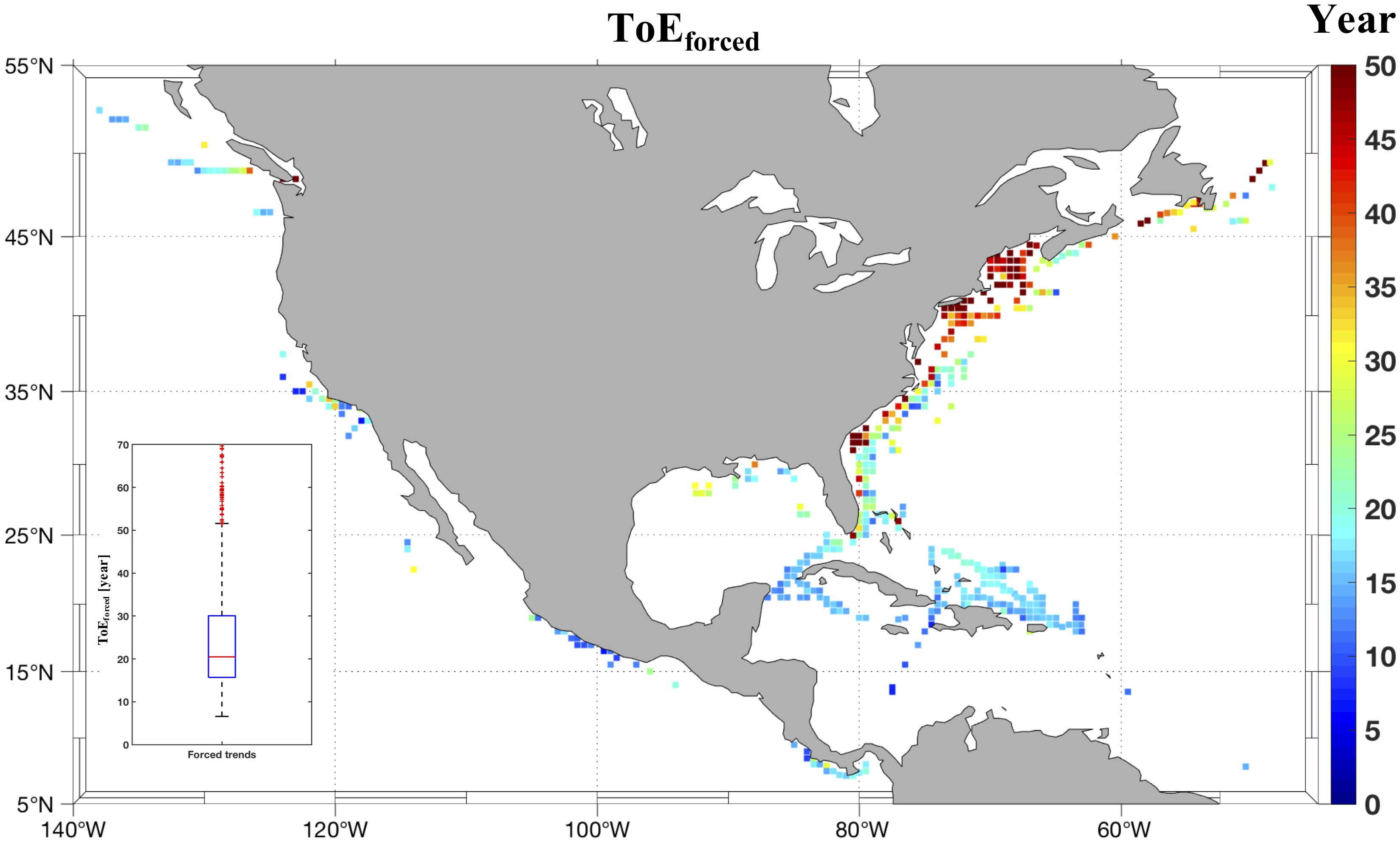
Figure 1. ToE_forced of f(CO_2,sw) in the North American coastal margins. The inserted panel is the boxplot of ToE [the red line inside the blue rectangle (the interquartile range) represents the median, the “whiskers” above and below the rectangle show the minimum and maximum ToE values, and the red crosses are the outliers].

FIGURE 2

Figure 2. ToE_obs of f(CO_2,sw) in the North American coastal margins. Note, the pentagram symbols highlight the negative trends, and the corresponding ToE represents the absolute value. The inserted panel is the boxplot of ToE [the red line inside the blue rectangle (the interquartile range) represents the median, the “whiskers” above and below the rectangle show the minimum and maximum ToE values, and the red crosses are the outliers].

ToE in the Coastal Margins vs. Open Ocean

In agreement with previous estimates of ToE of OA variables in costal margins (Sutton et al., 2018), our results suggest that the average ToE of surface f(CO_2,sw) in ocean margins is greater (>20 years) than in the open ocean. Ocean margins are subjected to multiple forcings that can confound the f(CO_2,sw) increase caused by atmospheric CO₂ accumulation alone and therefore a longer time-series observation may be needed to detect the OA in comparison to the open ocean, unless efforts are made to deconvolute the various contributing processes. Nevertheless, ToE for f(CO_2,sw) is shorter than that for SST (80.4 ± 49.4 years), consistent with previous studies in the open ocean (Christian, 2014; Keller et al., 2014; Rodgers et al., 2015; Henson et al., 2016, 2017). This is not surprising, considering that CO₂/OA are being directly forced anthropogenically through increasing atmospheric CO₂ concentrations (past centuries), changes in physical oceanographic forcing such as upwelling (recent decades), or nutrient increase (recent decades). SST instead reacts to the CO₂ increase induced by climate change, and thus the magnitude of the trend signal will be smaller (Keller et al., 2014).

Main Findings and Recommendations

Main Findings

• Based on data currently included in SOCAT V5 coastal database and assuming a forced trend, the theoretical timeframe (ToE_forced) within which the OA signal in f(CO_2,sw) will emerge in the North American coastal margins, is 23 ± 13 years on average. This result should be interpreted as an ideal case, whereby the secular trend is solely driven by atmospheric CO₂ invasion amid natural background variability. However, there is considerable fine-scale spatial variability with significantly lower values (<20 years) along the west coast and the Caribbean Sea, while it may take east coast waters 30 years or longer to express OA conditions outside natural variability.

• Less than 30% of the grids provided significant observed f(CO_2,sw) trends, primarily reflecting gaps in the current SOCAT database, or data records of insufficient length, to exhibit the trend. ToE based on these observed trends (ToE_obs) was on average 5 years longer than ToE_forced, implying that most coastal areas are experiencing antagonistic secular and/or multi-decadal forcing that dampen the OA signal (notable exceptions are apparent).

• Overall, both ToE_obs and ToE_forced of surface f(CO_2,sw) in the North American ocean margins (23 ± 13 and 28.7 ± 20.4 years, respectively) are higher than that in the open ocean (<20 years). Large regional differences suggest the influence of long-term non-OA processes (e.g., warming, eutrophication, enhanced primary productivity, and increased upwelling) that may not be sufficiently resolved by current observations.

Recommendations

• ToE_forced and ToE_obs values suggest that locations along North American west coast will likely express an anthropogenic OA signal sooner, and therefore are suitable places for OA signal detection in the next few decades. At east coast locations with longer ToEs, other forcings may counteract f(CO_2,sw) change. Continuation of time-series observations, which include a comprehensive suite of measurements and/or coupled with targeted process investigations that allow for specific discrimination of the different forcing processes, is needed at these locations to better assess if the observed trends persist and better discern the OA signal.

• In many instances, we cannot expect that the OA signal is currently detectable directly from observing assets. Longer coastal time-series and the integration of multidisciplinary data from SOCAT, Global Ocean Data Analysis Project (GLODAP), Volunteer Observing Ship (VOS), in situ moorings and remote sensing are needed to provide better estimates of ToE_obs for f(CO_2,sw) and other OA variables (pH and aragonite saturation states), in order to develop proxies of ToE in areas of limited observations. Closer collaborations between multidisciplinary time-series programs and modelers, who use the observations and coastal modeling that more comprehensively account for the range of coastal biogeochemical processes, are also urgently needed to support decision making tools.

• Further review of methodology for the calculation of trends and variability, to address challenges such as seasonal sampling bias, original vs. detrended data, and use of arbitrary specified threshold (N), is needed. N represents a qualitative assessment of when we suspect the environment experienced by the marine organisms is “noticeably” different. N is most likely species dependent and may vary between different regions, especially if vulnerabilities of organisms are taken into consideration. Studies that will provide better estimates of what a meaningful threshold might be for a specified application are therefore needed. Defining best practices for calculating ToE and standardization of OA measurements is recommended.

• A similar ToE analysis as presented here is recommended for other EOVs in support of designing a new multi-purpose (beyond OA detection) observing system, or augmenting an existing one, to ensure that an optimal set of measurements is included, and the appropriate time frame is planned for.

• Consideration of information such as presented here by the UN Decade of Ocean Science for Sustainable Development (2021–2030) in areas of synthesizing existing research, defining trends, knowledge gaps and priorities for future research, and providing science-based information to inform managers and policy makers, is recommended. Therefore, there is still a tremendous need for long-term support from funding agencies, as well as initiatives and leadership from both within the oceanographic community and beyond.

Data Availability

Publicly available datasets were analyzed in this study. These data can be found here: https://www.socat.info.

Author Contributions

DG provided the initial idea for the topic addressed. HW performed the statistical analysis. DT led writing of the manuscript. DT, HW, XH, DG, ZW, LJ, and W-JC contributed to the development, writing, and proofing of this manuscript.

Funding

HW was partially supported by an NSF grant (OCE#1654232) while being a research associate at TAMUCC.

Conflict of Interest Statement

The authors declare that the research was conducted in the absence of any commercial or financial relationships that could be construed as a potential conflict of interest.

Acknowledgments

We are grateful to Charles Kovach for editorial help and the Ocean Carbon & Biogeochemistry (OCB) Project Office (Heather Benway) for helpful input during the development of an initial idea for this study at the 4th U.S. OA PI meeting sponsored by NSF, NOAA, and NASA. We thank two reviewers and the editor for their insight and comments that improved the manuscript. Lamont-Doherty Earth Observatory contribution number 8290.

References

Bakker, D. C., Pfeil, B., Landa, C. S., Metzl, N., O’brien, K. M., Olsen, A., et al. (2016). A multi-decade record of high-quality fCO₂ data in version 3 of the surface ocean CO₂ atlas (SOCAT). Earth Syst. Sci. Data 8, 383–413. doi: 10.5194/essd-8-383-2016

CrossRef Full Text | Google Scholar

Bates, N. R. (2017). Twenty years of marine carbon cycle observations at devils hole bermuda provide insights into seasonal hypoxia, coral reef calcification, and ocean acidification. Front. Mar. Sci. 4:36. doi: 10.3389/fmars.2017.00036

CrossRef Full Text | Google Scholar

Carter, B. R., Frölicher, T. L., Dunne, J. P., Rodgers, K. B., Slater, R. D., and Sarmiento, J. L. (2016). When can ocean acidification impacts be detected from decadal alkalinity measurements? Global Biogeochem. Cycles 30, 595–612. doi: 10.1002/2015GB005308

CrossRef Full Text | Google Scholar

Christian, J. R. (2014). Timing of the departure of ocean biogeochemical cycles from the preindustrial state. PLoS One 9:e109820. doi: 10.1371/journal.pone.0109820

PubMed Abstract | CrossRef Full Text | Google Scholar

Dai, M., Lu, Z., Zhai, W., Chen, B., Cao, Z., Zhou, K., et al. (2009). Diurnal variations of surface seawater pCO₂ in contrasting coastal environments. Limnol. Oceanogr. 54, 735–745. doi: 10.4319/lo.2009.54.3.0735

CrossRef Full Text | Google Scholar

Dore, J. E., Lukas, R., Sadler, D. W., Church, M. J., and Karl, D. M. (2009). Physical and biogeochemical modulation of ocean acidification in the central North Pacific. Proc. Natl. Acad. Sci. U.S.A. 106, 12235–12240. doi: 10.1073/pnas.0906044106

PubMed Abstract | CrossRef Full Text | Google Scholar

Duarte, C. M., Hendriks, I. E., Moore, T. S., Olsen, Y. S., Steckbauer, A., Ramajo, L., et al. (2013). Is ocean acidification an open-ocean syndrome? Understanding anthropogenic impacts on seawater pH. Estuaries Coast. 36, 221–236.

Google Scholar

Fennel, K., Alin, S., Barbero, L., Evans, W., Bourgeois, T., Cooley, S., et al. (2018). Carbon cycling in the North American coastal ocean: a synthesis. Biogeosci. Discuss. doi: 10.5194/bg-2018-420

Frankignoulle, M., and Borges, A. (2001). The european continental shelf as a significant sink for atmospheric carbon dioxide. Global Biogeochem. Cycles 15, 569–576. doi: 10.1029/2000GB001307

CrossRef Full Text | Google Scholar

Friedrich, T., Timmermann, A., Abe-Ouchi, A., Bates, N. R., Chikamoto, M. O., and Church, M. J. (2012). Detecting regional anthropogenic trends in ocean acidification against natural variability. Nat. Clim. Change 2, 167–171. doi: 10.1038/nclimate1372

CrossRef Full Text | Google Scholar

Frölicher, T. L., Rodgers, K., Stock, C., and Cheung, W. W. L. (2016). Sources of uncertainties in 21st century projections of potential ocean ecosystem stressors. Global Biogeochem. Cycles 30, 1224–1243.

Google Scholar

Guo, X., Dai, M., Zhai, W., Cai, W.-J., and Chen, B. (2009). CO2 flux and seasonal variability in a large subtropical estuarine system, the pearl river estuary, china. J. Geophys. Res. 114:G03013. doi: 10.1029/2008JG000905

CrossRef Full Text | Google Scholar

Hawkins, E., and Sutton, R. (2012). Time of emergence of climate signals. Geophys. Res. Lett. 39:L01702. doi: 10.1029/2011GL050087

CrossRef Full Text | Google Scholar

Heinze, C., Ilyina, T., and Gehlen, M. (2018). The potential of 230Th for detection of ocean acidification impacts on pelagic carbonate production. Biogeosciences 15, 3521–3539. doi: 10.5194/bg-15-3521-2018

CrossRef Full Text | Google Scholar

Henson, S. A., Beaulieu, C., Ilyina, T., John, J. G., Long, M., Séférian, R., et al. (2017). Rapid emergence of climate change in environmental drivers of marine ecosystems. Nat. Commun. 8:14682. doi: 10.1038/ncomms14682

PubMed Abstract | CrossRef Full Text | Google Scholar

Henson, S. A., Beaulieu, C., and Lampitt, R. (2016). Observing climate change trends in ocean biogeochemistry: when and where. Global Change Biol. 22, 1561–1571. doi: 10.1111/gcb.13152

PubMed Abstract | CrossRef Full Text | Google Scholar

Hofmann, G. E., Smith, J. E., Johnson, K. S., Send, U., Levin, L. A., Micheli, F., et al. (2011). High-frequency dynamics of ocean pH: a multi-ecosystem comparison. PLoS One 6:e28983. doi: 10.1371/journal.pone.0028983

PubMed Abstract | CrossRef Full Text | Google Scholar

Huang, W.-J., Cai, W.-J., Wang, Y., Lohrenz, S. E., and Murrell, M. C. (2015). The carbon dioxide system on the mississippi river-dominated continental shelf in the northern gulf of Mexico: 1. Distribution and air-sea CO2 flux. J. Geophys. Res. Oceans 120, 1429–1445. doi: 10.1002/2014JC010498

PubMed Abstract | CrossRef Full Text | Google Scholar

Ilyina, T., Zeebe, R. E., Maier-Reimer, E., and Heinze, C. (2009). Early detection of ocean acidification effects on marine calcification. Global Biogeochem. Cycles 23:GB1008. doi: 10.1029/2008GB003278

PubMed Abstract | CrossRef Full Text | Google Scholar

Ishii, M., Kosugi, N., Sasano, D., Saito, S., Midorikawa, T., and Inoue, H. Y. (2011). Ocean acidification off the south coast of Japan: a result from time series observations of CO₂ parameters from 1994 to 2008. J. Geophys. Res. 116:C06022. doi: 10.1029/2010JC006831

CrossRef Full Text | Google Scholar

Kapsenberg, L., and Hofmann, G. E. (2016). Ocean pH time-series and drivers of variability along the northern channel islands, California, USA. Limnol. Oceanogr. 61, 953–968.

Google Scholar

Keller, K. M., Joos, F., and Raible, C. C. (2014). Time of emergence of trends in ocean biogeochemistry. Biogeosciences 11, 3647–3659.

Google Scholar

Landschützer, P., Gruber, N., Bakker, D. C. E., Schuster, U., Nakaoka, S., Payne, M. R., et al. (2013). A neural network-based estimate of the seasonal to inter-annual variability of the atlantic ocean carbon sink. Biogeosciences 10, 7793–7815.

Google Scholar

Laruelle, G. G., Cai, W.-J., Hu, X., Gruber, N., Mackenzie, F. T., and Regnier, P. (2018). Continental shelves as a variable but increasing global sink for atmospheric carbon dioxide. Nat. Commun. 9:454. doi: 10.1038/s41467-017-02738-z

PubMed Abstract | CrossRef Full Text | Google Scholar

Lyu, K., Zhang, X., Church, J. A., Slangen, A. B. A., and Hu, J. (2014). Time of emergence for regional sea-level change. Nat. Clim. Change 4, 1006–1010. doi: 10.1038/nclimate2397

PubMed Abstract | CrossRef Full Text | Google Scholar

Mahlstein, I., Hegerl, G., and Solomon, S. (2012). Emerging local warming signals in observational data. Geophys. Res. Lett. 39, L21711.

Google Scholar

Majkut, J. D., Sarmiento, J. L., and Rodgers, K. B. (2014). A growing oceanic carbon uptake: results from an inversion study of surface pCO2 data. Global Biogeochem. Cycles 28, 335–351.

Google Scholar

McKinley, G. A., Pilcher, D. J., Fay, A. R., Lindsay, K., Long, M. C., and Lovenduski, N. S. (2016). Timescales for detection of trends in the ocean carbon sink. Nature 530, 469–472. doi: 10.1038/nature16958

PubMed Abstract | CrossRef Full Text | Google Scholar

Miloslavich, P., Bax, N. J., Simmons, S. E., Klein, E., Appeltans, W., Aburto-Oropeza, O., et al. (2018). Essential ocean variables for global sustained observations of biodiversity and ecosystem changes. Global Change Biol. 24, 2416–2433. doi: 10.1111/gcb.14108

PubMed Abstract | CrossRef Full Text | Google Scholar

O’Brien, T. (2018). Indicator: Ocean Chlorophyll Concentrations. Available at https://data.globalchange.gov/report/indicator-ocean-chlorophyll-concentrations-2018

Google Scholar

Reimer, J. J., Wang, H., Vargas, R., and Cai, W.-J. (2017). Multidecadal fCO2 increase along the united states southeast coastal margin. J. Geophys. Res. Oceans 122, 10061–10072.

Google Scholar

Rodgers, K., Lin, J., and Frolicher, T. L. (2015). Emergence of multiple ocean ecosystem drivers in a large ensemble suite with an Earth system model. Biogeosciences 12, 3301–3320.

Google Scholar

Salisbury, J. E., and Jönsson, B. F. (2018). Rapid warming and salinity changes in the gulf of maine alter surface ocean carbonate parameters and hide ocean acidification. Biogeochemistry 141, 401–418. doi: 10.1007/s10533-018-0505-3

CrossRef Full Text | Google Scholar

Sutton, A. J., Feely, R. A., Maenner-Jones, S., Musielwicz, S., Osborne, J., Dietrich, C., et al. (2018). Autonomous seawater pCO₂ and pH time series from 40 surface buoys and the emergence of anthropogenic trends. Earth Syst. Sci. Data Discuss. doi: 10.5194/essd-2018-114

CrossRef Full Text | Google Scholar

Vandemark, D., Salisbury, J. E., Hunt, C. W., Shellito, S. M., Irish, J. D., McGillis, W. R., et al. (2011). Temporal and spatial dynamics of CO₂ air-sea flux in the gulf of maine. J. Geophys. Res. 116:C01012. doi: 10.1029/2010JC006408

CrossRef Full Text | Google Scholar

Wang, H., Hu, X., Cai, W.-J., and Sterba-Boatwright, B. (2017). Decadal fCO2 trends in global ocean margins and adjacent boundary current-influenced areas. Geophys. Res. Lett. 44, 8962–8970. doi: 10.1002/2017GL074724

CrossRef Full Text | Google Scholar

Wang, H., Hu, X., and Sterba-Boatwright, B. (2016). A new statistical approach for interpreting oceanic fCO₂ data. Mar. Chem. 183, 41–49. doi: 10.1016/j.marchem.2016.05.007

CrossRef Full Text | Google Scholar

Wootton, J. T., and Pfister, C. A. (2012). Carbon system measurements and potential climatic drivers at a site of rapidly declining ocean pH. PLoS One 7:e53396. doi: 10.1371/journal.pone.0053396

PubMed Abstract | CrossRef Full Text | Google Scholar