Sediment-Associated Phytoplankton Release From the Seafloor in Response to Wind-Induced Barotropic Currents in the Bering Strait

Introduction

The continental shelf region of the Chukchi and Bering seas is experiencing a rapid decline in sea ice extent and changes in water mass property, which can cause a shift in marine species composition and carbon cycling (Grebmeier et al., 2015). This region is considered to be one of the most biologically productive regions in the world. The high primary production is sustained by the advective supply of nutrient-rich Anadyr water from the south (Springer and McRoy, 1993). Massive spring phytoplankton blooms in surface water produce a substantial amount of organic matter, which is transported downward; most of this organic matter reaches the seafloor without being consumed by zooplankton in the water column by tight pelagic–benthic coupling (Grebmeier et al., 1988). The accumulated organic matter is then consumed by benthic organisms (e.g., bivalves and amphipods), creating so-called biological hotspots (Grebmeier et al., 2015). The southeastern Chukchi Sea, which is located in the downstream region of the Bering Strait throughflow, receives horizontal inputs of particulate organic matter and nutrients from the south (Grebmeier et al., 2015; Nishino et al., 2016). Potential horizontal transport pathways include resuspended sediments in epibenthic water and the suspended organic matter in surface water.

The Bering Strait throughflow, driven by the sea-level differences between the Bering and Chukchi Seas, is primarily northward; in addition, the throughflow can exceed 100 cm s^-1 by local winds (Roach et al., 1995). The moored current meter observations and ocean model indicated that the Bering Strait exhibited the largest ocean current variability in the Bering and Chukchi Seas (Danielson et al., 2014; Pisareva et al., 2015). The statistics summarized by Grebmeier et al. (2015) indicated that the standard deviation of northward current in the Bering Strait is 2–4 times of that in the northern Bering and eastern Chukchi Seas. Another important feature of the Bering Strait throughflow is the strongly uniform and mostly barotropic (i.e., invariant with depth) current, except for that in the eastern boundary region (Woodgate et al., 2015). Intense friction velocities in the bottom layer would induce resuspension of the seafloor sediment. The sediment contains relatively fresh organic matter, as indicated by the particulate organic carbon/particulate nitrogen (C/N) ratio (wt/wt: 6.26) and chlorophyll concentrations (15.74 mg chl. a m^-2) near the Bering Strait during both spring and summer (Grebmeier et al., 2015). If sediment dispersion occurs, the resuspended particles, organic matter, and nutrients can be horizontally transported to the north. The sediment dispersion that may occur in the Bering Strait could significantly affect the formation of biological hotspots in the northern Bering Sea/southern Chukchi Sea.

Woodgate et al. (2015) reported that the volume transport in the Bering Strait exhibits an increasing trend, with a 50% increase in 2013 as compared to that observed in 2001. Because the magnitude of sediment particle dispersion depends on the near-bottom current velocity, understanding the linkage of the physical and biological processes that may occur at the bottom of the Bering Strait attains an ever-increasing importance. However, to the best of our knowledge, this point has not been studied thus far.

Therefore, we conducted in situ observations from September 2016 to July 2017 using an instrument-outfitted mooring. Data were collected using the turbidity and chlorophyll fluorescence sensors as well as an acoustic doppler current profiler (ADCP) mounted on the mooring; these data helped in quantifying the physical–biological linkage. We investigated (a) whether this strong current contributes to the resuspension of sediment-associated phytoplankton and organic matter and (b) how the current is linked to the surface wind and atmospheric forcing.

Materials and Methods

The mooring was positioned close to mid-channel ∼35 km north of the narrowest part of the Bering Strait (Figure 1; 66°16.046′N, 168°54.016′W; ∼58-m deep). This location is close to the mooring site of Woodgate et al. (2005a) that is referred to as A3 site (see Figure 1 of their study). At this location, warm, fresh, and nutrient-poor Alaskan Costal Current flowing in the east, and cold, high-salinity, and nutrient-rich Anadyr water flowing in the west meet and combine, yielding a useful average of physical water properties in the Bering Strait (Woodgate and Aagaard, 2005; Woodgate et al., 2005a, 2006, 2007, 2015).

FIGURE 1

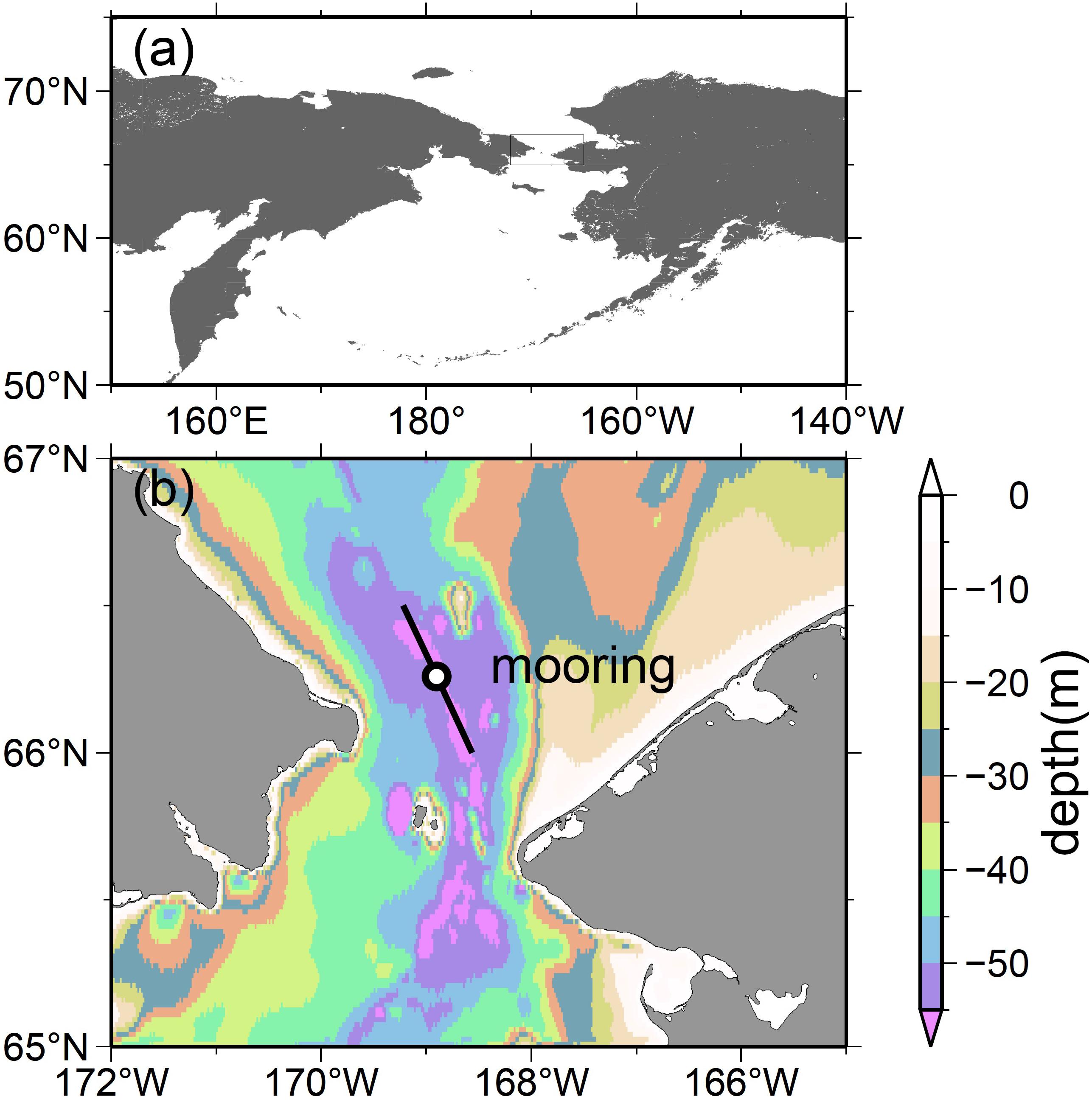
Figure 1. Maps of the research area. The inset rectangle in (a) indicates the region of an enlarged map (b). The black circle in (b) represents the mooring site (66°16.046′N, 168°54.016′W). The solid line denotes the principal axis of the near-bottom velocity measured using an ADCP, as depicted in Figure 2. The colors indicate the continental shelf region’s bathymetry based on ETOPO1 (Amante and Eakins, 2009). The bottom depth at the mooring site is ∼58 m.

The mooring-collected chlorophyll a (chl. a) concentration and turbidity data are obtained 3 m above the seafloor using a fluorescence and turbidity sensor, INFINITY ACLW2-USB (JFE Advantech). The fluorescence and turbidity sensor possesses a mechanical wiper that periodically cleans the sensor’s surface at 30-min intervals to inhibit biological contamination on the optical window immediately before a burst of measurements¹. This sensor-derived chl. a concentration was calibrated using the extracted chl. a concentration of the water sample obtained at the same station during mooring recovery (4.0 mg m^-3), which revealed that the sensor had slightly overestimated the concentration (4.5 mg m^-3) before calibration. Also, another seawater sample taken during mooring deployment (3.5 mg m^-3) quantitatively supported this sensor-derived calibrated chl. a concentration (2.0 mg m^-3) as well, although the sampling depth was 7 m shallower than the sensor depth. Pigments on a filter sample were extracted with N, N-dimethylformamide (DMF) (Suzuki and Ishimaru, 1990). Chl. a in seawater samples was measured using a fluorometric non-acidification method (Welshmeyer, 1994) with a Turner Design fluorometer (10-AU-005; Sunnyvale, CA, United States). The linear response of the fluorescence sensor to liquid fluorescent standard is verified via laboratory testing in the manufacture stage.

The data also included velocity data and echo intensity measured 3 m above the seafloor using a Workhorse ADCP 300 kHz SC Sentinel (Teledyne RD Instruments Inc., 2007). At 30-min intervals, the ADCP sampled the vertical velocity profile at 4-m intervals with 15 bins, except for the deepest bin whose size is 6 m. This ADCP also sampled acoustic pulses transmitted by the ADCP transducer. As reported by Ito et al. (2017), the pulses are scattered by the suspended particles in the overlaying water column [unit is Workhorse ADCP count, which is equivalent to ∼0.45 dB (Deines, 1999)]. Although the received echo intensity depends on the distance from the transducer to scatterers, because of geometric spreading of the acoustic beam, and because of sound absorption by the water (Ito et al., 2017), we only discuss the scatter density over time at particular depths, and compare the coherency of the signal strength over different depths. Among the 15 bins, the data in the top 4 bins were not used because the echo intensity indicated that these bins were considerably close to the sea surface. Using the mooring’s built-in compass, we corrected the current direction to the geographical north based on the 12th generation International Geomagnetic Reference Field (Thébault et al., 2015). We applied the 24-h block average to the near-bottom fluorescence–turbidity measurements and the profile data from the ADCP for obtaining daily data. Although the averaging process aliases several tidal frequencies, it also minimizes the unwanted signature of high-frequency tidal currents. We considered this negative impact to be negligible because Woodgate et al. (2005b) showed that the tidal currents at this location are very small (<2 cm s^-1).

To estimate the chl. a concentration in surface water, we obtained the MODIS/Aqua standard mapped images of remote sensing reflectance at 443, 488, and 555 nm at 9-km resolution from the NASA Goddard Space Flight Center’s Distributed Active Archive Center. We employed the modified version of the Arctic-OC4L algorithm (Fujiwara et al., 2016). This regionally optimized retrieval algorithm with focus on the Pacific–Arctic region reduces the overestimation of chl. a concentration in the Chukchi Sea owing to the presence of highly concentrated chromophoric dissolved organic matter supplied by river inputs (Wang and Cota, 2003; Cota et al., 2004; Matsuoka et al., 2007; Mustapha et al., 2012). Furthermore, we ensured that the results presented herein do not depend on different choices of the product by comparing the product obtained using the Arctic-OC4L algorithm with a product obtained using another algorithm independently developed by Lewis et al. (2016) (not shown).

We downloaded sea ice concentration data retrieved from passive microwave observations by the Advanced Microwave Scanning Radiometer-2/Global Change Observation Mission-W from JAXA. This sea ice concentration product was generated based on a bootstrap algorithm (Comiso et al., 2003) using three frequency channels (18.7, 22, and 36.5 GHz) with a grid spacing of 7 × 12 km.

We also used the surface wind and sea-level pressure (SLP) data provided by the European Center for Medium-Range Weather Forecasts (ECMWF), referred to as Interim ECMWF Re-Analysis (ERA-Interim, Simmons et al., 2010; Dee et al., 2011). The data have a daily frequency in a 0.75° × 0.75° (longitude × latitude) grid.

Results

Current Velocities

Figure 2 shows the northward and eastward components of the current velocities that are measured in the shallowest, middle, and deepest layers. The velocity data obtained from these layers exhibited large variability along the near-bottom regression line. In particular, the data distributions in the middle and deepest layers were observed to be rectilinear, which were in contrast to that of the shallowest layer containing somewhat dispersed data points. Because the regression line was 332° clockwise from the north, the near-bottom current flowed along the north-northwest direction. This was identical to the direction of the depression that extends along the canyon floor (Figure 1), indicating that the rectilinear flow pattern of the near-bottom current resulted from being steered by the seafloor topography around the mooring site. The meridional component ranged from -80 to +100 cm s^-1, whereas the horizontal component ranged from -40 to +60 cm s^-1. The current velocity of more than ±60 cm s^-1 may not be quantitatively reliable owing to the large tilt of the mooring line (not shown), although qualitatively, this large tilt indicates the presence of considerable flow. More than half of the data points were plotted in the region of the positive y axis, indicating that the flows are more likely to be directed northward than southward.

FIGURE 2

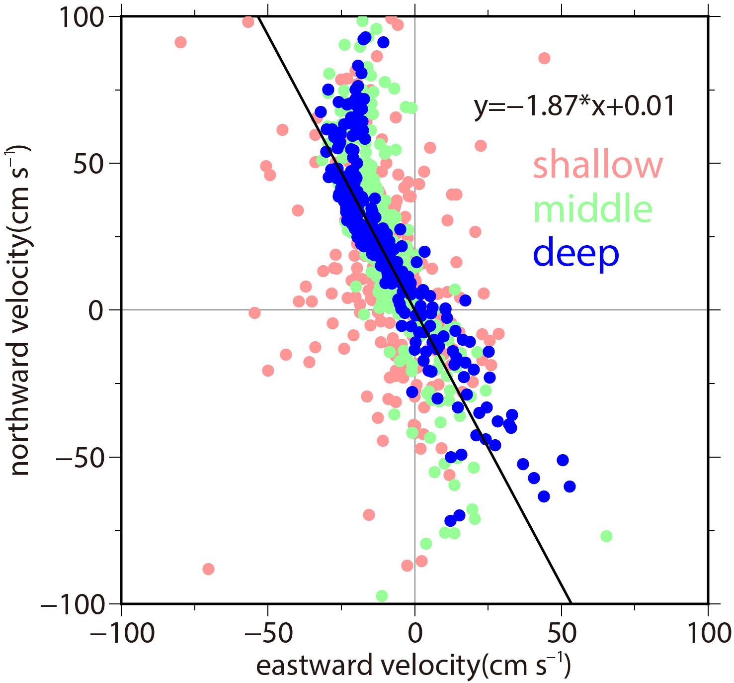
Figure 2. Daily mean ADCP velocities (cm s^-1) in the Bering Strait. The velocities that are measured at the shallowest layer (45–49 m from the bottom), middle layer (25–29 m from the bottom), and deepest layer (3–9 m from the bottom) are indicated by red, green, and blue circles, respectively. Among these layers, only the deepest layer data are used to calculate the regression line (indicated by a solid line). This regression line, which is identical to the y axis rotated 332° clockwise, is used as the principal velocity axis onto which the velocity data are projected for analyzing the major velocity variability.

Hereafter, we only consider the flow’s near-bottom component, which directly affects the sediment resuspension. In addition, we consider this heading angle (332°) to be the principal axis of the flow. The velocity that is projected onto this principal axis is simply referred to as the northward or southward current.

Sediment-Associated Phytoplankton/Organic Matter Release From the Seafloor

Figure 3 shows daily-mean time series of the satellite-observed surface chl. a concentration, near-bottom chl. a concentration and turbidity, the principal component of near-bottom ADCP current velocity, and ECMWF surface winds from 2016 to 2017. The MODIS/Aqua chl. a concentration data frequently exhibited missing values during the fall and winter (Figure 3a) owing to the presence of cloud cover and sea ice. Hereafter, we describe the results in the following order; 2016 fall, 2016 winter, and 2017 spring.

FIGURE 3

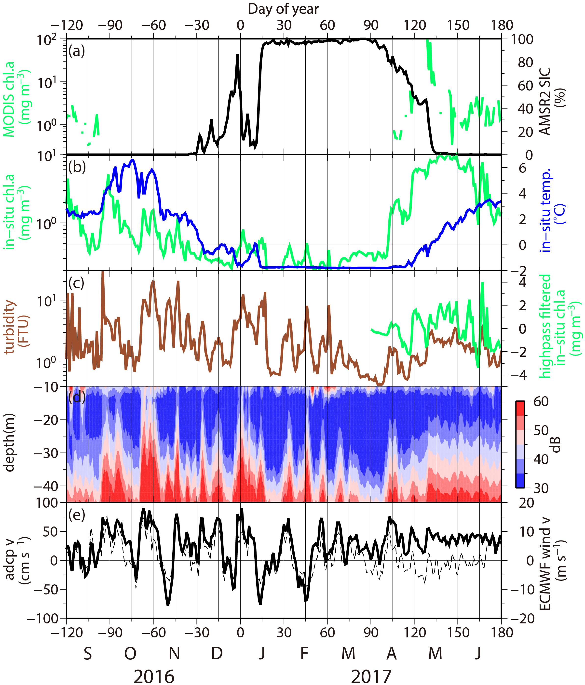
Figure 3. Daily mean time series of the (a) MODIS/Aqua chlorophyll a (chl. a) concentration in surface water (mg m^-3; green line) and AMSR2 sea ice concentration (%; black line), (b) near-bottom chl. a concentration (mg m^-3; green line) and temperature (°C; blue line), (c) turbidity [formazin turbidity unit (FTU); brown line] and high-frequency component of near-bottom chl. a concentration using a high-pass filter with a half-power point of 40 days during the spring, (d) vertical structure of ADCP echo intensity (dB), and (e) principal component of ADCP current velocity (cm s^-1; solid line; positive for northward and negative for southward) and ECMWF surface wind velocity (dashed line) at the mooring site. Day of year represents the day counted from January 01, 2017. The satellite and ECMWF reanalysis data are averaged over a 4°× 4 (longitude × latitude) area centered on the mooring site.

Fall (from -120 to -30 Day of year, September to November) was characterized by the highest near-bottom temperature (5°C or greater). During fall, the near-bottom chl. a concentration (Figure 3b) exhibited peaks on -90, -60, -50, and -40 Day of year. The peak amplitudes exceeded 5 mg m^-3, which was one order of magnitude higher than the amplitudes in the subsequent winter. Similarly, the turbidity data (Figure 3c) exhibited the same number of peaks [10 formazin turbidity unit (FTU) or greater], whose timing corresponded to high chl. a concentration event peaks (r = +0.41; Table 1). The simultaneous occurrences of high-turbidity and chl. a concentration events, together with the presence of chl. a in the sediments (100.4 ± 16.7 mg m^-2; n = 4: Waga unpublished data), could indicate that the phytoplankton in the near-bottom water originated from the sea bottom.

TABLE 1

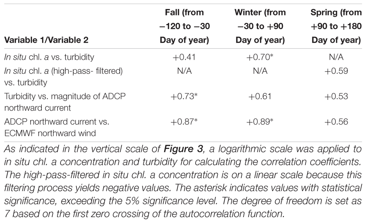
Table 1. Correlation coefficients between variables 1 and 2 during each season.

The vertical structure of the suspended particles that can be inferred from the ADCP echo intensity is shown in Figure 3d. The backscattering signals were generally strong in the lower layers and weak in the upper layers as mentioned in the section “Materials and Methods.” In addition, the intensity of the backscattering signal exhibited short-term variability. In the aforementioned turbidity events, the higher level of echo intensity was discernible even in the upper layers, particularly during -60 Day of year, when the impact of the bottom turbidity reached the near-surface layer.

High-turbidity events were detected under turbulent seafloor conditions (Figure 3e). The events on -90, -60, and -40 Day of year occurred under northward currents (ranging from +70 to +100 cm s^-1), whereas the event on -50 Day of year occurred under a southward current (-80 cm s^-1). The data revealed that the turbidity events could occur in both current directions. The near-bottom velocity magnitude exhibited a significant correlation with the turbidity plume magnitude (r = +0.73, exceeding the 5% significance level). Thus, the frictional velocity in the boundary layer is deemed an important factor that controls the dispersion of the phytoplankton-containing sediment.

Furthermore, this near-bottom current was modulated by surface winds, with the near-bottom current velocity exhibiting a significant correlation with the ECMWF surface winds (dashed line in Figure 3e, r = +0.87, exceeding the 5% significance level). This correlation clearly indicated that the northward surface winds intensified the northward near-bottom ocean currents, and the same is true for southward winds and currents, which is consistent with the results obtained by Danielson et al. (2014).

Next, we focus on winter (from -30 to +90 Day of year; from December to March) when the near-bottom retains the freezing temperature T_f at -1.8°C, i.e., the mooring measures under-ice properties. Basically, we detected similar sediment dispersion under turbulent seafloor conditions during winter as well (see the correspondence of timing with respect to chl. a concentration, turbidity, current, and wind events on +5, +15, +35, +45, and +60 Day of year). The difference was that the increase in chl. a concentration was substantially smaller (<1 mg m^-3) during winter.

During spring (from +90 to +180 Day of year; from April to June), the fluorescence sensor detected a seasonal chl. a concentration event in the near-bottom layer, whose timescale was considerably longer than that of the sediment’s resuspension from the seafloor (Figure 3b). The near-bottom chl. a concentration gradually increased over time (from +100 to +130 Day of year), reaching a peak value of 10 mg m^-3, which was the largest value of our year-round observation, on +140 Day of year. This high value persisted for 20 days before a decreasing phase was observed from +160 Day of year. This event occurred in phase with the near-surface spring phytoplankton bloom (Figure 3a), which exhibited a distinct sharp peak on +130 to +135 Day of year, equivalent to mid May, when the near-bottom temperature started to increase (Figure 3b) and the AMSR2 sea ice concentration rapidly decreased from 100 to 0% (Figure 3a). The timing is 1 month earlier than during a normal year (Fujiwara et al., 2016), or during the same time as the bloom timing of 2003 estimated via direct observations in surface waters of the Bering Strait (Cooper et al., 2006).

To extract the sediment resuspension signature, we applied a high-pass filter to the bloom-contaminated data. The filtered short-term variability (Figure 3c) denoted distinct peaks on +105, +120, +155, and +165 Day of year. The timing of these short-term phytoplankton events was consistent with the timing of springtime turbidity events (r = +0.59; Table 1). The turbidity event amplitudes were weaker than those in fall and winter because the near-bottom current and surface winds were also weak. However, the correlation coefficients between turbidity and near-bottom current velocity (r = +0.53) and those between current velocity and wind speed (r = +0.56) exhibited an insignificant but high positive correlation.

Atmospheric Pressure Field

In this subsection, we examine the spatial and temporal scales of the atmospheric forcing driving/modulating barotropic currents in the Bering Strait. The winds over the Bering and Chukchi Seas depend on the time-varying strength and position of the Siberian and Beaufort highs and the Aleutian low atmospheric pressure systems (Danielson et al., 2014). Figure 4 shows the regressions of ECMWF SLP and wind velocity onto the near-bottom ADCP velocity [hPa (m s^-1)^-1]. These maps represent the anomalous SLP and wind fields when the anomalous near-bottom flow is northward at a speed of +100 cm s^-1. At a lead–lag value of -3 days (i.e., SLP leads the northward current), a dipole pattern of SLP anomalies emerged with negative SLP anomalies over Siberia and positive SLP anomalies over Alaska. At a lead–lag value of 0 days, this dipole pattern was remarkably enhanced in amplitude, and strong northward winds of more than 10 m s^-1 were observed to blow over the Bering and Chukchi Seas, which were substantially weakened at a lead–lag value of +3 days. Northward currents in the Bering Strait were modulated by surface winds associated with an intercontinental atmospheric pattern having a 5000-km spatial scale for 6 days. This result was not sensitive to data analysis performed in different seasons (not shown).

FIGURE 4

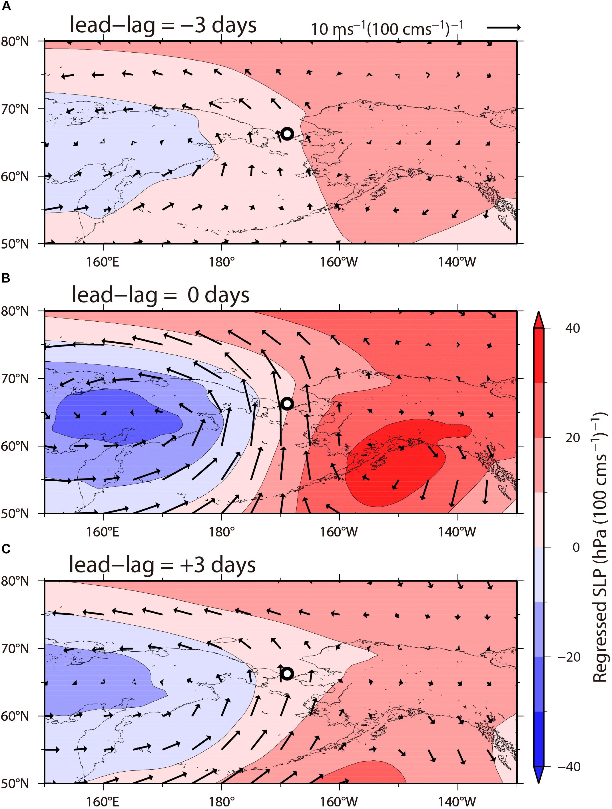
Figure 4. The lead–lag regression of the ECMWF sea-level pressure [SLP, color; hPa (100 cm s^-1)^-1] and wind velocity [arrows; m s^-1 (100 cm s^-1)^-1] onto the near-bottom ADCP principal component velocity at the mooring site. Lead–lag values are (A) -3 days, (B) 0 days, and (C) +3 days. The daily lead–lag value is negative (positive) when the SLP leads (lags) the ADCP velocity. The black circle denotes the mooring site.

Discussion

The wind-induced near-bottom currents can be intensified up to 100 cm s^-1 (Figure 3e). As suggested by Danielson et al. (2014), the ocean current response to wind forcing in the Bering Strait is locally strong over the Bering and Chukchi Seas. This can be attributed to the unique geographic feature of the Bering Strait in which the Bering Strait throughflow is accelerated when it passes through the narrowest part of the strait (80 km).

This strong wind-driven current having an intensity of 70–100 cm s^-1 induces the resuspension of sediment-associated phytoplankton and organic matter from the seafloor during all seasons. The phytoplankton/organic matter dispersion response to wind-induced currents was seasonal, with large increases during the fall and spring and small increases during winter. The occurrence of small wintertime increases can be attributed to the small amounts of fresh phytoplankton and/or phytodetritus cells contained in the sediment during winter when compared to that contained during fall. The phytoplankton deposited in the sediment would have been decomposed by bacteria under warm water conditions during fall, with the half-life of chl. a in the sediment being 35 days in 5°C water (Sun et al., 1993), and during winter when the bacteria are still active even in the cold Arctic water (Garneau et al., 2008). Furthermore, a fresh supply of phytoplankton cells from the overlaying water column is not expected because primary production is less active under sea ice cover during the polar winter. Depending on the physical and biochemical conditions in the sediment, some chl a may exhibit lengthy persistence in Arctic sediments (Pirtle-Levy et al., 2009).

The seafloor discharges the phytoplankton and organic matter via the dispersion, whereas the seafloor charges fresh phytoplankton and organic matter produced in and falling from the surface water during spring phytoplankton bloom and possibly during fall bloom. This charge/discharge process, along with horizontal transport, would play an important role in sustaining biomass around the Bering Strait. The dispersed organic matter/phytoplankton can reach the near-surface layer (Figure 3d). It is possible that these materials are utilized for secondary surface/water column photosynthesis, particularly during the fall (Figure 3b). Further examination is required in the future based on in situ observations. For numerical modeling, when assessing the contribution of sediment resuspension, the relation between turbidity and near-bottom current [log₁₀ (near-bottom turbidity (FTU)) = 0.01098 × (magnitude of near-bottom velocity (cm s^-1)) - 0.132], which is calculated using the least squares method and the daily mean data shown in Figure 3, would be useful for modelers.

Pisareva et al. (2015) indicateed that the seafloor of the Bering Strait contains relatively coarse and medium sand, which is in contrast with the fine sand and silt as well as clay observed in the surrounding region such as the southern Chukchi Sea. In contrast, the annual mean primary production in the Bering Strait is considered to be one order higher than that observed in the surrounding regions. In particular, during spring, this production is substantially higher and the ocean current is weaker, providing a favorable condition for the produced organic matter to accumulate on the seafloor. The high concentration of sediment chl. a is not inconsistent with coarser grained-sized sediments in the Bering Strait.

Our estimation of the sediment chl. a concentrations (100.4 ± 16.7 mg m^-2) is considerably higher than that reported in Grebmeier et al. (2015) (15.74 mg chl. a m^-2). The sampling depth is identical to that reported in Grebmeier et al. (2015) (top 1cm of the sediment); however the organic solvent used to extract pigments from sediments is different. We used N, N-dimethylformamide (DMF) which has higher extraction efficiency than 90% acetone used in Grebmeier et al.’s (2015) work. Furthermore, the location of seawater sampling is not strictly the same in the two studies mentioned above (Bering Strait and Chirikov basin). Although we cannot specify which factor causes this large magnitude difference, these values are in the range of results by McTigue et al. (2015) (10.2–665 mg m^-2) using high-performance liquid chromatography in the Chukchi Sea.

We attempt to quantitatively estimate how much additional material is likely to be imported from the Bering Strait to the southern Chukchi Sea. Data of chl. a concentration measured using the fluorescence sensor is available as a representative of organic matter. Herein, we assume that this resuspension occurs at any location within the Bering Strait, and the consequent profile is vertically homogeneous. The total mass flux of organic matter that passes through the cross section of the Bering Strait, Vol(t) (g day^-1), can be estimated using the following equations;

$$\mathrm{Vol}(\mathrm{t})=\mathrm{chla}(\mathrm{t})\times \mathrm{v}(\mathrm{t})\times \mathrm{L}\times \mathrm{H}$$

where chla (t) is chl. a concentration (g m^-3) and v(t) is northward current velocity (m day^-1), both of which are a function of time t, L is zonal width of the Bering Strait (m), H is vertical level that the resuspended particle reaches from the seafloor (m). The time-varying parameters, chla(t) and v(t), are obtained from the time series shown in Figure 3, H is assumed to be 20 m as the chl. a concentration measured during mooring deployment was homogeneous in this vertical range, and L = 80,000 m is assumed, since as mentioned in the section “Materials and Methods,” this A3 mooring site represents a useful average of the physical water properties in the Bering Strait (Woodgate et al., 2005a). Integration of Vol(t) over major seasons of resuspension (fall and winter, -120 to +90 Day of year, Figure 3), for northward flow v(t) > 0, leads to a total organic matter mass of 3,300 ton chl. a per year.

Travel distance of the organic matter largely depends on the sinking speed. Take diatoms, for example, the sinking speed is in the range of 0.3–17.5 m day^-1 for a diameter of 4–216 μm (Miklasz and Denny, 2010). Suppose the diatoms come up to 20 m from the seafloor through high flow events, which gives the diatoms a residence time of 1–66 days before settling on the seafloor. Calculation of the travel distance using both the residence time and current of 100 cm s^-1 reveals that the diatoms can travel for at least 100 km, thus reaching to biological hotspots in the southeastern Chukchi Sea (Grebmeier et al., 2015; Nishino et al., 2016). Let us make an additional assumption that all dispersed organic matter falls to the seafloor of the biological hotspots, whose area is approximately 60,000 km² = 300 km × 200 km, Figure 2 of Grebmeier et al. (2015). This provides an additional supply of 110 mg chl. a per unit square meter (m^-2) to the sediments, corresponding to 5–6 times of sediment chl. a in the region of biological hotspots (Grebmeier et al., 2015). This relative contribution may be an overestimation as organic matter with less sinking speed can be transported to a wider range of areas. In addition, this total mass flux during fall and winter, which are major seasons of resuspension, may be smaller than that observed in spring bloom season. However, this bottom process that resuspends not only organic matter but also nutrients, would play a significant role in the formation and/or maintenance of the biological hotspots.

The Bering Strait throughflow exhibits a gradually increasing trend over the record length of moored current meter observations from the 1990s (Woodgate et al., 2010, 2015). With increasing current speed, the influence region estimated in the above would expand northward. This may be associated with the recent northward shift of the benthic species reported by Grebmeier et al. (2015). Although the process would not be so simple, the benthic larvae would be transported further north by the greater flow. Regardless, this greater flow would not directly impact the distribution of adult benthos; however, their feeding environment would be changed by the flow.

The present study clearly shows observational evidence that bottom sediments containing phytoplankton cells were resuspended owing to the strong northward bottom current that is driven by strong northward winds in the Bering Strait. Furthermore, the observational evidence may imply that the resuspended sediments are transported northward by the current and an additional source of organic matter fuels benthic/epi-benthic heterotrophs in the southern Chukchi Sea. This observation is expected to contribute to the better forecasting of the marine biological environment in the Arctic Ocean using coupled physical and biological models of marine systems in the future.

Author Contributions

HA, MS, and TH planned the research. HA, MS, and HW analyzed and observed the data. HA and MS prepared first draft of the manuscript. All authors contributed to finalizing the manuscript.

Funding

This study was supported by the Arctic Challenge for Sustainability (ArCS) Project, funded by the Ministry of Education, Culture, Sports, Science, and Technology of Japan (MEXT).

Conflict of Interest Statement

The authors declare that the research was conducted in the absence of any commercial or financial relationships that could be construed as a potential conflict of interest.

Acknowledgments

We thank Editor (AG), Specialty Chief Editor (Dr. Marta Marcos), and the three reviewers who provided valuable comments that contributed to the improvement of this manuscript. We also thank the captains and crews of the T/S Oshoro-Maru and R/V Mirai along with the staff of JAMSTEC and Marine Work Japan, Ltd., for their cooperation during the cruises. We are grateful to Dr. Humio Mitsudera, Dr. Amane Fujiwara, Dr. Eiji Watanabe, Dr. Kohei Matsuno, and Dr. Masato Ito for their fruitful comments and discussions. The ocean color data were provided by the Distributed Active Archive Center at the Goddard Space Flight Center (https://oceancolor.gsfc.nasa.gov/), the sea ice concentration data were provided by JAXA (https://gportal.jaxa.jp/gpr/), the surface wind and SLP data were obtained from ECMWF (http://apps.ecmwf.int/), and the ETOPO1 ocean bathymetry data were provided by the National Oceanic and Atmospheric Administration (https://www.ngdc.noaa.gov/mgg/global/). Finally, we appreciate Enago (http://www.enago.jp) for the English language review.

Footnotes

1. ^https://www.jfe-advantech.co.jp

References

Amante, C., and Eakins, B. W. (2009). ETOPO1 1 Arc-Minute Global Relief Model: Procedures, Data Sources And Analysis. Washington, DC: NOAA Technical Memorandum NESDIS NGDC,

Google Scholar

Comiso, J. C., Cavalieri, D. J., and Markus, T. (2003). Sea ice concentration, ice temperature, and snow depth, using AMSR-E data. IEEE TGRS 41, 243–252. doi: 10.1109/TGRS.2002.808317

CrossRef Full Text | Google Scholar

Cooper, L. W., Codispoti, L. A., Kelly, V., Sheffield, G. G., and Grebmeier, J. M. (2006). The potential for using little Diomede Island as a platform for observing environmental conditions in Bering Strait. Arctic 59, 129–141.

Google Scholar

Cota, G. F., Wang, J., and Comiso, J. C. (2004). Transformation of global satellite chlorophyll retrievals with a regionally tuned algorithm. Remote Sens. Environ. 90, 373–377. doi: 10.1016/j.rse.2004.01.005

CrossRef Full Text | Google Scholar

Danielson, S. L., Weingartner, T. W., Hedstrom, K., Aagaard, K., Woodgate, R., Curchitser, E., et al. (2014). Coupled wind-forced controls of the Bering–Chukchi shelf circulation and the Bering Strait through-flow: Ekman transport, continental shelf waves, and variations of the Pacific–Arctic sea surface height gradient. Prog. Oceanogr. 125, 40–61. doi: 10.1016/j.pocean.2014.04.006

CrossRef Full Text | Google Scholar

Dee, D. P., Uppala, S. M., Simmons, A. J., Berrisford, P., Poli, P., Kobayashi, S., et al. (2011). The ERA-Interim reanalysis: configuration and performance of the data assimilation system. Q. J. R. Meteorol. Soc. 137, 553–597. doi: 10.1002/qj.828

CrossRef Full Text | Google Scholar

Deines, K. L. (1999). Backscatter estimation using broadband acoustic doppler current profilers. Paper Presented at Sixth Working Conference on Current Measurement, San Diego, CA. doi: 10.1109/CCM.1999.755249

CrossRef Full Text | Google Scholar

Fujiwara, A., Hirawake, T., Suzuki, K., Eisner, L., Imai, I., Nishino, S., et al. (2016). Influence of timing of sea ice retreat on phytoplankton size during marginal ice zone bloom period on the Chukchi and Bering shelves. Biogeosciences 13, 115–131. doi: 10.5194/bg-13-115-2016

CrossRef Full Text | Google Scholar

Garneau, M. E., Roy, R. S., Lovejoy, C., Gratton, Y., and Vincent, W. F. (2008). Seasonal dynamics of bacterial biomass and production in a coastal arctic ecosystem: Franklin Bay, western Canadian Arctic. J. Geophys. Res. 113:C07S91. doi: 10.1029/2007JC004281

CrossRef Full Text | Google Scholar

Grebmeier, J. M., Bluhm, B. A., Cooper, L. W., Danielson, S. L., Arrigo, K. R., Blanchard, A. L., et al. (2015). Ecosystem characteristics and processes facilitating persistent macrobenthic biomass hotspots and associated benthivory in the Pacific Arctic. Prog. Oceanogr. 136, 92–114. doi: 10.1016/j.pocean.2015.05.006

CrossRef Full Text | Google Scholar

Grebmeier, J. M., McRoy, C. P., and Feder, H. M. (1988). Pelagic-Benthic Coupling on the Shelf of the Northern Bering and Chukchi Seas. I. Food Supply Source and Benthic Biomass. Fairbanks, AK: Marine Ecology Progress Series, 57–67. doi: 10.3354/meps048057

CrossRef Full Text | Google Scholar

Ito, M., Ohshima, K. I., Fukamachi, Y., Mizuta, G., Kusumoto, Y., and Nishioka, J. (2017). Observations of frazil ice formation and upward sediment transport in the Sea of Okhotsk: a possible mechanism of iron supply to sea ice. J. Geophys. Res. Oceans 122, 788–802. doi: 10.1002/2016JC012198

CrossRef Full Text | Google Scholar

Lewis, K. M., Mitchell, B. G., van Dijken, G. L., and Arrigo, K. R. (2016). Regional chlorophyll a algorithms in the Arctic Ocean and their effect on satellite-derived primary production estimates. Deep Sea Res. Part II 130, 14–27. doi: 10.1016/j.dsr2.2016.04.020

CrossRef Full Text | Google Scholar

Matsuoka, A., Huot, Y., Shimada, K., Saitoh, S. I., and Babin, M. (2007). Bio-optical characteristics of the western Arctic Ocean: implications for ocean color algorithms. Can. J. Remote Sens. 33, 503–518. doi: 10.5589/m07-059

CrossRef Full Text | Google Scholar

McTigue, N. D., Bucolo, P., Liu, Z., and Dunton, K. H. (2015). Pelagic–benthic coupling, food webs, and organic matter degradation in the Chukchi Sea: insights from sedimentary pigments and stable carbon isotopes. Limnol. Oceanogr. 60, 429–445. doi: 10.1002/lno.10038

CrossRef Full Text | Google Scholar

Miklasz, K. A., and Denny, M. W. (2010). Diatom sinking speeds: improved predictions and insight from a modified Stokes’ law. Limnol. Oceanogr. 55, 2513–2525. doi: 10.4319/lo.2010.55.6.2513

CrossRef Full Text | Google Scholar

Mustapha, S. B., Bélanger, S., and Larouche, P. (2012). Evaluation of ocean color algorithms in the southeastern Beaufort Sea, Canadian Arctic: new parameterization using SeaWiFS, MODIS, and MERIS spectral bands. Can. J. Remote Sens. 38, 535–556. doi: 10.5589/m12-045

CrossRef Full Text | Google Scholar

Nishino, S., Kikuchi, T., Fujiwara, A., Hirawake, T., and Aoyama, M. (2016). Water mass characteristics and their temporal changes in a biological hotspot in the southern Chukchi Sea. Biogeosciences 13, 2563–2578. doi: 10.5194/bg-13-2563-2016

CrossRef Full Text | Google Scholar

Pirtle-Levy, R., Grebmeier, J. M., Cooper, L. W., Larsen, I. L., and DiTullio, G. R. (2009). Chlorophyll a in Arctic sediments implies long persistence of algal pigments. Deep Sea Res. II 56, 1326–1338. doi: 10.1016/j.dsr2.2008.10.022

CrossRef Full Text | Google Scholar

Pisareva, M. N., Pickart, R. S., Iken, K., Ershova, E. A., Grebmeier, J. M., Cooper, L. W., et al. (2015). The relationship between patterns of benthic fauna and zooplankton in the Chukchi Sea and physical forcing. Oceanography 28, 68–83. doi: 10.5670/oceanog.2015.58

CrossRef Full Text | Google Scholar

Roach, A. T., Aagaard, K., Pease, C. H., Salo, S. A., Weingartner, T., Pavlov, V., et al. (1995). Direct measurements of transport and water properties through Bering Strait. J. Geophys. Res. 100, 443–418. doi: 10.1029/95JC01673

CrossRef Full Text | Google Scholar

Simmons, A. J., Willett, K. M., Jones, P. D., Thorne, P. W., and Dee, D. P. (2010). Low-frequency variations in surface atmospheric humidity, temperature, and precipitation: inferences from reanalyses and monthly gridded observational data sets. J. Geophys. Res. 115:D01110. doi: 10.1029/2009JD012442

CrossRef Full Text | Google Scholar

Springer, A. M., and McRoy, P. (1993). The paradox of pelagic food webs in the northern Bering Sea III. Patterns of primary production. Cont. Shelf Res. 13, 575–599. doi: 10.1016/0278-4343(93)90095-F

CrossRef Full Text | Google Scholar

Sun, M.-Y., Lee, C., and Aller, R. C. (1993). Laboratory studies of oxic and anoxic degradation of chlorophyll-a in Long Island Sound sediments. Geochim. Cosmochim. Acta 57, 147–157. doi: 10.1016/0016-7037(93)90475-C

CrossRef Full Text | Google Scholar

Suzuki, R., and Ishimaru, T. (1990). An improved method for the determination of phytoplankton chlorophyll using N, N-Dimethylformamide. J. Oceanogr. Soc. Japan 46, 190–194. doi: 10.1007/BF02125580

CrossRef Full Text | Google Scholar

Teledyne RD Instruments Inc., (2007). P/N 957-6156-00, WorkHorse Commands and Output Data Format. Poway, CA: Teledyne RD Instruments Inc.

Thébault, E., Finlay, C. C., Beggan, C. D., Alken, P., Aubert, J., Barrois, O., et al. (2015). International geomagnetic reference field: the twelfth generation. Earth Planets Space 67:79. doi: 10.1186/s40623-015-0228-9

CrossRef Full Text | Google Scholar

Wang, J., and Cota, G. F. (2003). Remote-sensing reflectance in the Beaufort and Chukchi seas: observations and models. Appl. Opt. 42, 2754–2765. doi: 10.1364/AO.42.002754

PubMed Abstract | CrossRef Full Text | Google Scholar

Welshmeyer, N. A. (1994). Fluorometric analysis of chlorophyll a in the presence of chlorophyll b and pheopigments. Limnol. Oceangr. 39, 1985–1992. doi: 10.4319/lo.1994.39.8.1985

CrossRef Full Text | Google Scholar

Woodgate, R. A., and Aagaard, K. (2005). Revising the Bering Strait freshwater flux into the Arctic Ocean. Geophys. Res. Lett. 32:L02602. doi: 10.1029/2004GL021747

CrossRef Full Text | Google Scholar

Woodgate, R. A., Aagaard, K., and Weingartner, T. J. (2005a). Monthly temperature, salinity, and transport variability of the Bering Strait throughflow. Geophys. Res. Lett. 32:L04601. doi: 10.1029/2004GL021880

CrossRef Full Text | Google Scholar

Woodgate, R. A., Aagaard, K., and Weingartner, T. (2005b). A year in the Physical Oceanography of the Chukchi Sea. Moored measurements from Autumn 1990-1991. Deep Sea Res. Part II 52, 3116–3149. doi: 10.1016/j.dsr2.2005.10.016

CrossRef Full Text | Google Scholar

Woodgate, R. A., Aagaard, K., and Weingartner, T. J. (2006). Interannual changes in the Bering Strait fluxes of volume, heat and freshwater between 1991 and 2004. Geophys. Res. Lett. 33:L15609. doi: 10.1029/2006GL026931

CrossRef Full Text | Google Scholar

Woodgate, R. A., Aagaard, K., and Weingartner, T. J. (2007). First Steps in Calibrating the Bering Strait throughflow: Preliminary Study of How Measurements at a Proposed Climate site (A3) Compare to Measurements Within the two Channels of the Strait (A1 and A2). 20 pp, University of Washington. Available at: http://psc.apl.washington.edu/BeringStrait.html

Google Scholar

Woodgate, R. A., Stafford, K. M., and Prahl, F. G. (2015). A Synthesis of year-round interdisciplinary mooring measurements in the Bering Strait (1990–2014) and the RUSALCA years (2004–2011). Oceanography 28, 46–67. doi: 10.5670/oceanog.2015.57

CrossRef Full Text | Google Scholar

Woodgate, R. A., Weingartner, T., and Lindsay, R. (2010). The 2007 Bering Strait oceanic heat flux and anomalous Arctic Sea-ice retreat. Geophys. Res. Lett. 37:L01602. doi: 10.1029/2009GL041621

CrossRef Full Text | Google Scholar