Eddies: Fluid Dynamical Niches or Transporters?–A Case Study in the Western Baltic Sea

1. Introduction

The distribution of plankton in the ocean results from an intricate interplay between biological processes like growth, competition, and grazing, as well as physical processes on different temporal and spatial scales like advection, turbulent mixing, and upwelling (e.g., Mackas et al., 1985; Lehmann and Myrberg, 2008; McGillicuddy, 2016). Many researchers have addressed the impact of flow patterns in the ocean on the formation of plankton blooms (Lazier and Mann, 1989; Martin, 2005; McGillicuddy, 2016) as well as biodiversity patterns (Karolyi et al., 2000; Scheuring et al., 2000; Perruche et al., 2010, 2011) through modeling and measurements. Thereby mesoscale hydrodynamic structures such as fronts, jets, and eddies or vortices have been of particular interest. Prants et al. (2012) studied the positive impact of fronts—usually nutrient rich areas—on fish abundance. Lévy et al. (2012) discussed that fronts can separate different communities of plankton by effectively isolating different living conditions in terms of temperature and salinity on each side of the front. Abraham (1998) modeled the emergence of plankton patchiness due to eddies. Bakun (2006) discussed a conceptual framework how eddies and fronts affect marine fish larvae, providing nutrients on the one hand, and being an attractive prey source for predators, on the other. The impact of eddies on near surface chlorophyll in the world's oceans was investigated by Gaube et al. (2014) in a study based on satellite observations of sea surface height (SSH) and chlorophyll concentration indicated by ocean color. Direct and indirect effects of eddies on the ecological landscape are also visible in observations that range from a study of salt and heat transport by Dong et al. (2014), to the development of plankton patches on global (Gaube et al., 2014) and local scales (Fennel, 2001; Martin et al., 2002; Martin, 2003; Lehahn et al., 2007), and from the distribution of zooplankton (Labat et al., 2009) and mirconekton (Sabarros et al., 2009) to the foraging behavior of top predators like elephant seals (d'Ovidio et al., 2013).

d'Ovidio et al. (2010) coined the phrase “fluid dynamical niche” to describe the separation of the ocean surface into different physiochemical water patches that determine the abundance and distribution of different dominant planktonic species. In this sense, eddies can act as incubators for algal blooms in an otherwise non-blooming environment, as shown by Sandulescu et al. (2007) in a numerical modeling study. Bracco et al. (2000), Bastine and Feudel (2010), and Perruche et al. (2011) illustrated the influence of eddies on the competition of different phytoplankton species and showed that they can shift the dominance patterns of different species.

It is a precondition for the impact of eddies on planktonic processes, that the time scales in which eddies exist are in the same range as the time scales of biological processes. Additionally, features like the size of eddies, their sense of rotation, Rossby number or propagation distance can be important. Several studies investigated these features for the global ocean (e.g., Chelton et al., 2011; Petersen et al., 2013) as well as for smaller regions like the southern New England shelf (Kirincich, 2016), the California Bight (Kurian et al., 2011; Dong et al., 2012), the South China Sea (Xiu et al., 2010; Chen et al., 2011), the Mediterranean Outflow (Aguiar et al., 2013), or the Baltic Sea (Reißmann, 2005; Karimova and Gade, 2016). Yet, McGillicuddy (2016) addressed the effect of these features on biological processes.

In this case study we will link eddies' properties to the distribution of planktonic communities in space and time. We demonstrate that eddies can be transporters of an enclosed water body embodying nutrients and the plankton community and export them from the coast to the open sea and that they can act as fluid dynamical niches enhancing the growth of certain species or functional groups by providing optimal temperature and nutrient compositions, depending on the season. Our study area was the Western Baltic Sea (see Figure 1), which is characterized by the inflow of cold saline North Sea water in the bottom layer. This inflow leads to a pronounced halocline in 20–30 m depth in the Arkona Basin and 50–60 m depth in the Bornholm Basin (Leppäranta and Myrberg, 2009, p. 74).

FIGURE 1

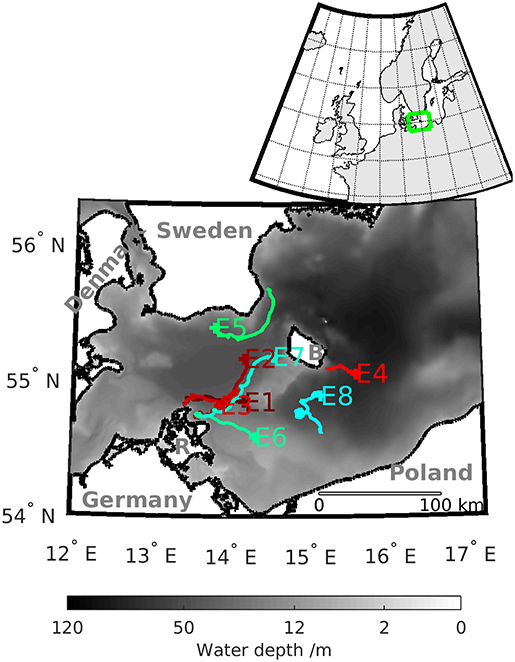
Figure 1. Bathymetry of the Western Baltic Sea and the numbered tracks of the selected eddies detected with M_V. The label of the tracks indicates the position where the eddy decays. The island of Rügen is marked with R and the island of Bornholm with B. The insert in the upper right corner shows the position of the Western Baltic Sea on the European shelf.

In general, the Baltic Sea is one of the largest brackish water bodies worldwide. It especially suffers from decade-long external and internal nutrient loading. Increased nutrient inputs, by, for example, nitrogen (N) and phosphorus (P), leads to recurring algal blooms. First, blooms occur during March, and collapse latest in the middle of April, due to N limitation. This N limitation lasts until summer in the Western and central Baltic Sea (HELCOM, 2017), due to low dissolved inorganic nitrogen concentrations (DIN) but dissolved inorganic P concentrations (DIP) are always detectable (Nausch M. et al., 2008). The ratio of DIN:DIP is low and decreases further during the summer (Nausch G. et al., 2008). These conditions support cyanobacteria blooms, that consist of for instance, Nostocophyceae (Wasmund et al., 2011), which are especially adapted to these environmental settings. Those blooms can be very persistent, due to the ability of the species to take up and store P fast, or to fixate N (e.g., Ritchie et al., 1997; Larsson et al., 2001; Aubriot et al., 2011). Therefore, in contrast to other phytoplankton groups, cyanobacteria blooms are not N-limited during summer. This feature is also represented in the model used here. Stigebrandt et al. (2014) stated that internal nutrient sources, i.e., nutrients emanating from anoxic waters, are even more important for the ecology of the Baltic Sea, than external sources, i.e., nutrient inputs from the land. Usually, nutrient depleted phytoplankton would stop growing and be consumed by zooplankton. This consumption would recycle some nutrients, but some will sink out of the euphotic zone. Therefore, phytoplankton would soon stop their growth. However, we assume that eddies can bypass phytoplankton's growth stagnation, by transporting nutrient-rich coastal upwelling water back into the open sea. These nutrients would be added to the internal sources from anoxic waters and, therefore, prolong the growth opportunities of phytoplankton. As a result, eddies can maintain optimum growth conditions for phytoplankton by providing horizontal nutrient transport (DIN and DIP) during summer. On the other hand, eddies can act as a niche for phytoplankton growth due to the different physico-chemical properties inside the eddy compared to the outside water masses. This difference is maintained for the whole lifetime of the eddies. In addition, this coherent nutrient transport could indirectly support plankton even in regions that are not directly connected to external (river) and internal (upwelling, anoxic waters) nutrient supplies. This leads to the hypothesis that eddies have a multifactorial impact on nutrient (transport) and plankton (niche) dynamics in the Baltic Sea and its coastal regions.

To check this hypothesis, we used data from a coupled hydrodynamical-chemical-biological model ERGOM (Ecological Regional Ocean Model) developed at the Leibniz Institute for Baltic Sea Research (www.ergom.net) for the Western Baltic Sea for a time interval from March to October 2010 to present a case study for selected eddies. We investigated the dynamics of a planktonic community consisting of small and large phytoplankton (flagellates resp. diatoms), zooplankton and cyanobacteria as well as dissolved nutrients like PO₄, NH₄, and NO₃ within selected eddies during their lifetime. The residence time of water masses inside the eddy plays a crucial role for the plankton dynamics. Therefore, we investigated the residence times inside our selected eddies and compared the dynamics of plankton and nutrients within the coherent water bodies for different eddies.

Please note, the aim of this paper is a qualitative description of the effects of eddies on the plankton community. All quantitative results are used only to estimate the order of the effects, because the quantitative results depend on the parametrization of the model.

The paper is organized as follows: First, we introduce the methods used to detect and track eddies (Vorticity based Lagrangian descriptor M_V) as well as those employed to quantify the amount of coherently transported plankton and nutrients (Transfer operator approach TOA and tracer analysis TA). Then, we present the studied data set. Subsequently, we will give an overview of our test case eddies. Finally, we discuss the effect of eddies on the dynamics of plankton concentrations within the eddy. General findings and open questions are discussed in the conclusions.

2. Materials and Methods

2.1. Tracking Eddies

In this section, we briefly present the methods applied to detect and track eddies (Vorticity based Lagrangian descriptor in section 2.1.1), to quantify the coherent core of the eddy (Transfer operator approach in section 2.1.2) and to calculate the residence time of water masses inside the eddy and the transported amount of nutrients and plankton (tracer analysis in section 2.1.3). Throughout the paper we refer to the Lagrangian descriptor-based eddy tracking as M_V, the transfer operator approach as TOA and the tracer analysis as TA.

2.1.1. Vorticity Based Lagrangian Descriptor M_V

The used eddy detection and tracking method is based on the approximation of Lagrangian coherent structures that separate the fluid flow into regions of qualitatively different dynamical behavior. The search for eddies relies on the concept of Lagrangian descriptors developed to identify certain points in the flow which can be linked to the eddy core and the boundaries of regions around these points which can be linked to the eddy shape. We refer to Mancho et al. (2013) for details on Lagrangian descriptors in general and to Vortmeyer-Kley et al. (2016) for details on M_V and the implementation of the specific eddy detection tool used in this study. Here, we will only provide a brief outline.

Firstly, the Lagrangian descriptor M_V has to be calculated for each point in space and provides a map of M_V at any given time instant. This quantity M_V is related to the vorticity, i.e., a measure of the strength of rotation a fluid particle experiences along its path for a finite time interval 2·τ (mathematical details cf. Vortmeyer-Kley et al., 2016 and Lünsmann et al., 2018). Fluid particles that stay in regions of strong rotation collect large values of this measure. This is the case inside the eddy or especially in the eddy core. Outside the eddy, the collected values of the measure are smaller, thus at the boundary between the eddy and the surrounding region, a sudden change in the measure M_V is visible. This sudden change can be linked to the eddy boundary.

Secondly, this map of M_V is calculated for each time step. The eddy's core and shape can be detected for each time step, and hence, the movement of each eddy as well as the changes in its shape can be tracked. The result is a track for each eddy as for example in Figure 1.

The parametrization of the eddy detection was chosen as follows:

The finite time interval 2·τ to calculate M_V was chosen to be 72 h to resolve long living as well as short living eddies. The search window for the detection of the eddy core was 4.8 km in radius and the search window for the eddy shape was chosen as 30 km to cover a broad range of eddies from submesoscale with eddies' radius smaller than the internal Rossby radius of deformation [≈ 5 km in the Baltic Sea (Fennel et al., 1991)] to mesoscale.

2.1.2. Transfer Operator Approach TOA

For the identification of the part of the eddy that does not mix with the surrounding flow, i.e., the coherently transported water mass, we employed a modified transfer operator approach (TOA).

While the Lagrangian descriptor M_V can detect eddies and estimates their size and lifetime computationally as cheap in large velocity fields, it is a non-objective method in the sense of Haller (2015) that is not able to infer coherently transported water masses from velocity data. Transfer operator approaches, however, constitute a class of objective Lagrangian methods that have been developed for the exact purpose of detecting weakly mixing subsets in stationary and non-stationary flows (Dellnitz et al., 2009; Froyland and Padberg, 2009; Froyland et al., 2010). Here, the eddies that we identify using M_V serve as an approximation and are further analyzed using TOA to extract the boundary of the coherent water masses.

The essential idea of the original transfer operator approach (e.g., Froyland and Padberg, 2009) is to divide the domain of interest into smaller parts, so-called tiles, and to approximate the complicated flow that carries and deforms the domain by a graph of transfer probabilities between these parts. The domain parts are then grouped such that the inter-group mass exchange is minimized.

The employed approach has been modified to meet the conditions of fast changing, turbulent currents close to the coastline with the goal to find water bodies that are coherent on biological time scales but are allowed to change on larger time scales. The approach is based on ideas discussed in Froyland and Padberg (2009), Froyland et al. (2015), and Lünsmann and Kantz (2018). Since the discussion of this novel method exceeds the scope of this paper, we refer to Lünsmann et al. (2018) for details. Here, we will only provide a summary.

In short, for each time step, we selected an area on the basis of the eddy shape and center provided by M_V. This domain is discretized into square tiles with edge length 0.002°, i.e., approx. 200 m (see Lünsmann et al., 2018 for details of the selection process).

Using this partitioning and an integration time of ±36 h, we computed the impact of transport into the future and past on the mixing of fluid volume by means of filamentation (see Figure 2A). The joint effects are described by a time-centralized transfer operator which is basically, a graph of transition probabilities between tiles (see Figure 2B).

FIGURE 2

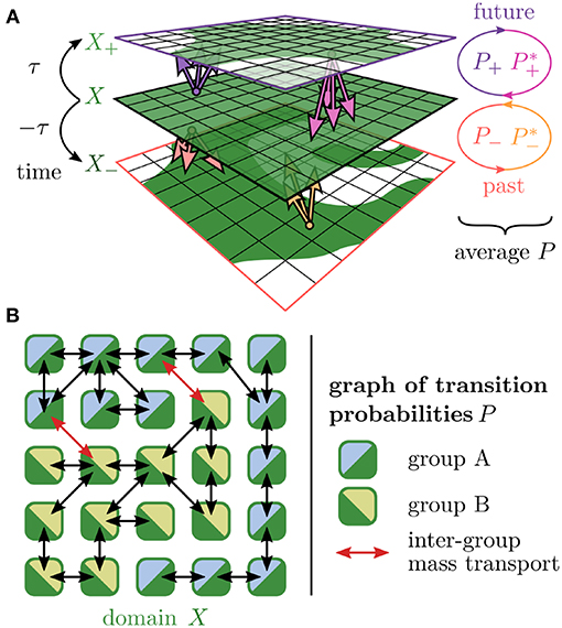
Figure 2. Original time-centralized transfer operator approach. (A) Domain X (green) is transported into future and past with an integration time of τ. The images X⁺ and X⁻ are used to compute matrices of transfer probabilities P₊ (into future, pink) and P₋ (into past, orange) between tiles. The combined effects of transport and reversed transport captured by these matrices and their time-reversed counterparts $P_{+}^{*}$ and $P_{-}^{*}$ yield a time-centralized transfer probability matrix P. (B) This matrix P depicts a graph of mass transport that is the basis of an analysis with the aim to separate the tiles X into two groups A (blue) and B (lime) such that the inter-group mass transport (red links) is minimized.

Subsequently, we merged the domain boundary to facilitate the separation of the inner coherent core and outer surrounding flow. The resulting modified time-centralized transfer operator was used to compute the affiliation of each tile with the inner coherent core. These affiliation values were arranged into an indicator vector. In addition, we computed transfer operators to couple adjacent time steps in both time directions. These transfer operators are then used to identify the size of the coherent mass as follows: Assuming that the mass of the coherent water body does not significantly change under time evolution, we created a threshold for the indicator vector of each time step such that the transport probability between adjacent time steps was maximized while also keeping the mass of the structure approximately constant at all times. The assumption was plausible for the analysis of two-dimensional flows and facilitated the search for accurate thresholds.

At several points during the analysis, it was possible to check whether the coherence of the inferred structure was plausible. Using these checks, we only investigated time intervals (later on referred to as coherence times) for which it was not apparent that the structure was significantly weakened or the mass of the coherent core drastically changed. This way, we minimized the impact of obstructive events, like eddy formation, eddy destruction and front collision, on our analysis.

The result of this procedure is a sequence of spatial partitions that estimate the evolution of the coherent eddy core. While mass exchange between the resulting structure and the ambient water was minimized, fluid transport across the boundary still occurred accounting for fluid loss, or entrainment of small filaments. We chose this approach because it provided maximal consistency over long periods while avoiding the formation of filaments.

2.1.3. Evaluation of Coherence: Tracer Analysis (TA)

To probe the impact of hydrodynamic structures on biological processes it is of great interest for how long water masses stay inside the eddy.

Since the obtained boundaries of an eddy are by design not completely impenetrable, especially for time periods longer than the observation horizon of τ = 36 h, we focused our analysis on the water mass that stays within those boundaries and thus stays truly coherent. For this purpose, we only considered points in the region of the inner eddy core that—when integrated backwards in time—stay inside the detected boundaries for at least 80% of the observed coherence time before first leaving the structure. This was a purely conservative precautionary measure.

For this computationally rather expensive tracer analysis (TA) we covered the estimated eddy cores with tracers and integrated their backward and forward trajectories numerically. This was done using Heun's method with an integration time of $\Delta t=\frac{1}{8}$ h while the given velocity fields were interpolated linearly in space and time.

Figure 3 illustrates the differences between the shapes detected with M_V and TOA and shows the region detected by TA based on the results of TOA. M_V gives an estimate of the shape of an eddy, TOA defines the coherent set for each time step and TA yields the area fraction of TOA with a common history.

FIGURE 3

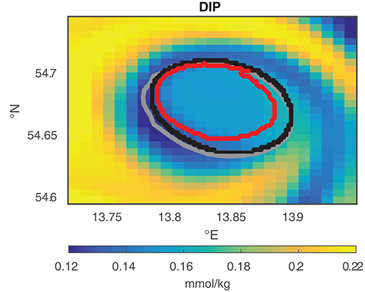
Figure 3. Comparison of the eddy shapes of M_V (gray), TOA (black), and the TA area fraction that stays 80% of the actual age of an eddy together (red) for eddy E2 at April 11, 2010 09:00 a.m. The color-coded map shows the dissolved inorganic phosphorus (DIP) concentration inside and around the eddy at this instant of time, with low concentration inside the eddy shapes and higher concentrations around the eddy.

2.1.4. Reference Water Body

TOA and TA were used to describe the dynamics of selected eddies, especially their shape and their coherence time. For the description of the plankton dynamics inside and outside the eddy we defined the inside as the area enclosed by the eddy boundary as detected by TOA, respectively, TA and the outside as an area around the eddy. We chose the longitudinal (x) and latitudinal (y) extents of the area outside the eddy, twice as large as the extents of the inferred eddy core (see Figure 4). The reason to couple the area outside the eddy to the area inside the eddy was to compare the dynamics in similar area fractions for the eddy at different instants of time.

FIGURE 4

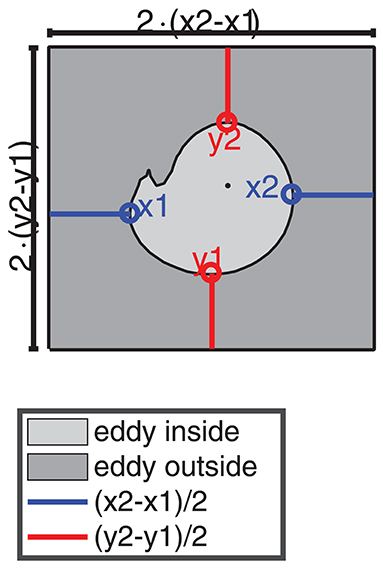
Figure 4. Schematic sketch how the area inside and outside of an eddy is chosen. The light gray area indicates the region inside the eddy (here an eddy with a small filament). The dark gray box around the eddy is the area outside the eddy. The blue and red lines indicate the distance of the outer edges of the eddy boundary in x and y direction x1, x2, y1, and y2 to the box boundaries. The black dot indicates the eddy center.

2.2. Setup of the Hydrodynamical-Biogeochemical Model of the Western Baltic Sea

In order to generate the velocity fields to conduct the eddy tracking, we rely on the output of a numerical model of the Western Baltic Sea. The model settings are similar to Gräwe et al. (2015) and Vortmeyer-Kley et al. (2016). Figure 1 shows the area of study. The insert in the left upper corner indicates the location of the Western Baltic Sea on the northern European Shelf.

The hydrodynamic model core is the state-of-the-art coastal ocean model GETM (General Estuarine Transport Model) (Klingbeil and Burchard, 2013; Klingbeil et al., 2018). The horizontal resolution of the model is 1/3 nautical miles, which is approximately 600 m. We applied 50 vertically terrain-following layers with adaptation toward stratification and a maximum surface layer thickness of 50 cm. Lateral diffusion of momentum, salinity and temperature along these model layers was carried out with a harmonic Smagorinsky diffusivity and a turbulent Prandtl number of three. Vertical diffusivities were obtained from GOTM (General Ocean Turbulence Model; Umlauf and Burchard, 2005), here based on a k−ε model with an algebraic second-moment closure. The second-order Superbee scheme with reduced numerical mixing (Klingbeil et al., 2014) was chosen for the advection of all prognostic quantities (including k, ε, and all biogeochemical state variables).

The ocean model is coupled with ERGOM (Ecological Regional Ocean Model) developed at Leibniz Institute for Baltic Sea Research (www.ergom.net). The biogeochemical module ERGOM consists of three dissolved inorganic nutrients (nitrate, ammonium, and phosphate), three functional phytoplankton groups (large and small cells, cyanobacteria (nitrogen fixers)), fast-sinking dead organic material and a bulk zooplankton which grazes on phytoplankton. Detritus is partly mineralized back into ammonium and phosphate while the other portion accumulates at the sea bottom where it is subsequently buried, mineralized or resuspended. All state variables were linked via advection-diffusion equations to the circulation model. Using stoichiometric ratios, the production and consumption of oxygen was calculated from all biogeochemical processes. Vice versa, the oxygen conditions determined whether phosphate was bound to iron in the sediment (oxic situation) or was released (during anoxia). The basic equations and assumptions as well as some validation are given by Neumann (2000), Radtke et al. (2012), and Schiele et al. (2015).

The concentrations of the plankton species are given in mol of carbon per kg of water and are thus a measure of biomass. Changes in concentration refers therefore to biomass and not to cell count.

To account for riverine nutrient loads, we linearly interpolated the 2-weekly measured nutrient concentrations to daily values. The riverine freshwater discharge was measured on a daily basis and directly provided to the model. Contribution of atmospheric deposition of nitrogen (N) and phosphorus (P) was marginal as it constituted less than 2% (N) and 0.5% (P) to overall loads. The atmospheric deposition was provided as a spatially uniform and constant climatological value.

The atmospheric forcing was derived from the operational model of the National German Weather Service with a spatial resolution of 7 km and temporal resolution of 3 h.

The entire model output (physics and biogeochemistry) was converted from terrain-following coordinates to equidistant geopotential z-levels with a vertical grid spacing of 1 m in a post processing. Afterwards, we averaged the model output over the upper 10 m of the water column. The model output covers the time between March 2010 and October 2010, which is the plankton growth season, with a temporal resolution of 1 h and was taken out of a multidecadal simulation.

3. Results and Discussion

3.1. Eddies in the Western Baltic Sea

The data set provided by the coupled chemical-biological and hydrodynamic model contains velocity fields as well as temperature, salinity, zooplankton, cyanobacteria, small, and large phytoplankton concentration fields as well as concentration fields for NO₃, NH₄, and PO₄ for the period from March 1 to October 31, 2010.

Using the eddy tracking tool based on the Lagrangian descriptor M_V we found 28 391 eddies that live longer than 2 h within this time interval. Reißmann (2005) detected between 0.025 and 0.1/km³ eddies per volume within the density data field in his CTD measurement campaign in the Arkona Basin and Bornholm Basin. If we compare our number of eddies to the volume of the Western Baltic Sea, we find 13/km³ eddies per volume. However, the results by Reißmann (2005) are based on measurement campaigns within a limited time period per basin on a 5 km grid that covers only the deeper parts of the basins. His eddy definition is based on the detection of isolated anomalies in pressure. Karimova and Gade (2016) detected around 7000 sub-mesoscale eddies in the entire Baltic Sea based on SAR images between 2009 and 2010. However, even these Karimova and Gade (2016) cannot directly be compared to ours. They defined eddies by their signature in the SAR images and not based on structures in the velocity field that cannot be crossed by trajectories. Furthermore, SAR based eddy detection suffers from cloudiness and lower spatial resolution. Nevertheless, most of our eddies exist only for short time intervals. Only about 2% of the eddies live longer than 100 h, i.e., in time intervals that are comparable to biological time scales (Lehtimaki et al., 1997; Wasmund et al., 2012). Long-living eddies arise in the deeper parts of the Western Baltic Sea. Looking at the propagation distance, about 10% of the eddies travel longer than 8 km, here the propagation distance is defined as the Euclidean distance between the start and the endpoint of the eddy track neglecting all meandering with the flow. Some single eddies even travel up to 60 km and thus can potentially contribute to transport over long distances. The combined criterion of lifetimes longer than 100 h and travel distances larger than 8 km is fulfilled only by 1.5% of all detected eddies.

For our analysis, we selected eight eddies from different regions of the Western Baltic Sea with a focus around the island of Rügen where most eddies arise (see Table 1). Their times of emergence covered the different blooming preferences of the species during the growth season. Therefore, they can serve as examples of eddies' possible impact on blooming behavior. Wasmund et al. (1998) noted, depending on the water temperature, that diatoms (lpp) would usually bloom in March (high nutrients, low temperature), whereas dinoflagellates (spp) would follow in April (lower nutrients, higher temperature). Cyanobacteria would usually occur during summer, followed by diatom blooms in autumn (Wasmund et al., 2011). Thus, each selected eddy represents one month of the planktonic growth season.

TABLE 1

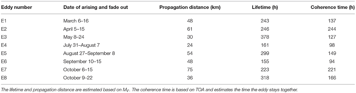
Table 1. Selected eddies in the Western Baltic Sea between March 1, 2010 and October 31, 2010 detected with the eddy tracking tool based on M_V.

All selected eddies were cyclonic eddies and rotate counterclockwise because anticyclonic eddies in our study area showed only short coherence times and therefore did not fit into our study. Some of the selected eddies arose from upwelling events along the Polish coast, the coast of Bornholm and the coast of Sweden. Thus, they can serve as examples for the coastal export of nutrients and plankton.

An overview of the tracks of the selected eddies can be found in Figure 1. Eddies' lifetime and propagation distance based on the estimate of M_V are presented in Table 1. Furthermore, Table 1 lists the coherence times of the eddy, i.e., the time an eddy stays coherent, based on TOA.

3.2. Residence Times of Water Masses Inside Selected Eddies

In order to gain insights into the impact of eddies on biological growth processes, the lifetime of eddies and the biological time scales should match in the sense that the eddy lives significantly longer than the doubling time of the plankton species. The lifetimes of the chosen testcase eddies were about 3- to 8-fold of the plankton doubling time of the slowest growing plankton group (cyanobacteria with a maximum growth rate of 0.5/day) contained in the biogeochemical model, neglecting nutrient limitation and predation. Predation limits the growth depending on the supply of prey with a maximum grazing of 0.5/day. However, all growth rates were light and/or temperature dependent. Thus, effective growth was in general lower.

In order to determine whether water was really trapped inside the eddy, we investigated the residence time of water masses inside the eddy shapes detected with TOA applying the tracer analysis (see section 2.1.3). During this time, the exchange between the eddy and the surrounding water was minimized. Furthermore, we studied the area fraction of the eddy that remained coherent.

Figure 5 shows the eddies' shapes at the first detection of the coherent eddy (A), at half of the coherence time of the eddy (B) and at the last detection of the coherent eddy (C) for all selected eddies based on the quantification with TOA. The color-code shows the residence time of the tracers inside the eddy in relation to the eddy coherence time.

FIGURE 5

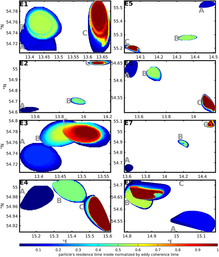
Figure 5. Color-coded residence time of tracers in relation to the eddy coherence time inside the selected test case eddy shapes at (A) the first detection of the coherent eddy, (B) half of the coherence time of the eddy and (C) the last detection of the coherent eddy. The shapes are based on TOA and the residence times on TA.

This way Figure 5 illustrates the aging of the eddy. In the last stage (C) most of the eddies in Figure 5 showed a large region of tracers with residence times close to the eddy coherence time. Regions with lower residence times can be found at the boundaries of the eddy shape and point at small scale exchange processes. Overall, 63–98% of the area of the first detection of the coherent eddy stay 80% and more of the coherence time inside the eddy. This is a rather large percentage, if we compare it to a transfer operator-based study of the Agulhas rings by Froyland et al. (2015) that finds 80 to 85% of the enclosed water stay inside the eddy during its lifetime of 2 years. Note, that the Agulhas rings are stable, large, far-traveling and long living structures in contrast to the small and short living eddies in a turbulent environment considered here.

Assuming that eddies have a vertical extend of 10 m, between 0.18 km³ up to 0.51 km³ water is transported by the eddy during its coherence time. Reißmann (2005) stated, based on CTD measurement campaigns, that 12% of the total volume of their analyzed data fields in the Western and the central Baltic Sea was occupied by eddies independently of the season. For the Western Baltic Sea this corresponds to an occupied volume of about 255 km³. Assuming that about 1.5% of all eddies in the blooming season (about 450 eddies) are relevant with respect to lifetime and propagation distance and have a mean volume of about 0.3 km³, then about 135 km³ of water is transported. This amounts to approximately half of the occupied volume.

Furthermore, we found eddy cores that remained coherent over nearly the whole eddy's lifetime. Comparing their coherence times with the plankton doubling times, the coherence times were 2- to 5-fold of the plankton doubling time of the slowest growing prey group (cyanobacteria) contained in the biogeochemical model, neglecting nutrient limitation and predation. This coherence time is low compared to the study of d'Ovidio et al. (2010) where eddies possibly formed niches for up to several months in the southern Atlantic. However, when comparing coherence times and the time scales of plankton bloom formation in the Baltic Sea, we can conclude that though the coherence times are smaller than the lifetimes of eddies they are still in the same order of magnitude as the biological time scales (Lehtimaki et al., 1997; Wasmund et al., 2012). Hence, an impact of eddies on biological processes can be expected.

3.3. Case Study of Selected Eddies' Impact on Plankton Growth and Distribution

We calculated the mean concentration of dissolved nutrients (DIN=NO₃+NH₄, DIP=PO₄) as well as of plankton (small phytoplankton (spp), large phytoplankton (lpp), cyanobacteria (cya), and zooplankton (zoo)) inside the area fraction described by TA that shares a common history for each instant of time. The tracers that make up this area fraction stay at least 80% of the actual age of an eddy inside this area. Thus, the plankton community and the nutrient pool they are feeding on is almost not disturbed from outside. Those concentration values were compared with concentrations in a reference water body outside the coherent part of an eddy that was chosen as described in section 2.1.4.

We expected two different behaviors of eddies depending on their time of occurrence during the year:

(a) Eddies with transporter properties: they transported an enclosed water body including nutrients and plankton community. The nutrient and plankton concentrations inside the eddy showed no or only minor changes during the transport. Thereby, concentrations of plankton and nutrients can differ between inside and outside the eddy before the eddy fades out or loses coherence.

Eddies with transport properties of dissolved inorganic nutrients and plankton were expected to arise in spring after the early spring bloom. The nutrient depletion after spring bloom (Nausch M. et al., 2008; Schneider et al., 2017) and the low temperatures hinder plankton growth inside the eddy and an enclosed nutrient budget could be transported, for example, from the coast into nutrient depleted regions in the open sea.

(b) Eddies with niche properties: here the enclosed water body acts as a fluid dynamical niche. A fluid dynamical niche provides competitive advantages for one/several functional groups (d'Ovidio et al., 2010) due to various factors such as different temperature/salinity, higher nutrient concentrations, another nutrient composition, the absence of predators or the presence of prey for the predators, compared to the ambient water. The dynamics inside the eddy is characterized by a rapid decrease of nutrients inside the eddy and a temporal increase of plankton concentrations driven by nutrient supply, followed by a decrease caused by nutrient limitation inside the eddy.

We expected that eddies within summer and autumn months tended to show niche properties, because higher temperatures and trapped nutrients drive the plankton growth (Neumann, 2000).

We tested these two hypotheses for the selected eddies representing each month of the growth season, by comparing nutrient and plankton dynamics inside and outside the eddies. Additionally, we checked temperature and salinity to characterize the physical conditions for plankton growth. Here, nutrients were treated as dissolved inorganic phosphorus (DIP=PO₄) and dissolved inorganic nitrogen (DIN=NH₄+NO₃). Note, that all concentrations were obtained from model calculations and yielded partly very small values, which would be below the detection limit in measurements. These values are ignored in the discussion.

It is important to note that all eddies can have a combined effect on the ecosystem with a tendency to have more transporter or more niche properties for one or several quantities (nutrient or plankton). The following case study is based on the dominant property of each eddy.

3.3.1. Transport of an Enclosed Water Body

Eddies E1-E4 acts more as transporters. Figure 6 gives an overview of the dynamics of the temperature inside and outside the eddy as well as the dynamics of the concentrations of nutrients and plankton during the coherence time of the eddy. Note, that the lifetime of the eddy indicated by the eddy track can be longer than the coherence time. The dynamics are only shown for the coherence time of the eddy. The results of the dynamics are based on an area fraction described by TA that shares a common history. The tracers that make up this area fraction stays for at least 80% of the actual age of an eddy inside this area. The concentration time series of nutrients and plankton inside and outside the eddy are smoothed with a 5 h-moving mean to avoid temporal fluctuations that could be misinterpreted as increase or decrease.

FIGURE 6

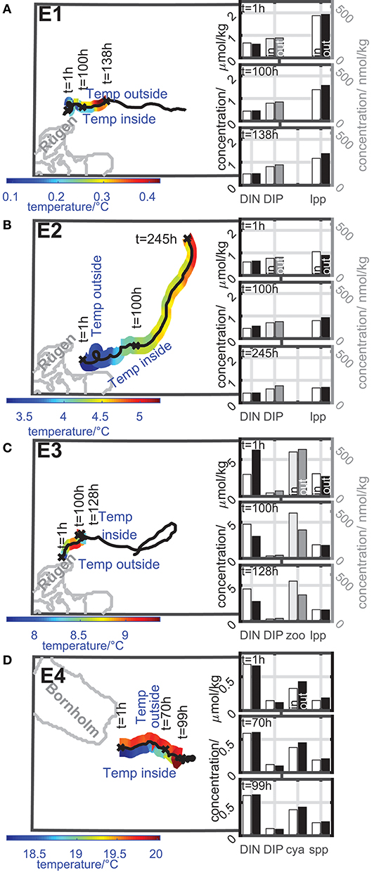
Figure 6. Color-coded dynamics of the temperature inside and outside the eddy along the eddy track during its coherence time of eddies with transporter properties ((A) E1, (B) E2, (C) E3, and (D) E4). Insert bar plots: concentration of nutrients and selected plankton groups inside and outside the eddy at selected timesteps of the concentration time series. Left concentration axis: black and white bars; right concentration axis: gray scaled bars. Dynamics inside the eddy: white and light gray bars; dynamics outside the eddy: black and dark gray bars. Further details see text.

For all eddies, the temperature (see Figure 6) and nutrient composition deviated from the ambient water as expected for a coherent water mass. The eddies E1-E3 arose along the coast of Rügen, E4 arose along the coast of Bornholm. In all cases coastal water was trapped by the eddy and transported into the open Baltic Sea.

Eddy E1 and E2 show a similar behavior (Figures 6A,B). They both arose in early spring close to Rügen when the water temperature is low and nutrient concentrations are still high to form a first spring bloom. Nutrient concentrations and large phytoplankton concentration inside the eddy do not change much during the coherence time. Small phytoplankton, cyanobacteria, and zooplankton concentration are very low. The temperature inside the eddy is lower than outside in all cases and limits the planktonic growth. An exception was eddy E2 after t = 100 h where the eddy entrains a warm filament which led to an increase of temperature of about 0.5°C inside the eddy. This entrainment can be observed in the hourly evolution of the modeled temperature field and the TOA eddy shape (not shown here). Due to the definition of coherence for a finite time interval and the idea of TOA to preserve a constant volume during this coherence time, the interaction with the warm filament becomes part of the eddy's history and increases the temperature inside. After this, the eddy transports warmer water than the ambient water until it fades out.

Eddy E3 arose in the late spring when the water temperature is higher and nutrient levels are lower after the spring bloom (Figure 6C). This eddy exports a bloom of large phytoplankton from the coast to offshore. The large phytoplankton concentration is higher in the first detection of the coherent eddy and decreased during the coherence time due to limited nutrient supply, natural mortality, and grazing. The zooplankton concentration showed a small increase due to a prey supply in form of large phytoplankton and decreased afterwards. The cyanobacteria and the small phytoplankton concentration are still very low.

Eddies E1 to E3 showed a trend of decreasing shares of large phytoplankton, in accordance with long-term monitoring for this area (Wasmund et al., 2011).

Eddy E4 arose in summer from a small-scale upwelling event of cold water at the coast of the island of Bornholm (Figure 6D). The nutrient concentrations were low both inside and outside the eddy and did not change much during the coherence time of the eddy. At the time, the small phytoplankton and the cyanobacteria biomass concentration were in a detectable range and showed a very small increase by about 0.1μmol/kg driven by the temperature increase of about 1.5°C. However, due to the nutrient limitation in summer, the nutrient concentrations as well as the plankton concentrations were in general low inside and outside the eddy. Interestingly, the large phytoplankton concentration was of the same order of magnitude as the cyanobacteria concentration and showed a similar behavior as the cyanobacteria inside the eddy. The large phytoplankton growth was not driven by the temperature because the growth was modeled as temperature independent. The reason for an increase could be nutrient supply or a decrease in grazing pressure. Wasmund et al. (2011) described a lower larger phytoplankton biomass for this area and time of the year, than during spring. In fact, large phytoplankton of E4 (Bornholm) has the same biomass in summer as large phytoplankton of E1-E3 (Rügen) in spring. It is therefore difficult to compare phytoplankton developments with different origins, even on a comparably small geographical scale like the Baltic Sea. The large phytoplankton concentration outside E4 followed the concentration development inside. The zooplankton concentration was one order of magnitude smaller than the phytoplankton concentrations and showed slightly lower, minimally increasing values inside the eddy E4 compared to outside.

To gain more insights into the transport properties of eddies in the Baltic Sea, we now provide some rough estimates of the total transport of nutrients.

Based on the findings in Figure 5 we can estimate the lower boundary of the transported volume. We estimated the area of the first detection of the coherent eddy that stayed 80% and more of the coherence time inside the eddy and assumed a vertical extend of 10 m for each eddy. The resulting volumes are presented in Table 2. To give a rough estimate of the possible transported amount of nutrients in the Baltic Sea we used measurement data for NO₃, NH₄, and PO₄ in the water column from the monitoring research cruises (Terminfahrt 2010/03, /05, and /07) by the Leibniz Institute for Baltic Sea Research Warnemünde, Germany in the Arkona and Bornholm Basin 2010. The data set contains ammonium, nitrate and phosphate measurements in the water column in different depth at different positions. Each cruise takes water samples in approximately the same region. From these data we calculated mean DIP and DIN in the upper 10 m of the water column in those regions where the eddies arise and travel. These mean values and the eddy volume can be used to estimate how much nutrients could be contained in the eddy volume (see Table 2).

TABLE 2

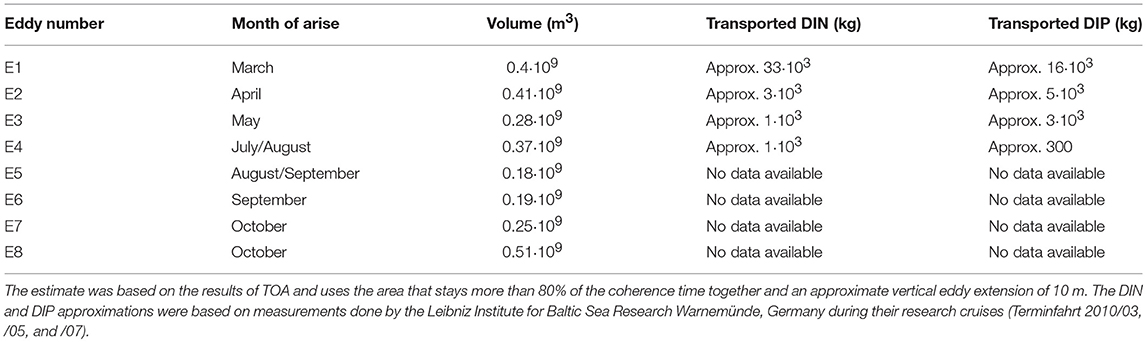
Table 2. Transported volume and amount of DIN and DIP of eddies with transporter properties.

Interestingly, the eddies E1–E3 from the German coast transported in total about 25 000 kg of DIP from the coast into the Baltic proper. This amount is almost 1/4 of the German aim to reduce the export of total phosphorus into the Baltic Proper (HELCOM, 2013). A large amount of DIP probably came from upwelling waters. However, it is reasonable to assume that non-point run-off from coastal zones will be transported as well. This diffuse non-point run-off is already included into the model with estimations from state monitoring (see section 2.2). The amount of transported DIN is low (about 38 000 kg), compared to the amount of necessary reductions of 7·10⁶ kg total nitrogen exported from Germany. Therefore, the impact of such eddies is higher on modeled cyanobacteria blooms within the Baltic Proper, as they rely more on P than N (Neumann, 2000). Furthermore, only four of all possible eddies from the Western Baltic Sea zone were included in this calculation. However, 1.5% of all eddies, i.e., in sum 450 eddies, live long enough and travel far enough to be relevant for transport or as niche. Thus, the amount of transported nutrients is probably higher.

3.3.2. Fluid Dynamical Niche

The eddies E5-E8 are examples of eddies which tend to niche properties. Figure 7 gives an overview of the dynamics of the temperature inside and outside the eddy as well as the dynamics of the concentrations of nutrients and plankton during the coherence time of the eddy E5, E6, E7, and E8 as described in general for Figure 6 for the eddies E1-E4 in section 3.3.1.

FIGURE 7

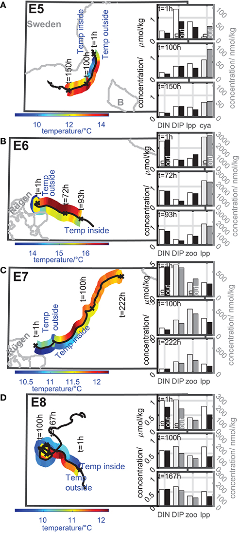
Figure 7. Color-coded dynamics of the temperature inside and outside the eddy along the eddy track during its coherence time of eddies with niche properties ((A) E5, (B) E6, (C) E7, and (D) E8). Insert bar plots: concentration of nutrients and selected plankton groups inside and outside the eddy at selected timesteps of the concentration time series. Left concentration axis: black and white bars; right concentration axis: gray scaled bars. Dynamics inside the eddy: white and light gray bars; dynamics outside the eddy: black and dark gray bars. Further details see text.

The eddies arise in late summer and autumn in different regions. Eddy E5, E7, and E8 arise from small scale or large-scale upwelling events.

Eddy E5 arises in late summer from an upwelling at the coast of Sweden (Figure 7A). Therefore, the temperature inside the eddy is much lower than outside. The nutrient concentrations inside the eddy especially DIP decreases during the coherence time and the cyanobacteria concentration inside increases. The large phytoplankton concentration inside the eddy is more or less constant during the first 100 h of the eddy's lifetime and decreases slightly afterwards. This behavior can be linked to the ability of the eddy to trap nutrients, which can be consumed by the cyanobacteria leading to an increase in cyanobacteria's biomass. The decrease of the large phytoplankton is caused by the limited supply of DIN. A higher DIN concentration could lead to further growth of large phytoplankton inside the eddy. The growth of the cyanobacteria is not limited by DIN because its growth is only DIP dependent in the model (Neumann, 2000). The zooplankton and the small phytoplankton concentrations are much smaller and show minor biomass increases by up to 20 nmol/kg.

Eddy E6 arises in early autumn close to Rügen (Figure 7B). The nutrient concentration, especially DIN, inside the eddy decreases by around 30–40% during the coherence time. Simultaneously, the large phytoplankton decreases slightly by about 0.5 μmol/kg, while the zooplankton biomass concentration inside the eddy increases by about 0.2 μmol/kg. In this sense the eddy provides a niche in terms of nutrients and prey by providing nutrients for large phytoplankton, which is able to reproduce itself about 4-times within the eddy's coherence time. Subsequently this growing phytoplankton population serves as a prey for the zooplankton. A similar effect can be observed for eddy E7 (Figure 7C). This eddy arises from a small scale upwelling close to Rügen in autumn. Therefore, we find a lower temperature inside the eddy compared to the ambient water. Here the DIN concentration inside the eddy decreases to about 1/4 of the starting concentration (about 1/2 for DIP). It would have been expected that phytoplankton would increase. However, large phytoplankton is nearly halved, although the coherence time is approximately 9-times the large phytoplankton doubling time. By contrast, the zooplankton biomass nearly doubles inside the eddy although the coherence time is only about 4-times the zooplankton doubling time. The zooplankton grazing consumes apparently almost the complete production of large phytoplankton. Such a result can be ecologically relevant, as fresh biomass can increase the reproduction success of zooplankton (Sanders et al., 1996). This finding means, that zooplankton proportions for this area might be different in the following years.

The eddy E8 arises from a large scale, long-lasting upwelling event in autumn at the Polish coast (Figure 7D). This event builds up a cold water front that decays into several eddies with temperatures of 1–2°C below the water temperature of the ambient water. DIP inside the eddy E8 decreases slightly by about 20% during the coherence time, while DIN shows a decrease by about 40%. The large phytoplankton inside shows a decrease by about 25%. The zooplankton shows nearly no decrease of biomass concentration. In comparison with the surrounding water masses the plankton concentrations are higher inside the eddy than outside. In this sense the enclosed nutrients from the upwelling event inside the eddy buffer the decrease of plankton and enable higher plankton concentrations inside than outside the eddy. The eddy provides better growing conditions than the surrounding water masses. Nevertheless, in autumn the growth is limited by the availability of light. This growth limitation at the end of the growth season leads to the fact that E8 can also be interpreted as transporter of zooplankton, because zooplankton does not show significant dynamics during the coherence time.

Furthermore, Berthold et al. (2018a,b) discuss the effect of nutrient availability on the plankton community in coastal waters in the Southern Baltic Sea. High precipitation can lead to an additional nutrient input from land runoff that increases plankton growth and enables a specific phytoplankton species composition in the coastal waters. Whether eddies that arise in these coastal waters and travel into the open sea like eddy E6 and E7 provide a fluid dynamical niche for this specific community is still an open question because the biogeochemical model considers only functional groups of plankton and not single species.

3.4. Open Questions of the Case Study

The presented study is based on a two-dimensional velocity field and a respective eddy detection. There are several open questions which would need a three-dimensional approach. In the following section we will address these open questions and limitations of our study.

One open problem linked to this missing three-dimensional biogeochemical-hydrodynamical model is, that we cannot estimate if there is up- or downwelling inside the eddy. However, up- and downwelling inside the eddy will also strongly influence the nutrient supply and subsequently enhance or suppress plankton growth as discussed in Martin (2003), Bakun (2006), and Gaube et al. (2014).

Another interesting open question is to what extent eddies interact with the nutricline. The impact of eddies on the thermocline has been discussed by McGillicuddy (2016) and a similar impact is possible on the nutricline. After the spring bloom the nutricline is lower in the Baltic Sea than before the spring bloom (Vahtera et al., 2007; Schneider et al., 2017). Eddies interacting with the nutricline and pumping nutrients upward can generate a short cut to biomass production.

Looking at the biogeochemical model several extensions are possible which perhaps change the interplay between eddies, plankton growth and community composition. Van Mooy et al. (2009) discuss the ability of phytoplankton to replace P under P-limited conditions. This might extend the growth of phytoplankton inside an eddy if P is depleted.

Furthermore, the model describes only functional groups and does not distinguish between different species with different properties. This missing consideration can have large consequences for the models' predictive power, as grazing can lead to a community shift. Although, the coherence times of the eddies considered are long enough to lead even to changes in the dominance of certain species as shown by Bastine and Feudel (2010) or Perruche et al. (2011) in theoretical studies, no such dominance changes in the Baltic Sea eddies have been observed. This could be either explained by the fact that the differences in the physico-chemical conditions inside and outside the eddies are too small. Moreover, the functional groups considered in Neumann (2000) comprise many species in each such group and represent thus only average behavior, while dominance changes are more probable to occur on a species level within one group, for example, in the group of diatoms. Even grazing preferences for specific species could change the dominance on the species level as discussed in Chakraborty et al. (2012) and Chakraborty and Feudel (2014) for a non-toxic-phytoplankton—toxic-phytoplankton—zooplankton—model. Additionally, there are trait-mediated feedback mechanisms described by Tirok et al. (2011), which might have to be implemented within the next years.

4. Conclusion

We have studied the impact of eddies on plankton growth to show that eddies can exhibit transport properties transporting plankton and nutrients and that they can provide a distinct niche with specific environmental conditions which are different from the ones in the ambient water. We have illustrated this behavior by studying effects of eddies on plankton and nutrient dynamics in the Western Baltic Sea in the blooming period from March to October 2010 in the form of a case study with selected eddies representing each month of the planktonic growth season.

The case study has shown that the selected test case eddies have a coherent core that stays together during large parts of the eddy's life time. From the TOA and TA study we can conclude that the largest parts of the waterbodies inside the eddy are most of the time (at least 80% of the coherence time) separated from the surrounding water. Hence, processes inside the eddy are to a large extent decoupled from processes outside the eddy. This coherence time of the eddy is of the order of several plankton doubling times. The dynamics of nutrients and plankton inside the coherent part of the eddy give rise to the fact that eddies can act in different ways. On the one hand, eddies E1-E4 can act as transporters trapping nutrient and plankton rich water and transporting it across larger distances. On the other hand, eddies E5-E8 can provide optimal growth conditions for either plankton itself or plankton as prey for zooplankton by trapping nutrients. This multifactorial impact shows that eddies in general do not act as a pure transporter or a pure niche, but have a combined effect on the ecosystem with a strong tendency either to be more a transporter or to act more as a fluid dynamical niche for one or several quantities (e.g., nutrient or plankton). An example is eddy E8 which has niche properties for nutrients and large phytoplankton as well as transporter properties for zooplankton.

The estimated transported volume and the corresponding transported amount of nutrients show that the role of eddies cannot be neglected in the export from the coastal region into the open sea. We estimated a volume transport of about 0.18 km³ up to 0.51 km³ water by a single eddy during its coherence time. Furthermore, we have shown that eddy-related transport of nutrients into the open Baltic Sea seems to be more relevant for DIP than for DIN. To gain more insights it is necessary to properly resolve the three-dimensional structure of an eddy, instead of assuming an extension of the surface eddy structure up to a depth of 10 m. To tackle this problem and others addressed in section 3.4 three-dimensional biogeochemical-hydrodynamical modeling of the Western Baltic Sea is needed as well as three-dimensional eddy tracking. The used methods M_V and TOA have the ability to be applied to three-dimensional velocity fields in a modified version.

Overall, the amount of long living and far traveling eddies is small in the Western Baltic Sea. If all eddies of this type could be checked automatically for their transported volume, one would be able to estimate the total transported amount of nutrients from the coast to the open sea. This could contribute to an explanation of the still high nutrient concentrations in the open Baltic sea. The share of eddy-transported nutrients compared to internal loading by anoxic water, or point sources is still an open question.

In summary, eddies can affect plankton growth and nutrient distribution in several ways enhancing or suppressing growth. To validate the postulated effects of eddies on plankton communities, measurements of plankton growth in eddies are necessary. Moreover, the study presented here considers only a two-dimensional velocity field averaged over the first 10 m in depth. A three-dimensional description and tracking of eddies can provide answers to the vertical transport of nutrients and prove the impact of concepts like upwelling or downwelling inside the eddy.

Data Availability

The datasets generated for this study are available on request to the corresponding author.

Author Contributions

RV-K did the eddy tracking based on M_V, selected the test case eddies and analyzed the concentration dynamics inside the eddies. BL developed and implemented the modified TOA to quantify the coherent core of an eddy and performed the tracer analysis. MB contributed the ecological interpretation of the concentration dynamics inside and outside the eddies. UG supervised the oceanic questions of this work and provided the velocity and concentration fields for the western Baltic Sea. The overall supervision was done by UF. All authors contributed to writing this manuscript.

Funding

RV-K would like to thank Studienstiftung des dt. Volkes for a doctoral fellowship and BMBF-HyMeSimm FKZ 03F0747C for funding. The publication of this article was funded by the Open Access Fund of the Leibniz Association.

Conflict of Interest Statement

The authors declare that the research was conducted in the absence of any commercial or financial relationships that could be construed as a potential conflict of interest.

Acknowledgments

We are grateful to the Norddeutsche Verbund für Hoch- und Höchstleistungsrechnen (HLRN) for access to their high-performance computing center, the analyzed model data was computed on the HLRN. Most parts of the eddy tracking were performed at the HPC Cluster CARL, located at the University of Oldenburg (Germany) and funded by the DFG through its Major Research Instrumentation Programme (INST 184/157-1 FUGG) and the Ministry of Science and Culture (MWK) of the Lower Saxony State.

The authors would like to thank Holger Kantz, Kathrin Padberg-Gehle, Tamás Tél, Anja Eggert and Peter Holtermann for stimulating discussions.

This research was performed within the scope of the Leibniz ScienceCampus Phosphorus Research Rostock.

References

Abraham, E. R. (1998). The generation of plankton patchiness by turbulent stirring. Nature 391, 577–580.

Google Scholar

Aguiar, A. C. B., Peliz, Á., and Carton, X. (2013). A census of Meddies in a long-term high-resolution simulation. Prog. Oceanogr. 116, 80–94. doi: 10.1016/j.pocean.2013.06.016

CrossRef Full Text | Google Scholar

Aubriot, L., Bonilla, S., and Falkner, G. (2011). Adaptive phosphate uptake behaviour of phytoplankton to environmental phosphate fluctuations. FEMS Microbiol. Ecol. 77, 1–16. doi: 10.1111/j.1574-6941.2011.01078.x

PubMed Abstract | CrossRef Full Text | Google Scholar

Bakun, A. (2006). Fronts and eddies as key structures in the habitat of marine fish larvae: opportunity, adaptive response and competitive advantage. Sci. Mar. 70, 105–122. doi: 10.3989/scimar.2006.70s2105

CrossRef Full Text | Google Scholar

Bastine, D., and Feudel, U. (2010). Inhomogeneous dominance patterns of competing phytoplankton groups in the wake of an island. Nonlinear Process. Geophys. 17, 715–731. doi: 10.5194/npg-17-715-2010

CrossRef Full Text | Google Scholar

Berthold, M., Karsten, U., von Weber, M., Bachor, A., and Schumann, R. (2018a). Phytoplankton can bypass nutrient reductions in eutrophic coastal water bodies. Ambio 47, 146–158. doi: 10.1007/s13280-017-0980-0

PubMed Abstract | CrossRef Full Text | Google Scholar

Berthold, M., Karstens, S., Buczko, U., and Schumann, R. (2018b). Potential export of soluble reactive phosphorus from a coastal wetland in a cold-temperate lagoon system: buffer capacities of macrophytes and impact on phytoplankton. Sci. Tot. Environ. 616–617, 46–54. doi: 10.1016/j.scitotenv.2017.10.244

CrossRef Full Text | Google Scholar

Bracco, A., Provenzale, A., and Scheuring, I. (2000). Mesoscale vortices and the paradox of the plankton. Proc. R. Soc. Lond. B Biol. 267, 1795–1800. doi: 10.1098/rspb.2000.1212

PubMed Abstract | CrossRef Full Text | Google Scholar

Chakraborty, S., Bhattacharya, S., Feudel, U., and Chattopadhyay, J. (2012). The role of avoidance by zooplankton for survival and dominance of toxic phytoplankton. Ecol. Complex. 11, 144–153. doi: 10.1016/j.ecocom.2012.05.006

CrossRef Full Text | Google Scholar

Chakraborty, S., and Feudel, U. (2014). Harmful algal blooms: combining excitability and competition. Theor. Ecol. 7, 221–237. doi: 10.1007/s12080-014-0212-1

CrossRef Full Text | Google Scholar

Chelton, D. B., Schlax, M. G., and Samelson, R. M. (2011). Global observations of nonlinear mesoscale eddies. Prog. Oceanogr. 91, 167–216. doi: 10.1016/j.pocean.2011.01.002

CrossRef Full Text | Google Scholar

Chen, G., Hou, Y., and Chu, X. (2011). Mesoscale eddies in the South China Sea: mean properties, spatiotemporal variability, and impact on thermohaline structure. J. Geophys. Res. Oceans 116, C06018. doi: 10.1029/2010JC006716

CrossRef Full Text | Google Scholar

Dellnitz, M., Froyland, G., Horenkamp, C., Padberg-Gehle, K., and Gupta, A. S. (2009). Seasonal variability of the subpolar gyres in the Southern Ocean: a numerical investigation based on transfer operators. Nonlinear Process. Geophys. 16, 655–663. doi: 10.5194/npg-16-655-2009

CrossRef Full Text | Google Scholar

Dong, C., Lin, X., Liu, Y., Nencioli, F., Chao, Y., Guan, Y., et al. (2012). Three-dimensional oceanic eddy analysis in the Southern California Bight from a numerical product. J. Geophys. Res. 117:C00H14. doi: 10.1029/2011JC007354

CrossRef Full Text | Google Scholar

Dong, C., McWilliams, J. C., Liu, Y., and Chen, D. (2014). Global heat and salt transports by eddy movement. Nat. Commun. 5, 1–6. doi: 10.1038/ncomms4294

PubMed Abstract | CrossRef Full Text | Google Scholar

d'Ovidio, F., De Monte, S., Alvain, S., Dandonneau, Y., and Lévy, M. (2010). Fluid dynamical niches of phytoplankton types. Proc. Natl. Acad. Sci. U.S.A. 107, 18366–18370. doi: 10.1073/pnas.1004620107

PubMed Abstract | CrossRef Full Text | Google Scholar

d'Ovidio, F., De Monte, S., Della Penna, A., Cotté, C., and Guinet, C. (2013). Ecological implications of eddy retention in the open ocean: a Lagrangian approach. J. Phys. A Math. Theor. 46:254023. doi: 10.1088/1751-8113/46/25/254023

CrossRef Full Text | Google Scholar

Fennel, K. (2001). The generation of phytoplankton patchiness by mesoscale current patterns. Ocean Dynam. 52, 58–70. doi: 10.1007/s10236-001-0007-y

CrossRef Full Text | Google Scholar

Fennel, W., Seifert, T., and Kayser, B. (1991). Rossby radii and phase speeds in the Baltic Sea. Continent. Shelf Res. 11, 23–36. doi: 10.1016/0278-4343(91)90032-2

CrossRef Full Text | Google Scholar

Froyland, G., Horenkamp, C., Rossi, V., and van Sebille, E. (2015). Studying an Agulhas ring's long-term pathway and decay with finite-time coherent sets. Chaos 25:083119. doi: 10.1063/1.4927830

PubMed Abstract | CrossRef Full Text | Google Scholar

Froyland, G., and Padberg, K. (2009). Almost-invariant sets and invariant manifolds - Connecting probabilistic and geometric descriptions of coherent structures in flows. Physica D 238, 1507–1523. doi: 10.1016/j.physd.2009.03.002

CrossRef Full Text | Google Scholar

Froyland, G., Santitissadeekorn, N., and Monahan, A. (2010). Transport in time-dependent dynamical systems: finite-time coherent sets. Chaos 20:043116. doi: 10.1063/1.3502450

PubMed Abstract | CrossRef Full Text | Google Scholar

Gaube, P., McGillicuddy, D. J., Chelton, D. B., Behrenfeld, M. J., and Strutton, P. G. (2014). Regional variations in the influence of mesoscale eddies on near-surface chlorophyll. J. Geophys. Res. Oceans 119, 8195–8220. doi: 10.1002/2014JC010111

CrossRef Full Text | Google Scholar

Gräwe, U., Naumann, M., Mohrholz, V., and Burchard, H. (2015). Anatomizing one of the largest saltwater inflows into the Baltic Sea in December 2014. J. Geophys. Res. Oceans 120, 7676–7697. doi: 10.1002/2015JC011269

CrossRef Full Text | Google Scholar

Haller, G. (2015). Lagrangian coherent structures. Annu. Rev. Fluid Mech. 47, 137–162. doi: 10.1146/annurev-fluid-010313-141322

CrossRef Full Text | Google Scholar

HELCOM (2013). Summary Report on the Development of Revised Maximum Allowable Inputs (MAI) and Updated Country Allocated Reduction Targets (CART) of the Baltic Sea Action Plan. Technical report, Baltic Marine Environment Protection Commission Copenhagen.

HELCOM (2017). Dissolved Inorganic Nitrogen - Updated Core Indicator Report. Technical report, Baltic Marine Environment Protection Commission Working Group on the State of the Environment and Nature Conservation.

Karimova, S., and Gade, M. (2016). Improved statistics of sub-mesoscale eddies in the Baltic Sea retrieved from SAR imagery. Int. J. Remote Sens. 37, 2394–2414. doi: 10.1080/01431161.2016.1145367

CrossRef Full Text | Google Scholar

Karolyi, G., Pentek, A., Scheuring, I., Tel, T., and Toroczkai, Z. (2000). Chaotic flow: The physics of species coexistence. Proc. Natl. Acad. Sci. U.S.A. 97, 13661–13665. doi: 10.1073/pnas.240242797

PubMed Abstract | CrossRef Full Text | Google Scholar

Kirincich, A. (2016). The occurrence, drivers, and implications of submesoscale eddies on the Martha's Vineyard inner shelf. J. Phys. Oceanogr. 46, 2645–2662. doi: 10.1175/JPO-D-15-0191.1

CrossRef Full Text | Google Scholar

Klingbeil, K., and Burchard, H. (2013). Implementation of a direct nonhydrostatic pressure gradient discretisation into a layered ocean model. Ocean Model. 65, 64–77. doi: 10.1016/j.ocemod.2013.02.002

CrossRef Full Text | Google Scholar

Klingbeil, K., Lemarié, F., Debreu, L., and Burchard, H. (2018). The numerics of hydrostatic structured-grid coastal ocean models: State of the art and future perspectives. Ocean Model. 125, 80–105. doi: 10.1016/j.ocemod.2018.01.007

CrossRef Full Text | Google Scholar

Klingbeil, K., Mohammadi-Aragh, M., Gräwe, U., and Burchard, H. (2014). Quantification of spurious dissipation and mixing – Discrete variance decay in a Finite-Volume framework. Ocean Model. 81, 49–64. doi: 10.1016/j.ocemod.2014.06.001

CrossRef Full Text | Google Scholar

Kurian, J., Colas, F., Capet, X., McWilliams, J. C., and Chelton, D. B. (2011). Eddy properties in the California current system. J. Geophys. Res. Oceans 116:C08027. doi: 10.1029/2010JC006895

CrossRef Full Text | Google Scholar

Labat, J.-P., Gasparini, S., Mousseau, L., Prieur, L., Boutoute, M., and Mayzaud, P. (2009). Mesoscale distribution of zooplankton biomass in the northeast Atlantic Ocean determined with an optical plankton counter: relationships with environmental structures. Deep Sea Res. I Oceanogr. Res. Pap. 56, 1742–1756. doi: 10.1016/j.dsr.2009.05.013

CrossRef Full Text | Google Scholar

Larsson, U., Hajdu, S., Walve, J., and Elmgren, R. (2001). Baltic Sea nitrogen fixation estimated from the summer increase in upper mixed layer total nitrogen. Limnol. Oceanogr. 46, 811–820. doi: 10.4319/lo.2001.46.4.0811

CrossRef Full Text | Google Scholar

Lazier, J. R. N., and Mann, K. H. (1989). Turbulence and the diffusive layers around small organisms. Deep Sea Res. A. Oceanogr. Res. Pap. 36, 1721–1733. doi: 10.1016/0198-0149(89)90068-x

CrossRef Full Text | Google Scholar

Lehahn, Y., D'Ovidio, F., Lévy, M., and Heifetz, E. (2007). Stirring of the northeast Atlantic spring bloom: a Lagrangian analysis based on multisatellite data. J. Geophys. Res. 112:C08005. doi: 10.1029/2006JC003927

CrossRef Full Text | Google Scholar

Lehmann, A., and Myrberg, K. (2008). Upwelling in the Baltic Sea - a review. J. Mar. Syst. 74, S3–S12. doi: 10.1016/j.jmarsys.2008.02.010

CrossRef Full Text | Google Scholar

Lehtimaki, J., Moisander, P., Sivonen, K., and Kononen, K. (1997). Growth, nitrogen fixation, and nodularin production by two baltic sea cyanobacteria. Appl. Environ. Microbiol. 63, 1647–1656.

PubMed Abstract | Google Scholar

Leppäranta, M., and Myrberg, K. (2009). Physical Oceanography of the Baltic Sea. Berlin; Heidelberg; New York, NY: Praxis Publishing; Springer.

Google Scholar

Lévy, M., Ferrari, R., Franks, P. J. S., Martin, A. P., and Rivière, P. (2012). Bringing physics to life at the submesoscale. Geophys. Res. Lett. 39:L14602. doi: 10.1029/2012gl052756

CrossRef Full Text | Google Scholar

Lünsmann, B., and Kantz, H. (2018). An extended transfer operator approach to identify separatrices in open flows. Chaos 28:053101. doi: 10.1063/1.5001667

PubMed Abstract | CrossRef Full Text | Google Scholar

Lünsmann, B., Vortmeyer-Kley, R., and Kantz, H. (2018). An extended transfer operator approach for consistent coherent volume analysis. arXiv [Preprint]. arXiv:1903.05086.

Google Scholar

Mackas, D. L., Denman, K. L., and Abbott, M. R. (1985). Plankton patchiness: biology in the physical vernacular. Bull. Mar. Sci. 37, 652–674.

Google Scholar

Mancho, A., Wiggins, S., Curbelo, J., and Mendoza, C. (2013). Lagrangian descriptors: a method of revealing phase space structures of general time dependent dynamical systems. Commun. Nonlinear Sci. 18, 3530–3557. doi: 10.1016/j.cnsns.2013.05.002

CrossRef Full Text | Google Scholar

Martin, A. (2003). Phytoplakton patchiness: the role of lateral stirring and mixing. Prog. Oceanogr. 57, 125–174. doi: 10.1016/S0079-6611(03)00085-5

CrossRef Full Text | Google Scholar

Martin, A. (2005). The kaleidoscope ocean. Philos. Trans. R. Soc. A Math. Phys. Eng. Sci. 363, 2873–2890. doi: 10.1098/rsta.2005.1663

PubMed Abstract | CrossRef Full Text | Google Scholar

Martin, A., Richards, K., Bracco, A., and Provenzale, A. (2002). Patchy productivity in the open ocean. Global Biogeochem. Cycle 16:9-1–9-9. doi: 10.1029/2001gb001449

CrossRef Full Text | Google Scholar

McGillicuddy, D. J. (2016). Mechanisms of physical-biological-biogeochemical interaction at the oceanic mesoscale. Annu. Rev. Mar. Sci. 8, 125–159. doi: 10.1146/annurev-marine-010814-015606

PubMed Abstract | CrossRef Full Text | Google Scholar

Nausch, G., Nehring, D., and Nagel, K. (2008). “Chapter 12: Nutrient concentrations, trends and their relation to eutrophication,” in State and Evolution of the Baltic Sea, 1952-2005: A Detailed 50-Year Survey of Meteorology and Climate, Physics, Chemistry, Biology, and Marine Environment, 1st Edn, eds R. Feistel, G. Nausch, and N. Wasmund (Hoboken, NJ: Wiley), 337–366.

Google Scholar

Nausch, M., Nausch, G., Wasmund, N., and Nagel, K. (2008). Phosphorus pool variations and their relation to cyanobacteria development in the Baltic Sea: a three-year study. J. Mar. Syst. 71, 99–111. doi: 10.1016/j.jmarsys.2007.06.004

CrossRef Full Text | Google Scholar

Neumann, T. (2000). Towards a 3D-ecosystem model of the Baltic Sea. J. Mar. Syst. 25, 405–419. doi: 10.1016/s0924-7963(00)00030-0

CrossRef Full Text | Google Scholar

Perruche, C., Rivière, P., Lapeyre, G., Carton, X., and Pondaven, P. (2011). Effects of surface quasi-geostrophic turbulence on phytoplankton competition and coexistence. J. Mar. Res. 69, 105–135. doi: 10.1357/002224011798147606

CrossRef Full Text | Google Scholar

Perruche, C., Rivière, P., Pondaven, P., and Carton, X. (2010). Phytoplankton competition and coexistence: intrinsic ecosystem dynamics and impact of vertical mixing. J. Mar. Syst. 81, 99–111. doi: 10.1016/j.jmarsys.2009.12.006

CrossRef Full Text | Google Scholar

Petersen, M. R., Williams, S. J., Maltrud, M. E., Hecht, M. W., and Hamann, B. (2013). A three-dimensional eddy census of a high-resolution global ocean simulation. J. Geophys. Res. Oceans 118, 1759–1774. doi: 10.1002/jgrc.20155

CrossRef Full Text | Google Scholar

Prants, S. V., Uleysky, M. Y., and Budyansky, M. V. (2012). Lagrangian coherent structures in the ocean favorable for fishery. Doklady Earth Sci. 447, 1269–1272. doi: 10.1134/s1028334x12110062

CrossRef Full Text | Google Scholar

Radtke, H., Neumann, T., Voss, M., and Fennel, W. (2012). Modeling pathways of riverine nitrogen and phosphorus in the Baltic Sea. J. Geophys. Res. Oceans 117:C09024. doi: 10.1029/2012jc008119

CrossRef Full Text | Google Scholar

Reißmann, J. H. (2005). An algorithm to detect isolated anomalies in three-dimensional stratified data fields with an application to density fields from four deep basins of the Baltic Sea. J. Geophys. Res. Oceans 110:C12018. doi: 10.1029/2005jc002885

CrossRef Full Text | Google Scholar

Ritchie, R. J., Trautman, D. A., and Larkum, A. W. D. (1997). Phosphate uptake in the cyanobacterium synechococcus R-2 PCC 7942. Plant Cell Physiol. 38, 1232–1241. doi: 10.1093/oxfordjournals.pcp.a029110

CrossRef Full Text | Google Scholar

Sabarros, P. S., Ménard, F., Lévénez, J.-J., Tew-Kai, E., and Ternon, J.-F. (2009). Mesoscale eddies influence distribution and aggregation patterns of micronekton in the Mozambique Channel. Mar. Ecol. Prog. Ser. 395, 101–107. doi: 10.3354/meps08087

CrossRef Full Text | Google Scholar

Sanders, R. W., Williamson, C. E., Stutzman, P. L., Moeller, R. E., Goulden, C. E., and Aoki-Goldsmith, R. (1996). Reproductive success of “herbivorous” zooplankton fed algal and nonalgal food resources. Limnol. Oceanogr. 41, 1295–1305. doi: 10.4319/lo.1996.41.6.1295

CrossRef Full Text | Google Scholar

Sandulescu, M., López, C., Hernández-García, E., and Feudel, U. (2007). Plankton blooms in vortices: the role of biological and hydrodynamic timescales. Nonlinear Process. Geophys. 14, 443–454. doi: 10.5194/npg-14-443-2007

CrossRef Full Text | Google Scholar

Scheuring, I., Károlyi, G., Péntek, Á., Tél, T., and Toroczkai, Z. (2000). A model for resolving the plankton paradox: coexistence in open flows. Freshw. Biol. 45, 123–132. doi: 10.1046/j.1365-2427.2000.00665.x

CrossRef Full Text | Google Scholar

Schiele, K. S., Darr, A., Zettler, M. L., Friedland, R., Tauber, F., von Weber, M., et al. (2015). Biotope map of the German Baltic Sea. Mar. Pollut. Bull. 96, 127–135. doi: 10.1016/j.marpolbul.2015.05.038

PubMed Abstract | CrossRef Full Text | Google Scholar

Schneider, B., Dellwig, O., Kuliński, K., Omstedt, A., Pollehne, F., Rehder, G., et al. (2017). “Biogeochemical cycles,” in Biological Oceanography of the Baltic Sea, eds P. Snoeijs-Leijonmalm, H. Schubert, and T. Radziejewska (Dordrecht: Springer Nature).

Google Scholar

Stigebrandt, A., Rahm, L., Viktorsson, L., Ödalen, M., Hall, P. O. J., and Liljebladh, B. (2014). A new phosphorus paradigm for the baltic proper. Ambio 43, 634–643. doi: 10.1007/s13280-013-0441-3

PubMed Abstract | CrossRef Full Text | Google Scholar

Tirok, K., Bauer, B., Wirtz, K., and Gaedke, U. (2011). Predator-prey dynamics driven by feedback between functionally diverse trophic levels. PLoS ONE 6:e27357. doi: 10.1371/journal.pone.0027357

PubMed Abstract | CrossRef Full Text | Google Scholar

Umlauf, L., and Burchard, H. (2005). Second-order turbulence closure models for geophysical boundary layers. A review of recent work. Continent. Shelf Res. 25, 795–827. doi: 10.1016/j.csr.2004.08.004

CrossRef Full Text | Google Scholar

Vahtera, E., Conley, D. J., Gustafsson, B. G., Kuosa, H., Pitkänen, H., Savchuk, O. P., et al. (2007). Internal Ecosystem Feedbacks Enhance Nitrogen-fixing Cyanobacteria Blooms and Complicate Management in the Baltic Sea. AMBIO 36, 186–194. doi: 10.1579/0044-7447(2007)36[186:iefenc]2.0.co;2

PubMed Abstract | CrossRef Full Text | Google Scholar

Van Mooy, B. A. S., Fredricks, H. F., Pedler, B. E., Dyhrman, S. T., Karl, D. M., Koblížek, M., et al. (2009). Phytoplankton in the ocean use non-phosphorus lipids in response to phosphorus scarcity. Nature 458, 69–72. doi: 10.1038/nature07659

PubMed Abstract | CrossRef Full Text | Google Scholar

Vortmeyer-Kley, R., Gräwe, U., and Feudel, U. (2016). Detecting and tracking eddies in oceanic flow fields: a Lagrangian descriptor based on the modulus of vorticity. Nonlinear Process. Geophys. 23, 159–173. doi: 10.5194/npg-23-159-2016

CrossRef Full Text | Google Scholar

Wasmund, N., Nausch, G., and Matthãus, W. (1998). Phytoplankton spring blooms in the southern Baltic Sea — spatio-temporal development and long-term trends. J. Plankton Res. 20, 1099–1117. doi: 10.1093/plankt/20.6.1099

CrossRef Full Text | Google Scholar

Wasmund, N., Nausch, G., and Voss, M. (2012). Upwelling events may cause cyanobacteria blooms in the Baltic Sea. J. Mar. Syst. 90, 67–76. doi: 10.1016/j.jmarsys.2011.09.001

CrossRef Full Text | Google Scholar

Wasmund, N., Tuimala, J., Suikkanen, S., Vandepitte, L., and Kraberg, A. (2011). Long-term trends in phytoplankton composition in the western and central Baltic Sea. J. Mar. Syst. 87, 145–159. doi: 10.1016/j.jmarsys.2011.03.010

CrossRef Full Text | Google Scholar

Xiu, P., Chai, F., Shi, L., Xue, H., and Chao, Y. (2010). A census of eddy activities in the South China Sea during 1993-2007. J. Geophys. Res. Oceans 115:C03012. doi: 10.1029/2009jc005657

CrossRef Full Text | Google Scholar