Meridional Oceanic Heat Transport Influences Marine Heatwaves in the Tasman Sea on Interannual to Decadal Timescales

Introduction

The Tasman Sea is a region of change, where ocean temperatures (Oliver et al., 2014; Roemmich et al., 2015; Shears and Bowen, 2017) and sea level (Church and White, 2006; Hannah and Bell, 2012; Fang and Zhang, 2015) are rising, exceeding global averages (0.2–0.5°C/decade and 3–5 mm/decade respectively). The difference between air and sea surface temperatures (SST) predominantly controls the air–sea exchange of heat and moisture, which is central to weather and climate. As this region warms (Sutton and Bowen, 2019), it will be vulnerable to experiencing more frequent and more intense extreme events, such as marine heatwaves (MHWs) and tropical storms (Kuleshov et al., 2008; Oliver et al., 2017, 2018a). Recent studies have shown how MHWs influence the regional climate, terrestrial temperatures, rainfall patterns and ecosystems of Australia, New Zealand and the Pacific Islands (Johnson et al., 2011; Swart and Fyfe, 2012; Purich et al., 2013). Warmer ocean temperatures lead to increased air temperatures, which can hold more water vapor and hence result in more intense rainfall and flooding events. Furthermore, the warm SSTs fuel tropical cyclones, set their intensity (Demaria et al., 1994) and determine how quickly they weaken before making landfall. Around 30 ex-tropical cyclones (e.g., Cyclone Gita, February 2018) made landfall in New Zealand in the past decade, causing severe damage and loss of life due to high wind speeds and flooding. These events are projected to become more intense and more frequent in a warming climate (e.g., Kuleshov et al., 2008). Changes in rainfall distribution and intensity are also of concern, especially for countries with agriculture-based economies, such as New Zealand (Herring et al., 2015).

The ocean circulation in the Tasman Sea is strongly influenced by the energetic East Australian Current (EAC) and the Tasman Front (TF), see Figure 1. The eastern Tasman region is less variable and is largely quiescent. The Subtropical Front (STF) is separating northern warm, salty subtropical waters from southern cold, fresh subantarctic waters and crosses the south Tasman Sea at approximately 45°S (e.g., Sokolov and Rintoul, 2009). The EAC transports warm subtropical waters into the Tasman Sea as part of the large-scale South Pacific gyre circulation (e.g., Stammer, 1997; Hu et al., 2015). Volume and heat transports of the EAC are in the order of 22.1 ± 7.5 Sv and 1.35 ± 0.42 PW (Feng et al., 2016; Sloyan et al., 2016). Previous studies have shown that trends and decadal changes in coastal temperatures and salinities in the Western Tasman Sea region are consistent with an intensification in the EAC transport and its poleward extension in response to changes in the South Pacific winds (Hill et al., 2008; Sloyan and O’Kane, 2015). The EAC bifurcates between 30° and 32°S to form the TF which flows to the east (Godfrey et al., 1980; Cetina-Heredia et al., 2014), and the EAC Extension which either continues to the south forming mesoscale eddies that propagate into the Tasman Sea or forms the Tasman Outflow/Tasman Leakage (thereafter TO) (Speich et al., 2002; Ridgway and Dunn, 2007). The mean volume transport of the TF has been found to be 7.6–8.5 Sv (Stanton, 2010) and highly variable (Sutton and Bowen, 2014). The fluctuations of the TF are in phase with the EAC (Hill et al., 2011; Sloyan and O’Kane, 2015), based on hydrographic measurements. We note that the definition of the TF differs in the individual studies depending on the particular data used, with Stanton (2010) and Sutton and Bowen (2014) using eastward flows in the northern Tasman Sea, while Sloyan and O’Kane (2015) and Hill et al. (2011) used shipping routes between New Zealand, Fiji and Australia. In this study we use a north–south cross section along 173°E from New Zealand to 28°S to characterize the flow of the TF. The TF exits the Tasman Sea to the east, between Norfolk Island and the North Cape of New Zealand, to partially source the East Auckland Current (the subtropical western boundary current northeast of New Zealand) (Stanton et al., 1997; Stanton and Sutton, 2003).

FIGURE 1

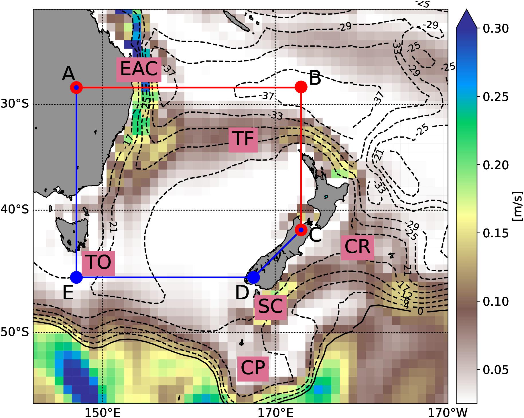
Figure 1. Modeled mean surface speed (shading) in m/s with contour lines representing the barotropic stream-function in Sv. The area enclosed by the polygon ABCDEA is the area of interest for this study, thereafter the Tasman Box. The horizontal boundaries are split into a Tasman North (red lines and dots, section ABC) and Tasman South section (blue lines and dots, section CDEA). See Table 1 for coordinates. Labels EAC, TO, TF, SC, CP and CR mark the East Australian Current, Tasman Outflow, Tasman Front, Southland Current, Campbell Plateau and Chatham Rise, respectively. The Cook Strait is the passage between New Zealand’s North and South Island near corner point C.

Marine heatwaves are characterized by prolonged periods of SST exceeding the 90th percentile of a historical baseline period (Hobday et al., 2016). MHWs in the western Tasman Sea region have been correlated with the variability of the EAC and its extension (Oliver et al., 2017, 2018a), identifying the EAC as the predominant driver of MHWs in the region. This link encourages the exploitation of ocean models to predict heatwaves based on oceanic states, such as heat content and currents. The predictive skill of ocean heat content and currents is higher than that of atmospheric variability, such as blocking high-pressure systems (which contribute to MHWs and caused the recent summer 2017/18 MHW (Salinger et al., 2019)). This is because ocean heat content variability is more persistent in time than weather patterns. Modulations in currents and heat transport due to a changing climate will impact on the heat content and thus the occurrence of MHWs in this region. Progress has been made in predicting SSTs on seasonal timescales, for winter and spring with lead times of up to 3 months (de Burgh-Day et al., 2018), but further work is required to understand precisely how the occurrence of MHWs will be affected by global warming progressing.

In this paper we investigate the connections between MHWs and meridional oceanic heat transport and content in the Tasman Sea on interannual to decadal timescales, using data from a forced ocean model and hydrographic measurements. The paper is structured as follows: section 3 describes the model, the simulation and the methodology used to compute heat content, heat transports and MHWs and provides a model evaluation.

Model, Methods, and Model Evaluation

Model Description

We use a global sea-ice coupled model to simulate the oceanic fields and investigate the links between oceanic heat content and MHWs in the Tasman Sea. The model output is based on a global forced ocean sea-ice configuration using NEMO (Madec, 2008) and CICE (Hunke and Lipscomb, 2010) as part of UKESM/NZESM (Williams et al., 2016). The global domain is defined by a coarse (nominal 1° × 1° at the equator) tripolar model grid known as eORCA1. Grid sizes in the Tasman Sea, our target region, are around 80 km. Since the model does not resolve oceanic mesoscale eddies, an eddy parameterization has been used following Gent and McWilliams (1990), with an eddy diffusivity coefficient of 2000m²/s. This configuration uses 75 vertical z-levels, with layer thickness varying between 1 m at the surface and 200 m, and with a maximum depth of 6200 m. Most (55) of the vertical layers are in the upper 2000 m. In addition, a partial cell approach has been used to improve near-bottom flows (Barnier et al., 2006). More specific model details and description of model performance of this configuration can be found in Storkey et al. (2018); Kuhlbrodt et al. (2018), and Salinger et al. (2019).

The model simulation has been started from rest, with climatological temperature and salinity values from EN4 (Good et al., 2013). Atmospheric forcing fields from JRA-55-DO version 1.3 (Tsujino et al., 2018) have been used to complete a 60-year model hindcast from 1958 to 2018. This hindcast has already been used to characterize the summer 2017/18 MHW in the Tasman Sea (Salinger et al., 2019). The modeled SSTs have been saved as daily averages, while all other oceanic fields are available as monthly means. Since the model has been started from a state of rest and with climatological values for temperature and salinity, the first 12 years of the simulation have been discarded to avoid possible spin-up effects. Therefore, time series and time averages in the manuscript are presented from 1970 onward. Coastal runoff has been prescribed with climatological values (Dai and Trenberth, 2002).

Diagnostics

Marine heatwave diagnostics (i.e., MHW area and MHW intensity) have been calculated from modeled daily SST following Hobday et al. (2016). Model data have been extracted along the four boundaries (sides) of the Tasman Sea (Figure 1) to characterize the inflows and outflows. The enclosed box, thereafter Tasman Box, covers 147° to 173°E and 46° to 28°S (Table 1), chosen to include the TF but to exclude most of the Antarctic Circumpolar Current (ACC) and the Southland Current (to avoid large variability in the south). We further split the domain into a northern boundary section (Figure 1, A-B-C), thereafter Tasman North (TN), and a southern boundary section (Figure 1, C-D-E-A), thereafter Tasman South (TS). Changes in the TN can be attributed to changes in subtropical water masses, while for TS they reflect a mixture of subtropical and subantarctic water masses (Oliver and Holbrook, 2014). Heat content and volume/heat transports have been computed from monthly mean model data. For heat transports and content, 0°C has been selected as reference temperature, and a specific heat capacity of 4000 J/kg/°K has been used. Potential density for the heat content calculation is based on modeled temperature and salinity fields. Time series have been filtered using a 23-month Hanning filter, unless otherwise stated, to eliminate the seasonal cycle. All correlation coefficients presented in this manuscript are significant at a 95% confidence interval (student t-test) and have been computed with zero time lag.

TABLE 1

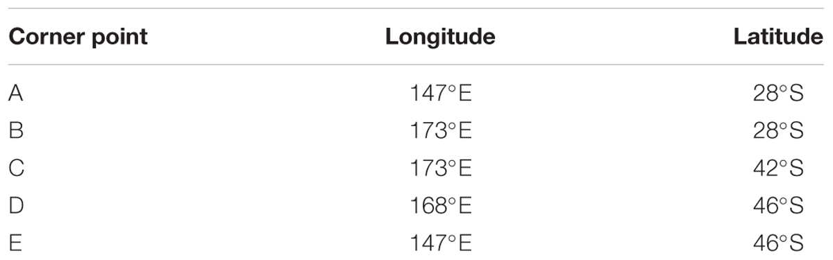
Table 1. Coordinates for corner points enclosing the Tasman Box (Figure 1).

Volume and heat transports of the EAC, TF and TO have been defined as extrema of the horizontal cumulated transports of the upper 2500 m (2000 m for TF and 3000 m for TO) over the regions, shown by cyan boxes in Figure 4. The integration starts from the coast or corner point. The TF transport is the zonal transport between corner point B and the North Cape of New Zealand and excludes transports through Cook Strait (∼0.9 Sv). The Cook Strait is the passage between New Zealand’s North and South Islands, near corner point C in Figure 1.

The modeled ocean heat content has been compared with results from the shorter time series (2004–2018) Roemmich–Gilson Argo climatology (Roemmich and Gilson, 2009). The Roemmich–Gilson product consists of optimally interpolated Argo profiles on a 1° × 1° grid of longitude and latitude and can be downloaded from http://sio-argo.ucsd.edu/RG_Climatology.html. The monthly Argo-derived temperature values extend over 58 pressure levels from the surface to 2000 m depth. In this paper, the Argo heat content is depth-integrated from 2000 m to the surface over the same region as the model results. Remotely sensed absolute dynamic topography (ADT), a multi-mission altimeter product (Ssalto/Duacs) from Archiving, Validation and Interpretation of Satellite Oceanographic data (AVISO) has been compared to modeled sea surface height (SSH) to evaluate the model and to assess the skill of remote measurements to infer heat content changes in the Tasman Sea. The Ssalto/Duacs altimeter products were produced and distributed by the Copernicus Marine and Environment Monitoring Service (CMEMS)¹. Temperature data from harmonically analyzed high-resolution expendable bathythermograph data (HRXBT) along a shipping line between Sydney and Wellington (PX34) have also been used to evaluate model data (Sutton et al., 2005). We also used large scale climate indices, the Southern Oscillation Index (SOI) and Pacific Decadal Oscillation (PDO) to investigate the influence of the principal modes of climate variability of the Pacific Ocean on MHWs in the Tasman Sea. The SOI is derived from the sea-level pressure difference between Tahiti and Darwin. The PDO is defined as the leading principal component of North Pacific monthly SST variability (poleward of 20°N for the 1900-93 period) and data have been downloaded from http://research.jisao.washington.edu/pdo/.

Model Evaluation

The mean barotropic streamfunction and surface speed shown in Figure 1 provides an impression of the large-scale ocean circulation in this model hindcast. The EAC flows southward along the east coast of Australia. South of 30°S, the EAC bifurcates into the EAC Extension, which continues south, and the TF, which flows eastward toward New Zealand. As the EAC Extension moves southward it transforms into the TO. The largest part of this outflow forms the Tasman Leakage (Ridgway and Dunn, 2007), which leaves the Tasman Sea (see corner point E in Figure 1) toward the Indian Ocean, while a second portion recirculates back into the Tasman Sea to the east.

The time mean ADT and the modeled SSH is presented in Figures 2a,b respectively. A meridional gradient is present in both datasets, elevated in the subtropics and lower in the subantarctic region. The large decrease, which is associated with the EAC Extension and TF in the northern Tasman Sea, is well represented (0.7 m contour line) in the hindcast. The central Tasman Sea shows very little change in sea surface height until near 50°S, both in the observations and simulations. Southeast of New Zealand, the Campbell Plateau shows clearly with slightly positive ADT. Flows of the Subantarctic Front along the eastern flank of the plateau are characterized by negative ADT. All these features are well represented in the modeled SSH, despite its coarse resolution. We infer from this good agreement that the near-surface ocean circulation is well captured by the model. We calculate a mean EAC volume transport of 23.3 ± 4 Sv, which is quantitatively consistent with previous reported values (Oliver and Holbrook, 2014; Sloyan and O’Kane, 2015; Ypma et al., 2016).

FIGURE 2

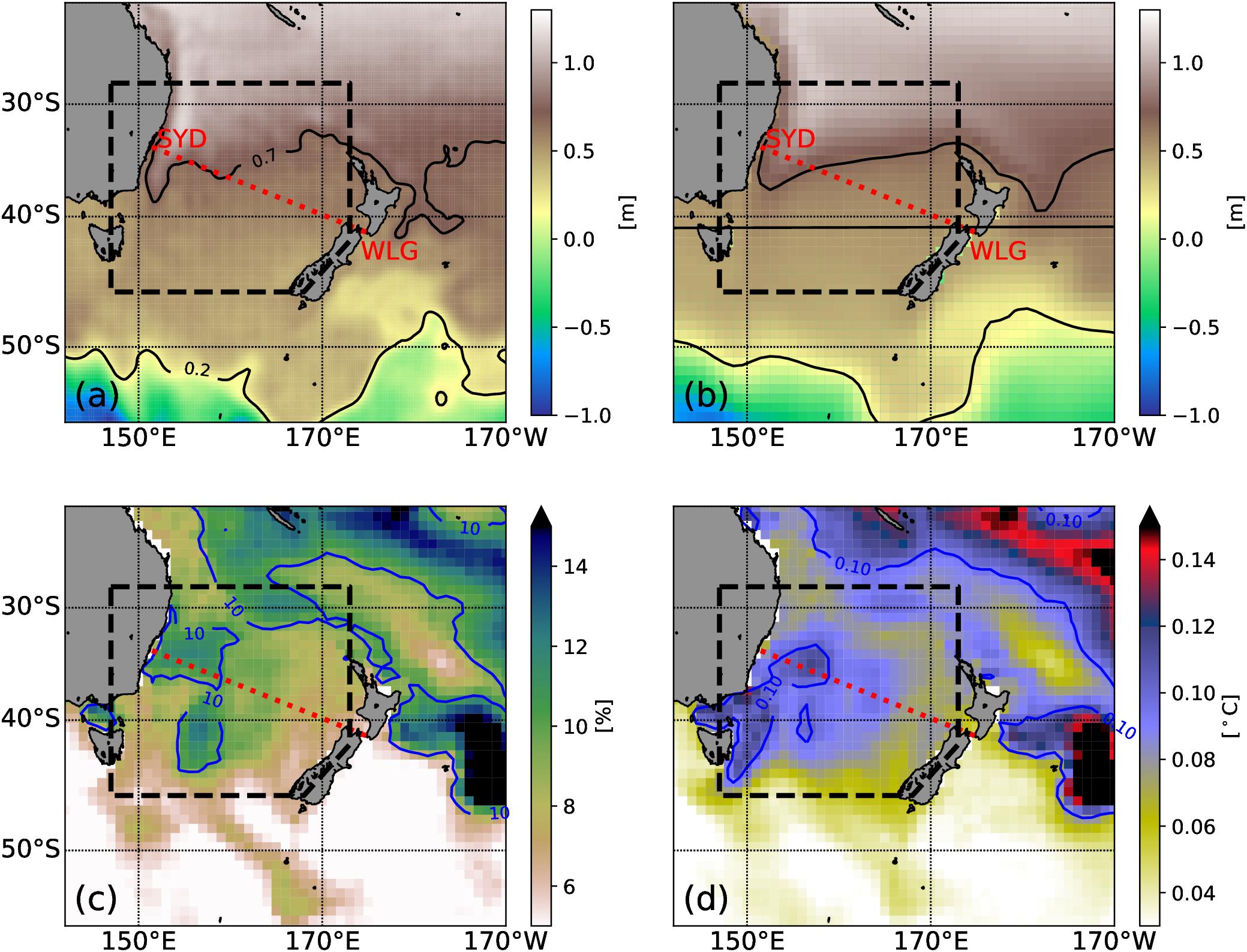
Figure 2. Mean fields (1993–2017) for (a) ADT from a multi-mission altimeter product and (b) SSH from the model hindcast. Mean probability (c) of MHW and its intensity (d) for the period 1970 to 2017. The black box illustrates the Tasman Box and the dashed red line the HRXBT transect between Wellington and Sydney (PX34). The black contour lines in (a,b) represent 0.2 and 0.7 m contour lines to aid the comparison. The blue contour lines in (c,d) represent 10% and 0.1°C contours lines.

The mean modeled MHW probability and intensity are shown in Figures 2c,d. Both diagnostics highlight that MHWs are predominantly confined to the central Tasman Sea and subtropical waters. The region south of the Tasman Sea is predominantly affected by the energetic ACC, which has a wider spectrum in the temperature climatology, therefore reducing the likelihood of MHW criteria being met. The likelihood of a MHW (Figure 2c) varies between 5 and 12% over the Tasman Sea, with hotspots in the EAC Extension, the central Tasman Sea and the eastern TF. Since defining MHWs as ocean temperatures exceeding a 90th percentile above a daily climatology, 10% would reflect the expected likelihood, without considering these conditions to last for at least 5 consecutive days. The mean MHW intensity varies between 0.05 and 0.12°C over the Tasman Sea. The regions that experience more intense MHWs are the EAC Extension, the central Tasman Sea, the northern side of the TF and the ocean south east of Tasmania. These patterns are consistent with results of previous studies (Oliver et al., 2015, 2018a,b). The HRXBT section between Wellington and Sydney (PX34) runs through the Tasman Sea (Figure 2) measuring the 0–850 m temperature approximately 4 times a year and can be used to validate the modeled mean structure and temporal variability. The mean temperature structure (for the 1991–2018 period) from the observations and the simulations is shown in Figures 3a,b respectively. In the western side of the section, the EAC, which carries warm water into the Tasman Sea, is represented by the down-sloping isotherms (Figure 3a). The modeled temperatures (Figure 3b), show similar characteristics, although the core of the EAC is not as warm as the observations suggest. This could be due to the coarse horizontal resolution of the model or due to the irregular HRXBT sampling frequency. Despite these differences, the model captures the mean temperature well, which is further demonstrated in the top 850m temperature anomaly over the section (Figure 3c). Both upper ocean heat anomalies show similar long-term variations, with the 1990s being cold and the 2000s being warmer. Both time series suggest an ongoing warming of the Tasman Sea since 2010, more evident in the observations. The larger temporal variability in the observations compared to the model can be to some extent explained by the sampling frequency of this HRXBT line.

FIGURE 3

Figure 3. Mean temperature (1991–2018) for the PX34 HRXBT transect (a) between Wellington and Sydney (see Figure 2) and (b) model hindcast. (c) top 850 m temperature anomaly over the PX34 HRXBT line from observations (blue) and model (orange). The seasonal cycle has been removed.

Overall, the model shows a good degree of consistency with observed key diagnostics in our target region, considering its coarse spatial resolution. For more regional studies, models with higher spatial resolution, which resolve mesoscale eddies, should be considered.

Results

Time Mean Properties Along the Tasman North and Tasman South Sections

In this section we assess the mean state along the northern and southern sections (TN, TS) that confine the Tasman Box. The EAC and TF dominate the TN section (Figure 1). The EAC transports warm, salty, subtropical water into the Tasman Sea and causes a zonal temperature gradient along the TN section, with the maximum temperature found near the Australian Shelf (Figure 4a). The modeled EAC occupies roughly the upper 2500m (cyan box labeled EAC). A northward recirculation to the east is part of the EAC boundary current system (Figure 4b). East of the EAC recirculation, between 1500 and 2750 km along the TN section, the upper 200m are characterized by a weak northward flow, with velocities around 1–2 cm/s. Flows associated with the TF exit the Tasman Box between corner point B and North Cape (Figure 1), represented by positive velocities (eastward flow) in the upper 2000m (cyan box labeled TF) (Figure 4b). The TF is surface-intensified and the mean modeled velocity exceeds 0.2 m/s. The heat transport of the TN section (Figure 4c) is dominated by the volume transport and consequently shows the same pattern. The EAC is the largest source of heat advection into the Tasman Sea along the TN section, while the remaining currents, in particular the TF, remove heat from the Tasman Sea. Time averaged volume (and heat transports) for the EAC of -23.3 ± 4 Sv (-1273 ± 232 PW) are in the range of results provided in earlier studies (Oliver and Holbrook, 2014; Sloyan and O’Kane, 2015; Ypma et al., 2016; Bull et al., 2017). Mean transports for the TF of 19.8 ± 3.6 Sv (888 ± 134 PW) are about twice as large. However, the net outflow from the Tasman Sea across the TN is comparable with earlier studies. Those studies suggest a different split for the volume transports, between TF and northward transport across AB than this model hindcast. Their AB outflow is larger, ranges between 8 and 18 Sv, and results to a smaller TF transport.

FIGURE 4

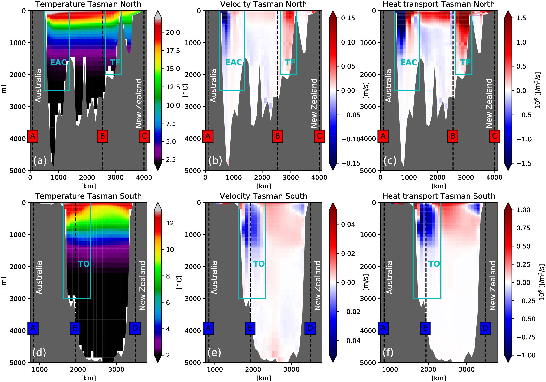
Figure 4. Time averaged (1970–2017) quantities along Tasman North (ABC) and Tasman South section (CDEA). (a,d) Temperature in °C, (b,e) cross section velocity in m/s and (c,f) heat transport in 10⁶ J/m²/s. Specific currents have been labeled, with TF (Tasman Front), EAC (East Australian Current) and TO (Tasman Outflow). In addition the boundary points of the Tasman box have been labeled with (A)-(E). Gray shaded area is the model bathymetry. Transports follow the common sign convention where positive transports show northward or eastward transports. Segments A-B and D-E show meridional transports, while B-C and E toward Australia are zonal transports.

The TS section is dominated by the TO (Ridgway and Godfrey, 1994), which feeds the Tasman Leakage (Ridgway and Dunn, 2007), and a flow which recirculates back into the Tasman Sea south of Tasmania. This bifurcation was seen in the barotropic streamfunction contour lines in Figure 1. The outflow originates from the EAC and is the reason for the warm temperatures close to Tasmania (Figure 4d). The modelled TO extend down to about 3000 m and is sub-surface intensified, with its maximum around 800–1000 m (Figure 4e). The subsurface intensification was also found in earlier studies (Ridgway and Dunn, 2007; van Sebille et al., 2012). Model current speeds of roughly 3–4 cm/s and the total transport of 9.9 ± 4.6 Sv are consistent with other studies (Ridgway, 2007; Hill et al., 2011). At the surface near the New Zealand West Coast, a weak flow associated with the STF is directed southward and then skirts southern New Zealand as a precursor to the Southland Current (Chiswell et al., 2015). Heat transport follows the volume transport (Figure 4f) and identifies the TO as the southern export pathway of heat for the Tasman Sea. While some of this heat recirculates back into the Tasman Sea, a substantial portion is carried into the Indian Ocean.

The vertical profiles of mean horizontal transports for the sections are shown in Figure 5a. While the net volume transport across both sections totals to a mean southward flow of roughly -3.3 Sv, approximately the upper 150m of both sections show a northward-directed flow. That is due to the fact that the modeled TF and Cook Strait transport overcompensates the southward transport of the EAC in the near-surface layer (dashed line). Below this transition depth, the net transport is southward throughout the rest of the water column, with a distinct extremum in the TS section at around 850m, representing the TO (Ridgway and Dunn, 2007). The net southward transport of about -3.3 Sv through the Tasman Sea is on the lower end of the range suggested by other studies for the TO (usually around 6–7 Sv, Oliver and Holbrook, 2014; Ypma et al., 2016).

FIGURE 5

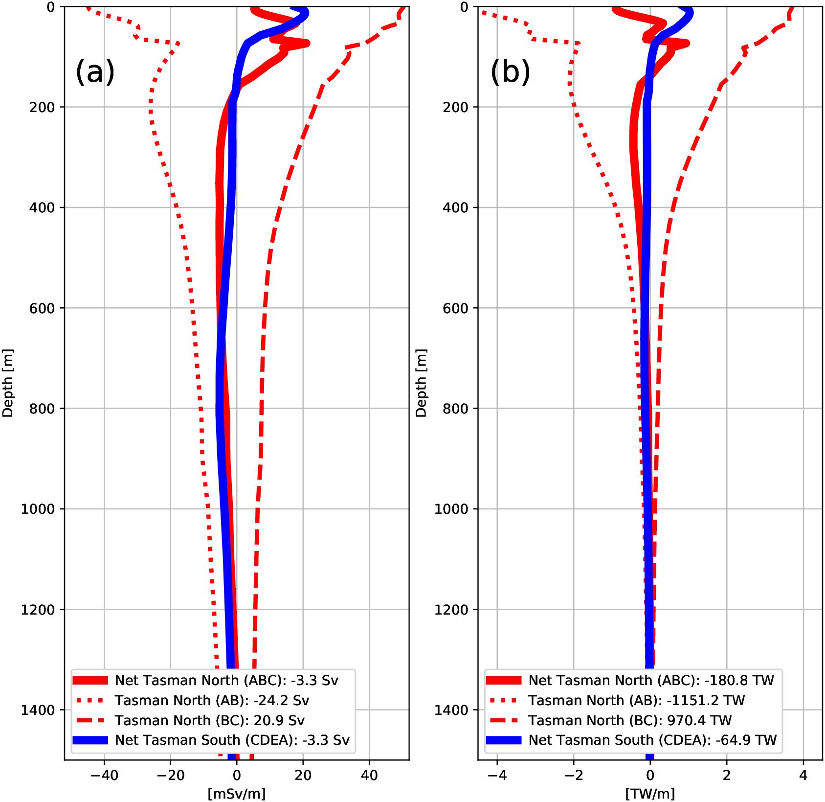
Figure 5. Vertical profiles for time mean (1970–2018) (a) volume and (b) heat transport for sections TN and TS. Red (blue) curves show cross section transports for the Tasman North (South) section. Net transports are shown as solid thick lines. Positive (negative) values for Tasman North (South) reflect transports leaving the Tasman Sea across this boundary. Mean values are provided in the legend.

With knowledge of the volume transports, the modeled heat transport profile is easier to understand (Figure 5b). Due to the large heat transport of the TF (dashed line), the net heat transport of the TN section is not entirely southward as could be expected. Between 30 and 150 m the TF and Cook Strait extract heat from the Tasman Sea, while heat is carried into the Tasman Sea both shallower and deeper. The reversal in heat transport, from northward to southward, is located in the TS section at approximately 150 m. The difference between 180.8 TW along TN and 64.9 TW along TS (Figure 5b) reflects a large atmospheric heat flux of approximately 115 TW over the Tasman Box to balance the heat transport convergence. Considering the area of the Tasman Box, this is equivalent to a mean net heat flux of around 22 W/m² to the atmosphere, which is in agreement with values from heat flux reanalysis (not shown).

Variability of Volume and Heat Transport and Its Impact on Heat Content

Earlier studies found a relationship between volume transports of EAC, TF and TO/EAC-Extension (Hill et al., 2011; Sloyan and O’Kane, 2015), with increased EAC transports corresponding to increased TF and lower EAC-Extension transports. Here, EAC and TF transports on interannual time scales are correlated at r = 0.6. For TO/EAC-Extension and TF transports, the anti-correlation varied from r = -0.6 to r = -0.8 for different data products on decadal time scales. Our modeled transports (Figure 6) also show an anti-correlation between TF and TO using annual means, with slightly a lower correlation coefficient (r = -0.48).

FIGURE 6

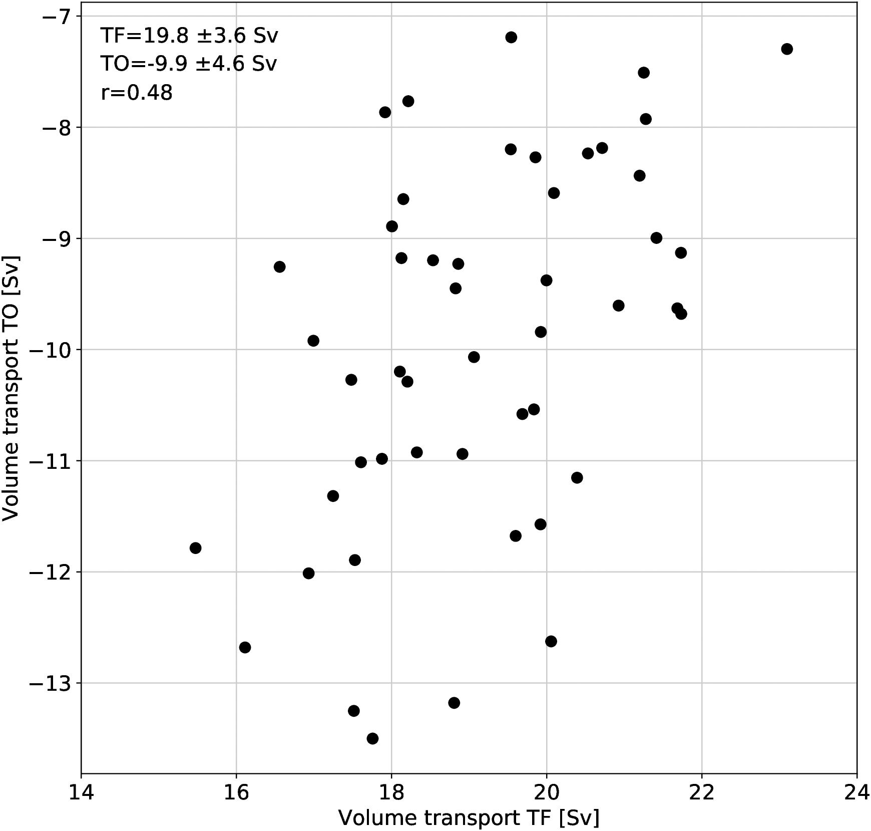
Figure 6. Annual mean modeled volume transports for TF and TO, showing the gating between both transport pathways supplied by the EAC.

We now investigate the interannual variability of transports across TN and TS and compare the transports to heat content changes in the Tasman Box. Transports of TN and TS reflect transports across the entire section. For transports of EAC and TF the cyan boxes in Figure 4 have been used as regional limits. The time average over the period from 1970 to 2017 has been used as a reference to derive anomalies, except for the ADT and Argo anomalies, where 1993 to 2017 and 2004 to 2017 have been used, respectively. The volume transport anomalies of TN and TS (Figure 7a) present significant interannual to decadal variability. The period from 2003 to 2013 is characterized with an ongoing decline in transport and relatively little interannual variability in both sections. Sloyan and O’Kane (2015) also described lower EAC transports from 2000 to 2004 and lower TF transports from 2000 to the end of their record (2008). Most of the volume transport variability of TN and TS results from the complex interplay between the EAC and TF transports (EAC-TF, black curve). This is reflected in the good alignment between variability across both sections and the difference between the EAC and TF (thick black line) with a correlation of r = 0.88. Note this difference is obtained by subtracting the individual time averages of EAC and TF from 1970 to 2017 prior to the subtraction. The EAC and TF transports show general co-variability, in agreement with previous studies (Sloyan and O’Kane, 2015), but the TF exhibits larger interannual variability than the EAC (standard deviation of 2.4 Sv versus 1.6 Sv). Here the very large modeled transport of TF is potentially contributing to this large variability. This co-variability (r = -0.42) only emerges when the time series are interannually filtered and is not present in the annual averages.

FIGURE 7

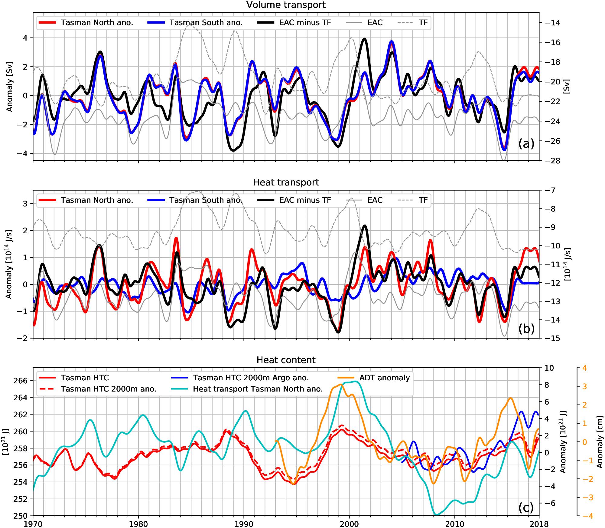
Figure 7. Interannual filtered time series: (a) volume transport, (b) heat transport and (c) heat content (HTC). (a) Volume transport anomaly for the Tasman North (red) and Tasman South (blue) section and difference between EAC and Tasman Front (black). Transports of Tasman North and South reflect transports across the entire section. For transports of EAC and TF the cyan boxes in Figure 4 have been used as regional limits. For anomalies the time mean values from 1970 to 2017 have been used as reference. Net transports for EAC and TF are represented in thin gray lines and use the right hand y-scale. Note that, the sign for TF transport in (a,b) has been inverted. (b) Heat transport anomalies and net heat transports, as in (a). (c) Tasman Sea heat content: full-depth (solid red line, left hand y-scale) and upper 2000 m anomalies (red dashed line, inner right hand y-scale). Heat content anomaly derived from the integrated Northern Tasman section heat transport (light blue line, linear de-trended, inner right hand y-scale). Argo-derived heat content anomaly (dark blue line, inner right hand y-scale) and absolute dynamic topography (ADT, orange line, linear de-trended, in cm and outer right hand y-scale).

For the heat transport across TN and TS (Figure 7b), the characteristics are similar to the volume transport, with the order of 90% of the interannual variability of the TN section (red) being attributed to the heat transport differences between the EAC and TF (black). The period from 2003 to approximately 2013 again stands out, with relatively low interannual variability compared with earlier periods. The heat transport variations across the TS section are smaller compared to TN (standard deviation of 0.7 10¹⁴ J/s vs. 0.9 10¹⁴ J/s), as a result of the colder sub-antarctic water masses being advected, while volume transport variations are the same. The heat transports of the EAC and TF show the same co-variability (r = -0.6) as the volume transports. Quantitatively, the EAC imports more heat into the Tasman Sea than is exported by the TF and other outflows along TN, with the imbalance being compensated by atmospheric fluxes, heat content changes and heat transport across TS.

As shown above, the heat transport across the TN section is dominating the heat transport into the Tasman Sea and thus the heat content and its variability (Figure 7c). The heat transport across TS only accounts for around 30% of that across TN. Full depth and upper 2000m heat content are linked and show similar variability to the heat content changes, because of the heat transport across the TN section (light blue line in Figure 7c). The heat content drop in the early 1990s stands out from the time series in terms of intensity and persistence. This drop is present in the TN transports, as is the rebound in the late 1990s and is consistent with temperature observations along PX34 (Sutton et al., 2005 and Figure 3c). The modeled upper 2000m heat content is correlated to the Argo-derived heat content (r = 0.7) in the Tasman Sea (blue line) and shows a positive trend since early 2010, which is within the range of natural variability. From 2015 onward, the modeled heat content is consistently lower than the Argo-derived heat content, while both timeseries share similar variability. Reasons for this mismatch remain unknown, but suggest that the model underestimates the heat extremes during this period. The ADT anomaly (shown by the orange curve) correlates (r = 0.7) with heat content, since heat content changes affects the steric component, suggesting that heat content changes can be inferred from remotely sensed observations on interannual to decadal time scales. This provides an opportunity to establish a near real-time measure for inferring heat content trends in the Tasman Sea and therefore a measure for the likelihood of MHWs.

To explain the origin of the variability of the TN heat transport, we computed the correlation of the TN heat transport with the wind stress curl from JRA-55-DO (Figure 8). The correlation coefficient shows a zonal band of positive correlations north of the TN boundary and negative correlations south of it. The coefficients are in the order of r = ± 0.25 over most of the region. In this regard, the positive heat transport anomalies coinciding with positive wind stress curl anomalies between 30°S and 20°S suggest an acceleration of the western boundary current (i.e., the EAC), according to the Sverdrup balance (Sverdrup, 1947), the Island Rule (Godfrey, 1989) and recent studies built on them (Cai, 2006; Hill et al., 2008; Bull et al., 2017, 2018). Without additional wind stress curl changes over the Tasman Sea, both the TF and EAC-Extension heat and volume transports will increase to balance the EAC. In a steady state, the heat content over the Tasman Sea would remain unchanged. However, the negative correlation over most of the Tasman Sea (Figure 8) reflects a decrease in wind stress curl and a weaker transport of the EAC-Extension and TO. In this case the TF partially compensates the transport anomaly of the EAC-Extension, but the imbalance may explain the Tasman heat content rise which is in line with previous studies focusing on wind-driven changes on the EAC, EAC Extension and TF (Hill et al., 2010; Oliver and Holbrook, 2014; Sloyan and O’Kane, 2015; Bull et al., 2017). We note that this response is only caused by non-uniform wind stress curl anomalies between 20°S and 30°S and over the Tasman Sea, in particular the negative anomalies over the Tasman Sea. Recent studies show a positive wind stress curl trend over the entire region, due to intensified westerlies, which leads to an enhanced EAC-Extension transport (Matear et al., 2013; Oliver and Holbrook, 2014; Qu et al., 2018). The drivers for TF variability or outflow across TN and how it balances the heat transport of the EAC, are less well established, with more detailed work required to investigate this sensitive and important balance.

FIGURE 8

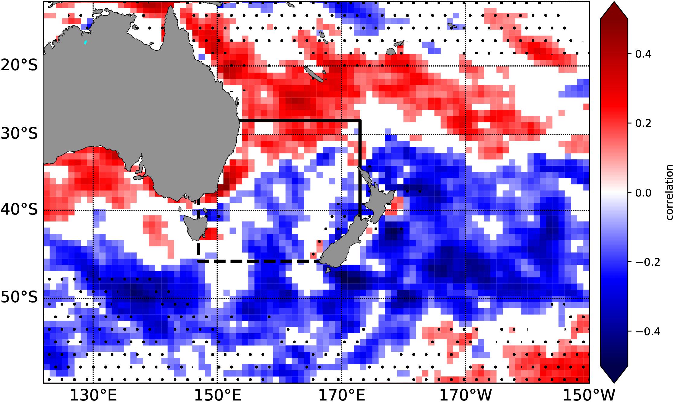
Figure 8. Correlation between Tasman North heat transport and wind stress curl over the period 1970 to 2017 (interannually filtered). Only significant correlations above the 95% confidence level are shown. The dots indicate regions with a negative mean wind stress curl. The Tasman Box is shown by the black lines. The Tasman North section is marked by the solid black line and Tasman South by the dashed black line.

Furthermore, we investigate the vertical coherence of the heat content anomaly, its temporal change and heat transport anomaly across the TN section (Figure 9). A time-averaged profile from 1970 to 2017 has been used to compute the anomalies. The temporal evolution of the depth-dependent heat content suggests a separation into three layers: above 250m, between 250 and 750 m and below 750 m. The top 250 m shows a positive–negative alternating signal with downward propagating anomalies through this depth range. In this layer, the 1990s are characterized by a distinct cool phase, followed by a warm phase between 1997 and 2002 and from 2012 until present. The depth of 250 m roughly corresponds to the depth where the net heat transport of TN is southward in the mean vertical profile (see Figure 5b). The layer between 250 and 750 m is characterized by warming until 2000 which then leveled off. The layer below 750m shows the opposite behavior, with a warm phase until 1990, cooling until 2010 and little change afterward.

FIGURE 9

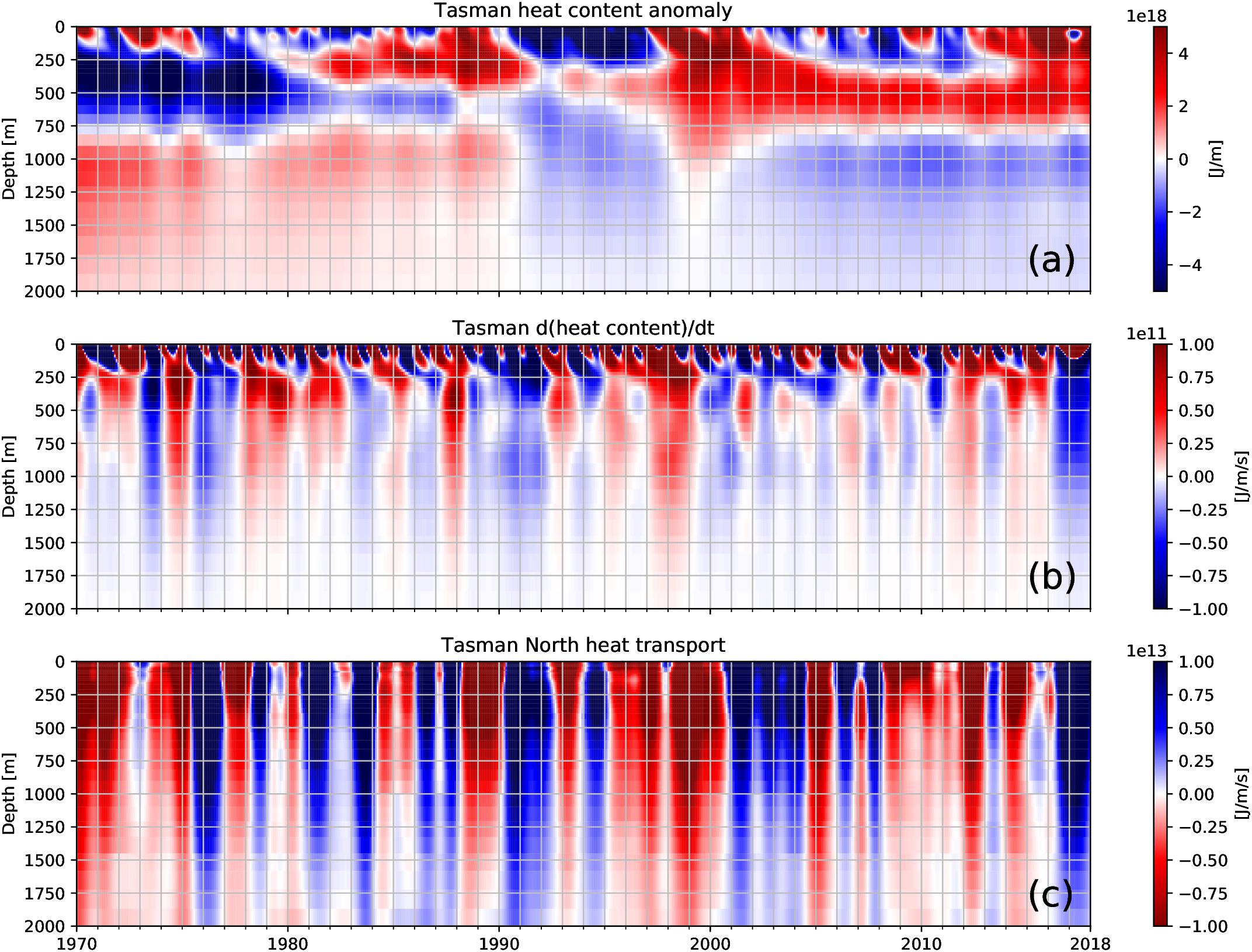
Figure 9. Vertical profiles of (a) Tasman Box heat content anomaly, (b) Tasman Box heat content change and (c) TN heat transport anomalies, interannually filtered. The time averaged profile from 1970 to 2017 has been used as the reference for computing anomalies. Please note the inverted color scale in (c). All anomalies have been normalized using the vertical model layer thickness.

Computing the temporal change of the heat content anomaly, we obtain strongly barotropic anomalies below 200m, despite the three layers (Figure 9b). Most of these anomalies can be connected to heat transport anomalies along TN (Figure 9c). Note that the colorscale in Figure 9c has been inverted, therefore positive anomalies (blue) indicate that heat is transported out of the Tasman Box across the TN section. The consequence is that the heat content change in Figure 9b is negative (blue) and vice versa for negative anomalies. This underpins again the dominant role of the heat transport across TN in the Tasman heat content variability.

Heat Content and MHW

In this section we investigate the relationships between the Tasman Box heat content and MHWs. There is a direct connection via SSTs, since SSTs are used to characterize MHWs and are also typically correlated with upper ocean heat content. However, predicting SSTs and thus MHWs months ahead is challenging due to large atmospheric variability resulting in low predictive skill (Palmer and Anderson, 1994; Doblas-Reyes et al., 2013; de Burgh-Day et al., 2018). Integrated quantities such as heat content show lower variability and an enhanced predictive skill. This is demonstrated in the close agreement between Tasman Sea heat content and the area identified as MHW (Figure 10a). Periods with either a positive heat content anomaly or a sudden increase in heat content correspond with periods where larger parts of the Tasman Sea are under MHW conditions.

FIGURE 10

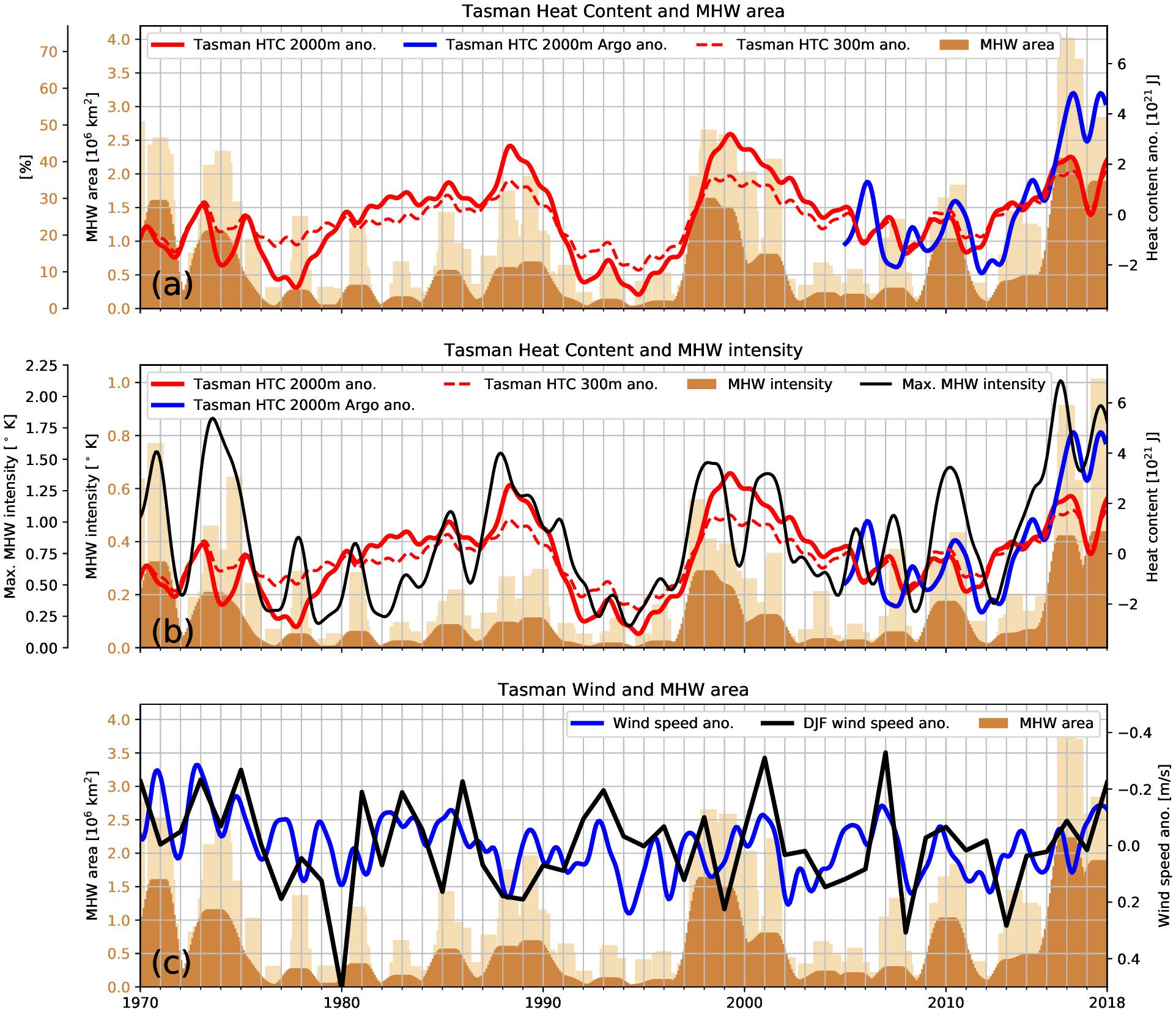
Figure 10. Link between depth-integrated Tasman Box heat content and occurrence of MHWs in the Tasman Sea. (a) Upper 2000 m (300 m) heat content in red (red dashed) and area (in 10⁶ km²) identified as marine heatwave as light brown bars (monthly means) and fraction (%) of the Tasman Box (inner and outer left hand y scales). Dark brown area is MHW area interannually filtered. The Argo-derived heat content anomaly is shown in dark blue. (b) As for (a), but area-averaged MHW intensity represented by light brown bars (monthly means) and interannually filtered dark brown. Black line shows the maximum MHW intensity over the Tasman Box. (c) Area averaged wind speed and December-January-February (DJF) mean anomalies (in blue and black, respectively) and total area identified as in marine heatwave conditions in (light) brown as in (a). All time series have been interannually filtered, except the light brown monthly MHW data and DJF wind anomaly in (c).

The period between 1970 and 1974 shows two sudden increases in heat content, with an increased MHW area during that period, with a short drop around 1972. From 1975 to 1989 the ocean heat content keeps slowly increasing. Despite the steady increase of the heat content, with values exceeding the early 1970s, the MHW area is smaller. However, periods where the ocean heat content increases more strongly than the long-term trend (i.e., 1981, 1985, 1988–1989) have associated MHW activity. From 1989, the heat content decreases rapidly until 1995, with very few signs of MHWs seen during that period. After 1995, the heat content increases sharply, reaching a maximum around the year 1999, with correspondingly larger areas under MHW conditions. The heat content decreases afterward until 2009 and the Tasman Sea experiences less MHW activity, except for 2010 when the heat content increases rapidly. The upward trend of the heat content since 2011 is then reflected in large parts of the Tasman Sea being under MHW conditions. Although the ocean heat content increase after 2015 has leveled off, the MHW activity is still high. The correlation between modeled 2000m depth-integrated heat content and MHW area reaches r = 0.35, when the heat content is leading by 4 months. For the top 300m modeled heat content and MHWs, the correlation increases as expected to r = 0.46 (ocean heat content leading by 4 months) since the SST contribution becomes more important for a shallower (300m) heat content. The correlation for the Argo-derived heat content and the occurrence of MHWs is r = 0.43 with heat content leading by 5 months. The difference in correlation coefficient of model and Argo-derived heat content with MHWs is influenced by the different record length. Although heat content alone does not explain every individual marine heatwave event (e.g., the MHW of the Summer 2017/18 appears (Salinger et al., 2019) to have different characteristics compared to the previous one in 2015/2016), these results suggest that heat content has predictive skill down to even annual timescales, and certainly captures long-term (multi-year) modulations.

Not only can the area of MHWs be inferred from heat content, but also the MHW intensity, as shown in Figure 10b. The link with area-averaged intensity appears to be stronger than that with the MHW area, and periods of larger heat content (e.g., early 2000, 2008–2012, and since 2014) can be connected to MHW intensity. The maximum of the MHW intensity over the Tasman Sea correlates with the oceanic heat content (r = 0.7) and for Argo-derived heat content over the top 2000m (r = 0.66). Using area-averaged wind speeds or austral summer anomalies (DJF) over the Tasman Sea (Figure 10c) to infer the vertical mixing or surface heating, which has been found to drive some MHWs (e.g., Summer 2017/18, Salinger et al., 2019), does not provide a robust measure to infer MHWs. No significant relationship has been found between wind speeds and MHWs on longer time scales. Surface winds contribute to the development of MHWs directly, since they affect air–sea fluxes and vertical mixing. Only a few MHW events (i.e., 2001, 2007 and 2018) appear to be dominated by low winds.

The coupling between ocean heat content and MHW area becomes more apparent when just considering annual maximum values for the Tasman Sea (Figure 11). Note that annual values refer to the period from June through May, to center diagnostics on the Southern Hemisphere summer, i.e., 2000 refers to the period from June 1999 to May 2000). The correlation coefficient between the annual maximum value for heat content and MHW area is r = 0.43 (Figure 11a). According to this diagnostic, the 2015/16 MHW (labeled 2016) covered the largest area and was the most intense MHW, while the 2017/18 (labeled 2018) was less intense. There was also a period between June 2016 and May 2017 (labeled 2017) where large parts of the Tasman Sea were under MHW condition but with lower intensity and impact.

FIGURE 11

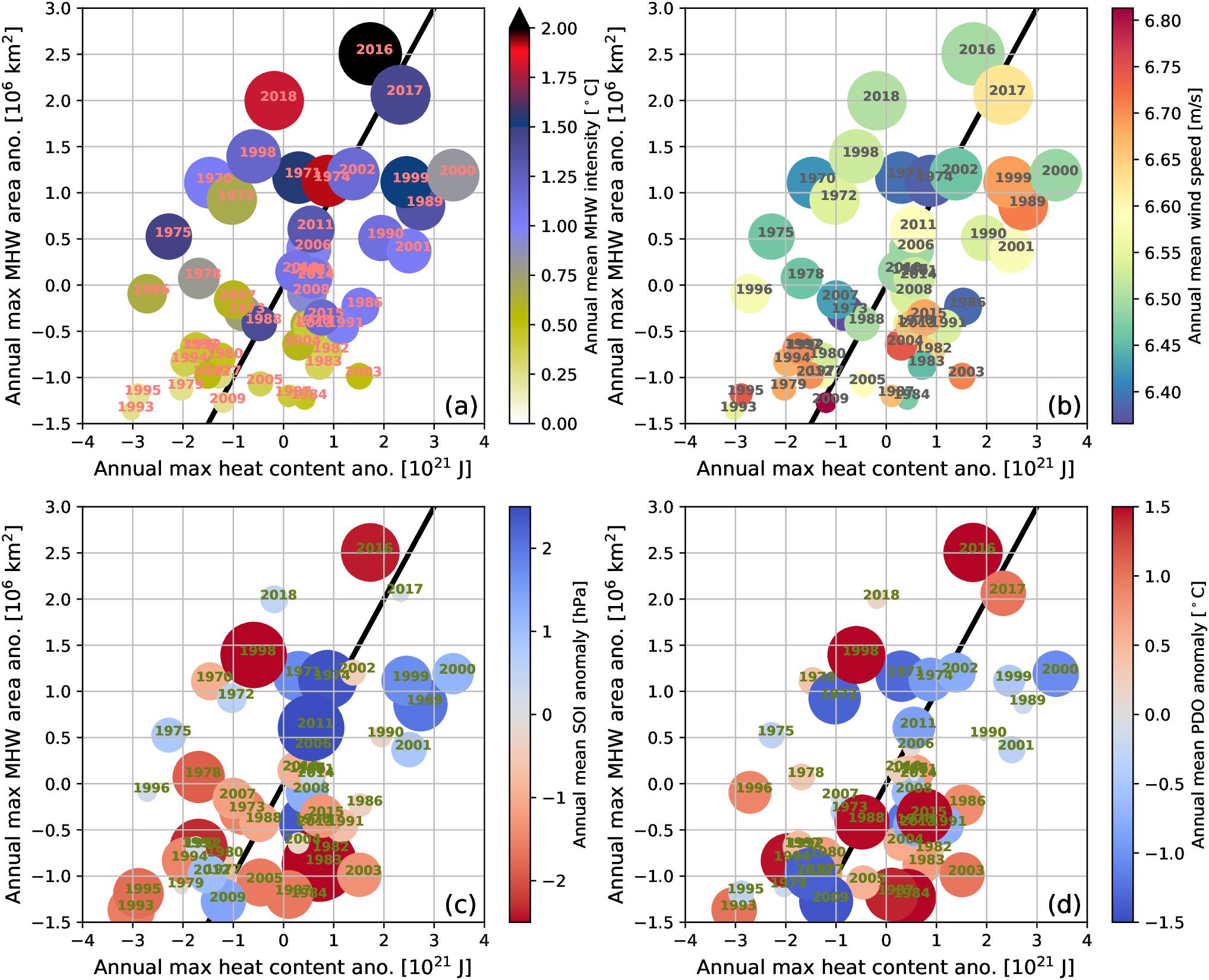
Figure 11. Link between upper ocean heat content and area of MHWs on annual basis. Scatter plot shows annual maximum of heat content (x-axis) and annual maximum MHW area (y-axis), over the Tasman Box (a–d). Annual averages are centered on Southern Hemisphere summers, for example maximum/mean values for 2000 cover the period from June 1999 through to May 2000. (a,b) size of the circles is proportional to the annual maximum MHW area (y-axis), while color indicates (a) annual mean MHW intensity and (b) annual mean wind speed. (c,d) as for (a,b) but size and color of circles show annual mean SOI anomaly (c) and PDO anomaly (d).

A possible explanation for why this 2017 MHW was not as severe is indicated by the wind diagnostics, which show that 2017 had stronger winds than 2016 and 2018 (Figure 11b). Strong winds would have caused more vertical mixing of heat into the water column. Comparing Figures 11a,b shows the complexity of individual drivers for MHWs. Many years with negative ocean heat content anomaly can still show intense and large MHWs (e.g., 1975, 1998, 2018), which can be attributed to lower winds and reduced vertical mixing of heat into the water column. In these cases, the surface ocean heats up more than usual and the background state, i.e., ocean heat content, is less important for the development of MHW conditions. Conversely, in years with positive heat content anomalies, the background state becomes more important. There are a few exceptions from this generalization on both sides of the regression line (e.g., 2000), highlighting that more factors also need to be taken into account (e.g., cloudiness). According to the described mechanism, the year 2000 should also have been a MHW year, due to low winds and large positive heat content anomaly. Here, it is likely the timing of these maxima also needs to be taken into account, adding another layer of complexity. MHWs occur all year round, but surface heating, which is essential for the development of MHWs, is only strong during austral spring and summer months. If favorable conditions occur during other periods of the year, the weaker surface heating will result in milder MHW conditions compared to what would have occurred during austral spring and summer.

It is worth noting that modeled ocean heat content over the last few years is lower than it has been in the past (i.e., 1989, 1999–2001), which would imply that MHWs have not been as intense as they could have been. However, with SSTs and heat content showing an upward trend over the last decades in the Tasman Sea (Roemmich et al., 2015; Sutton and Bowen, 2019), we could soon reach those higher heat content values again, resulting in more intense MHWs.

Time series presented in Figures 7, 10 show large interannual to decadal variability. It is therefore tempting to try to link them with large-scale weather patterns such as El Niño Southern Oscillation (ENSO) and PDO (Pacific Decadal Oscillation), as done in Figures 11c,d. Previous studies suggested only a very weak ENSO signal is present in the EAC volume transport (Ridgway, 2007) and consequently in the heat transport. Note that we use the SOI as a measure for the ENSO state. A positive SOI index reflects a larger pressure difference between Tahiti and Darwin; stronger trade winds; and La Niña like conditions, where positive SSTs anomalies are located in the west Pacific. A negative SOI describes El Niño conditions, lower trade winds, and positive SSTs anomalies in the east Pacific. Results for the heat content and MHW in combination with ENSO do not show a conclusive pattern (Figure 11c). If the positive SST anomalies during La Niña conditions reached into the Tasman Sea or caused an enhanced heat transport of the EAC, the heat content should be elevated, and the converse would be seen for El Niño conditions (Figure 11c). The years 1989 and 1999–2001 are years with strong La Niña conditions, positive ocean heat content anomalies and MHWs. However, there are several years which show positive heat content anomalies and El Niño conditions (e.g., 1982, 1988). Likewise, little consistency can be seen for negative heat content anomalies, which could occur during El Niño conditions. Therefore, links between ENSO, Tasman Sea heat content and MHWs are not conclusive. The same applies if we perform the same diagnostic for the PDO, another leading index describing long-term variability in the Pacific (Figure 11d). The PDO SST pattern and impact are ENSO-like but on longer time scales. Positive PDOs describe El Niño-like and negative La Niña-like conditions. Similarly to the SOI results, little consistency can be found between the PDO state and MHWs and no preferred heat content state can be identified for either positive or negative PDOs.

Discussion and Conclusion

In this manuscript we investigated the connection between ocean heat content, heat transport and the area and intensity of MHWs in the Tasman Sea, on interannual to decadal timescales, by using a coarse-resolution forced ocean hindcast corroborated by optimally interpolated data from Argo, satellite measurements and in situ HRXBT temperature observations. The model results show that meridional heat transports from the subtropics dominate heat content fluctuations in the Tasman Sea. The Tasman Sea is a region of oceanic heat convergence, meaning that average surface heat fluxes are directed toward the atmosphere to balance the oceanic heat convergence. On average around 67% of the ocean heat transported from the subtropics into the Tasman Sea fuels surface heat fluxes.

The heat transport variability from the subtropics is impacted by regional wind stress curl anomalies in this area, which influence the volume and thus the heat transport of the EAC, following Sverdrups’ and Godfrey’s Island Rule theories. We show that heat transport of TF needs to be considered for the heat content budget of the Tasman Sea. The TF’s contribution to balance the heat transport of the EAC, which is in the order of 85%, is overestimated in our model, due to the overly strong mean volume transport of the TF. Nevertheless, even with half of its modeled contribution it provides a significant portion to the heat budget across TN. A smaller portion does not necessarily affect its temporal variability and interplay with EAC heat transport anomalies, which has been found to control the heat content changes in the Tasman Sea. Volume and heat transport of the TF are usually in phase with the EAC on interannual time scales, in agreement with observations (Hill et al., 2008; Sloyan and O’Kane, 2015). Despite the coarse horizontal resolution of the model, which is not eddy-resolving, volume and heat transports for EAC and TO are within the range of previous studies. We do note that our modeled TF transport is about twice that of previous studies (e.g., Oliver and Holbrook (2014)), while the overall transport which leaves the Tasman Box across the TN sections is in agreement. That reflects that our model shows a different split between TF transports and transports east of the EAC along the AB section of TN. Here the choice of the location of corner point B could play a role. Our choice was motivated by the modeled barotropic streamfunction (Figure 1), which suggested little flow around corner point B. While the position is in broad agreement with the other studies, a southward shift of corner point B would have resulted in a transport shift from TF toward the transports east of the EAC. Despite the discrepancy in the mean transports of TF, the long-term variability is in agreement (i.e., co-variability between EAC and TO). Furthermore, the model is able to robustly simulate observed variability in the Tasman Sea compared to HRXBT and satellite altimetry observations. For more detailed studies and finer regional focus, models which are capable of resolving mesoscales should be considered, but this is beyond the scope of this study.

We could not find a robust link between Tasman Sea heat content variability and the large-scale climate patterns of ENSO and the PDO on interannual to decadal time scales. Potentially their influence is not instantaneous through direct local wind changes but affects the heat content through Rossby and Kelvin wave propagation (Bowen et al., 2017). More detailed work is required here.

Our model results and data from Argo show a robust link between Tasman Sea heat content (upper 2000 m) and MHWs, in terms of the area under MHW conditions and MHW intensities on interannual to decadal time scales. The heat content acts as a preconditioner for the development of MHWs. Periods with enhanced heat content or when ocean heat content increases rapidly increase the likelihood of MHWs developing. Periods where the heat content anomalies are negative show less MHW activity. Ocean heat content alone cannot explain every MHW in the Tasman Sea, since strong surface heating can also trigger MHWs, as seen in the MHW in Austral Summer 2017/18. Here, exceptionally low winds over the Tasman Sea led to a reduction in vertical mixing and caused the SSTs to exceed MHW thresholds, while the heat content was almost unchanged relative to previous years (Salinger et al., 2019). Nevertheless, ocean heat content is a measure for the background state of the ocean and if the ocean is already warm then less surface heating is required to develop MHW conditions.

This demonstrates that there are at least two different mechanisms affecting the occurrence of MHWs in the Tasman Sea: the oceanic background state (e.g., heat content), which is persistent and enables better predictability, and the atmospheric forcing (e.g., winds, surface heating), which usually acts on shorter timescales and is thus harder to predict. In the former case, the predictability of heat content changes is further enhanced since the driving mechanisms of EAC dynamics are well understood. Predictability could be further enhanced if a robust understanding of the TF dynamics/outflow from the Tasman Box across TN and its variability were developed. This would reduce the uncertainties in the EAC–TF heat transport difference, or in other words the net heat transport across TN, which sets the heat content of the Tasman Sea in our model.

Author Contributions

EB performed this study. DF and PS helped with the interpretation of the results, supported the writing process, and delivered time series for this study.

Funding

This study obtained funding from Deep South National Science Challenge (Oceans Projects), Marsden Funds (17-NIW-005) and NIWA (CAOC1805).

Conflict of Interest Statement

The authors declare that the research was conducted in the absence of any commercial or financial relationships that could be construed as a potential conflict of interest.

Acknowledgments

HRXBT data were made available by the Scripps High Resolution XBT program http://www-hrx.ucsd.edu. The Argo data were collected and made freely available by the International Argo Program and the national programs that contribute to it (http://www.argo.ucsd.edu, http://argo.jcommops.org). The Argo Program is part of the Global Ocean Observing System. The Roemmich and Gilson Argo climatology was accessed from http://sio-argo.ucsd.edu/RG_Climatology.html. ADT data has been provided through https://cds.climate.copernicus.eu/cdsapp#!/dataset/satellite-sea-level-global?tab=overview, generated using Copernicus Atmosphere Monitoring Service Information 2018. The data for the SOI index originates from Trenberth, Kevin & National Center for Atmospheric Research Staff (Eds). Last modified 11 Jan 2019. “The Climate Data Guide: Southern Oscillation Indices: Signal, Noise and Tahiti/Darwin SLP (SOI).” Retrieved from https://climatedataguide.ucar.edu/climate-data/southern-oscillation-indices-signal-noise-and-tahitidarwin-slp-soi. We acknowledge Pat Hyder’s (MetOffice) and Adam Blaker’s (NOC) contributions to this study. In addition we thank Frances Boyson for the proofreading and constructive comments.

Footnotes

1. ^http://marine.copernicus.eu/

References

Barnier, B., Gurvan, M., Thierry, P., Jean-Marc, M., Anne-Marie, T., Julien, L. E. S., et al. (2006). Impact of partial steps and momentum advection schemes in a global ocean circulation model at eddy-permitting resolution. Ocean Dyn. 56, 543–567. doi: 10.1007/s10236-006-0082-1

CrossRef Full Text | Google Scholar

Bowen, M., and Markham, J. (2017). Interannual variability of sea surface temperature in the Southwest Pacific and the role of ocean dynamics. J. Clim. 30, 7481–7492. doi: 10.1175/JCLI-D-16-0852.1

CrossRef Full Text | Google Scholar

Bowen, M., Markham, J., Sutton, P., Zhang, X., Wu, Q., Shears, N., et al. (2017). Interannual variability of sea surface temperature in the southwest pacific and the role of ocean dynamics. J. Clim. 30, 7481–7492. doi: 10.1175/JCLI-D-16-0852.1

CrossRef Full Text | Google Scholar

Bull, C. Y. S., Kiss, A. E., Jourdain, N. C., England, M. H., and van Sebille, E. (2017). Wind forced variability in eddy formation, eddy shedding, and the separation of the east australian current. J. Geophys. Res. Ocean 122, 9980–9998. doi: 10.1002/2017JC013311

CrossRef Full Text | Google Scholar

Bull, C. Y. S., Kiss, A. E., van Sebille, E., Jourdain, N. C., and England, M. H. (2018). The role of the new zealand plateau in the tasman sea circulation and separation of the east australian current. J. Geophys. Res. Ocean 123, 1457–1470. doi: 10.1002/2017JC013412

CrossRef Full Text | Google Scholar

Cai, W. (2006). Antarctic ozone depletion causes an intensification of the Southern Ocean super-gyre circulation. Geophys. Res. Lett. 33:L03712. doi: 10.1029/2005GL024911

CrossRef Full Text | Google Scholar

Cetina-Heredia, P., Roughan, M., Van Sebille, E., and Coleman, M. A. (2014). Long-term trends in the East Australian Current separation latitude and eddy driven transport. J. Geophys. Res. Ocean 119, 4351–4366. doi: 10.1002/2014JC010071

CrossRef Full Text | Google Scholar

Chiswell, S. M., Bostock, H. C., Sutton, P. J., and Williams, M. J. (2015). Physical oceanography of the deep seas around New Zealand: a review. New Zeal. J. Mar. Freshw. Res. 49, 1–32. doi: 10.1080/00288330.2014.992918

CrossRef Full Text | Google Scholar

Church, J. A., and White, N. J. (2006). A 20th century acceleration in global sea-level rise. Geophys. Res. Lett. 33:L01602. doi: 10.1029/2005GL024826

CrossRef Full Text | Google Scholar

Dai, A., and Trenberth, K. E. (2002). Estimates of freshwater discharge from continents: latitudinal and seasonal variations. J. Hydrometeorol. 3, 660–687. doi: 10.1175/1525-7541(2002)003<0660:eofdfc>2.0.co;2

CrossRef Full Text

de Burgh-Day, C. O., Spillman, C. M., Stevens, C., Alves, O., and Rickard, G. (2018). Predicting seasonal ocean variability around New Zealand using a coupled ocean-atmosphere model. New Zeal. J. Mar. Freshw. Res. 53, 201–221. doi: 10.1080/00288330.2018.1538052

CrossRef Full Text | Google Scholar

Demaria, M., Kaplan, J., Demaria, M., and Kaplan, J. (1994). Sea surface temperature and the maximum intensity of Atlantic tropical cyclones. J. Clim. 7, 1324–1334. doi: 10.1175/1520-04421994007<1324:SSTATM<2.0.CO;2

CrossRef Full Text | Google Scholar

Doblas-Reyes, F. J., García-Serrano, J., Lienert, F., Biescas, A. P., and Rodrigues, L. R. L. (2013). Seasonal climate predictability and forecasting: status and prospects. Wiley Interdiscip. Rev. Clim. Chang. 4, 245–268. doi: 10.1002/wcc.217

CrossRef Full Text | Google Scholar

Fang, M., and Zhang, J. (2015). Basin-scale features of global sea level trends revealed by altimeter data from 1993 to 2013. J. Oceanogr. 71, 297–310. doi: 10.1007/s10872-015-0289-1

CrossRef Full Text | Google Scholar

Feng, M., Zhang, X., Oke, P., Monselesan, D., Chamberlain, M., Matear, R., et al. (2016). Invigorating ocean boundary current systems around Australia during 1979–2014: as simulated in a near-global eddy-resolving ocean model. J. Geophys. Res. Ocean 121, 3395–3408. doi: 10.1002/2016JC011842

CrossRef Full Text | Google Scholar

Gent, P. R., and McWilliams, J. C. (1990). Isopycnal mixing in ocean circulation models. J. Phys. Oceanogr. 20, 150–155. doi: 10.1175/1520-04851990020<0150:IMIOCM<2.0.CO;2

PubMed Abstract | CrossRef Full Text | Google Scholar

Godfrey, J. S. (1989). A sverdrup model of the depth-integrated flow for the world ocean allowing for island circulations. Geophys. Astrophys. Fluid Dyn. 45, 89–112. doi: 10.1080/03091928908208894

CrossRef Full Text | Google Scholar

Godfrey, J. S., Cresswell, G. R., Golding, T. J., Pearce, A. F., Boyd, R., Godfrey, J. S., et al. (1980). The separation of the East Australian Current. J. Phys. Oceanogr. 10, 430–440. doi: 10.1175/1520-04851980010<0430:TSOTEA<2.0.CO;2

CrossRef Full Text | Google Scholar

Good, S. A., Martin, M. J., and Rayner, N. A. (2013). EN4: quality controlled ocean temperature and salinity profiles and monthly objective analyses with uncertainty estimates. J. Geophys. Res. Ocean 118, 6704–6716. doi: 10.1002/2013JC009067

CrossRef Full Text | Google Scholar

Hannah, J., and Bell, R. G. (2012). Regional sea level trends in New Zealand. J. Geophys. Res. Ocean 117:C01004. doi: 10.1029/2011JC007591

PubMed Abstract | CrossRef Full Text | Google Scholar

Herring, S. C., Hoerling, M. P., Kossin, J. P., Peterson, T. C., Stott, P. A., Herring, S. C., et al. (2015). Explaining extreme events of 2014 from a climate perspective. Bull. Am. Meteorol. Soc. 96, S1–S172. doi: 10.1175/BAMS-ExplainingExtremeEvents2014.1

CrossRef Full Text | Google Scholar

Hill, K. L., Rintoul, S. R., Coleman, R., and Ridgway, K. R. (2008). Wind forced low frequency variability of the East Australia Current. Geophys. Res. Lett. 35:L08602. doi: 10.1029/2007GL032912

CrossRef Full Text | Google Scholar

Hill, K. L., Rintoul, S. R., Oke, P. R., and Ridgway, K. (2010). Rapid response of the east australian current to remote wind forcing: the role of barotropic-baroclinic interactions. Mar. J. Res. 68, 413–431. doi: 10.1357/002224010794657218

CrossRef Full Text | Google Scholar

Hill, K. L., Rintoul, S. R., Ridgway, K. R., and Oke, P. R. (2011). Decadal changes in the South Pacific western boundary current system revealed in observations and ocean state estimates. J. Geophys. Res. 116:C01009. doi: 10.1029/2009JC005926

CrossRef Full Text | Google Scholar

Hobday, A. J., Alexander, L. V., Perkins, S. E., Smale, D. A., Straub, S. C., Oliver, E. C. J., et al. (2016). A hierarchical approach to defining marine heatwaves. Prog. Oceanogr. 141, 227–238. doi: 10.1016/J.POCEAN.2015.12.014

CrossRef Full Text | Google Scholar

Hu, D., Wu, L., Cai, W., Gupta, A. S., Ganachaud, A., Qiu, B., et al. (2015). Pacific western boundary currents and their roles in climate. Nature 522, 299–308. doi: 10.1038/nature14504

PubMed Abstract | CrossRef Full Text | Google Scholar

Hunke, E., and Lipscomb, W. (2010). CICE: The Los Alamos Sea Ice Model, Documentation and Software User’s Manual, Version 4.1, (LA-CC-06–012).

Google Scholar

Johnson, C. R., Banks, S. M., and Barrett, N. S. (2011). Climate change cascades: shifts in oceanography, species’ ranges and subtidal marine community dynamics in eastern Tasmania. J. Exp. Mar. Biol. Ecol. 400, 17–32. doi: 10.1016/J.JEMBE.2011.02.032

CrossRef Full Text | Google Scholar

Kuhlbrodt, T., Jones, C. G., Sellar, A., Storkey, D., Blockley, E., Stringer, M., et al. (2018). The low-resolution version of HadGEM3 GC3.1: development and evaluation for global climate. J. Adv. Model. Earth Syst. 10, 2865–2888. doi: 10.1029/2018MS001370

PubMed Abstract | CrossRef Full Text | Google Scholar

Kuleshov, Y., Qi, L., Fawcett, R., and Jones, D. (2008). On tropical cyclone activity in the southern hemisphere: trends and the ENSO connection. Geophys. Res. Lett. 35:L14S08. doi: 10.1029/2007GL032983

CrossRef Full Text | Google Scholar

Madec, G. (2008). NEMO the Ocean Engine. Note du Pole de Modélisation. France: Institut Pierre-Simon Laplace.

Matear, R. J., Chamberlain, M. A., Sun, C., and Feng, M. (2013). Climate change projection of the tasman sea from an eddy-resolving ocean model. J. Geophys. Res. Ocean 118, 2961–2976. doi: 10.1002/jgrc.20202

CrossRef Full Text | Google Scholar

Oliver, E. C. J., Benthuysen, J. A., Bindoff, N. L., Hobday, A. J., Holbrook, N. J., Mundy, C. N., et al. (2017). The unprecedented 2015/16 Tasman Sea marine heatwave. Nat. Commun. 8:16101. doi: 10.1038/ncomms16101

PubMed Abstract | CrossRef Full Text | Google Scholar

Oliver, E. C. J., Donat, M. G., Burrows, M. T., Moore, P. J., Smale, D. A., Alexander, L. V., et al. (2018a). Longer and more frequent marine heatwaves over the past century. Nat. Commun. 9:1324. doi: 10.1038/s41467-018-03732-9

PubMed Abstract | CrossRef Full Text | Google Scholar

Oliver, E. C. J., Lago, V., Hobday, A. J., Holbrook, N. J., Ling, S. D., and Mundy, C. N. (2018b). Marine heatwaves off eastern Tasmania: trends, interannual variability, and predictability. Prog. Oceanogr. 161, 116–130. doi: 10.1016/J.POCEAN.2018.02.007

CrossRef Full Text | Google Scholar

Oliver, E. C. J., and Holbrook, N. J. (2014). Extending our understanding of south pacific gyre “spin-up”: modeling the East Australian Current in a future climate. J. Geophys. Res. Ocean 119, 2788–2805. doi: 10.1002/2013JC009591

CrossRef Full Text | Google Scholar

Oliver, E. C. J., O’Kane, T. J., and Holbrook, N. J. (2015). Projected changes to Tasman Sea eddies in a future climate. J. Geophys. Res. Ocean 120, 7150–7165. doi: 10.1002/2015JC010993

CrossRef Full Text | Google Scholar

Oliver, E. C. J., Wotherspoon, S. J., Chamberlain, M. A., and Holbrook, N. J. (2014). Projected Tasman Sea extremes in sea surface temperature through the twenty-first century. J. Clim. 27, 1980–1998. doi: 10.1175/JCLI-D-13-00259.1

CrossRef Full Text | Google Scholar

Palmer, T. N., and Anderson, D. L. T. (1994). The prospects for seasonal forecasting—a review paper. Meteorol. Q. J. R. Soc. 120, 755–793. doi: 10.1002/qj.49712051802

CrossRef Full Text | Google Scholar

Purich, A., Cowan, T., Min, S. K., and Cai, W. (2013). Autumn precipitation trends over southern hemisphere midlatitudes as simulated by CMIP5 models. J. Clim. 26, 8341–8356. doi: 10.1175/JCLI-D-13-00007.1

CrossRef Full Text | Google Scholar

Qu, T., Fukumori, I., and Fine, R. A. (2018). Spin-up of the southern hemisphere super gyre. J. Geophys. Res. Ocean 124, 154–170. doi: 10.1029/2018JC014391

CrossRef Full Text | Google Scholar

Ridgway, K. R. (2007). Long-term trend and decadal variability of the southward penetration of the East Australian Current. Geophys. Res. Lett. 34:L13613. doi: 10.1029/2007GL030393

CrossRef Full Text | Google Scholar

Ridgway, K. R., and Dunn, J. R. (2007). Observational evidence for a southern hemisphere oceanic supergyre. Geophys. Res. Lett. 34:L13612. doi: 10.1029/2007GL030392

CrossRef Full Text | Google Scholar

Ridgway, K. R., and Godfrey, J. S. (1994). Mass and heat budgets in the East Australian Current: a direct approach. J. Geophys. Res. 99, 3231–3248. doi: 10.1029/93JC02255

CrossRef Full Text | Google Scholar

Roemmich, D., Church, J., Gilson, J., Monselesan, D., Sutton, P., and Wijffels, S. (2015). Unabated planetary warming and its ocean structure since 2006. Nat. Clim. Chang 5, 240–245. doi: 10.1038/nclimate2513

CrossRef Full Text | Google Scholar

Roemmich, D., and Gilson, J. (2009). The 2004–2008 mean and annual cycle of temperature, salinity, and steric height in the global ocean from the Argo Program. Prog. Oceanogr. 82, 81–100. doi: 10.1016/J.POCEAN.2009.03.004

CrossRef Full Text | Google Scholar

Salinger, J., Renwick, J., Behrens, E., Mullan, A. B., Diamond, H. J., Sirguey, P., et al. (2019). The unprecedented coupled ocean-atmosphere summer heatwave in the New Zealand region 2017/18: drivers, mechanisms and impacts. Environ. Res. Lett. 14:044023. doi: 10.1088/1748-9326/ab012a

CrossRef Full Text | Google Scholar

Shears, N. T., and Bowen, M. M. (2017). Half a century of coastal temperature records reveal complex warming trends in western boundary currents. Sci. Rep. 7:14527. doi: 10.1038/s41598-017-14944-2

PubMed Abstract | CrossRef Full Text | Google Scholar

Sloyan, B. M., and O’Kane, T. J. (2015). Drivers of decadal variability in the Tasman Sea. J. Geophys. Res. Ocean 120, 3193–3210. doi: 10.1002/2014JC010550

CrossRef Full Text | Google Scholar

Sloyan, B. M., Ridgway, K. R., Cowley, R., Sloyan, B. M., Ridgway, K. R., and Cowley, R. (2016). The East Australian Current and property transport at 27°S from 2012 to 2013. J. Phys. Oceanogr. 46, 993–1008. doi: 10.1175/JPO-D-15-0052.1

CrossRef Full Text | Google Scholar

Sokolov, S., and Rintoul, S. R. (2009). Circumpolar structure and distribution of the Antarctic Circumpolar Current fronts: 1. mean circumpolar paths. J. Geophys. Res. 114:C11018. doi: 10.1029/2008JC005108

CrossRef Full Text | Google Scholar

Speich, S., Blanke, B., de Vries, P., Drijfhout, S., Döös, K., Ganachaud, A., et al. (2002). Tasman leakage: a new route in the global ocean conveyor belt. Geophys. Res. Lett. 29, 55–51. doi: 10.1029/2001GL014586

CrossRef Full Text | Google Scholar

Stammer, D. (1997). Global characteristics of ocean variability estimated from regional TOPEX/POSEIDON altimeter measurements. J. Phys. Oceanogr. 27, 1743–1769. doi: 10.1175/1520-04851997027<1743:GCOOVE<2.0.CO;2

CrossRef Full Text | Google Scholar

Stanton, B., and Sutton, P. (2003). Velocity measurements in the East Auckland Current north-east of North Cape, New Zealand. New Zeal. J. Mar. Freshw. Res. 37, 195–204. doi: 10.1080/00288330.2003.9517157

CrossRef Full Text | Google Scholar

Stanton, B. R. (2010). An oceanographic survey of the Tasman Front. New Zeal. J. Mar. Freshw. Res. 15, 289–297. doi: 10.1080/00288330.1981.9515924

CrossRef Full Text | Google Scholar

Stanton, B. R., Sutton, P. J. H., and Chiswell, S. M. (1997). The East Auckland Current, 1994–95. New Zeal. J. Mar. Freshw. Res. 31, 537–549. doi: 10.1080/00288330.1997.9516787

CrossRef Full Text | Google Scholar

Storkey, D., Blaker, S. T., Mathiot, P., Megann, A., Aksenov, Y., Blockley, E. W., et al. (2018). UK global ocean GO6 and GO7: a traceable hierarchy of model resolutions. Geosci. Model Dev. 11, 3187–3213. doi: 10.5194/gmd-11-3187-2018

CrossRef Full Text | Google Scholar

Sutton, P. J. H., and Bowen, M. (2014). Flows in the Tasman Front south of Norfolk Island. J. Geophys. Res. Ocean 119, 3041–3053. doi: 10.1002/2013JC009543

CrossRef Full Text | Google Scholar

Sutton, P. J. H., and Bowen, M. (2019). Ocean temperature change around New Zealand over the last 36 years. New Zeal. Mar. J. Freshw. Res. 1–22. doi: 10.1080/00288330.2018.1562945

CrossRef Full Text | Google Scholar

Sutton, P. J. H., Bowen, M., and Roemmich, D. (2005). Decadal temperature changes in the Tasman Sea. New Zeal. J. Mar. Freshw. Res. 39, 1321–1329. doi: 10.1080/00288330.2005.9517396

CrossRef Full Text | Google Scholar

Sverdrup, H. U. (1947). Wind-driven currents in a baroclinic ocean; with application to the equatorial currents of the eastern Pacific. Proc. Natl. Acad. Sci. U.S.A. 33, 318–326. doi: 10.1073/pnas.33.11.318

PubMed Abstract | CrossRef Full Text | Google Scholar

Swart, N. C., and Fyfe, J. C. (2012). Observed and simulated changes in the southern hemisphere surface westerly wind-stress. Geophys. Res. Lett. 39:L16711. doi: 10.1029/2012GL052810

CrossRef Full Text | Google Scholar

Tsujino, H., Urakawa, S., Nakano, H., Small, J., Kim, W. M., Yeager, S. G., et al. (2018). JRA-55 based surface dataset for driving ocean–sea-ice models (JRA55-do). Ocean Model. 130, 79–139. doi: 10.1016/J.OCEMOD.2018.07.002

CrossRef Full Text | Google Scholar

van Sebille, E., England, M. H., Zika, J. D., and Sloyan, B. M. (2012). Tasman leakage in a fine-resolution ocean model. Geophys. Res. Lett. 39:L06601. doi: 10.1029/2012GL051004

CrossRef Full Text | Google Scholar

Williams, J., Morgenstern, O., Varma, V., Behrens, E., Hayek, W., Oliver, H., et al. (2016). Development of the New Zealand Earth System Model: NZESM. Weather Clim. 36, 25–44.

Google Scholar

Ypma, S. L., van Sebille, E., Kiss, A. E., and Spence, P. (2016). The separation of the East Australian Current: a lagrangian approach to potential vorticity and upstream control. J. Geophys. Res. Ocean 121, 758–774. doi: 10.1002/2015JC011133

CrossRef Full Text | Google Scholar