Going Beyond Standard Ocean Color Observations: Lidar and Polarimetry

Introduction

Since the inception of ocean color satellite observation systems, remote sensing has been based on measurements of the radiance emerging at the top of the Ocean color remote sensing utilizes the intensity and spectral variation of visible light scattered upward from beneath the ocean surface to derive concentrations of biogeochemical constituents and inherent optical properties within the ocean surface layer. Passive ocean color space-borne observations began in the late 1970s with the launch of the CZCS space mission. An uninterrupted record of global ocean color data has been sustained since 1997 (thanks to SeaWiFS, MODIS-AQUA, MERIS, VIIRS and OLCI sensors) and will continue at least until 2035 with the NASA/PACE and ESA/Sentinel-3 space missions. These passive observations have enabled a global view of the distribution of marine particles [phytoplankton, total suspended matter (TSM) and colored dissolved organic matter (CDOM), McClain (2009)]. However, these measurements are limited to clear sky, day-light, high Sun elevation angles, and are exponentially weighted toward the ocean surface. Moreover, the processing of the ocean color images requires the knowledge of the atmospheric components (gases, air molecules and aerosols). This step can induce errors (IOCCG, 2010; Jamet et al., 2011; Goyens et al., 2013 among others). Only non- or weakly-absorbing aerosols are accounted for, preventing monitoring some areas over long periods (dust over West coasts of Africa and Arabian Sea; pollution over East coasts of US and coasts of China).

Observations of aerosols use different passive and active remote sensing techniques that could be applied to the ocean for better characterizing the hydrosols and also to improve the atmospheric correction processing. Among those techniques, two are very promising: polarimetry and lidar (Neukermans et al., 2018).

While the spectral radiance is sensitive to absorption and scattering properties of the constituents within the water column, polarized light emerging from the Earth system carries a plethora of information about the atmosphere, ocean, and its surface that is currently underutilized in ocean color remote sensing. Polarized light originating from below the ocean surface contains microphysical information about hydrosols such as their shape, composition, and attenuation, which is difficult if not impossible to retrieve from traditional scalar remote sensing alone. Additionally, polarimetric measurements can be utilized to improve the characterization and removal of atmosphere and surface reflectance that confounds the ocean color measurement. Optical polarimetric remote sensing methods have been extensively used to study the full characteristics of the microphysical properties of suspended particles in the atmosphere, namely aerosols and cloud droplets. The development of sensors capable of measuring and quantifying the polarization characteristics of light scattered by the atmosphere-ocean (AO) system is becoming increasingly important and is opening a new frontier for understanding climate variables. Several space agencies worldwide, including the National Aeronautics and Space Administration (NASA), Centre National d'Etudes Spatiales (CNES), European Space Agency (ESA), and Japanese Aerospace Exploration Agency (JAXA), have launched space observing polarimetric instruments to study aerosols and clouds. These efforts include NASA APS instrument oboard the Glory mission (Mishchenko et al., 2007), the CNES POLDER/PARASOL satellite instruments (Fougnie et al., 2007), and JAXA's SGLI on board GCOM-C (Honda et al., 2006). The aerosol and cloud science communities make increasing use of polarimetric remote sensing to constrain atmospheric particle properties of importance to climate and radiative forcing (Riedi et al., 2010; Dubovik et al., 2011; Hasekamp et al., 2011; Lacagnina et al., 2015; Marbach et al., 2015; Wu et al., 2016; Xu et al., 2016, 2017), but application to ocean color science has been limited, despite a long history of sporadic research in this area. Waterman (1954) was the first to study the underwater polarization as a function of illumination and viewing geometry, while Ivanoff et al. (1961) showed a high degree of polarization in clear ocean waters. It was decade later that Timofeyeva (1970) first demonstrated a decreased degree of polarization in more turbid waters, based on laboratory measurements. Kattawar et al. (1973) pioneered the vector radiative transfer simulations of a coupled atmosphere-ocean system, and 30 years passed before Chowdhary et al. (2006) first modeled the polarized ocean contribution specifically for photopolarimetric remote sensing observations of aerosols above the ocean (Chowdhary et al., 2012), after which interest in ocean applications intensified. Chami (2007) has shown the potential advantage of utilizing polarimetry in understanding the optical and microphysical properties of suspended oceanic particles (hydrosols), based on Radiative Transfer (RT) simulations. Tonizzo et al. (2009) developed a hyperspectral, multiangular polarimeter to measure the polarized light field in the ocean accompanied by an RT closure analysis validating the theoretical analysis. Voss and Souaidia (2010) were able to measure the upwelling hemispheric polarized radiance at several visible wavelengths showing the geometrical dependence of polarized light. Adams et al. (2002) did a closure study in which they matched the measured polarized radiance in clear Mediterranean waters with Monte Carlo RT simulations employing a simple ocean-atmosphere optical model. Although practical utilization and field measurements of the ocean polarized light to retrieve ocean inherent optical properties (IOPs) have been limited, a plethora of theoretical RT models have been developed and utilized for research. Several fully coupled vector radiative transfer (VRT) models that can simulate photopolarimetric radiative transfer through the atmosphere and ocean and across the interface have been constructed and are in current use. These VRT models use various schemes such as Monte Carlo (Kattawar et al., 1973; Cohen et al., 2013), Adding-Doubling (Hansen and Travis, 1974; Takashima and Masuda, 1985; Chowdhary et al., 2006), Discrete Ordinate method (Stamnes et al., 1988; Schulz et al., 1999), Successive Order of Scattering (SOS) (Ahmad and Fraser, 1982; Lenoble et al., 2007; Zhai et al., 2009), Markov chain (Xu et al., 2011) and Multi-Component Approximation (Zege et al., 1993). The 3 × 3 approximation in VRT can be used to accurately simulate the reflected and transmitted total radiance, I, and the polarized radiances Q and U in the atmosphere-ocean system for an unpolarized source such as the Sun (Hansen, 1971; Stamnes et al., 2017). More details are provided in section Polarimetry Technique.

Lidar is the acronym of Light Detection and Ranging. Lidar is a “laser radar” technique that has been used for a wide range of atmospheric applications (Measures, 1984; Weitkamp, 2006) including measurements of aerosols, clouds, atmospheric trace gases and surface elevation. For ocean applications, lidar has been mainly employed from aircraft (Churnside, 2014 and references within). Lidar allows the estimation of the shallow water depth along coastal waters with a high accuracy and high spatial density features (Guenther et al., 2000; Hiddale and Raff, 2007; Bailly et al., 2010). Lidar also has a better penetration into the seawater, up to three times that of passive sensors (Peeri et al., 2011). Abdallah et al. (2013) studied two scenarios for spaceborne bathymetric lidar: an ultra-violet (UV) lidar and a green lidar. Their waveform simulations showed that the bathymetry detection rate at a 1 m depth varied between 19 and 54% for the UV lidar and between 0 and 22% for the green lidar depending of the type of waters. They also showed that the lidar accuracy, when the depth is detected, was around 2.8 cm. Lidar has been widely used for fisheries. The first detection of fish schools was shown by Murphree et al. (1974), followed by several additional studies (e.g., Squire and Krumboltz, 1981). Airborne (Vasilkov et al., 2001) or ship-borne lidar (Bukin et al., 2001) have been also used to detect scattering layers over the depth. It is also a very promising technique for the estimation of the sea temperature profiles using either the Raman or the Brillouin scattering (Leonard et al., 1979; Rudolf and Walther, 2014 and references within) but these studies were either theoretical development or laboratory tests. As the lidar equation (section Basics of Lidar) is a function of the scattering and absorption coefficients of the marine particles, it is therefore possible to detect the optical properties of the seawater (Churnside et al., 1998; Montes et al., 2011). More detailed examples of the use of airborne lidar in oceanic applications is shown in section Polarization Lidar.

Despite the oceanic applications of lidar (as shown previously and more in details in section Lidar technique), this active remote sensing technique has not received significant attention from the ocean color remote sensing community. Several reasons can explain this: cost and size of the instrument, lack of sampling swath, few wavelengths, etc. However, this technique has regained interest from the ocean community in the past years. New studies used the lidar signal from the space-borne CALIOP instrument on-board CALIPSO to estimate particulate backscatter (Behrenfeld et al., 2013, 2017; Churnside et al., 2013; Lu et al., 2014) and show that the lidar signal from CALIOP provides accurate estimates of this parameter over the globe. However, the CALIOP instrument was not designed for ocean applications and its coarse vertical resolution makes the retrieval of vertically-resolved ocean properties challenging. In addition, the standard backscatter technique employed in CALIOP does not enable the separation of vertical variation in absorption and from that of scattering. New technologies such as the High-Spectral Resolution Lidar (HSRL; Hair et al., 2008, 2016; Hostetler et al., 2018) can help to overcome this issue [section High-Spectral-Resolution Lidar (HSRL)].

Presently, there is a major need to develop a lidar and polarimetry ocean community with access to ship and/or aircraft in-situ instruments. There is also a major need to develop outreach and education programs (e.g., through summer schools and curriculum) to develop a new generation of remote sensing scientists and engineers trained in lidar and polarimetry techniques (section Outreach and Education). Two main summer schools are organized for Msc/PhD students and early career scientists working on ocean color (University of Maine and IOCCG, respectively). However, no specific or polarimetry courses are included in their curriculum. This is mainly due to lack of available instruments and scientists being able to teach oceanic lidar.

In this review, polarimetry and lidar are presented for applications in ocean into two separate sections, with their theoretical description followed by examples of results. A third section shortly presents the need in term of education and outreach.

Lidar Technique

Basics of Lidar

Oceanographic lidars can be configured to implement several different measurement techniques (described below) but all rely on the same basic principle of operation (see, for instance, Hoge, 2003, 2005; Churnside, 2014; Hostetler et al., 2018). A laser transmitter emits a short (e.g., 10 ns) pulse of light into the water. This light pulse interacts with the marine particles (water molecules, phytoplankton, suspended particulate matter) in ways that either scatter the transmitted photons or generate photons at different wavelengths through absorption and re-emission. A small portion of these photons travel backward toward the lidar where they are collected by an optical telescope. Optical components downstream of the telescope collimate the received light and optically separate it into various optical channels as dictated by the particle technique being implemented. Optical detectors and signal processing electronics respond to the received optical power and convert it to a digital signal, which is recorded as a function of time from the initiation of the laser pulse. The time-of-flight ranging technique is used to convert this time-profile into a profile as a function of range or depth: i.e., the “clock” starts at the initiation of the laser pulse, and the distance that photons have traveled is determined by the speed of light; photons arriving later come from greater distances than photons arriving earlier. The range resolution of a lidar profile is determined by the rate of sampling by its detection electronics: the higher the rate, the higher the range resolution. Oceanographic lidars are typically operated in a nadir or near-nadir pointing geometry such that they provide depth-resolved profile information.

The most common laser source is the Q-switched, frequency-doubled Nd:YAG laser, operating at 532 nm. This wavelength is chosen due to the robustness of available lasers, not as the optimum wavelength for ocean remote sensing. Gray et al. (2015) characterized the benefits to use a multi-wavelength lidar (470/490 nm and ~570 nm) for improving depth penetration with wavelengths.

In-situ Lidar

By “in-situ” marine lidars, we refer to lidars that are operated below the sea surface (in-water) or just above (above-water) it from ships or other marine vehicles. Advances in lidar technology, making it more and more rugged, compact, energy efficient, and inexpensive, have increased the use of in-situ lidar in marine studies. Regular deployment of these systems on a variety of platforms becomes increasingly practical, allowing for continuous remote sensing of the vertical and horizontal distribution of particles in the ocean. Some basic requirements of in-situ marine lidars include the following.

1. A watertight, compact, modular and mechanically robust enclosure system to protect optical and electronic components from water and sea salt.

2. A rugged, vibration-insensitive laser transmitter that can operate under the required environmental conditions (e.g., variation in temperature) and a structure that can insure maintenance of transmitter-to-receiver alignment.

3. A receiver with optical filtering bandwidth and stability required and to spectrally select the return signals of interest (this can be done through interference filters as well as spectrometers or interferometers, depending on the required spectral resolution). For ocean lidar applications, a large detection dynamic range is required (for fluorescence applications (described below) this is not as critical). Finally, a high signal sampling rate is required when small/vertical-scale structures are to be investigated.

Depending on the objectives of the particular application, the in-situ lidar systems constructed and deployed can satisfy the aforementioned requirements to a different extent. Typically, the in-situ lidar configurations can be identified on the basis of the interaction between radiation and matter used by the lidar systems. The mostly common configurations are: (1) Elastic backscatter lidar and (2) Light Induced Fluorescence lidar. We also present some results from newer multi-spectral lidars.

Elastic Backscatter Lidar

The lidar equation of an elastic backscatter lidar (EBL) is as follows (Churnside, 2014):

$\begin{array}{ll}S(z)=\frac{EAO(z)T_0{T}_s^2\eta v}{2n{(nH+z)}^2}\beta (\pi ,z)exp\left[-2{\displaystyle {\int }_0^z}\alpha \left(z^{\prime }\right)d{z}^{\prime }\right]+S_B& (1)\end{array}$

where S is the detector photocathode current, E is the transmitted pulse energy, A is the receiver area, O is the lidar overlap function (also known as the geometric form function), T_O is the transmission of the receiver optics, T_S is the transmission through the sea surface, η is the responsivity of the photodetector (Ampere.Watts⁻¹), n is the refractive index of sea water, v is the speed of light in vacuum, H is the distance from the lidar to the surface (height of the aircraft for near-nadir airborne systems), z is the path length in water (depth for near-nadir airborne systems), β is the volume scattering coefficient near a scattering angle of π radians, α is the lidar attenuation coefficient, and S_B is the photocurrent due to background light.

Only research lidars are available for ship-borne applications (in- or just above-water) and the early versions were mainly proof-of-concept. However, EBL are now on the market as industrial products for atmospheric applications (for instance, Matthais et al., 2004). They are rugged, compact and can work autonomously with very little human attendance. Two main types of EBL instruments are available.

- The first type is based on the classical approach, using high power laser, low repetition rate. Typical specifications are: 10–100 mJ per pulse, at 10 to 100 Hz. The lasers are solid state laser, using flash lamps and water cooling. These systems are not eyesafe and so need qualified people to use them. These systems work very well for laboratory applications or very short campaigns but cannot be deploy easily in the field.

- The second type is based on the micropulse lidar (Welton et al., 2001). The typical specifications are: 5–50 μJ, 1 to 400 kHz. The laser are diode-pumped solid state laser (or even pulsed laser diode directly). The systems are usually quite compact compared to standard systems. They can emit laser pulses in eyesafe regime and need no special qualified people to install and operate them. Because of the much lower energy, they work at high repetition rate to get equivalent Signal to Noise Ratio (SNR) as the standard approach.

These two standard approaches can be used with single wavelength emitting source, giving only range corrected signal or with multiple wavelength systems, providing profiles of diffuse attenuation (K_d) and particle backscatter (b_bp). Multiple emission and reception channels are more complex systems to operate and to maintain because of their size and cost. No EBL for oceanic applications is commercially available but the required technology is readily available.

EBL has been used for several oceanic applications for the past 20 years. For instance, Reuter et al. (1995) developed a shipboard lidar for the estimation of the concentration of chlorophyll-a concentration and sediments and made measurements in the Atlantic ocean. Numerous depth profiles were obtained along the ship track with a resolution of 0.5 m, with penetration depths up to 40 meters. The authors detailed the design of the instrument which was mounted on the ship hull. The same type of deployment has been used by Bukin et al. (2001) to measure the space-time distribution of the optical characteristics in oceanic light scattering layers. They showed that their approach allowed the investigation of dynamic processes in the upper ocean layer. Lately, Collister et al. (2018) developed a polarized lidar to measure laser backscattering and linear depolarization profiles. A useful aspect of this lidar is the ability to deploy it in the water (1-m depth). Doing so provides the advantage of avoiding the specular reflection of the sea surface in the received signal, which can create transient artifacts in detected signals, but this type of deployment is possible only at fixed stations rather than in continuous underway operations.

Light Induced Fluorescence Lidar

The applications of Light Induced Fluorescence (LIF) through shipborne lidar systems date back to a few decades ago. LIF has an extensive history of providing data for oceanographic research and monitoring, as the detection of oil spills (Pisano et al., 2015; Babichenko et al., 2016) and other pollutants (Barbini et al., 1999), quantification and characterization of phytoplankton and CDOM (Palmer et al., 2013), as well as the estimation of TSM (Aibulatov et al., 2008). LIF Lidar datasets have also successfully served as validation for satellite-derived oceanographic measurements (Fiorani et al., 2004, 2006). The fluorescence echoes from UV excitation assume a direct correlation with the concentration of the chromophore molecules contained in the excited target (Hoge and Swift, 1981). Hence, the fluorescence of chlorophyll-a allows an indirect measurement of phytoplankton biomass, while estimates of CDOM, also known as yellow matter, becomes important for the knowledge of marine ecology, and is a complex mixture of water-soluble organic substances including mainly humic and fulvic acids. Crude and refined oils may also be and refined oils may be investigated LIF lidars. However, the fluorescence bands of such compounds usually lie in the UVB-UVC spectral regions (<300 nm), and this requires excitation wavelengths shorter than 300 nm. Usually Nd:YAG lasers (with fourth harmonic at 266 nm) are employed, because of their compactness, reliability, and ease of operation.

The intensity of the detected signal depends on several system parameters: the optical extinction of the crossed media at the emitted and fluorescent wavelengths (λ_em and λ_fl, respectively); the optical properties of the considered chromophores (Reuter et al., 1993); the power of the emitted radiation; the optical efficiencies of the system at the selected wavelengths.

Usually, the fluorescence signal is not time-resolved, since the extinction in seawater is quite high for UV radiation, so that just a few meters can be probed. Also, fluorescence decay times (typically of the order of some ns) limit the resolution to the order of 1 m, and the small fluorescence cross section makes it hard to achieve a good signal to noise ratio for small integration volumes. The strategy is rather to integrate the signal over the column and to determine the average fluorescence signal, which must be calibrated against a reference measurement.

The typical instrument design of a LIF lidar includes a frequency tripled Nd:YAG transmitter laser emitting at 355 nm, a telescope collecting the return signals of interest and an optical unit dedicated to the discrimination of the different signals (e.g., inelastic backscattering returns coming from CDOM at 450 nm, Chla at 685 nm, and the water Raman backscatter signal at 404 nm). As mentioned before, for oil detection a shorter wavelength excitation is necessary (i.e., quadrupled Nd:YAG at 266 nm), since the fluorescence bands used for discrimination fall below 300 nm.

LIF can also be stimulated using frequency-doubled Nd:YAG lasers emitting at 532 nm, revealing fluorescence of chlorophyll-a present in almost all marine algae (~670–690 nm), the distinct phycobiliprotein fluorescence of cyanobacteria and red algae (~540–595 nm), and water Raman scattering (~645 nm) (Hoge and Swift, 1981). Using short-pulse pump-and-probe excitation protocols at 532 nm, the variable fluorescence of chlorophyll-a was used to study the photochemical characteristics of phytoplankton from an airborne lidar (Chekalyuk et al., 2000), but there is no reason this could not be accomplished by in-situ LIF lidar.

Raman and fluorescence signals are limited by the small cross sections of both processes and parasite signal contamination. In the marine environment, these limitations are stressed by the seawater light absorption and sometimes by the strong return signal due to the Fresnel reflection from the air/water interface or sunlight reflection inside the field of view of the instrument. However, median filters can help overcoming these problems. These constraints imply the employment of cutting-edge optical components with strict conditions on the spectral selection of the return signals.

Multispectral Lidar

In-situ Lidar technology can exploit the spectral reflectance properties of oceanic biogeochemical constituents. Both elastic and inelastic reflectance properties can be used for phytoplankton taxonomic identification, colored dissolved organic matter chemical species identification and transformation, and assessing particle size distribution. As discussed above, fluorescence lidar with one or more excitation wavelengths can be used to sample the emission spectra of various optical constituents.

Using 473 and 532 nm microchip pulsed lasers, a lidar payload designed for small autonomous underwater vehicles (AUV) deployment uses narrow field-of view receiver channels at each wavelength to estimate range-resolved water column attenuation, and backscattering coefficients (Strait et al., 2018). These results suggest that a time/range-resolved differential absorption lidar (DIAL) approach can be used to resolve water column bio-optical components. DIAL has been developed to detect concentrations of atmospheric gas. The simplest DIAL algorithm examines the ratio of the received power from laser pulse trains at two wavelengths. If the absorption coefficients of the studied gas are known at the two wavelengths, it is possible to estimate the gas concentration for the range interval (Browell et al., 1983).

The same DIAL equations can also be used to detect soft (macro)algal targets on benthic or cryospheric (ice bottom) substrates, e.g., from a lidar mounted on an AUV. Rehm et al. (2018) show the ability to detect a soft macroalgal target at 10 m (Sargassum sp.) using this differential absorption approach.

Airborne Lidar

Polarization Lidar

The simplest lidar configuration consists of a polarized laser transmitter and two receivers that are sensitive to the co-polarized return and the cross-polarized return. Alternatively, the first channel can be unpolarized to more readily combine with ocean color data. In either case, a lidar can be assembled from commercial components and can operate from a small aircraft. Depth resolution is generally <1 m. In clear waters, a simple lidar at 532 nm can penetrate to >50 m. Penetration is less in more productive coastal waters (penetration to 3/K_d is a good rule of thumb, where K_d is the diffuse attenuation coefficient at the lidar wavelength), but these waters are also more interesting in terms of ocean ecosystem health and biodiversity. For this type of study, the cross-polarized return is particularly useful (Figure 1), because the co-polarized return includes contributions from the surface specular return, bubbles, and water in addition to the biological contribution.

FIGURE 1

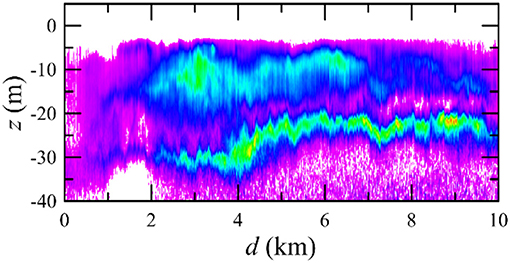
Figure 1. Cross-polarized lidar return from phytoplankton layers in the NE Pacific Ocean as a function of depth, z, and distance along the flight track, d. The color represents the intensity of the lidar signal. Reuse with permission from Churnside and Donaghay (2009).

In a quasi-single-scattering approximation, the depth-dependent signals from the two channels of a polarization lidar are given by Churnside (2008):

$\begin{array}{l}{S}_c(z)=\frac{EAO(z)T_0{T}_s^2\eta v}{2n{(nH+z)}^2}{\beta }_c(\pi ,z)exp\left[-2{\displaystyle {\int }_0^z}\alpha \left(z^{{}^{\prime }}\right)d{z}^{{}^{\prime }}\right]\\ S_x(z)=\frac{EAO(z)T_0{T}_s^2\eta v}{2n{(nH+z)}^2}\left[{\beta }_x(\pi ,z)+2{\beta }_c(\pi ,z){\displaystyle {\int }_0^z}\gamma \left(z^{{}^{\prime }}\right)d{z}^{\prime }\right]\\ exp\left[-2{\displaystyle {\int }_0^z}\alpha \left(z^{{}^{\prime }}\right)d{z}^{{}^{\prime }}\right]& (2)\end{array}$

where S is the lidar signal (photocathode current) for the copolarized or unpolarized (subscript C) and cross-polarized (subscript X) channels and γ is the rate of depolarization of the light by multiple forward scattering. For an airborne system, it is easy to ensure that O(z) = 1 for all depths, leaving four depth-dependent properties of the water (β_C, β_X, α, and γ) to be estimated from these two equations.

Two approaches to retrieval of these parameters from the lidar equations have been considered. The first assumes known relationships between them. For example, the equation for the unpolarized lidar signal can be used to obtain α and β if the ratio of these two quantities can be estimated (Churnside et al., 2014). The second takes advantage of the fact that α and γ are integrated over depth, reducing the effects of small-scale variations. In this approach, an average value for attenuation is obtained and used to produce detailed profiles of scattering (Churnside and Marchbanks, 2015, 2017).

The lidar measurements can often be related to parameters commonly used in ocean color retrievals. For airborne lidar, the lidar-attenuation coefficient is very close to the diffuse-attenuation coefficient, K_d, as long as the laser spot on the surface is large (Gordon, 1982), and this relationship has been verified (Montes et al., 2011; Lee et al., 2013). The most commonly used scattering parameter in ocean color measurements is the particulate backscattering coefficient, b_bp. This can be obtained from the volume scattering function measured by the lidar (Churnside et al., 2017a). The contribution to scattering by seawater is well-known and can be removed. Then, an empirical value for the ratio of b_bp to the volume scattering function at 180° is applied (Churnside et al., 2017a). This approach seems to work better for single-angle measurements at scattering angles near 120° (Boss and Pegau, 2001; Sullivan and Twardowski, 2009; Zhang et al., 2014), and more measurements at 180° are needed.

Since the first recorded detection of fish by airborne lidar in 1976 (Squire and Krumboltz, 1981), a number of studies have shown that lidar compares well with traditional techniques for fish in the upper 30–40 m of the water column (Churnside et al., 2003, 2009, 2017b; Roddewig et al., 2017). The advantage of airborne lidar for fisheries surveys is that it can cover large areas quickly and at lower cost than a surface vessel. On the other hand, these surveys cannot provide the detailed information that can only be obtained through direct sampling from a vessel. The best solution would be aerial surveys coupled with adaptive sampling by surface vessel. Airborne lidar can also be used to document cases of fish avoiding the research vessel performing the survey.

Lidar has also been used to detect zooplankton. The scattering from zooplankton is generally less than that from fish, and detection is more difficult. For copepods, a combination of thresholding and spatial filter is effective (Churnside and Thorne, 2005). A surface layer of euphausiids was detected, but the zooplankton signal in that case could not be separated from the signal produced by the many predators in the layer (Churnside et al., 2011). Unlike most zooplankton, aggregations of jellyfish can produce very large lidar signals, and airborne lidar has been used to describe the internal structure of aggregations of moon jellyfish (Churnside et al., 2016).

There is often a deep chlorophyll maximum near the bottom of the mixed layer in the ocean (Cullen, 1982; Lewis et al., 1983), and the layers of phytoplankton that make up this maximum have been studied by airborne lidar (Vasilkov et al., 2001; Goldin et al., 2007; Churnside and Donaghay, 2009). Often, these layers are very thin (<5 m) and very intense (>3 times the background density) (Durham and Stocker, 2011). These intense layers affect primary productivity, since they are often at a depth that optimizes sunlight and nutrient availability. They also affect transfer of energy to higher trophic levels, since grazing efficiency is high within the layers.

Using phytoplankton as a tracer, several important features of upper ocean dynamics can be measured. The first is the depth of the mixed layer when there is a layer at the pycnocline (Churnside and Donaghay, 2009; Churnside and Marchbanks, 2015). The pycnocline is a density gradient, so it will support propagation of gravity waves, known as internal waves. Internal waves are important in that they transfer significant amounts of heat, energy, and momentum in the ocean (Laurent et al., 2012). Large, non-linear internal waves are particularly interesting, because of their ability to propagate over large distances. They are also particularly amenable to characterization by airborne lidar (Churnside and Ostrovsky, 2005; Churnside et al., 2012). Turbulent mixing of phytoplankton can also be identified by a characteristic power law spectrum of number density. Figure 2 shows a plot of power-spectral density of the cross-polarized lidar return from a constant 10 m depth across Barrow Canyon in the Chukchi Sea west of Utqiaġvik, Alaska. The red line demonstrates the expected K^−5/3 relationship for more than three decades in spatial scale down to the lidar noise level of about 10⁻¹⁹ A² km.

FIGURE 2

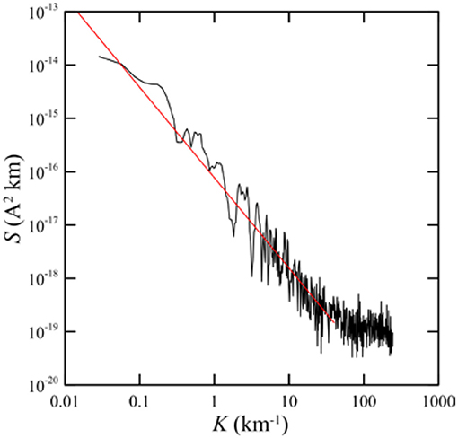
Figure 2. Power spectral density, S, as a function of spatial frequency, K, for the lidar return from a depth of 10 m across Barrow Canyon, Alaska. Red line is the K^−5/3 relationship characteristic of turbulent mixing.

High-Spectral-Resolution Lidar (HSRL)

The HSRL technique is similar to the polarization lidar technique described above and HSRL instruments often include separate co- and cross-polarized detection channels. The differentiating feature is the ability HSRL provides for independent, unambiguous retrieval of attenuation and particulate backscatter without external assumptions (e.g., the assumption of ratio of α to β as described above). The technique has been employed for decades for aerosol and cloud studies (Shipley et al., 1983; Piironen and Eloranta, 1994; Esselborn et al., 2008; Hair et al., 2008), and has only recently been applied to ocean profiling. The most common approach involves a single-frequency (vs. multi-mode) laser transmitter and optical elements in the receiver that spectrally separate molecular backscatter from particulate backscatter. This spectral separation hinges on the fact that backscatter from particles is at the same frequency as the transmitted laser light whereas backscatter from water molecules is shifted by several GHz (e.g., ~7 GHz at 532 nm) due to Brillouin scattering processes. The receiver directs the light, either interferometrically or by other means, to separate detection channels that make range-resolved measurements of backscatter as described in the previous sections. In most implementations of the technique, there are two HSRL channels. One channel predominantly measures molecular backscatter and the other a combination of molecular and particulate backscatter. The profile of attenuation is derived from the derivative (with respect to depth) of the natural logarithm of the molecular channel signal. Particulate backscatter is derived from an algebraic combination of the two channels [see Hostetler et al. (2018) for details]. In addition to independent, accurate retrieval of attenuation and particulate backscatter, another powerful feature of the HSRL technique is the ability to maintain calibration through the entire profile. This is particularly important for higher-altitude airborne (and future spaceborne) implementations for which the intervening atmosphere variably attenuates the received ocean signal due to variations in aerosol and/or cloud optical depth.

Airborne HSRL ocean measurements were first conducted by NASA in 2012 on a deployment based in the Azores, which was conducted as a proof-of-concept study. The instrument used on that study, “HSRL-1,” operated at 532 nm and employed the iodine filter vapor technique for frequency separation in the receiver. Based on that experience, improvements were made to the lidar and it has since acquired data on several airborne deployments, including the Ship-Aircraft Bio-Optical Research (SABOR) mission in 2014 and three deployments for the North Atlantic and Marine Ecosystems Study (NAAMES) in 2015, 2016, and 2017. The HSRL retrievals of b_bp and K_d show excellent agreement with ship-based in-situ estimates made on SABOR (Schulien et al., 2017; Hostetler et al., 2018) and satellite ocean color retrievals (Hair et al., 2016). Data from the HSRL-1 are also used to retrieve estimates of both total and particulate depolarization, and those data along with the b_bp and K_d profiles are currently being assessed for information on community composition. Figure 3 shows aerosol backscatter, aerosol optical depth, b_bp, K_d, and particulate depolarization retrievals from HSRL-1 on 13 May 2016 NAAMES flight in the Western North Atlantic. These data illustrate the ability of the HSRL technique for providing accurate ocean optical properties despite the high and highly variable aerosol optical depth in the overlaying atmosphere.

FIGURE 3

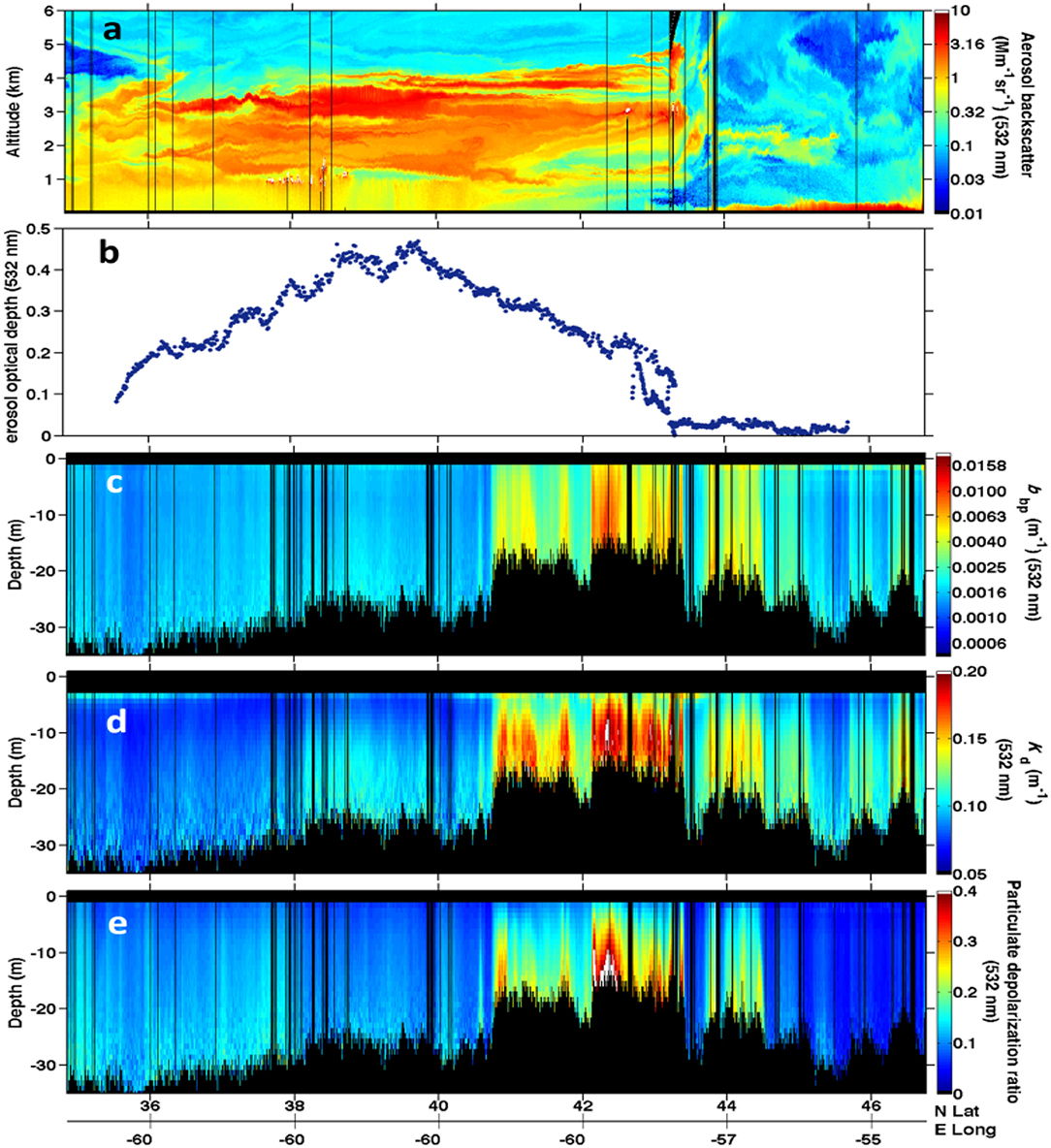
Figure 3. Aerosol backscatter (a), aerosol optical depth (b), b_bp (c), K_d (d), and particulate depolarization (e) retrievals from HSRL-1 on 13 May 2016 NAAMES flight in the Western North Atlantic Modified from Neukermans et al. (2018).

From and engineering perspective, the HSRL technique is much more challenging than the standard backscatter and polarization technique described above. In the receiver, specially designed optical filters are required to spectrally separate molecular and particulate backscatter. In the transmitter, most implementations require a frequency-tunable single-mode laser transmitter, which involves injection-seeding a specially-designed pulse laser with a tunable continuous wave seed laser for precise control of the output wavelength to match the optical filters in the receiver. Concepts do exist that employ multimode laser transmitters; however, these require interferometric receiver filters that must be precisely matched to the characteristics of the laser. Perhaps due to the currently low demand for HSRL instruments and the high cost of the laser and receiver components, commercial lidar vendors have not developed HSRL instruments as a product.

Satellite

While aircraft-flown lidars have provided ocean measurements for decades (see above), the power of satellite-based lidar for ocean biology measurements has been demonstrated only recently (Behrenfeld et al., 2013, 2017; Churnside et al., 2013; Lu et al., 2014; Hostetler et al., 2018). These studies involved analysis of data from the CALIOP instrument on the CALIPSO platform which was designed for atmospheric measurements. It turned out, however, that its 532-nm channels are also sensitive to ocean backscatter. The relatively coarse vertical resolution of CALIOP (30 m in the atmosphere and 23 m in the ocean) and poor detector transient response make vertically resolved ocean retrievals impractical. However, significant scientific impacts have been realized using vertically integrated CALIOP subsurface ocean data. Behrenfeld et al. (2013) used CALIOP data to retrieve particulate backscattering coefficients (b_bp) for the global oceans and, employing published relationships based on b_bp, estimated particulate organic carbon (POC) and phytoplankton biomass, showing that the lidar retrievals were consistent with those obtained with the MODIS spaced-based radiometer.

One (of many) particular strengths of satellite lidar observations is in studying high latitude ocean regions, where ocean color observations from passive radiometers are incomplete (indeed, often completely absent) due to low solar angle and the presence of sea-ice and clouds. Supplying its own light source, CALIOP has already provided an uninterrupted record of plankton stocks for the ice-free portions of the polar oceans. Additionally, being a polar orbiting satellite, the density of retrievals near the poles is superior to that at lower latitudes. Behrenfeld et al. (2017) used a decade of monthly-resolved CALIOP data to demonstrate the processes governing the balance between phytoplankton division and loss rates, thereby advancing a new and evolving understanding of plankton blooms (Behrenfeld, 2010; Behrenfeld and Boss, 2017). An additional finding was that inter-annual anomalies in northern and southern polar-zone plankton stocks were of similar magnitude but driven by different processes. Specifically, growth and loss processes dominated inter-annual variability in the northern polar zone, while variations in plankton stocks of the southern polar zone predominately reflected changes in the extent of ice-free area.

While the atmosphere-focused CALIOP instrument provides valuable ocean data products, it has exceeded its 3-year design lifetime by over 9 years. Significant advances in science capability are envisioned for a follow-on satellite lidar optimized for ocean (as well as atmospheric) retrievals (Hostetler et al., 2018) (Table 1). Several advances are currently possible:

1. Higher vertical resolution: Lidar signals attenuate rapidly with depth, for instance, by a factor of 400 at three optical depths, beyond which the lidar signal is generally not useable due to low signal-to-noise. At CALIOP's 532-nm wavelength, this three-optical-depth limit corresponds to about 50 m in geometric depth in the clearest waters and much less in more turbid waters, which leaves only one or two useable points in the 23-m resolution CALIOP profile. In future space-borne lidars, vertical resolutions of <3 m are achievable with current technology and would enable profiling of vertical structure in backscatter to three optical depths. Such profiling would represent a significant advantage over passive radiometric measurements, for which the measured signals are weighted exponentially toward the ocean surface (with 92% of the signal coming from the first optical depth). Vertically resolved lidar data of phytoplankton biomass, for instance, will reduce errors in estimates of net primary productivity that result from using surface-weighted retrievals to represent ocean properties at greater depths (Platt and Sathyendranath, 1988; Zhai et al., 2012; Hill et al., 2013; Schulien et al., 2017).

2. Higher spatiotemporal resolution: In polar regions, CALIOP or future lidar missions may be used to better document the marginal ice zone composed of a mixture of sea ice and open waters, as well as the frequent open-water fractures found in the ice pack, where phytoplankton growth may be significant and has been hard to capture (see Figure 4). In particular, observations in the leads may be exploited to investigate under-ice phytoplankton dynamics, one of the mysteries of polar environments. Major recommendations in order to achieve this goal would be to increase the spatiotemporal coverage of future lidar missions. This implies reducing footprint diameter and distance between footprints.

3. Independent retrieval of attenuation and backscattering: The standard elastic backscatter lidar technique used for CALIOP cannot separate the backscattered signal from attenuation, so b_bp retrievals in previous publications required either assuming a predictable relationship between backscatter and attenuation or combining CALIOP and passive ocean color data. The former assumptions can introduce significant errors when applied at the local scale. By adding one or more additional channels in the lidar receiver to resolve the optical signal spectrally, the existing HSRL technique enables independent and accurate retrieval of particulate backscatter and attenuation coefficients. The HSRL technique has been used for decades for aerosol measurements (Shipley et al., 1983; Piironen and Eloranta, 1994; Esselborn et al., 2008; Hair et al., 2008), and more recently to retrieve ocean particulate backscatter and the diffuse attenuation coefficient (Hair et al., 2016; Schulien et al., 2017).

4. Addition of other backscattering wavelengths: A future space-borne 532 nm HSRL with high-vertical-resolution capability would enable vertically resolved estimates of phytoplankton biomass, POC, and net primary productivity. Adding HSRL capability at 355 nm in addition to that at 532 would allow independent estimates of algal and CDOM absorption and information on the slope of the particle size distribution.

5. Addition of detectors to measure fluorescence emissions: A further promising direction for application of space-borne lidar is the retrieval of the fluorescence signature of Chl-a and CDOM, which would allow studies of phytoplankton physiology and a better separation of particulate and dissolved pools of organic carbon in the upper ocean. Laser-excited fluorescence from both Chl-a and dissolved organic matter have already been shown to be measurable by airborne lidar instruments in both coastal and open-sea waters (Hoge et al., 1993). Additionally, the ratio of chlorophyll fluorescence and backscattering has been recently found to provide important constraints for the retrieval of phytoplankton functional types (PFT) dominating upper ocean communities. With such data, studies have documented PFT changes through the evolution of the North Atlantic bloom (Cetinić et al., 2015; Lacour et al., 2017).

6. Joint retrievals from combined passive and active sensing: The increase in information obtained with a lidar when combined with that from passive radiometry (with the possibility of polarimetry, e.g., Stamnes et al., 2018b; see section Polarimetry Technique) has been shown to improve estimates of atmospheric aerosols and, consequently, to enhance ocean geophysical retrievals (i.e., through improved atmospheric corrections).

TABLE 1

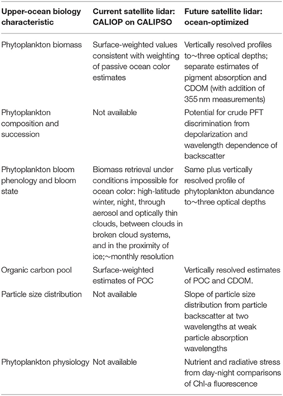
Table 1. Characteristics of upper-ocean biology that can be derived from current and potential future satellite lidar missions Neukermans et al. (2018).

FIGURE 4

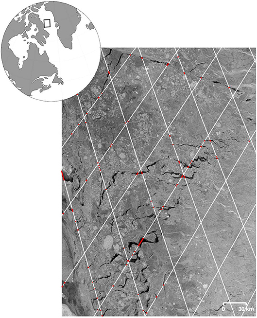
Figure 4. Sentinel 1 SAR (Synthetic Aperture Radar) image on 10th April 2017 in the Baffin Bay (pixel size: 100 × 100 m), showing open-water fractures (black pixels) in the ice pack. White lines depict CALIOP tracks over a 16-day orbit repeat cycle. Red dots indicate where the lidar shots (~100 m footprint; 330 m pulse-to-pulse along-track distance) targeted open-water areas. These represent about 3% of the total shots shown on this image.

It follows from the above that satellite lidar observations are a natural complement to passive radiometric remote sensing. While lidar systems lack the swath width of space-based passive radiometers, the lidar has many sampling capabilities beyond those of passive ocean color. These lidar advantages include (1) measurements independent of solar angle and both day and night, enabling sensing during all seasons at high latitudes and documentation of diel plankton cycles, (2) an ocean-optimized HSRL can provide measurements through aerosol layers of any type (absorbing, as well as non-absorbing) and through optically thin clouds, (3) a lidar's small footprint (e.g., 90 m for CALIOP) enables measurements in gaps between clouds, regardless of cloud shadowing or adjacency effects that can contaminate passive retrievals, as well as sampling through small gaps within and near ice (for CALIOP, the annual coverage is comparable to MODIS at high latitudes, despite its small footprint), and (4) a future lidar with high vertical and spatiotemporal resolution capability would enable the first global three-dimensional view of global ocean plankton ecosystems in conjunction with BGC Argo floats (Johnson and Claustre, 2016).

Polarimetry Technique

Measurement Principle

The overarching goal here is to determine the polarization of light scattered by suspended particles present in either the atmosphere or ocean, as a function of wavelength and scattering angle in order to derive optical properties and infer microphysical information about those particles. Due to the transverse nature of light, a plane electromagnetic wave of light can be modeled as $E=E_0{e}^{i(k•r-\omega t)}$, where E₀ is the complex electric field that propagates along a unit vector k. This propagation direction uniquely determines the meridional plane for a beam of light when combined with the local vertical direction z. The electric field E₀ of the incident light can then be decomposed into parallel ($E_0^{\left|\right|}$) and perpendicular ($E_0^{\perp }$) components with respect to this meridional plane, such that ${\text{E}}_0=E_0^{\left|\right|}+E_0^{\perp }$. For a monochromatic energy flux, it is possible to define the 4 × 1 Stokes column vector I ≡ {I, Q, U, V} using linear combinations of these complex electrical field components as follows:

$\begin{array}{ll}I=\left[\begin{array}{c}I\\ \begin{array}{c}Q\\ \begin{array}{c}U\\ V\end{array}\end{array}\end{array}\right]=c\left[\begin{array}{c}{E}^{\left|\right|}{E}^{|{|}^{\ast }}+E^{\perp }{E}^{{\perp }^{\ast }}\\ \begin{array}{c}{E}^{\left|\right|}{E}^{|{|}^{\ast }}-E^{\perp }{E}^{{\perp }^{\ast }}\\ \begin{array}{c}{E}^{\left|\right|}{E}^{{\perp }^{\ast }}+E^{\perp }{E}^{|{|}^{\ast }}\\ i(E^{\left|\right|}{E}^{{\perp }^{\ast }}-E^{\perp }{E}^{|{|}^{\ast }})\end{array}\end{array}\end{array}\right]& (3)\end{array}$

where c is proportional to the electric permittivity and the magnetic permeability of the medium. The Degree of Polarization can then be defined as: $DoP=\frac{\sqrt{Q^2+U^2+V^2}}{I}$, which spans from 0 when the light is completely unpolarized to 1 when the light is fully polarized. When the circular polarization component, V, is neglected, then the Degree of Linear Polarization is $DoLP=\frac{\sqrt{I^2+U^2}}{I}$. A polarimeter provides Stokes parameters I, Q, U and V by separating and modifying the orthogonal polarized intensities E^∥E^∥* and E^∥⊥E^⊥* of the measured light. The separation and modification can be achieved by passing the light through a polarizing filter and retarder before measurement. It is worth to note that the V component is typically very small at TOA/in the atmosphere and is not measured (or at least not reported) by most polarimeter instruments. The general measurement concept is described by the following equation (Chandrasekhar, 1960; Hansen and Travis, 1974):

$\begin{array}{ll}{I}_m(\chi ,\epsilon )=\frac{1}{2}\left[I_i+Q_{i}cos2\chi +(U_{i}cos\epsilon -V_{i}sin\epsilon )sin2\chi \right]& (4)\end{array}$

where subscript i indicates the Stokes vector elements of the incident light while m indicates the intensity of the measured light, χ is the rotation angle between polarizer axis and the parallel electric field direction and ε is a constant retardation difference between the parallel and perpendicular electrical fields. Thus, the I, Q, and U components can be measured by recording intensities of the measured light with three different orientations of polarizers.

Single Scattering Properties

The Stokes vector defines the polarization state of the incident and measured light. The Mueller matrix is a 4 × 4 transformation matrix describing the scattering process and relating the incident light to the observed light as a function of scattering angle. Thus, the Mueller matrix depends on the properties of the scattering object (i.e., aerosols, hydrosols, or surface). In remote sensing of aerosols and hydrosols, the Mueller matrix is obtained through light scattering theory based on the far-field approximation. Mie scattering refers to light scattering by homogenous spherical particles with a specific complex refractive index and size distribution with particle radii of specific range, which is often used to approximate particle scattering in turbid media. When particles are much smaller in size than the wavelength of incident light, the Mueller matrix can be approximated by the Rayleigh theory of scattering. The scattering by air molecules follows the Rayleigh scattering theory supplemented with a specific depolarization ratio to account for the molecules anisotropy (i.e., molecules do not behave as perfect dipoles) while pure water follows the Einstein-Smoluchowski-Cabannes fluctuation theory of light scattering (Litan, 1968). Also, several numerical approaches have been developed to calculate properties of single scattering of light by larger particles of arbitrary shape and composition such as the T-matrix, Finite Difference Time Domain and Discrete Dipole Approximation (Waterman, 1971; Purcell and Pennypacker, 1973; Yang and Liou, 1996; Mishchenko and Travis, 1998; Yurkin and Hoekstra, 2007). Additionally, inhomogeneous spherical particles can well approximate the backscattering of phytoplankton particles (Robertson-Lain et al., 2014; Moutier et al., 2017; Poulin et al., 2018). In the ocean, due to a lack of knowledge of the shape and composition of hydrosols, spherical particles are typically assumed for RT studies given a refractive index and Junge (power-law) slope for the size distribution. Hydrosol particulates can be separated into organic (phytoplankton) and in-organic (non-algal particles, NAP). Organic particles have a low refractive index relative to the water (n_ph = 1.02~1.08) due to the high water content, while NAPs are more refracting (n_nap = 1.1~1.22) (Aas, 1996; Stramski et al., 2004). The apparent optical effect (i.e., the bulk or mixed Mueller or scattering matrix) is calculated as the relative contribution in scattering of each component. Figure 5 shows the 4 independent elements of the scattering matrix computed from Mie theory for phytoplankton (blue curve) and NAP (red curve), and for mixtures (black curve) based on their scattering coefficient as a weighted average.

FIGURE 5

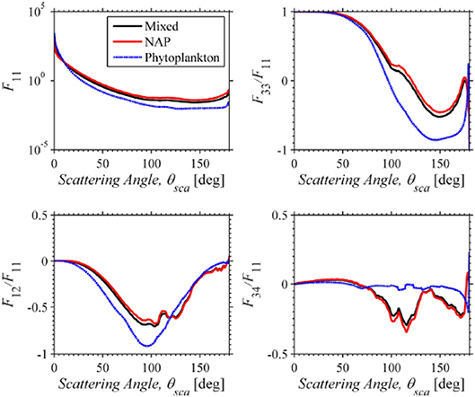
Figure 5. Scattering phase function and normalized polarization elements of the scattering matrix from Mie calculations for one case as an illustration for n_nap = 1.18, n_ph = 1.06, ξ_nap = 4.0, ξ_ph = 4.0, [NAP] = 1.45 g m⁻³, and [Chl] = 10.5 mg m⁻³ at 440 nm. Reuse with permission from Ibrahim et al. (2012).

Figure 5 shows the phase function and the normalized polarization components of the Mie scattering elements (F₁₁, F₁₂/F₁₁, F₃₃/F₁₁, and F₃₄/F₁₁) for one case of chlorophyll and NAP concentrations and for one case of Junge Particle Size Distribution (PSD) slope (ξ_nap = ξ_ph = 4), as an illustration. The matrix is calculated for spherical particles. The polarization elements (F₁₂/F₁₁, F₃₃/F₁₁, and F₃₄/F₁₁) of the scattering matrix of phytoplankton particles are similar to those obtained for Rayleigh scattering, because the relative refractive index is very low, i.e., 1.06, similar to what was presented in Figure 4 of Gilerson et al. (2013). In contrast, the shape of the polarized scattering matrix elements of NAPs are significantly different, due to their high refractive index, with exception of the near forward and backward direction where it exhibits a weak polarization effect according to Mie-Lorenz theory. The figure shows the strong separability of the two types of particles when using the polarized components of the scattering matrix, as opposed to the F₁₁ element only.

The Utility of Polarimetry in Ocean Remote Sensing

Inherent Optical Properties

Beam attenuation coefficient

The particulate attenuation coefficient, c_p, of hydrosols co-varies with the particulate organic carbon concentration (POC) as well as with the phytoplankton carbon biomass (Loisel and Morel, 1998; Behrenfeld and Boss, 2003; Behrenfeld et al., 2005; Cetinić et al., 2012; Graff et al., 2015; Werdell et al., 2018). Several studies suggest that there is a first-order relationship between the ratio of c_p to chlorophyll concentration (c_p:Chl), which may be used as an index of phytoplankton carbon (C) biomass to chlorophyll concentration ratio (C:Chl) and phytoplankton physiology, which is important for estimating primary production of the oceans. Thus, retrieval of the attenuation coefficient from remote sensing would allow for a drastically better understanding of the carbon cycle on the global scale, which is a primary goal of many ocean color satellite missions.

Ibrahim et al. (2012, 2016) have shown that there is a direct relationship between the attenuation to absorption ratio and the Degree of Linear Polarization (DoLP; which is given by setting V = 0 in the definition of DoP) just beneath the ocean surface at three wavelengths in the visible and for a wide range of viewing geometries. The relationship shown in top row of Figure 6 is based on VRT simulations for a large dynamic range of coastal water IOPs (Ibrahim et al., 2016). This relationship was confirmed with in-water observations showing the possibility of retrieving the attenuation coefficient of hydrosols as shown in the lower row of Figure 6. These results are also consistent with the theoretical analysis of Chami and Defoin Platel (2007) based on RT modeling. In addition, Tonizzo et al. (2009) also illustrated the sensitivity of DoLP to variations in water types. Based on in-water observations, clear waters show high DoLP values in the blue and green wavelengths, while the opposite occurs for the more productive water. Adding CDOM in the more turbid water increases the DoLP in the blue even more, due to the decreased number of scattering events.

FIGURE 6

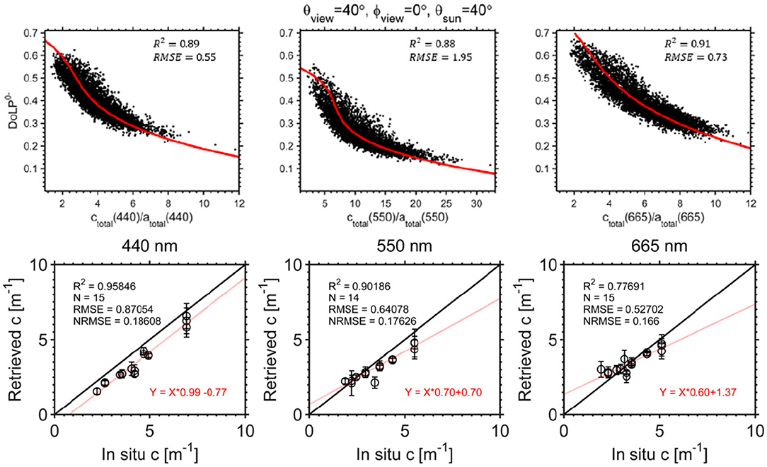
Figure 6. The upper row shows the simulated DoLP just beneath the ocean surface vs. the ratio of the attenuation to absorption coefficients for three wavelengths in the visible wavelengths at one specific geometry and for a wide range of coastal ocean IOPs. The lower row is the validation based on in-water polarimeter observations and in-water beam attenuation coefficient measurements from WETLabs ac-s. Reuse with permission from Ibrahim et al. (2016).

Particle sizes and complex refractive index

Oceanic hydrosols such as plankton and mineral particles vary in size and composition. Traditionally, the PSD is retrieved from the spectral slope of the backscattering coefficient, which can be derived from spaceborne radiometers by assuming the power law (Junge) size distribution for spherical particles (Loisel et al., 2006; Kostadinov et al., 2009). Laser diffraction measurements of the particle size distribution in different oceanic regions showed that the size distribution of marine particles can be approximated by the Junge-like power law except in cases where there is are rapid changes in a phytoplankton species population (Buonassissi and Dierssen, 2010; Reynolds et al., 2010, 2016).

Organic particles have low refractive index and thus are less effective scatterers, while inorganic hydrosols such as sediments have a high refractive index, implying that they are more efficient scatters that tend to depolarize the light. In coastal waters, the DoLP is generally smaller than in the open ocean due to the high amount of sediments with a high bulk refractive index.

In Figure 7, Loisel et al. (2008) showed DoLP for various scattering angles for low and high refractive index particles. The molecular scattering exhibits very strong polarization at 90° scattering angle, decreasing when moving to smaller/larger angles. When particles are added, the position of the peak of polarization, as well as its intensity, changes on particle size, refractive index, and concentration. For large particles, the DoLP decreases strongly. For this reason, the measurement of DoLP provides information on the relative proportion between small and large particle sizes in the observed field. Multiple scattering and scattering by non-spherical particles also tend to lower the DoLP (Ivanoff et al., 1961). Tonizzo et al. (2011) have shown retrievals of hydrosols microphysical properties using a recursive fitting of the in-situ DoLP measurements with RT simulations. For remote sensing applications, Ibrahim et al. (2016) suggested to estimate the bulk refractive index using the CDOM corrected spectral attenuation coefficient to approximate the Junge PSD, derive the backscattering ratio from the backscattering and total scattering coefficient and apply the method of Twardowski et al. (2001) based on the Mie theory.

FIGURE 7

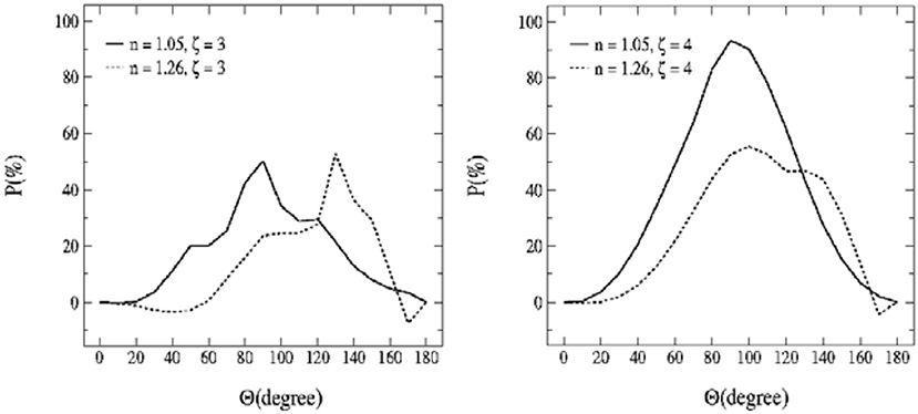
Figure 7. The DoLP (%) [labeled as P(%)] in-water as a function of scattering angle for four different polydisperse assemblages of hydrosols: size distributions with the Junge PSD slope ξ = 3 (left) and ξ = 4 (right) and particles with low refractive index (organic particles n = 1.05) and high refractive index (in-organic particles n = 1.26). Reuse with permission from Loisel et al. (2008).

Improved net-primary productivity (Npp)

In complex waters, the separation between the optical contributions of different ocean constituents becomes more challenging. The ambiguity in the inverse problem using scalar radiance is too high. Thus, the estimate of primary productivity can be biased in these water conditions. Polarimetry potentially allows the separation of organic and in-organic contributions, which in-turn allows improved NPP estimates. Chami and McKee (2007) suggest that it is possible to retrieve the suspended particulate matter (SPM) from DoLP measurements at the Brewster angle. Using theoretical modeling they showed that an empirically based inversion approach could retrieve the concentration of inorganic particles from underwater polarized radiance measurements regardless of the phytoplankton content in coastal waters.

Turbidity

Chami et al. (2001) and Chami and McKee (2007) have shown that it is possible to retrieve the turbidity in complex waters using the polarized reflectance through a RT sensitivity analysis. It is possible to discriminate the sediment concentration from the phytoplankton using the polarized signal at the red wavelength. The polarized reflectance shows an enhanced sensitivity to in-water sediments and their microphysical properties, as compared to the remote sensing reflectance (Rrs). Chami and McKee (2007) showed the potential of the degree of polarization measurements at the Brewster angle in the specular direction to retrieve the concentration of sediment particles. Ibrahim et al. (2016) corroborated some of these results in a recent study.

Enhanced Atmospheric Correction

Improved aerosol characterization

Improved aerosol characterization will improve atmospheric correction and thus directly benefit ocean color remote sensing. There is a strong heritage within the atmospheric community of using multi-angular polarimeters for aerosol characterization, beginning with POLDER (Deuzé et al., 2000; Hasekamp and Landgraf, 2005; Dubovik et al., 2011; Hasekamp et al., 2011, 2019; Tanré et al., 2011). This heritage and further studies have shown that multi-angle polarimetry advances aerosol characterization beyond the capabilities that single-view total radiation measurements can achieve in terms of number of microphysical characteristics retrieved (Chowdhary et al., 2001, 2002, 2005; Waquet et al., 2009, 2013; Harmel and Chami, 2011; Knobelspiesse et al., 2012; Ottaviani et al., 2013; Peers et al., 2015; Xu et al., 2016, 2017; Gao et al., 2018; Stamnes et al., 2018a).

Improved glint correction

He et al. (2014) provide evidence of the advantages of including polarimetry for atmospheric correction over the ocean. They describe a method for retrieving the normalized water-leaving radiance (L_wn), using the parallel polarized radiance (PPR = I + Q), where I and Q are the first two components of the Stokes vector I. Their results, both from simulations and from application to POLDER data, demonstrate that use of PPR provides two important enhancements to ocean color retrieval. First, it reduces the sun glint at moderate to high solar zenith angles. Second, it boosts the ocean color signal relative to the total radiance received by satellite sensors at large view zenith angles. These advantages are explained by the compensating effect between the total radiance and the polarization. For example, as the view zenith angle increases, because of the longer path length through the atmosphere, the total radiance received by the satellite increases, causing the relative ocean color signal reaching the satellite to decrease. Meanwhile, the magnitude of Q increases with path length, but in the negative sense, which offsets the increase in I, and slows down the increase in PPR with path length through the atmosphere. Harmel and Chami (2013) have also shown that a better characterization of the glint signal is obtained using multi-angular polarimetric measurements from the PARASOL sensor. One may also consider using unpolarized reflectance instead of total reflectance to retrieve water properties, as suggested by Frouin et al. (1994) and Krotkov et al. (1992). The contribution of the water body to the TOA signal is generally enhanced using this component, except over optically thick atmospheres (due to multiple scattering), making the atmospheric correction easier. Sun glint using this method is mitigated and using polarization information in addition to spectral information in the near infrared and shortwave infrared facilitates determination of the aerosol model necessary for the atmospheric correction (Foster and Gilerson, 2016).

Turbid water atmospheric correction

Zhai et al. (2017) showed that in scattering coastal waters, the polarized reflectance at the TOA in the NIR bands is less significant than the scalar radiance, thus enabling improved separation of aerosol and ocean contributions to the observed signal. The growing interest in IOPs in the UV poses a new challenge for atmospheric correction because of the confounding effects of absorption by aerosols, and specifically lofted smoke or dust layers. Collocated lidar and polarimetry can help to unravel the in-water and in-air contributions but, if not available, emerging passive techniques based on spectral and/or multi-angle observations in the O₂ A-band (~765 nm) can be used (Davis and Kalashnikova, 2018, and references therein).

Simultaneous retrieval of aerosol and water-leaving radiance

Several simultaneous retrieval algorithms have been developed using multi-angle polarization measurements, where the aerosol properties and the water-leaving radiance are retrieved simultaneously. Chowdhary et al. (2005) developed a joint retrieval algorithm using the RSP data that retrieved the aerosol properties and water optical properties with a bio-optical model parameterized by chlorophyll concentration. Hasekamp et al. (2011) developed a retrieval algorithm using measurements from PARASOL with a bimodal aerosol model and an ocean model parameterized by chlorophyll concentration, wind speed and direction, and foam coverage. Xu et al. (2016) developed a retrieval algorithm using the AirMSPI dataset with a multi-pixel smoothing constraint and a simplified bio-optical model. Gao et al. (2018) developed a simultaneous retrieval algorithm for coastal waters using a bio-optical model including contributions from phytoplankton, CDOM, and non-algal particles. Stamnes et al. (2018b) developed a retrieval framework that can combine lidar and polarimeter measurements (HSRL+RSP) in the coupled atmosphere-ocean system to simultaneously retrieve the aerosol microphysical and ocean properties.

Challenges in Polarimetric Ocean Remote Sensing

Vector Radiative Transfer Models

Bio-optical model

Traditionally, the ocean color community has relied mostly on scalar radiative transfer codes such as Hydrolight for remote sensing purposes (Mobley, 1994). However, Hydrolight lacks the ability to simulate a polarized light field in the ocean, and therefore cannot support the development of new remote sensing methods that will make use of polarization measurements. VRT codes that do simulate the polarized field require better representation of aerosol and hydrosol optical properties, including incorporation of the full 4 × 4 single scattering matrix of particle properties into the VRT code. It is therefore necessary in order to have a physically consistent scattering matrix to specify the PSD, complex refractive index, and shape and apply one of several single scattering methods such as Mie (spherical), T-matrix (elliptical), Discrete Dipole Approximation, or geometric optics to calculate the scattering matrix. In terms of hydrosols, there is a significant lack of observational information to constrain particle characteristics, especially morphology, in order to specify particle microphysical properties and calculate the intrinsic particle scattering properties. The specification of particle properties therefore introduces uncertainty into VRT attempts to simulate the polarized light field. Additionally, a full coupling between single scattering properties and bulk IOPs is necessary, and yet are not mapped out.

Fully coupled AO RT models

The ultimate goal of ocean color (scalar and/or polarimetric) measurements is to obtain information about the “health” of its biogenic constituents. For this purpose, access to accurate RT models of the coupled AO system is of paramount importance. To interpret polarimetric measurements, reliable, accurate, and efficient modeling of the polarized radiation represented by the Stokes vector in open oceanic regions as well as turbid coastal areas is required. For example, as reviewed by Stamnes et al. (2018a), such modeling is needed to develop forward-inverse methods required to quantify types and concentrations of aerosol and cloud particles in the atmosphere, as well as dissolved organic and particulate biogeochemical matter in lakes, rivers, coastal and open-ocean water, and to simulate the performance of remote sensing detectors deployed in space. For example, machine learning techniques for accurate cloud screening and retrieval of aerosol and water IOPs in complex AO systems can be based on extensive RT simulations of the coupled AO system (Fan et al., 2017; Chen et al., 2018). Polarized VRT simulations of the coupled AO system can also be used in conjunction with inverse modeling to retrieve the IOPs and vertical location of absorbing atmospheric aerosols as discussed by Stamnes et al. (2018a). Coupled VRT simulations are also required for accurate simultaneous retrieval of aerosol and ocean properties using polarimeter data (Xu et al., 2016; Stamnes et al., 2018b). Such models exist and employ various methods to solve the RT equation, for example adding and doubling (de Haan et al., 1987; Chowdhary et al., 2006; Xu et al., 2016), successive-order-of-scattering (Zhai et al., 2010; Chami et al., 2015), matrix operator (Ota et al., 2010), and Monte Carlo (Ramon et al., 2019). Research frontiers on RT modeling in coupled ocean-atmosphere systems are discussed in great details in Chowdhary et al. (2019). For applications at high latitudes, the curvature of the Earth should be accounted for in the RT simulations (Ding and Gordon, 1995; He et al., 2018), and for analysis of airborne polarimeter data coupled RT simulations are also required (Xu et al., 2016; Stamnes et al., 2018b).

In-elastic scattering VRT

Inelastic scattering in ocean waters includes Raman scattering, Fluorescence by Colored Dissolved Organic Matter (FDOM), and fluorescence by phytoplankton as a by-product of photosynthesis. Scalar solutions of the radiation field have been published with the capability of modeling these effects (Mobley, 1994; Schroeder et al., 2003). In this new era of remote sensing using polarized signals, it is important to have an accurate radiative transfer model that can couple the effect of polarization, flexible atmosphere, and ocean optical properties, and both elastic and inelastic scattering effects. Zhai et al. (2017) have developed a vector radiative transfer model that uniquely combines all these features. Later Zhai et al. (2018) further incorporated photochemical and non-photochemical quenching effects in the solution, which can model fluorescence quantum yield as a function of photosynthetic available radiation. This new radiative transfer package will be an important tool for exploring information content in hyperspectral and polarimetric measurements of ocean constituents.

Multi-angular limitation

Snell's cone due to surface refraction limits the angular information from beneath the ocean surface as shown in Figure 8. A large range of the angular information below the surface is not transmitted to above the surface due to the total internal reflection. Thus, the application of algorithms that utilize the angular distribution of ocean upwelling light, could be limited, however further analysis is required.

FIGURE 8

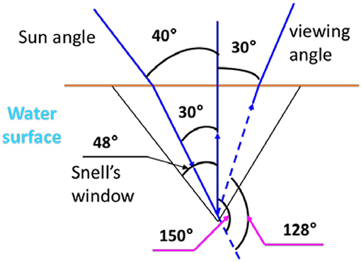
Figure 8. Air-sea interface showing the refraction of the light from below to above the ocean. The solid black lines show the limits of the Snell window.

Instrumentation

Characterize hydrosol scattering matrix, size distribution, and refractive index

So far there are very few measurements of the microphysical properties of hydrosols such as the refractive index and the scattering matrix. Voss and Fry (1984) attempted to measure the scattering matrix of hydrosols in the open ocean. Their measured scattering matrix in clear water conditions showed that the elements of the scattering matrix does not follow the Rayleigh scattering pattern, although there are similarities. All the off-diagonal elements, except F₁₂ and F₂₁ are zeros due to a slight particle anisotropy of orientation preference. Their conclusion is that Mie scattering cannot reproduce the measured scattering matrix due to the limitations of sphericity assumption. Volten et al. (1998) realized laboratory measurements of F₁₁ and F₁₂ for phytoplankton cultures signifying that Mie scattering cannot approximate scattering by phytoplankton particles. Follow-up in-situ measurements of the scattering matrix in clear waters, and for different types of turbid waters including sediment-laden and phytoplankton dominated waters, will be critically relevant to assessing and improving retrievals using polarimeter and hyperspectral remote sensors, such as NASA's PACE mission. And, measurements of the phase function near or at 180 degrees will be important for improving understanding of current and future lidar ocean measurements. Current in-situ commercial instruments, such as the WETLabs MASCOT and LISST-VSF, which measures F₁₁ and F₁₂ of the scattering matrix, will provide additional insight into the hydrosol microphysical properties in conjunction with PSD instruments such as the Sequoia Scientific LISST (Karp-Boss et al., 2007; Sullivan and Twardowski, 2009; You et al., 2011; Gilerson et al., 2013).

In-situ polarimetric instruments

Table 2 shows potential in-situ polarimetric instruments that can be deployed either in- or just above-water which can be used to develop and validate algorithms:

TABLE 2

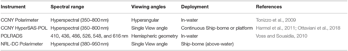
Table 2. List of in-situ polarimeters for ocean applications.

Airborne polarimeters

Airborne polarimeters have been used for numerous field campaigns aimed at studying aerosols and clouds. Some of these instruments could be used to develop remote sensing algorithms for IOP retrievals. Table 3 provides some of these instruments.

TABLE 3

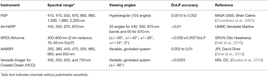
Table 3. List of Multi-angular airborne polarimeters that can be used to develop and test algorithms.

Previous, Current, and Future Missions

Previous and current ocean color missions sponsored by various space agencies (see illustrative example in Figure 9) have focused on utilizing the spectral information at one viewing geometry. Examples include SeaWiFS, MODIS-Aqua/Terra, SNPP-VIIRS, MERIS, Sentinel-3, and GOCI. Multi-angle satellite instruments such as MISR-Terra have been used extensively for aerosol characterization by utilizing the angular distribution of scattered light to distinguish the aerosol properties, however the instrument only measures total (intensity) scattered radiation and is missing the polarization signal. JAXA's SGLI onboard GCOM-C is a single-view instrument that measures the polarized light at two spectral channels in the red and NIR wavelengths. Multi-angle polarimetric information, however, is crucial for retrieving properties about the Atmospheric-Oceanic (AO) system. While there may be some limited capability for SGLI's polarized channels for retrieving ocean properties, SGLI is expected to help quantify the surface glint contribution, which is highly polarizing.

FIGURE 9

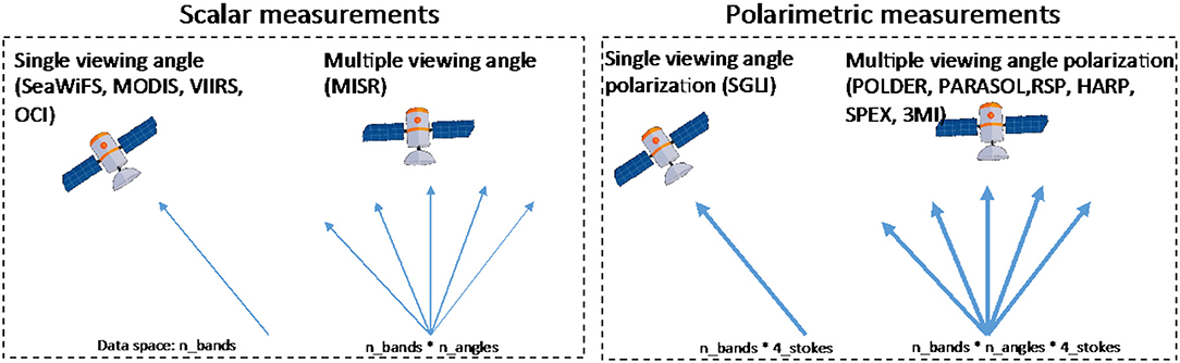
Figure 9. Observing system configurations of scalar and polarimetric measurements at single and multiple viewing geometries. The data space indicates the increased dimension of multi-angular polarimeters from single view radiometers as a proxy to the information content of the measurements.

Space-borne multi-angle polarimeters such as CNES POLDER/PARASOL have been successful in characterizing aerosol and cloud optical and microphysical properties. There are very few studies examining the utility of POLDER/PARASOL for ocean remote sensing applications. In fact, only one study by Loisel et al. (2008) has shown the potential of using the DoLP to distinguish hydrosols' microphysical properties from POLDER. In Figure 10, the radiative transfer simulations, performed for different polydisperse assemblages of suspended marine particles showed that there is an hyperbolic trend between R_rs and the DoLP. The scatter of the POLDER data observed around the hyperbolic trend may be explained by changes in the bulk particulate assemblage.

FIGURE 10

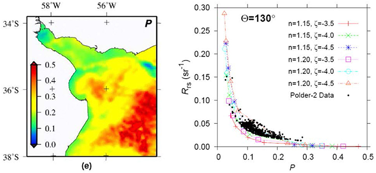
Figure 10. POLDER retrieval of the DoLP shown in the left-hand side figure over complex coastal waters (Rio de la Plata estuary). The right-hand side shows the relationship, obtained from radiative transfer simulations, between the DoLP (shown as “P” on the x-axis) and the R_rs for different hydrosol microphysical properties. The black dots show observed data points overlaid the theoretical relationship. Reuse with permission from Loisel et al. (2008).

In the next few years we expect the launch of new space-borne polarimeters. NASA's PACE mission will host two advanced polarimeters, HARP2 and SPEXone. HARP2 is a hyperangular polarimeters that measures light at 3 visible and 1 NIR channel. The instrument is designed for cloud remote sensing and is expected to significantly benefit aerosol remote sensing. SPEXone is a hyperspectral polarimeter that monitors the spectral range 385–770 nm continuously (resolution 2–5 nm for radiance and 15–40 for DoLP) at five viewing angles. The instrument is designed specifically for aerosol remote sensing (Hasekamp et al., 2019). Another NASA mission expected in the same time frame as PACE is MAIA, which will include a multiangle polarimeter with nadir spatial resolution of 200 m and the ability to point at specific targets. However, MAIA's science objectives are public health, and therefore will be targeting land-based population centers and will not obtain global coverage. In addition to the new NASA missions, ESA is planning to launch 3MI which is a follow-on instrument of POLDER, but with added spectral capability that will enhance its ability to characterize aerosol and cloud properties (Fougnie et al., 2018). While these planned sensors will aid ocean color retrievals indirectly by better characterizing aerosols and improving atmospheric correction, none of these sensors are designed for direct ocean color applications for the following reasons:

1) Coarse spatial resolution (3–4 km).

2) Non-pointing instruments, which leads to measurements in viewing plane that could be contaminated by glint. Aerosol and cloud polarimetry prefer principal plane measurements to maximize the range of scattering angles, however ocean polarimetry needs to measure the light at an off-principal viewing plane to reduce glint, while still being not be too far from the principal plane in order to maximize the polarized signal (i.e., azimuth angle = 30 to 60°). This preference means that ocean coverage would be reduced.

For ocean applications, the radiometric accuracy of the instrument should be very high to enable the detection of small-scale variations of the polarized light in the ocean. For example, Ottaviani et al. (2018) have shown that based on RT simulations, it is possible to detect the polarized ocean reflectance using sensors better than 8.5 × 10⁻⁴ in polarimetric accuracy. Detecting variability in DoP due to changes in the IOPs from space observations is more attainable than the polarized reflectance due to the fact that DoP is a ratio that primarily depends on the random noise of the detector. Meanwhile the polarized reflectance is more sensitive to the systematic uncertainty of the sensor that can be more significant than the random noise term, however it depends on the instrument design. Although, there are no studies on the requirements of ocean polarimeters, in-terms of detection uncertainties, SPEXone on-board the planned PACE mission is expected to be utilized for ocean applications due to its high polarimetric accuracy (see Table 3), however limited in the spatial resolution. State of the art sensors, with improved polarization detection capability designed for ocean color applications are needed.

Outreach and Education

The aim of this section is to provide some suggestions to better connect scientist with end-users in the domain of polarimetry and lidar technologies. End-users include peers, not necessarily in the same field of work, funding organizations, decision makers, and the general public. All of them have a role to play in planning and implementing ocean observation and monitoring. Polarimetry and lidar technologies have a great potential in filling gaps in societal and scientific knowledge needs. But improvements in technologies access, data management, accessibility and dissemination are clearly needed.

No in-situ or airborne oceanic profiling lidar are currently commercially available. The current oceanic profiling lidar are developed in laboratories. For most laboratories, the task of developing their own in-situ or airborne lidar is intensively labor and cost consuming that will prevent short-term efforts for the dissemination of these instruments. This can only be done in conjunction with small and medium enterprises (SMEs). Because of the size of the market, public funding will be necessary to start the collaboration with the SMEs. Without any easy access to in-situ oceanic profiling lidar, the technique will not be fully accepted by the ocean color community and no advance in science will occur.

All the data should be open access, with standardized file format and metadata. A dedicated website should provide relevant and easy-to-use distribution tools, with near real time data visualization. A section on data product description and documentations with simple infographics on the methods of measurement are vital to target a large audience. And finally, an interactive platform where scientists and end-users can exchange ideas, give feedbacks, ask for specific needs, would be very appropriate.

In term of education, to our knowledge, the lidar and polarimetry techniques are not included in Master programs for Ocean Optics and related fields. In order to increase awareness of oceanic profiling lidar, the theory and practical use of the instrument must be included in their curriculum. The same should also occur during summer schools, such as the one organized by the University of Maine or the one organized by the International Ocean Color Coordinating Group. These Summer Schools are attended by Msc/PhD students and early career scientists working on ocean color. If we want future scientists in the field to tackle the use of lidar and polarimetry techniques, we need to include classes on these topics during these summer schools.

Conclusion and Perspectives

Passive radiometric space-borne observations of the ocean color allow for the estimation of the optical properties and concentration of the marine particles, weighted- over the first meters near the surface of the ocean. These observations are available on a 2+-day global coverage basis for the past 20 years. It is now time to go beyond these observations to get access to (1) the profiles of these parameters through the first 3 optical depths and (2) information about the shape and concentration of these marine particles. To do that, the ocean color community must use other observational techniques that have been widely used for the study of the aerosols and clouds: Lidar and polarimetry.

While these techniques have sporadically been used for ocean studies inr the past 30 years, they did not get as much as attention in the ocean community as in the aerosol/clouds community for various reasons (including the unavailability of in-situ and space-borne instruments dedicated to the ocean). With new instruments (in-situ and potentially, spaceborne), the time is for the ocean color community to embrace the scientific potential of these techniques. To make it possible for the community to more thoroughly exploit the science benefits of these techniques, we recommend the following steps be taken:.

Ocean Lidar Recommendations

- Development of compact, cheap and easy to deploy elastic backscatter and HSRL lidar for shipborne and airborne ocean-profiling applications. The ocean-profiling lidars are currently limited to one-off instruments and are not commercially available. Recent technological advances in lasers and detectors show promise for reducing the size, power, and cost of ocean profiling lidars. Collaboration with small and medium companies is necessary to take advantage of these technologies and make these instruments available to research laboratories for deployment on field campaigns.

- Development of a spaceborne HSRL with 355 and 532 nm wavelengths and a fluorescence sensor at 684 nm. The current CALIOP lidar instrument on-board the CALIPSO satellite has a coarse vertical resolution that prevents acquisition of useful depth-resolved information. A future space mission should have a vertical resolution of 3 meters or less. Ideally, this spaceborne lidar should flown in an orbit synergistic with those of future ocean color instruments.

- Development of radiative transfer code to simulate the laser path for diverse oceanic water types. Studies on the lidar waveform are necessary for understanding the impact of the concentrations of marine particles on the shape and intensity of the lidar signal.

Ocean Polarimetry Recommendations

- Radiative transfer codes are as good as their inputs. In order to understand the theoretical framework of polarimetry in the ocean a suite of instruments need to be developed to better characterize the input to radiative transfer. Due to the lack of understanding hydrosols morphology and composition, instruments that measure their microphysical properties (particle size distribution, shape, internal structure, refractive indices of their internal components) and/or their full (4 × 4) scattering matrices are necessary to close this knowledge gap.

- Development of in-situ polarimeters, including those with hyperangular measurements, and hyperspectral capabilities from the UV to NIR. These instruments should be deployed in various water conditions to capture a large dynamic range of IOPs to allow for the development and validation algorithms.

- Investment in more field campaigns that include both in-situ and airborne polarimetry. These field campaigns should focus on ocean applications in scientifically interesting water and atmospheric conditions (i.e., in plankton bloom, coastal waters, and in the presence of absorbing aerosols) of which polarimetry can significantly contribute.

- Development of a spaceborne multi-angular polarimetric sensors designed for ocean applications. Pointing (gimbled) sensors are ideal for geometry targeting with high spatial resolution (1 km or better). The polarimetric accuracy should be high enough (better than 1% and highly preferably better than 0.5%) to capture the small polarized signal emerging from the ocean at the top of atmosphere.

- Development of the polarimetry atmospheric correction algorithms. These algorithms should have the capacity to retrieve both the intensity I and the polarization components (Q, U, and V) from the satellite measured Stokes vector.

Common Recommendations

- Ideally, the ocean polarimeter and ocean lidar airborne field campaigns should be coordinated together, and including hyperspectral spectroradiometer ocean color measurements in the VIS and UV. It may be beneficial to calibrate the airborne/oceanic polarimeter and hyperspectral (VIS and UV) instruments together in the lab, prior to and immediately after the field campaign studies are conducted.

- It is also recommended to provide training and education materials to students and early career scientists on ocean lidar and polarimeter techniques through the development of new courses in Masters and Summer School curricula. These courses will increase the exposure of these two important topics and will increase interest in the ocean optics community to produce novel research ideas.

Author Contributions

CJ and AI coordinated the manuscript and wrote the introduction and conclusion. Jchu provided sub-section on Airborne Lidar. CJ, FA, DD, SV, ER, and IS contributed to sub-section In-situ Lidar. CH contributed to sub-sections High-Spectral-Resolution-Lidar and Lidar Satellite. EB, MJB, LL, and MB provided sub-section Lidar Satellite. LL and CJ contributed to section Outreach and Education. AI provided section Polarimetry Technique with the contribution of sub-sections Particle sizes and complex refractive index by LD-G, HL, and EB, sub-section Improved Glint Correction by LR and RF, sub-section Simultaneous Retrieval of Aerosol and Water-Leaving Radiance by MG, sub-section Fully Coupled AO RT Models by KS and SS, and sub-section In-Elastic Scattering VRT by P-WZ. KK provided Table 3. BC and JCho provided parts of section Measurement Principle. SS contributed to the introduction, sections Measurement Principle, Fully Coupled AO RT Models, Previous, Current and Future Missions, and the conclusion. BF, DG, OH, JCho, LR, KS, SS, ZA, JW, AD, OK, VM, XH, and P-WZ contributed revisions throughout section Polarimetry Technique.

Conflict of Interest Statement

The authors declare that the research was conducted in the absence of any commercial or financial relationships that could be construed as a potential conflict of interest.

The handling editor declared a shared affiliation, though no other collaboration, with one of the authors OK at time of review.

Acknowledgments

Portions of this work were performed at the Jet Propulsion Laboratory, California Institute of Technology, under a contract with the National Aeronautics and Space Administration. The JPL work was supported by the PACE science team grant, under Paula Bontempi. NASA, CNES, and ESA are acknowledgments for the access to the CALIPSO and Sentinel-1 images. CNES through the TOSCA program is acknowledged for funding the publication.

References

Aas, E. (1996). Refractive index of phytoplankton derived from its metabolite composition. J. Plank. Res. 18, 2223–2249. doi: 10.1093/plankt/18.12.2223

CrossRef Full Text | Google Scholar

Abdallah, H., Baillet, J.-S., Baghdadi, N. N., Saint-Geours, N., and Fabre, F. (2013). Potential of space-borne LiDAR sensors for global bathymetry in coastal and inland waters. IEEE J. Selec. Topics Appl. Earth Obs. Remote Sens. 6, 202–216. doi: 10.1109/JSTARS.2012.2209864

CrossRef Full Text | Google Scholar

Adams, J. T., Aas, E., Højerslev, N. K., and Lundgren, B. (2002). Comparison of radiance and polarization values observed in the mediterranean sea and simulated in a monte carlo model. Appl. Opt. 41, 2724–2733. doi: 10.1364/AO.41.002724

PubMed Abstract | CrossRef Full Text | Google Scholar

Ahmad, Z., and Fraser, R. S. (1982). An iterative radiative transfer code for ocean-atmosphere systems. J. Atmos. Sci. 39, 656–65. doi: 10.1175/1520-0469(1982)039<0656:AIRTCF>2.0.CO;2

CrossRef Full Text | Google Scholar

Aibulatov, N. A., Zavialov, P. O., and Pelevin, V. V. (2008). Features of hydrophysical purification Russian Black Sea coastal area near the mouths of rivers. Geoecology 4, 301–310.

Babichenko, S., Poryvkina, L., Rebane, O., and Sobolev, I. (2016). Compact HLIF LiDAR for marine applications. Inter. J. Remote Sens. 37, 3924–3937. doi: 10.1080/01431161.2016.1204479

CrossRef Full Text | Google Scholar

Bailly, J. S., Le Coarer, Y., Languille, P., Stigermark, C. J., and Allouis, T. (2010). Geostatistical estimation sof bathymetric LiDAR errors on rivers. Earth Surf. Process Landforms 35, 1199–1210. doi: 10.1002/esp.1991

CrossRef Full Text | Google Scholar

Barbini, R., Colao, F., Fantoni, R., Palucci, A., and Ribezzo, S. (1999). Shipborne laser remote sensing of the Venice lagoon. Int. J. Remote Sens. 20, 2405–2421. doi: 10.1080/014311699212092

CrossRef Full Text | Google Scholar

Behrenfeld, M. J. (2010). Abandoning sverdrup's critical depth hypothesis on phytoplankton blooms. Ecology 91, 977–989. doi: 10.1890/09-1207.1

PubMed Abstract | CrossRef Full Text | Google Scholar

Behrenfeld, M. J., and Boss, E. (2003). The beam attenuation to chlorophyll ratio: an optical index of phytoplankton physiology in the surface ocean?. Deep Sea Res. 50, 1537–1549. doi: 10.1016/j.dsr.2003.09.002

CrossRef Full Text | Google Scholar

Behrenfeld, M. J., Boss, E., Siegel, D. A., and Shea, D. M. (2005). Carbon-based ocean productivity and phytoplankton physiology from space. Flobal. Biogeo. Cycles 19:2299. doi: 10.1029/2004GB002299

CrossRef Full Text | Google Scholar

Behrenfeld, M. J., and Boss, E. S. (2017). Student's tutorial on bloom hypotheses in the context of phytoplankton annual cycles. Global Change Bio. 13858, 1–23 doi: 10.1111/gcb.13858

CrossRef Full Text

Behrenfeld, M. J., Hu, Y., Hostetler, C. A., Dall'Olmo, G., Rodier, S. D., Hair, J. W., et al. (2013). Space-based lidar measurements of global ocean carbon stocks. Geophys. Res. Lett. 40, 4355–4360. doi: 10.1002/grl.50816

CrossRef Full Text | Google Scholar

Behrenfeld, M. J., Hu, Y., O'Malley, R. T., Boss, E. S., Hostetler, C. A., Siegel, D. A., et al. (2017). Annual boom–bust cycles of polar phytoplankton biomass revealed by space-based lidar. Nat. Geo. 10, 118–122. doi: 10.1038/ngeo2861

CrossRef Full Text | Google Scholar

Boss, E., and Pegau, W. S. (2001), Relationship of light scattering at an angle in the backward direction to the backscattering coefficient. Appl. Opt. 40, 5503–5507. doi: 10.1364/AO.40.005503

PubMed Abstract | CrossRef Full Text | Google Scholar

Bowles, J. H., Korwan, D. R., Montes, M. J., Gray, D. J., Gillis, D. B., Lamela, G. M., et al. (2015). Airborne system for multispectral, multiangle polarimetric imaging. Appl. Opt. 54, F256–267. doi: 10.1364/AO.54.00F256

PubMed Abstract | CrossRef Full Text | Google Scholar

Browell, E. V., Wilkerson, T. D., and Mcllrath, T. J. (1983). Water vapor differential absorption lidar development and evaluation. App. Opt. 18, 3474–3483.

PubMed Abstract | Google Scholar

Bukin, O. A., Major, A., Yu Pavlov, A. N., Shevtsov, B. M., and Kholodkevich, E.D. (2001). Measurement of the lightscattering layers structure and detection of the dynamic processes in the upper ocean layer by shipborne layer. Int. J. Remote Sens. 19, 707–715. doi: 10.1080/014311698215946

CrossRef Full Text | Google Scholar

Buonassissi, C. J., and Dierssen, H. M. (2010). A regional comparison of particle size distributions and the power law approximation in oceanic and estuarine surface waters. J. Geophys. Res. 115:6256. doi: 10.1029/2010JC006256

CrossRef Full Text | Google Scholar

Cetinić, I., Perry, M. J., Briggs, N. T., Kallin, E., D'Asaro, E. A., and Lee, C. M. (2012). Particulate organic carbon and inherent optical properties during 2008 North Atlantic Bloom Experiment. J. Geophys. Res. 117:C06028. doi: 10.1029/2011JC007771

CrossRef Full Text | Google Scholar

Cetinić, I., Perry, M. J., D'Asaro, E., Briggs, N., Poulton, N., Sieracki, M. E., et al. (2015). A simple optical index shows spatial and temporal heterogeneity in phytoplankton community composition during the 2008 North Atlantic Bloom Experiment. Biogeosciences 12, 2179–2194. doi: 10.5194/bg-12-2179-2015

CrossRef Full Text | Google Scholar

Chami, M. (2007). Importance of the Polarization in the Retrieval of Oceanic Constituents from the Remote Sensing Reflectance. J. Geophys. Res. 112:3843. doi: 10.1029/2006JC003843

CrossRef Full Text | Google Scholar

Chami, M., and Defoin Platel, M. (2007). Sensitivity of the retrieval of the inherent optical properties of marine particles in coastal waters to the directional variations and the polarization of the reflectance. J. Geophys. Res. 112:3758. doi: 10.1029/2006JC003758

CrossRef Full Text | Google Scholar

Chami, M., Lafrance, B., Fougnie, B., Chowdhary, J., Harmel, T., and Waquet, F. (2015). OSOAA: a vector radiative transfer model of coupled atmosphere-ocean system for a rough sea surface application to the estimates of the directional variations of the water leaving reflectance to better process multi-angular satellite sensors data over the ocean. Opt. Exp. 23:829. doi: 10.1364/OE.23.027829

PubMed Abstract | CrossRef Full Text | Google Scholar

Chami, M., and McKee, D. (2007). Determination of biogeochemical properties of marine particles using above water measurements of the degree of polarization at the brewster angle. Opt. Exp. 15, 9494–9509. doi: 10.1364/OE.15.009494

CrossRef Full Text | Google Scholar

Chami, M., Santer, R., and Dilligeard, E. (2001). Radiative transfer model for the computation of radiance and polarization in an ocean–atmosphere system: polarization properties of suspended matter for remote sensing. Appl. Opt. 40, 2398–2416. doi: 10.1364/AO.40.002398

CrossRef Full Text | Google Scholar

Chandrasekhar, S. (1960). Radiative Transfer. New York, NY: Dover.

Google Scholar

Chekalyuk, A. M., Hoge, F. E., Wright, C. W., Swift, R. N., and Yungel, J. K. (2000). Airborne test of laser pump-and-probe technique for assessment of phytoplankton photochemical characteristics. Photosynth. Res. 66, 45–56. doi: 10.1023/A:1010764420934

CrossRef Full Text | Google Scholar

Chen, N., Li, W., Gatebe, C., Tanikawa, T., Hori, M., Shimada, R., et al. (2018). New neural network cloud mask algorithm based on radiative transfer simulations. Remote Sens. Environ. 219, 62–71. doi: 10.1016/j.rse.2018.09.029

CrossRef Full Text | Google Scholar

Chowdhary, J., Cairns, B., Mishchenko, M., and Travis, L. (2001). Retrieval of aerosol properties over the ocean using multispectral and multiangle photopolarimetric measurements from the research scanning polarimeter. Geophys. Res. Lett. 28, 243–246. doi: 10.1029/2000GL011783

CrossRef Full Text | Google Scholar

Chowdhary, J., Cairns, B., Mishchenko, M. I., Hobbs, P. V., Cota, G. F., Redemann, J., et al. (2005). Retrieval of aerosol scattering and absorption properties from photopolarimetric observations over the ocean during the CLAMS experiment. J. Atmos. Sci. 62, 1093–1117. doi: 10.1175/JAS3389.1

CrossRef Full Text | Google Scholar

Chowdhary, J., Cairns, B., and Travis, L. D. (2002). Case studies of aerosol retrievals over the ocean from multiangle, multispectral photopolarimetric remote sensing data. J. Atmos. Sci. 59, 383–97. doi: 10.1175/1520-0469(2002)059<0383:CSOARO>2.0.CO;2

CrossRef Full Text | Google Scholar

Chowdhary, J., Cairns, B., and Travis, L. D. (2006). Contribution of water-leaving radiances to multiangle, multispectral polarimetric observations over the open ocean: bio-optical model results for case 1 waters. App. Opt. 45, 5542–5567. doi: 10.1364/AO.45.005542

PubMed Abstract | CrossRef Full Text | Google Scholar

Chowdhary, J., Cairns, B., Waquet, F., Knobelspiesse, K., Ottaviani, M., Redemann, J., et al. (2012). Sensitivity of multiangle, multispectral polarimetric remote sensing over open oceans to water-leaving radiance: analyses of RSP data acquired during the MILAGRO campaign. Remote Sens. Environ. 118, 284–308, doi: 10.1016/j.rse.2011.11.003

CrossRef Full Text | Google Scholar

Chowdhary, J., Zhai, P.-W., Boss, E., Dierssen, H., Frouin, R., Ibrahim, A., et al. (2019). Modeling atmosphere-ocean radiative transfer: a PACE mission perspective. Front. Earth Sci. 7:100. doi: 10.3389/feart.2019.00100

CrossRef Full Text | Google Scholar

Churnside, J. H. (2008). Polarization effects on oceanographic lidar. Opt. Exp. 16, 1196–1207. doi: 10.1364/OE.16.001196

PubMed Abstract | CrossRef Full Text | Google Scholar

Churnside, J. H. (2014). Review of profiling oceanographic lidar. Opt. Eng. 53, 0514051–05140513. doi: 10.1117/1.OE.53.5.051405

CrossRef Full Text | Google Scholar

Churnside, J. H., Brown, E. D., Parker-Stetter, S., Horne, J. K., Hunt, G. L., Hillgruber, N., et al. (2011). Airborne remote sensing of a biological hot spot in the Southeastern Bering Sea. Remote Sens. 3, 621–637. doi: 10.3390/rs3030621

CrossRef Full Text | Google Scholar

Churnside, J. H., Demer, D. A., Griffith, D., Emmett, R. L., and Brodeur, R. D. (2009). Comparisons of lidar, acoustic and trawl data on two scales in the Northeast Pacific Ocean. CalCoFI Reports 50, 118–122.

Google Scholar

Churnside, J. H., Demer, D. A., and Mahmoudi, B. (2003). A comparison of lidar and echosounder measurements of fish schools in the Gulf of Mexico. ICES J. Mar. Sci. 60, 147–154. doi: 10.1006/jmsc.2002.1327

CrossRef Full Text | Google Scholar

Churnside, J. H., and Donaghay, P. L. (2009). Thin scattering layers observed by airborne lidar. ICES J. Mar. Sci. 66, 778–789. doi: 10.1093/icesjms/fsp029

CrossRef Full Text | Google Scholar

Churnside, J. H., and Marchbanks, R. (2015), Sub-surface plankton layers in the Arctic Ocean. Geophys. Res. Lett. 42, 4896–4902. doi: 10.1002/2015GL064503

CrossRef Full Text | Google Scholar

Churnside, J. H., Marchbanks, R., Lembke, C., and Beckler, J. (2017a). Optical backscattering measured by airborne lidar and underwater glider. Remote Sens. 9:379. doi: 10.3390/rs9040379

CrossRef Full Text | Google Scholar

Churnside, J. H., and Marchbanks, R. D. (2017). Inversion of oceanographic profiling lidars by a perturbation to a linear regression. Appl. Opt. 56, 5228–5233. doi: 10.1364/AO.56.005228

PubMed Abstract | CrossRef Full Text | Google Scholar

Churnside, J. H., Marchbanks, R. D., Donaghay, P. L., Sullivan, J. M., Graham, W. M., and Wells, R. J. D. (2016). Hollow aggregations of moon jellyfish (Aurelia spp.). J. Plankton Res. 38, 122–130. doi: 10.1093/plankt/fbv092

CrossRef Full Text | Google Scholar

Churnside, J. H., Marchbanks, R. D., Lee, J. H., Shaw, J. A., Weidemann, A., and Donaghay, P. L. (2012). Airborne lidar detection and characterization of internal waves in a shallow fjord. J. Appl. Remote Sens. 6:3611. doi: 10.1117/1.JRS.6.063611

CrossRef Full Text | Google Scholar

Churnside, J. H., McCarty, B. J., and Lu, X. (2013). Subsurface ocean signals from an orbiting polarization lidar. Remote Sens. 5, 3457–3475. doi: 10.3390/rs5073457

CrossRef Full Text | Google Scholar

Churnside, J. H., and Ostrovsky, L. A. (2005). Lidar observation of a strongly non-linear internal wave train in the Gulf of Alaska. Int. J. Remote Sens. 26, 167–177. doi: 10.1080/01431160410001735076

CrossRef Full Text | Google Scholar

Churnside, J. H., Sullivan, J. M., and Twardowski, M. S. (2014). Lidar extinction-to-backscatter ratio of the ocean. Opt. Exp. 22, 18698–18706. doi: 10.1364/OE.22.018698

PubMed Abstract | CrossRef Full Text | Google Scholar

Churnside, J. H., Tatarskii, V. V., and Wilson, J. J. (1998). Oceanographic lidar attenuation coefficients and signal fluctuations measured from a ship in the Southern California Bight. Appl. Opt. 37, 3105–3112. doi: 10.1364/AO.37.003105

PubMed Abstract | CrossRef Full Text | Google Scholar

Churnside, J. H., and Thorne, R. E. (2005). Comparison of airborne lidar measurements with 420 kHz echo-sounder measuremens of zooplankton. Appl. Opt. 44, 5504–5511. doi: 10.1364/AO.44.005504

PubMed Abstract | CrossRef Full Text | Google Scholar

Churnside, J. H., Wells, R. J. D., Boswell, K. M., Quinlan, J. A., Marchbanks, R. D., McCarty, B. J., et al. (2017b). Surveying the distribution and abundance of flying fishes and other epipelagics in the northern Gulf of Mexico using airborne lidar. Bull. Mar. Sci. 93, 591–609. doi: 10.5343/bms.2016.1039

CrossRef Full Text | Google Scholar

Cohen, D., Stamnes, S., Tanikawa, T., Sommersten, E. R., Stamnes, J. J., Lotsberg, J. K., et al (2013) Comparison of discrete ordinate Monte Carlo simulations of polarized radiative transfer in two coupled slabs with different refractive indices. Opt. Exp. 21, 9592–9614. doi: 10.1364/OE.21.009592.

PubMed Abstract | CrossRef Full Text | Google Scholar

Collister, B. L., Zimmermann, R. Z., Sukenik, C. I., Hill, V. J., and Balch, W. M. (2018). Remote sensing of optical characteristics and particle distributions of the upper ocean using shipboard lidar. Remote Sens. Environ. 215, 85–96. doi: 10.1016/j.rse.2018.05.032

CrossRef Full Text | Google Scholar

Cullen, J. L. (1982). The deep chlorophyll maximum: Comparing vertical profiles of chlorophyll. Can. J. Fish. Aquat. Sci. 39, 791–803. doi: 10.1139/f82-108

CrossRef Full Text | Google Scholar

Davis, A. B., and Kalashnikova, O. V. (2018). “Aerosol layer height over water via oxygen A-band observations from space: a tutorial,” in Springer Series in Light Scattering, Vol. 3, ed A. A. Kokhanovsky (Heidelberg: Springer), 133–166. doi: 10.1007/978-3-030-03445-0_4

CrossRef Full Text

de Haan, J. F., de Bosma, P. B., and Hovenier, J. W. (1987). The adding method for multiple scattering calculations of polarized light. Astron. Astrophys. 183, 371–391.

Google Scholar

Deuzé, J. L., Goloub, P., Herman, M., Marchand, A., Perry, G., Susana, S., et al. (2000). Estimate of the aerosol properties over the ocean with POLDER. J. Geophys. Res. 105, 15329–15346. doi: 10.1029/2000JD900148

CrossRef Full Text | Google Scholar

Diner, D. J., Xu, F., Garay, M. J., Martonchik, J. V., Rheingans, B. E., Geier, S., et al. (2013). The airborne multiangle spectropolarimetric imager (AirMSPI): a new tool for aerosol and cloud remote sensing. Atmos. Mesa. Tech. 6, 2007–2025. doi: 10.5194/amt-6-2007-2013

CrossRef Full Text | Google Scholar

Ding, K., and Gordon, H. R. (1995). Atmospheric correction of ocea-color sensors: effects of the Earth's curvature. Appl. Opt. 33, 7096–7106. doi: 10.1364/AO.33.007096

PubMed Abstract | CrossRef Full Text

Dubovik, O., Herman, M., Holdak, A., Lapyonok, T., Tanré, D., Deuzé, J. L., et al. (2011). Statistically optimized inversion algorithm for enhanced retrieval of aerosol properties from spectral multi-angle polarimetric satellite observations. Atmos. Meas. Tech. 4, 975–1018. doi: 10.5194/amt-4-975-2011

CrossRef Full Text | Google Scholar

Durham, W. M., and Stocker, R. (2011). Thin phytoplankton layers: characteristics, mechanisms, and consequences. Annu. Rev. Mar. Sci. 4, 177–207. doi: 10.1146/annurev-marine-120710-100957

PubMed Abstract | CrossRef Full Text | Google Scholar

Esselborn, M., Wirth, M., Fix, A., Tesche, M., and Ehret, G. (2008). Airborne high spectral resolution lidar for measuring aerosol extinction and backscatter coefficients. Appl. Opt. 47, 346–358. doi: 10.1364/AO.47.000346

PubMed Abstract | CrossRef Full Text | Google Scholar

Fan, Y., Li, W., Gatebe, C. K., Jamet, C., Zibordi, G., Schroeder, T., et al. (2017). Atmospheric correction over coastal waters using multilayer neural networks. Remote Sens. Environ. 199, 218–240. doi: 10.1016/j.rse.2017.07.016

CrossRef Full Text | Google Scholar

Fiorani, L., Barbini, R., Colao, F., De Dominicis, L., Fantoni, R., Palucci, A., et al. (2004). Combination of lidar, MODIS and SeaWiFS sensors for simultaneous chlorophyll monitoring. EARSeL eProc. 3, 8–17.

Google Scholar

Fiorani, L., Fantoni, R., Lazzara, L., Nardello, I., Okladnikov, I., and Palucci, A. (2006). Lidar calibration of satellite sensed CDOM in the southern ocean. EARSeL eProc 5, 89–99.

Google Scholar

Foster, R., and Gilerson, A. (2016). Polarized transfer functions of the ocean surface for above-surface determination of the vector submarine light field. App. Opt. 55, 9476–9494. doi: 10.1364/AO.55.009476

PubMed Abstract | CrossRef Full Text | Google Scholar

Fougnie, B., Bracco, B., Lafrance, B., Ruffel, C., Hagolle, H., and Tinel, C. (2007). PARASOL in-flight calibration and performance. Appl. Opt. 46, 5435–5451. doi: 10.1364/AO.46.005435

PubMed Abstract | CrossRef Full Text | Google Scholar

Fougnie, B., Marbach, T., Lacan, A., Lang, R., Schlüssel, P., Poli, G., et al. (2018). The multi-viewing multi-channel multi-polarisation imager – overview of the 3MI polarimetric mission for aerosol and cloud characterization. J. Quan. Spectro. Radiative Trans. 219, 23–32. doi: 10.1016/j.jqsrt.2018.07.008

CrossRef Full Text | Google Scholar

Frouin, R., Pouliquen, E., and Bréon, F.-M. (1994). “Ocean color remote sensing using polarization properties of reflected sunlight,” in Proceedings of 6th International Symposium on Physical Measurements and Signatures in Remote Sensing. (Val-d'Isère).

Gao, M., Zhai, P.-W., Franz, B., Hu, Y., Knobelspiesse, K., Werdell, P. J., et al. (2018). Retrieval of aerosol properties and water-leaving reflectance from multi-angular polarimetric measurements over coastal waters. Opt. Exp. 26, 8968–8989. doi: 10.1364/OE.26.008968

PubMed Abstract | CrossRef Full Text | Google Scholar

Gilerson, A., Stepinski, J., Ibrahim, A., Tonizzo, A., You, Y., Sullivan, J., et al. (2013). Benthic effects on the polarization of light in shallow waters. Appl. Opt. 52, 8685–8705. doi: 10.1364/AO.52.008685

PubMed Abstract | CrossRef Full Text | Google Scholar

Goldin, Y. A., Vasilev, A. N., Lisovskiy, A. S., and Chernook, V. I. (2007). “Results of Barents Sea airborne lidar survey,” in Proceedings of the SPIE 6615, Current Research on Remote Sensing, Laser Probing, and Imagery in Natural Waters (Moscow). doi: 10.1117/12.740456

CrossRef Full Text

Gordon, H. R. (1982). Interpretation of airborne oceanic lidar: effects of multiple scattering. Appl. Opt. 21, 2996–3001. doi: 10.1364/AO.21.002996

PubMed Abstract | CrossRef Full Text | Google Scholar

Goyens, C., Jamet, C., and Schroeder, T. (2013). Evaluation of four atmospheric correction algorithms for MODIS-Aqua images over contrasted coastal waters. Remote Sens. Environ. 131, 63–75. doi: 10.1016/j.rse.2012.12.006

CrossRef Full Text | Google Scholar

Graff, J. R., Westberry, T. K., Milligan, A. J., Brown, M. B., Dall'Olmo, G., van Dongen-Vogels, V., et al. (2015). Analytical Phytoplankton Carbon Measurements Spanning Diverse Ecosystems. Deep Sea Res. 102, 16–25. doi: 10.1016/j.dsr.2015.04.006

CrossRef Full Text | Google Scholar

Gray, D. J., Anderson, J., Nelson, J., and Edwards, J. (2015). Using a multiwavelength lidar for improved remote sensing of natural waters. Appl. Opt. 54, F232–F242. doi: 10.1364/AO.54.00F232

PubMed Abstract | CrossRef Full Text | Google Scholar

Guenther, G. C., Cunningham, A. G., LaRocque, P. E., and Reid, D. J. (2000). “Meeting the accuracy challenge in airborne LiDAR bathymetry,” in Proceedings of the 20th EARSeL Symposium. (Dresden).

Hair, J., Hostetler, C., Hu, Y., Behrenfeld, M., Butler, C., Harper, D., et al. (2016). Combined atmospheric and ocean profiling from an airborne high spectral resolution lidar. EPJ Web Conf. 119:4. doi: 10.1051/epjconf/201611922001

CrossRef Full Text | Google Scholar

Hair, J. W., Hostetler, C. A., Cook, A. L., Harper, D. B., Ferrare, R. A., Mack, T. L., et al. (2008). Airborne High Spectral Resolution Lidar for profiling aerosol optical properties. Appl. Opt. 47, 6734–6753. doi: 10.1364/AO.47.006734

PubMed Abstract | CrossRef Full Text | Google Scholar

Hansen, J. E. (1971). Multiple scattering of polarized light in planetary atmospheres. Part II. Sunlight reflected by terrestrial water clouds. J. Atmos. Sci. 28, 1400–1426. doi: 10.1175/1520-0469

CrossRef Full Text | Google Scholar

Hansen, J. E., and Travis, L. D. (1974). Light scattering in planetary atmospheres. Space Sci. Rev. 16, 527–610. doi: 10.1007/BF00168069

CrossRef Full Text | Google Scholar

Harmel, T., and Chami, M. (2011). Influence of polarimetric satellite data measured in the visible region on aerosol detection and on the performance of atmospheric correction procedure over open ocean waters. Opt. Exp. 19, 20960–20983. doi: 10.1364/OE.19.020960

PubMed Abstract | CrossRef Full Text | Google Scholar

Harmel, T., and Chami, M. (2013). Estimation of the sunglint radiance field from optical satellite imagery over open ocean: multidirectional approach and polarization aspects. J. Geophys. Res. Oceans 118, 76–90. doi: 10.1029/2012JC008221

CrossRef Full Text | Google Scholar

Harmel, T., Tonizzo, A., Ibrahim, A., Gilerson, A., Chowdhary, J., and Ahmed, S. (2011). “Measuring underwater polarization field from above-water hyperspectral instrumentation for water composition retrieval,” in Remote Sensing of the Ocean, Sea Ice, Coastal Waters, and Large Water Region. (Prague: International Society for Optics and Photonics). doi: 10.1117/12.898261

CrossRef Full Text

Hasekamp, O. P., Fu, G., Rusli, S. P., Wu, L., Di Noia, A., ann de Brugh, J., et al. (2019). Aerosol measurements by SPEXone on the NASA PACE Mission: expected retrieval capabilities. J. Quan. Spectro. Radiative Trans. 227, 170–184. doi: 10.1016/j.jqsrt.2019.02.006

CrossRef Full Text | Google Scholar

Hasekamp, O. P., and Landgraf, J. (2005). Retrieval of aerosol properties over the ocean from multispectral single-viewing-angle measurements of intensity and polarization: retrieval approach, information content, and sensitivity study. J Geophys. Res. 110:6212. doi: 10.1029/2005JD006212

CrossRef Full Text | Google Scholar

Hasekamp, O. P., Litvinov, P., and Butz, A. (2011). Aerosol properties over the ocean from parasol multiangle photopolarimetric measurements. J. Geophys. Res. 116:15469. doi: 10.1029/2010JD015469

CrossRef Full Text | Google Scholar

He, X., Pan, D., Bai, Y., Wang, D., and Hao, Z. (2014). A new simple concept for ocean colour remote sensing using parallel polarisation radiance. Sci. Rep. 4, 3748.

PubMed Abstract | Google Scholar

He, X., Stamnes, K., Bai, Y., Li, W., and Wang, D. (2018). Effects of Earth curvature on atmospheric correction for ocean color remote sensing. Remote Sens. Environ. 209, 118–133.

Google Scholar

Hiddale, R. C., and Raff, D. (2007). Assessing the ability of airborne LiDAR to map river bathymetry. Earth Surf. Process Landforms 33, 773–783. doi: 10.1002/esp.1575

CrossRef Full Text | Google Scholar

Hill, V. J., Matrai, P. A., Olson, E., Suttles, S., Steele, M., Codispoti, L. A., et al. (2013). Synthesis of integrated primary production in the Arctic Ocean: II. In situ and remotely sensed estimates. Prog. Oceanogr. 110, 107–125. doi: 10.1016/j.pocean.2012.11.005

CrossRef Full Text | Google Scholar

Hoge, F. E. (2003). Validation of satellite-retrieved oceanic inherent optical properties: proposed two-color elastic backscatter lidar and retrieval theory. Appl. Opt. 42, 7197–7201. doi: 10.1364/AO.42.007197

PubMed Abstract | CrossRef Full Text | Google Scholar

Hoge, F. E. (2005). Oceanic inherent optical properties: proposed singled laser lidar and retrieval theory. Appl. Opt. 44, 7483–7486. doi: 10.1364/AO.44.007483

PubMed Abstract | CrossRef Full Text | Google Scholar

Hoge, F. E., and Swift, R. N. (1981). Airborne simultaneous spectroscopic detection of laser induced water Raman backscatter and fluorescence from chlorophyll a and other naturally occurring pigments. Appl. Opt. 20, 3197–3205. doi: 10.1364/AO.20.003197

PubMed Abstract | CrossRef Full Text | Google Scholar

Hoge, F. E., Vodacek, A., and Blough, N. V. (1993). Inherent optical properties of the ocean: retrieval of the absorption coefficient of chromophoric dissolved organic matter from fluorescence measurements. Limnol. Oceano. 38, 1394–1402. doi: 10.4319/lo.1993.38.7.1394

CrossRef Full Text | Google Scholar

Honda, Y., Yamamoto, H., Hori, M., Murakami, H., and Kikuchi, N. (2006). “The possibility of SGLI/GCOM-C for global environment change monitoring,” in Sensors, Systems, and Next-Generation Satellites X. (Stockholm: International Society for Optics and Photonics). doi: 10.1117/12.689457

CrossRef Full Text

Hostetler, C. A., Behrenfeld, M. J., Hu, Y., Hair, J. W., and Schulien, J. A. (2018). Spaceborne lidar in the study of marine systems. Annu. Rev. Mar. Sci. 10, 121–147. doi: 10.1146/annurev-marine-121916-063335

PubMed Abstract | CrossRef Full Text | Google Scholar

Ibrahim, A., Gilerson, A., Chowdhary, J., and Ahmed, S. (2016). Retrieval of macro- and micro-physical properties of oceanic hydrosols from polarimetric observations. Remote Sens. Environ 186, 548–566. doi: 10.1016/j.rse.2016.09.004

CrossRef Full Text | Google Scholar

Ibrahim, A., Gilerson, A., Harmel, T., Tonizzo, A., Chowdhary, J., and Ahmed, S. (2012). The relationship between upwelling underwater polarization and attenuation/absorption ratio. Opt. Exp. 20, 25662–25680. doi: 10.1364/OE.20.025662

PubMed Abstract | CrossRef Full Text | Google Scholar

IOCCG (2010). “Atmospheric correction for remotely-sensed ocean-colour products,” in Reports of the International Ocean-Colour Coordinating Group, No.10, ed M. Wang (Dartmouth: IOCCG).

Ivanoff, A., Jerlov, A., and Waterman, T. H. (1961). A comparative study of irradiance, beam transmittance and scattering in the Sea Near Bermuda1. Limno. Oceano. 6, 129–148. doi: 10.4319/lo.1961.6.2.0129

CrossRef Full Text | Google Scholar

Jamet, C., Loisel, H., Kuchinke, C. P., Ruddick, K., Zibordi, G., and Feng, H. (2011). Comparison of three SeaWiFS atmospheric correction algorithms for turbid waters using AERONET-OC measurements. Remote Sens. Environ. 115, 1955–1965. doi: 10.1016/j.rse.2011.03.018

CrossRef Full Text | Google Scholar

Johnson, K. S., and Claustre, H. (2016). Bringing biogeochemistry into the Argo age. EOS Trans. Am. Geophys. Union 97:427. doi: 10.1029/2016EO062427

CrossRef Full Text

Karp-Boss, L., Azevedo, L., and Boss, E. (2007). LISST-100 measurements of phytoplankton size distribution: evaluation of the effects of cell shape. Limno. Oceano. Methods 5, 396–406. doi: 10.4319/lom.2007.5.396

CrossRef Full Text | Google Scholar

Kattawar, G. W., Plass, G. N., and Guinn, J. A. (1973). Monte carlo calculations of the polarization of radiation in the earth's atmosphere-ocean system. J. Phys. Oceano. 3, 353–372. doi: 10.1175/1520-0485(1973)003<0353:MCCOTP>2.0.CO;2

CrossRef Full Text | Google Scholar

Knobelspiesse, K., Cairns, B., Mishchenko, M., Chowdhary, J., Tsigaridis, K., van Diedenhoven, B., et al. (2012). Analysis of fine-mode aerosol retrieval capabilities by different passive remote sensing instrument designs. Opt. Exp. 20, 21457–21484. doi: 10.1364/OE.20.021457

PubMed Abstract | CrossRef Full Text | Google Scholar

Kostadinov, T. S., Siegel, D. A., and Maritorena, S. (2009). Retrieval of the particle size distribution from satellite ocean color observations. J. Geophys. Res. 114:2009. doi: 10.1029/2009JC005303

CrossRef Full Text | Google Scholar

Krotkov, N. A., Kondranin, T. V., and Vasilkov, A. P. (1992). Optimization of the polarization remote-sensing techniques of the ocean. Polarizat. Remote Sens. 1747, 188–200. doi: 10.1117/12.138836

CrossRef Full Text | Google Scholar

Lacagnina, C., Hasekamp, O. P., Bian, H., Curci, G., Myhre, G., van Noije, T., et al. (2015). Aerosol single-scattering albedo over the global oceans: comparing PARASOL retrievals with AERONET, OMI, and AeroCom models estimates. J. Geophys. Res. 120, 9814–9836. doi: 10.1002/2015JD023501

CrossRef Full Text | Google Scholar

Lacour, L., Ardyna, M., Stec, K. F., Claustre, H., Prieur, L., Poteau, A., et al. (2017). Unexpected winter phytoplankton blooms in the North Atlantic subpolar gyre. Nat. Geosci. 10, 836–839. doi: 10.1038/ngeo3035

CrossRef Full Text | Google Scholar

Laurent, L. S., Alford, M. H., and Paluszkiewicz, T. (2012). An introduction to the special issue on internal waves. Oceanography 25:37. doi: 10.5670/oceanog.2012.37

CrossRef Full Text | Google Scholar

Lee, J. H., Churnside, J. H., Marchbanks, R. D., Donaghay, P. L., and Sullivan, J. M. (2013). Oceanographic lidar profiles compared with estimates from in-situ optical measurements. Appl. Opt. 52, 786–794. doi: 10.1364/AO.52.000786

PubMed Abstract | CrossRef Full Text | Google Scholar

Lenoble, J., Herman, M., Deuzé, J. L., Lafrance, B., Santer, R., and Tanré, D. (2007). A successive order of scattering code for solving the vector equation of transfer in the earth's atmosphere with aerosols. J. Q. Spectr. Radiative Trans. 107, 479–507. doi: 10.1016/j.jqsrt.2007.03.010

CrossRef Full Text | Google Scholar

Leonard, D. A., Caputo, B., and Hoge, F. E. (1979). Remote sensing of subsurface water temperature by Raman scattering. Appl. Opt. 18, 1732–1745. doi: 10.1364/AO.18.001732

PubMed Abstract | CrossRef Full Text | Google Scholar

Lewis, M. R., Cullen, J. J., and Platt, T. (1983). Phytoplankton and thermal structure in the upper ocean: consequences of nonuniformity in chlorophyll profile. J. Geophys. Res. Oceans 88, 2565–2570. doi: 10.1029/JC088iC04p02565

CrossRef Full Text | Google Scholar

Litan, A. (1968). Fluctuation theory of light scattering from pure water. J. Chem. Phys. 48, 1059–1063. doi: 10.1063/1.1668761

CrossRef Full Text | Google Scholar

Loisel, H., Duforet, L., Dessailly, D., Chami, M., and Dubuisson, P. (2008). Investigation of the variations in the water leaving polarized reflectance from the POLDER satellite data over two biogeochemical contrasted oceanic areas. Opt. Exp. 16, 12905–12918. doi: 10.1364/OE.16.012905

PubMed Abstract | CrossRef Full Text | Google Scholar

Loisel, H., and Morel, A. (1998). Light scattering and chlorophyll concentration in case 1 waters: a reexamination. Limno. Oceano. 43, 847–858. doi: 10.4319/lo.1998.43.5.0847

CrossRef Full Text | Google Scholar

Loisel, H., Nicolas, J.-M., Sciandra, A., Stramski, D., and Poteau, A. (2006). Spectral dependency of optical backscattering by marine particles from satellite remote sensing of the global ocean. J. Geophys. Res. 111:3367. doi: 10.1029/2005JC003367

CrossRef Full Text | Google Scholar

Lu, X., Hu, Y., Trepte, C., Zeng, S., and Churnside, J. H. (2014). Ocean subsurface studies with the CALIPSO spaceborne lidar. J. Geophys. Res. 119, 4305–4317. doi: 10.1002/2014JC009970

CrossRef Full Text | Google Scholar

Marbach, T., Riedi, J., Lacan, A., and Schlüssel, P. (2015). The 3MI “Mission: multi-viewing-channel-polarisation imager of the EUMETSAT polar system: second generation (EPS-SG) dedicated to aerosol and cloud monitoring,” in Polarization Science and Remote Sensing VII. (San Diego, CA: International Society for Optics and Photonics). doi: 10.1117/12.2186978

CrossRef Full Text

Matthais, V., Freudenthaler, V., Amodeo, A., Balin, I., Balis, D., Bösenberg, J., et al. (2004). Aerosol lidar intercomparison in the framework of the EARLINET project. 1. Instruments. Appl. Opt. 43, 961–976. doi: 10.1364/AO.43.000961

PubMed Abstract | CrossRef Full Text | Google Scholar

McClain, C. R. (2009). A decade of satellite ocean color observations. Annu. Rev. Mar. Sci. 1, 19–42. doi: 10.1146/annurev.marine.010908.163650

PubMed Abstract | CrossRef Full Text | Google Scholar

Measures, R. M. (1984). Laser Remote Sensing. New York, NY: Wiley.

Google Scholar

Mishchenko, M. I., Cairns, B., Kopp, G., Schueler, C. F., Fafaul, B. A., Hansen, J. E., et al. (2007). Accurate monitoring of terrestrial aerosols and total solar irradiance: introducing the Glory Mission. Bull. Amer. Meteorol. Soc. 88, 677–691. doi: 10.1175/BAMS-88-5-677

CrossRef Full Text | Google Scholar

Mishchenko, M. I., and Travis, L. D. (1998). Capabilities and limitations of a current FORTRAN implementation of the T-matrix method for randomly oriented, rotationally symmetric scatterers. J. Q. Spectr. Radiative Trans. 60, 309–324. doi: 10.1016/S0022-4073(98)00008-9

CrossRef Full Text | Google Scholar

Mobley, C. D. (1994). Light and Water: Radiative Transfer in Natural Waters. Cambridge, CA: Academic Press.

Montes, M. A., Churnside, J., Lee, Z., Gould, R., Arnone, R., and Weidemann, A. (2011). Relationships between water attenuation coefficients derived from active and passive remote sensing: a case study from two coastal environments, Appl. Opt. 50, 2990–2999. doi: 10.1364/AO.50.002990

PubMed Abstract | CrossRef Full Text | Google Scholar

Moutier, W., Duforêt-Gaurier, L., Thyssen, M., Loisel, H., Mériaux, X., Courcot, L., et al. (2017). Evolution of the scattering properties of phytoplankton cells from flow cytometry measurements. PLoS ONE 12:e0181180. doi: 10.1371/journal.pone.0181180

PubMed Abstract | CrossRef Full Text | Google Scholar

Murphree, D. L., Taylor, C. D., and McClendon, R. W. (1974). Mathematical modeling for the detection of fish by an airborne laser. AIAA J. 12, 1686–1692. doi: 10.2514/3.49579

CrossRef Full Text | Google Scholar

Neukermans, G., Harmel, T., Galí, M., Rudorff, N., Chowdhary, J., Dubovik, O., et al. (2018). Harnessing remote sensing to address critical science questions on ocean-atmosphere interactions. Elem. Sci. Anth. 6:71. doi: 10.101525/elementa.331

CrossRef Full Text | Google Scholar

Ota, Y., Higurashi, A., Nakajima, T., and Yokota, T. (2010). Matrix formulations of radiative transfer including the polarization effect in a coupled atmosphere–ocean system. J. Q. Spectr. Radiative Trans. 111, 878–894. doi: 10.1016/j.jqsrt.2009.11.021

CrossRef Full Text | Google Scholar

Ottaviani, M., Foster, R., Gilerson, A., Ibrahim, A., Carrizo, C., El-Habashi, A., et al. (2018). Airborne and shipborne polarimetric measurements over open ocean and coastal waters: intercomparisons and implications for spaceborne observations. Remote Sens. Environ. 206, 375–390. doi: 10.1016/j.rse.2017.12.015

CrossRef Full Text | Google Scholar

Ottaviani, M., Knobelspiesse, K., Cairns, B., and Mishchenko, M. (2013). Information content of aerosol retrievals in the sunglint region. Geophys. Res. Lett. 40, 631–634. doi: 10.1002/grl.50148

CrossRef Full Text | Google Scholar

Palmer, S. C., Pelevin, V. V., Goncharenko, I., Kovács, A. W., Zlinszky, A., Présing, M., et al. (2013). Ultraviolet fluorescence LiDAR (UFL) as a measurement tool for water quality parameters in turbid lake conditions. Remote Sens. 5, 4405–4422. doi: 10.3390/rs5094405

CrossRef Full Text | Google Scholar

Peeri, S., Gardner, J. V., Ward, L. G., and Morrison, J. R. (2011). The seafloor: a key factor in LiDAR bottom detection. IEEE Trans. Geosci. Remote Sens. 49, 1150–1157. doi: 10.1109/TGRS.2010.2070875

CrossRef Full Text | Google Scholar

Peers, F., Waquet, F., Cornet, C., Dubuisson, P., Ducos, F., Goloub, P., et al. (2015). Absorption of aerosols above Clouds from POLDER/PARASOL measurements and estimation of their direct radiative effect. Atmos. Chem. Phys. 15, 4179–4796. doi: 10.5194/acp-15-4179-2015

CrossRef Full Text | Google Scholar

Piironen, P., and Eloranta, E. W. (1994). Demonstration of a high-spectral-resolution lidar based on an iodine absorption filter. Opt. Lett. 19, 234–236. doi: 10.1364/OL.19.000234

PubMed Abstract | CrossRef Full Text | Google Scholar

Pisano, A., Bignami, F., and Santoleri, R. (2015). Oil spill detection in glint-contaminated near-infrared MODIS imagery. Remote Sens. 7, 1112–1134. doi: 10.3390/rs70101112

CrossRef Full Text | Google Scholar

Platt, T., and Sathyendranath, S. (1988). Oceanic primary production: estimation by remote sensing at local and regional scales. Science 241,1613–1620. doi: 10.1126/science.241.4873.1613

PubMed Abstract | CrossRef Full Text | Google Scholar

Poulin, C., Zhang, X., Yang, P., and Huot, Y. (2018). Diel variations of the attenuation, backscattering and absorption coefficients of four phytoplankton species and comparison with spherical, coated spherical and hexahedral particle optical models. J. Q. Spectr. Radiative Trans. 217, 288–304. doi: 10.1016/j.jqsrt.2018.05.035

CrossRef Full Text | Google Scholar

Purcell, E. M., and Pennypacker, C. R. (1973). Scattering and absorption of light by nonspherical dielectric grains. Astrophys. J. 186, 705–714. doi: 10.1086/152538

CrossRef Full Text | Google Scholar

Ramon, D., Steinmetz, F., Jolivet, D., Compiègne, M., and Frouin, R. (2019). modeling polarized radiative transfer in the ocean-atmosphere system with the GPU-accelerated SMART-G monte carlo code. J. Q. Spectr. Radiative Trans. 222–223, 89–107. doi: 10.1016/j.jqsrt.2018.10.017

CrossRef Full Text | Google Scholar

Rehm, E., Dalgleish, F., Huot, M., Lagunas-Morales, J., Lambert-Girard, S., Matteoli, S., et al. (2018). Comparing fluorescent and differential absorption LiDAR techniques for detecting algal biomass with applications to Arctic substrates. Proc. SPIE 2018:10631. doi: 10.1117/12.2302381

CrossRef Full Text | Google Scholar

Reuter, R., Diebel, D., and Hengstermann, T. (1993). Oceanographic laser remote sensing: measurements of hydrographic fronts in theGermanBight and in the northern Adriatic sea. Inter. J. Remote Sens. 14, 823–848. doi: 10.1080/01431169308904380

CrossRef Full Text

Reuter, R., Willkomm, R., Krause, G., and Ohm, K. (1995). Development of a shipboard lidar: technical layout and first results. EARSeL Adv. Remote Sens. 3, 15–25.

Google Scholar

Reynolds, R. A., Stramski, D., and Neukermans, G. (2016). Optical backscattering by particles in arctic seawater and relationships to particle mass concentration, size distribution, and bulk composition. Limnol. Oceano. 61, 1869–1890. doi: 10.1002/lno.10341

CrossRef Full Text | Google Scholar

Reynolds, R. A., Stramski, D., Wright, V. M., and Wozniak, S. B. (2010). Measurements and characterization of particle size distributions in coastal waters. J. Geophys. Res.2010:115. doi: 10.1029/2009JC005930

CrossRef Full Text | Google Scholar

Riedi, J., Marchant, B., Platnick, S., Baum, B. A., Thieuleux, F., Oudard, C., et al. (2010). Cloud thermodynamic phase inferred from merged POLDER and MODIS data. Atmos. Chem. Phys. 10, 11851–11865. doi: 10.5194/acp-10-11851-2010

CrossRef Full Text | Google Scholar

Robertson-Lain, L., Bernard, S., and Evers-King, H. (2014). Biophysical modelling of phytoplankton communities from first principles using two-layered spheres: equivalent algal populations (EAP) model. Opt. Exp. 22, 16745–16758. doi: 10.1364/OE.22.016745

PubMed Abstract | CrossRef Full Text | Google Scholar

Roddewig, M. R., Pust, N. J., Churnside, J. H., and Shaw, J. A. (2017). Dual-polarization airborne lidar for feshwater fisheries management and research. Opt. Eng. 56:31221. doi: 10.1117/1.OE.56.3.031221

CrossRef Full Text | Google Scholar

Rudolf, A., and Walther, T. (2014). Laboratory demonstration of a Brillouin lidar to remotely measure temperature profiles of the ocean. Opt. Eng. 53:407. doi: 10.1117/1.OE.53.5.051407

CrossRef Full Text | Google Scholar

Schroeder, M., Barth, H., and Reuter, R. (2003). Effect of inelastic scattering on underwater daylight in the ocean: model evaluation, validation, and first results. Appl. Opt. 42, 4244–4260. doi: 10.1364/AO.42.004244

PubMed Abstract | CrossRef Full Text | Google Scholar

Schulien, J. A., Behrenfeld, M. J., Hair, J. W., Hostetler, C. A., and Twardowski, M. S. (2017). Vertically-resolved phytoplankton carbon and net primary production from a high spectral resolution lidar. Opt. Exp. 25, 13577–13587. doi: 10.1364/OE.25.013577

CrossRef Full Text | Google Scholar

Schulz, F. M., Stamnes, K., and Weng, F. (1999). VDISORT: an improved and generalized discrete ordinate method for polarized (vector) radiative transfer. J. Q. Spectr. Radiative Trans. 61, 105–122. doi: 10.1016/S0022-4073(97)00215-X

CrossRef Full Text | Google Scholar

Shipley, S. T., Tracy, D. H., Eloranta, E. W., Trauger, J. T., Sroga, J. T., Roesler, F. L., et al. (1983). High spectral resolution lidar to measure optical scattering properties of atmospheric aerosols. 1: theory and instrumentation. Appl. Opt. 22, 3716–3724. doi: 10.1364/AO.22.003716

PubMed Abstract | CrossRef Full Text | Google Scholar

Snik, F., Rietjens, J. H., Van Harten, G., Stam, D. M., Keller, C. U., Smit, J. M., et al. (2010). SPEX: the spectropolarimeter for planetary exploration. Proc. SPIE 7731:77311B. doi: 10.1117/12.857941

CrossRef Full Text | Google Scholar

Squire, J. L., and Krumboltz, H. (1981). Profiling pelagic fish schools using airborne optical lasers and other remote sensing techniques. Marine Tech. Soc. J. 15, 29–31.

Google Scholar

Stamnes, K., Tsay, S.-C., Wiscombe, W., and Jayaweera, K. (1988). Numerically stable algorithm for discrete-ordinate-method radiative transfer in multiple scattering and emitting layered media. Appl. Opt. 27, 2502–2509. doi: 10.1364/AO.27.002502

PubMed Abstract | CrossRef Full Text | Google Scholar

Stamnes, S., Fan, Y., Chen, N., Li, W., Tanikawa, T., Lin, Z., et al. (2018a). Advantages of measuring the Q stokes parameter in addition to the total radiance i in the detection of absorbing aerosols. Front. Earth Sci. 6:34. doi: 10.3389/feart.2018.00034

CrossRef Full Text | Google Scholar

Stamnes, S., Hostetler, C., Ferrare, R., Burton, S., Liu, X., Hair, J., et al. (2018b). Simultaneous polarimeter retrievals of microphysical aerosol and ocean color parameters from the “MAPP” algorithm with comparison to high-spectral-resolution lidar aerosol and ocean products. Appl. Opt. 57, 2394–2413. doi: 10.1364/AO.57.002394

PubMed Abstract | CrossRef Full Text | Google Scholar

Stamnes, S., Ou, S. C., Lin, Z., Takano, Y., Tsay, S. C., Liou, K. N., et al. (2017). Polarized radiative transfer of a cirrus cloud consisting of randomly oriented hexagonal ice crystals: The 3 × 3 approximation for non-spherical particles. J. Q. Spectro. Radiative Trans. 193, 57–68. doi: 10.1016/j.jqsrt.2016.07.001

CrossRef Full Text | Google Scholar

Strait, C., Twardowski, M., Dalgleish, F., Tonizzo, A., and Vuorenkoski, A. (2018). Development and assessment of lidar modeling to retrieve IOPs. Proc. SPIE Ocean Sensing Monitor. 2018:106310U. doi: 10.1117/12.2309998

CrossRef Full Text | Google Scholar

Stramski, D., Boss, E., Bogucki, D., and Voss, K. J. (2004). The role of seawater constituents in light backscattering in the ocean. Prog. Oceano. 6, 27–56. doi: 10.1016/j.pocean.2004.07.001

CrossRef Full Text | Google Scholar

Sullivan, J. M., and Twardowski, M. S. (2009). Angular shape of the oceanic particulate volume scattering function in the backward direction. Appl. Opt. 48, 6811–6819. doi: 10.1364/AO.48.006811

CrossRef Full Text | Google Scholar

Takashima, T., and Masuda, K. (1985). Degree of radiance and polarization of the upwelling radiation from an atmosphere–ocean system. Appl. Opt. 24, 2423–2429. doi: 10.1364/AO.24.002423

PubMed Abstract | CrossRef Full Text | Google Scholar

Tanré, D., Bréon, F. M., Deuzé, J. L., Dubovik, O., Ducos, F., François, P., et al. (2011). Remote sensing of aerosols by using polarized, directional and spectral measurements within the A-train: the PARASOL mission. Atmos. Meas. Tech. 4, 1383–1395. doi: 10.5194/amt-4-1383-2011

CrossRef Full Text | Google Scholar

Timofeyeva, V. A. (1970). Degree of polarization of light in turbid media. Izvestiya atmos. Ocean. Phys. 5, 513–522.

Tonizzo, A., Gilerson, A., Harmel, T., Ibrahim, A., Chowdhary, J., Gross, B., et al. (2011). Estimating particle composition and size distribution from polarized water-leaving radiance. Appl. Opt. 50, 5047–5058. doi: 10.1364/AO.50.005047

CrossRef Full Text | Google Scholar

Tonizzo, A., Zhou, J., Gilerson, A., Twardowski, M. S., Gray, D. J., Arnone, R. A., et al. (2009). Polarized light in coastal waters: hyperspectral and multiangular analysis. Opt. Express 17, 5666–5683. doi: 10.1364/OE.17.005666

PubMed Abstract | CrossRef Full Text | Google Scholar

Twardowski, M. S., Boss, E., Macdonald, J. B., Pegau, W. S., Barnard, A. H., and Zaneveld, J. R. V. (2001). A model for estimating bulk refractive index from the optical backscattering ratio and the implications for understanding particle composition in case I and case II waters. J. Geophys. Res. 106, 14129–14142. doi: 10.1029/2000JC000404

CrossRef Full Text | Google Scholar

Vasilkov, A. P., Goldin, Y. A., Gureev, B. A., Hoge, F. E., Swift, R. N., and Wright, C. W. (2001). Airborne polarized lidar detection of scattering layers in the ocean. Appl. Opt. 40, 4353–4364. doi: 10.1364/AO.40.004353

PubMed Abstract | CrossRef Full Text | Google Scholar

Volten, H., de Haan, J. F., Hovenier, J. W., Schreurs, R., Vassen, W., Dekker, A. G., et al. (1998). Laboratory measurements of angular distributions of light scattered by phytoplankton and silt. Limnol. Oceano. 43, 1180–1197. doi: 10.4319/lo.1998.43.6.1180

CrossRef Full Text | Google Scholar

Voss, K. J., and Fry, E. S. (1984). Measurement of the mueller matrix for ocean water. Appl. Opt. 23, 4427–4439. doi: 10.1364/AO.23.004427

PubMed Abstract | CrossRef Full Text | Google Scholar

Voss, K. J., and Souaidia, N. (2010). POLRADS: polarization radiance distribution measurement system. Opt. Exp. 18, 19672–19680. doi: 10.1364/OE.18.019672

PubMed Abstract | CrossRef Full Text | Google Scholar

Waquet, F., Cairns, B., Knobelspiesse, K., Chowdhary, J., Travis, L. D., Schmid, B., et al. (2009). Polarimetric remote sensing of aerosols over land. J. Geophys. Res. 2009:114. doi: 10.1029/2008JD010619

CrossRef Full Text | Google Scholar

Waquet, F., Peers, F., Ducos, F., Goloub, P., Platnick, S., Riedi, J., et al. (2013). Global analysis of aerosol properties above clouds. Geophys. Res. Lett. 40, 5809–5814. doi: 10.1002/2013GL057482

CrossRef Full Text | Google Scholar

Waterman, P. C. (1971). Symmetry, unitarity, and geometry in electromagnetic scattering. Phys. Rev. D 3, 825–839. doi: 10.1103/PhysRevD.3.825

CrossRef Full Text | Google Scholar

Waterman, T. H. (1954). Polarization patterns in submarine illumination. Science 120, 927–932. doi: 10.1126/science.120.3127.927

PubMed Abstract | CrossRef Full Text | Google Scholar

Weitkamp, C. (2006). Lidar - Range-Resolved Optical Remote Sensing of the Atmosphere. New York, NY: Springer.

Google Scholar

Welton, E. J., Campbell, J. R., Spinhirne, J. D., and Scott, V. S. (2001). Global monitoring of clouds and aerosols using a network of micropulse lidar systems. Proc. SPIE 2001:4153. doi: 10.1117/12.417040

CrossRef Full Text | Google Scholar

Werdell, P. J., McKinna, L. I. W., Boss, E., Ackleson, S. G., Craig, S. E., Gregg, W. W., et al. (2018). An overview of approaches and challenges for retrieving marine inherent optical properties from ocean color remote sensing. Prog. Oceano. 160, 186–212. doi: 10.1016/j.pocean.2018.01.001

PubMed Abstract | CrossRef Full Text | Google Scholar

Wu, L., Hasekamp, O., van Diedenhoven, B., Cairns, B., Yorks, J. E., and Chowdhary, J. (2016). Passive remote sensing of aerosol layer height using near-UV multiangle polarization measurements. Geophys. Res. Lett. 43, 8783–8790. doi: 10.1002/2016GL069848

CrossRef Full Text | Google Scholar

Xu, F., Davis, A. B., West, R. A., and Esposito, L. W. (2011). Markov chain formalism for polarized light transfer in plane-parallel atmospheres, with numerical comparison to the Monte Carlo method. Opt. Expr. 19, 946–967.

PubMed Abstract | Google Scholar

Xu, F., Dubovik, O., Zhai, P.-W., Diner, D. J., Kalashnikova, O. V., Seidel, F. C., et al. (2016). Joint retrieval of aerosol and water-leaving radiance from multispectral, multiangular and polarimetric measurements over ocean. Atmos. Meas. Tech. 9, 2877–2907. doi: 10.5194/amt-9-2877-2016

CrossRef Full Text | Google Scholar

Xu, F., van Harten, G., Diner, D. J., Kalashnikova, O. V., Seidel, F. C., Bruegge, C. J., et al. (2017). Coupled retrieval of aerosol properties and land surface reflection using the airborne multiangle spectropolarimetric imager. J. Geophys. Res. 122, 7004–7026. doi: 10.1002/2017JD026776

CrossRef Full Text | Google Scholar

Yang, P., and Liou, K. N. (1996). Geometric-optics–integral-equation method for light scattering by nonspherical ice crystals. Appl. Opt. 35, 6568–6584. doi: 10.1364/AO.35.006568

PubMed Abstract | CrossRef Full Text | Google Scholar

You, Y., Tonizzo, A., Gilerson, A. A., Cummings, M. E., Brady, P., Sullivan, J. M., et al. (2011). Measurements and simulations of polarization states of underwater light in clear oceanic waters. Appl. Opt. 50, 4873–4893. doi: 10.1364/AO.50.004873

PubMed Abstract | CrossRef Full Text | Google Scholar

Yurkin, M. A., and Hoekstra, A. G. (2007). The discrete dipole approximation: an overview and recent developments. J. Q. Spectr. Radiative Trans. 106, 558–589. doi: 10.1016/j.jqsrt.2007.01.034

CrossRef Full Text | Google Scholar

Zege, E. P., Katsev, I. L., and Polonsky, I. N. (1993). multicomponent approach to light propagation in clouds and mists. App. Opt. 32, 2803–2812. doi: 10.1364/AO.32.002803

PubMed Abstract | CrossRef Full Text | Google Scholar

Zhai, L., Gudmundsson, K., Miller, P., Peng, W., Guð*finnsson, H., Debes, H., et al. (2012). Phytoplankton phenology and production around Iceland and Faroes. Cont. Shelf Res. 37, 15–25. doi: 10.1016/j.csr.2012.01.013

CrossRef Full Text | Google Scholar

Zhai, P., Boss, E., Franz, B. A., Werdell, P. J., and Hu, Y. (2018). Radiative transfer modeling of phytoplankton fluorescence quenching processes. Remote Sens. 10:81309. doi: 10.3390/rs10081309

PubMed Abstract | CrossRef Full Text | Google Scholar

Zhai, P.-W., Hu, Y., Chowdhary, J., Trepte, C. R., Lucker, P. L., and Josset, D. B. (2010). A vector radiative transfer model for coupled atmosphere and ocean systems with a rough interface. J. Q. Spectro. Radiat. Trans. 111, 1025–1040. doi: 10.1016/j.jqsrt.2009.12.005

CrossRef Full Text | Google Scholar

Zhai, P.-W., Hu, Y., Trepte, C. R., and Lucker, P. L. (2009). A vector radiative transfer model for coupled atmosphere and ocean systems based on successive order of scattering method. Opt. Exp. 17, 2057–2079. doi: 10.1364/OE.17.002057

PubMed Abstract | CrossRef Full Text | Google Scholar

Zhai, P.-W., Knobelspiesse, K., Ibrahim, A., Franz, B. A., Hu, Y., Gao, M., et al. (2017). Water-leaving contribution to polarized radiation field over ocean. Opt. Exp. 25, A689–708. doi: 10.1364/OE.25.00A689

PubMed Abstract | CrossRef Full Text | Google Scholar

Zhang, X., Boss, E., and Gray, D. J. (2014). Significance of scattering by oceanic particles at angles around 120 degree. Opt. Exp. 22, 31329–31336. doi: 10.1364/OE.22.031329

PubMed Abstract | CrossRef Full Text | Google Scholar