Modeling Quantitative Value of Habitats for Marine and Estuarine Populations

Introduction

A focus on integrating the role of habitat into population dynamics and stock assessment models to estimate how changes in habitat affect recruitment, population abundance, and fishery yield has been growing worldwide (NMFS, 2010, 2011; Caddy, 2013; Seitz et al., 2014), which mirrors a similar emphasis in macroecology and biogeography on the integration of environmental features in community models (Cabral et al., 2017). Coastal habitats, such as seagrass beds, shallow subtidal and intertidal habitats, kelp beds, near-shore open water, salt marshes, and rocky bottom, serve as locations for spawning, nurseries, feeding, sheltering, and migration corridors (Seitz et al., 2014). Although the influence of coastal habitats on specific rates of survival, growth, and reproduction of marine species has been documented widely (Beck et al., 2001; Heck et al., 2003; Minello et al., 2003; Vasconcelos et al., 2014), examples of quantifying the absolute value of these habitats to the population dynamics of marine species are limited. Consequently, it has been difficult to estimate the optimal extent of habitat required for the persistence and sustainable use of exploited species, and therefore, to effectively manage habitat with respect to the abundance of exploited species. In addition, many species inhabit linked sets of primary (e.g., seagrass beds) and secondary (e.g., salt marsh fringed coves and shorelines) nurseries (Lipcius et al., 2007). Yet there is little to no information on the relative value of these different habitats to the overall population dynamics (Nagelkerken et al., 2015; Litvin et al., 2018), leading to the recognition that effective management will require modeling the effects of multiple habitats upon population dynamics (NMFS, 2010, 2011). Progress in quantitatively linking how changes in various habitats affect fish and invertebrate population dynamics is critical because many species, particularly exploited ones, that use coastal habitats have declined over the past decades (Anderson et al., 2012). These declines have coincided with concerns about widespread degradation of coastal habitats (Airoldi and Beck, 2007).

Modeling is often used to assess habitat effects at the population level because of limitations in empirical approaches. Monitoring data typically used for determining trends in fish populations (e.g., Catch Per Unit Effort, CPUE) rarely include simultaneous monitoring of habitat quality and quantity at spatial and temporal scales to allow for direct incorporation of habitat variables as covariates. When such information on habitat quantity and quality does exist, the analysis is still only correlative because other factors and stressors almost always co-vary, to differing degrees, with changes in habitat. An alternative and more mechanistic approach relies on understanding how attributes of the habitat influence the vital rates of survival, growth, reproduction, and movement; however, these data are typically generated via small-scale field experiments and laboratory studies and operate at the level of groups of individuals dictated by the experimental design being used. Population modeling that integrates habitat characteristics and their effects on vital rates can provide a bridge between small-scale reductionist studies and the resulting population changes observed in broader-scale monitoring programs. Modeling uses reductionist and mechanistic studies to formulate relationships between habitat attributes and growth, mortality, reproduction, and movement, and then may use the monitoring data for model evaluation (e.g., calibration, validation) at the population level.

In this review, we offer some guiding concepts for using population models to assess habitat effects for coastal fish and invertebrate species, and offer examples where habitat effects have been incorporated into population models and their effects assessed quantitatively. We describe the methods involved in each of the modeling approaches and provide details on their implementation and utility to facilitate their approaches being adapted for other species and systems. Our examples and discussion provide an initial foundation for incorporating habitat into population models and eventually for contributing to the determination of the quantitative value of coastal nursery habitats, feeding grounds, and spawning areas to population dynamics of fishes and invertebrates. Incorporation of habitat into population models will continue to accelerate as the human-related pressures on coastal habitats continue to increase, recovery plans for overexploited fisheries are developed, fisheries management is pushed toward ecosystem-based approaches, and management actions include spatially-based actions such as marine protected areas (NMFS, 2010, 2011; McCauley et al., 2015; Punt et al., 2015; Peck et al., 2016).

Habitat Terminology and Definitions

Modeling of habitat effects on population dynamics requires clear and precise definitions about the specific attributes of the habitat being assessed, what demographic processes they are linked to, and how they are incorporated into the model structure. Moreover, when aspects of habitat are included in a model there is often a tacit assumption that other attributes either remain unchanged or change in some coordinated or correlated way with the included attribute. Assumptions about what is meant by habitat need to be stated clearly, as left undefined the assumptions will vary among systems and among investigators.

An example of clear definitions of habitat is provided by the model of Haas et al. (2004), later expanded upon by Roth et al. (2008), on the effects of salt marsh area and salt marsh edge on survival of brown shrimp Farfantepenaeus aztecus in northern Gulf of Mexico coastal habitats. In their model, they explicitly defined habitat in a grid of 100 × 100 cells, each being 1 m² and each assigned a habitat type. The term “marsh” was used to refer to the entire grid of cells on a habitat map. Cells were assigned as either “vegetated” or “water” to determine the proportion of total marsh area that was vegetated, and assigned as “edge” when their cell bordered the interface between the vegetation and water. Vegetated cells on the border of edge were “vegetated edge” and water cells on the other side of the edge cell were “water edge,” which allowed for assessment of the main and interactive effects of marsh vegetation area and marsh edge area. Habitat was therefore defined at the scale of the marsh. At the microhabitat scale (cell = 1 m²), “vegetated” reflected presence or absence of marsh vegetation. Hourly water levels enabled shrimp access to cells (i.e., movement) based on the cell's habitat type, which affected growth and mortality rates; shrimp in vegetated cells had twice the growth rate and half the mortality rate of shrimp in water cells. Movement was based on shrimp moving to a cell within a defined neighborhood (e.g., eight surrounding cells) that had the highest growth rate. The magnitude of movement also affected a vital rate; mortality increased with number of cells visited. This case study uses complicated, but clearly defined, relationships between habitat and vital rates. Such precise definitions of habitat effects allow for questioning of the assumptions and comparisons between different studies and modeling approaches.

Implicit (Correlative) and Explicit (Mechanistic) Integration of Habitat into Models

Various schemes have been used to classify ecological models, and specifically population dynamics models. Our classification was designed to assist in discussing how habitat has been included in example models. Such a classification scheme helps to illustrate possible approaches for including habitat considerations in future population modeling efforts to develop new, or adapt existing, models to address habitat-related questions. All of the classification schemes use a typology to assign models to classes, and many use overlapping terms and some of these terms are defined somewhat differently within each scheme. For example, Jørgensen (2008) and Bartell et al. (2003) offer schemes for ecological models in general, with Jorgensen's scheme designed to assess new modeling types since the 1970s and Bartell et al.'s dealing with identifying how models can be used to predict the ecological risks from chemical exposure. Other schemes that have been proposed further divide some of the classes in our classification scheme. For example, Sillero (2011) offers further division within the category of species distribution models, which is a more detailed view of our category of static models.

Of particular relevance is the classification scheme used by Beissinger and Westphal (1998), who also examined population models although they were focused on population viability analysis for endangered species. Beissinger and Westphal (1998) used the classes of (1) analytical, (2) deterministic single-species, (3) stochastic single-species, (4) metapopulation, and (5) spatially-explicit. Their scheme focused on parameter estimation and uncertainty when data and empirical information are limiting, typical for endangered species. Their use of the terms implicit vs. explicit differs from ours. They refer to how space is represented as “implicit” when there are discrete habitat patches without the intermediate environment between patches defined (typical of metapopulation models) vs. “explicit” treatment of space as when there is an interconnected grid of contiguous cells comprising a complete domain (as in their category of spatially-explicit models). As described further below, we used implicit vs. explicit to delineate how habitat effects are represented in population models, with implicit meaning that the habitat variables are not defined but their effects are included (assumed part of) growth, mortality, reproduction, or movement rates and explicit meaning that the characteristics of habitat are defined and used in the model equations to alter rates (e.g., substrate type is specified and its magnitude affects the growth rates of organisms).

As such, our classification distinguishes between habitat effects incorporated into models explicitly or implicitly (Kearney and Porter, 2009; Rose et al., 2015b) by the manner of integration of the four main vital rates–reproduction, mortality, immigration, and emigration–into the model. In explicit integration, one or more of the vital rates is altered directly as a mechanistic function of a feature of the habitat. For instance, if field experiments show that mortality rate of individuals is a decreasing exponential function of habitat complexity (e.g., shoot density of seagrass), then mortality rate could be integrated into the model as d = μe^−ρh, where μ is mortality rate when shoot density is optimal, h = seagrass shoot density, and ρ is a parameter relating shoot density to individual survival. For further examples, refer to Kearney and Porter (2009), who provide a general treatment of implicit and explicit incorporation of habitat in models.

An implicit representation of habitat uses a correlative (i.e., statistical) relationship between habitat and a characteristic of the population, such as density (Kearney and Porter, 2009). For example, if field surveys demonstrate a correlation between faunal density and the species of seagrass in a habitat, then habitat could be integrated implicitly in a model by varying carrying capacity (K) for different seagrass species. Here it is not known how habitat affects reproduction, mortality, immigration and emigration, only that density is related to seagrass species in a habitat. In each of the examples that follow in the text and which are categorized in Table 1, we define habitat specifically, and justify why each example represents implicit or explicit representation of habitat. Note that habitat, implicit, and explicit are in italics in the relevant text sections so that the reader can easily find the descriptions.

TABLE 1

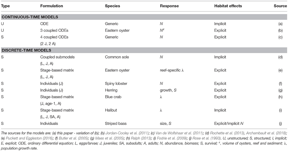
Table 1. Key features of the dynamic models used as examples.

Similar predictions can be obtained from explicit and implicit representations, and both approaches can deal with habitat effects at the population level. Simulating different scenarios of habitat change can be challenging with implicit representations because the new changes in vital rates must be derived external to the model (Diamond et al., 2013). If done appropriately, simulating a habitat change with explicit representation is more straightforward as the habitat variable in the model is simply changed and the resulting effects on vital rates are automatically imposed within the model.

We often mistakenly consider population models to not include effects of habitat unless an explicit representation is present. Models are based on a set of conditions that often include unstated assumptions about habitat conditions and which underlie the values assigned to some parameters. Habitat effects are present in most population models, but are often implicitly part of the formulation and values assigned to parameters, and thus unless parameters related to habitat are subsequently adjusted, the habitat effects are implicitly assumed to remain stable over time.

Incorporation of habitat effects implicitly can be illustrated using the density-dependent, logistic growth model. In this case, the rate of population change is:

$\begin{array}{ll}\frac{dN}{dt}=rN(1-\frac{N}{K})& (1)\end{array}$

where N is population size, t is time, r is the instantaneous rate of population growth per unit time, and K is the carrying capacity of a given habitat in biomass or number of individuals.

The solution to Equation (1) is:

$\begin{array}{ll}{N}_t=\frac{N_{0}K}{N_0+(K-N_0)e^{-rt}}& (2)\end{array}$

where N_t is the population size at time t and N₀ is the initial population size at time t₀.

To model habitat effects implicitly without a specified mechanism, one could presume that an expected loss in habitat will reduce the annual population growth rate by 50% (e.g., from r = 0.4 to 0.2) or lower the carrying capacity by 50% (e.g., from K = 100 to 50). The resulting deviations in the rate of population growth as a function of population size or the population trajectory as a function of time can be solved analytically to determine the quantitative population-level effects of habitat alterations.

Explicit representation of habitat effects requires that the mechanistic relationship (magnitude and shape) between a habitat measure and one or more vital rates (or other model parameters) be specified. The advantages to the explicit approach are that the effects imposed on vital rates in response to changes in habitat are transparent, assumptions are clearly defined, and a mechanistic basis can be identified. However, the data needs shift from long-term monitoring-type data sets based on correlation between habitat and population measures, to data derived from fine-scale, short-term, process-oriented field and laboratory experiments.

A simple example of incorporating habitat explicitly into the logistic growth function applied to oyster comes from Jordan-Cooley et al. (2011). They used the model to understand why high-relief reefs appear to be more stable and sustainable, and specifically how oyster reef height interacts with sediment deposition and possible burial of the oysters to produce alternative stable states. The logistic population growth model was modified as:

$\begin{array}{ll}\frac{dN}{dt}=rN(1-\frac{N}{K})-\mu N-(1-f)\epsilon N,& (3)\end{array}$

where μ is mortality rate from predation and disease year⁻¹, ε is mortality rate due to sediment year⁻¹, and f is a sigmoid function $f=\frac{1}{(1+e^{-\varphi d})}$ with input d used to scale the effect of sediment-induced mortality. The final term in the equation is the explicit habitat effect because mortality rate is a function of a habitat feature, reef height. The variable d reflects habitat quality, which is represented by the difference between population abundance N minus sediment S, and is given by $d=\frac{N}{2}-S$. The function f, which depends on d, is bounded by 0 and 1, and uses the parameter ϕ to adjust the shape of the function. As ϕ increases, the function f has a sharper transition from 0 to 1. In this model, it is assumed that population abundance is unaffected by sediment until more than half of the population is covered by sediment, such as happens on restoration oyster reefs (Colden and Lipcius, 2015).

Specification of Functional Relationships

Habitat-Process Relationships

For both explicit and implicit representations of habitat effects in population models, some quantification of the effects of changes in habitat on organism vital rates is required. The relationships between habitat and vital rates can be independently integrated or interactively linked in the model. An independently integrated relationship is a one-way effect where the habitat only influences vital rates and population dynamics, and is not itself affected. For instance, in the oyster model by Puckett and Eggleston (2016), oyster population dynamics was affected by location and quality of reef habitat, but associated changes in the populations did not affect the features of different habitats. In contrast, the oyster model by Jordan-Cooley et al. (2011) used coupled, mechanistic equations that represented the quality and quantity of reef habitat, which affected oyster population abundance, and oyster abundance in turn affected reef habitat quality and quantity.

Another issue in adding habitat to models is specification of the shape of the relationship between the vital rates and the quantity and quality of habitat. We often have observations or information on vital rates at discrete values of habitat; determining whether there is continuous change in vital rates over the range of habitat values or whether there are threshold effects is difficult. Physical habitat can be simply viewed as having an effect like other environmental variables, such as temperature, whereby vital rates change predictably and continuously over the range of habitat values or as having no effect until habitat goes below a critical level (e.g., threshold response). Distinguishing between these two possibilities is important because they can have very different effects at the population level.

The domain within which the habitat-process relationship is valid and realistic should be defined. We usually have empirical information centered on the baseline condition in simulations. For example, we often use a specific set of experiments to define the habitat-process relationship, and a specific time period to calibrate or validate the population model, which may have its own associated habitat conditions. The habitat-process relationship often has less information at the extremes of habitat characteristics (quality and quantity attributes) and so has higher uncertainty at low and high values of habitat within the specific relationship. When the question involves how new habitat conditions (e.g., loss or restoration) will affect the population, care must be taken to ensure that the new habitat conditions are still within that part of the habitat-process relationship where we have sufficient confidence in its form.

A relationship between habitat and a population's response can be derived that plugs directly into the structure of the population model, or a sub-model external to the population can be developed as part of a hybrid modeling approach. Some adjustment (scaling) is necessary with the hybrid approach because the external sub-models typically apply to a portion of the life cycle under simplified environmental conditions and to a portion of the total spatial area covered by the population model. Two modeling approaches, either separately or combined, that are good candidates for both direct insertion into population models or used as external submodels are Individual Based Models (IBM) and Dynamic Energy Budget (DEB) models (see below).

Density Dependence

Integrating habitat effects into a population model that also includes density dependence in growth, reproduction, mortality, or movement requires careful consideration of the form of the habitat-process relationship. Incorporating density-dependence into population models remains a challenge (Higgins et al., 1997), especially for site-specific applications and models whose results strongly influence management actions (e.g., fisheries stock assessment). Unstructured models appear simpler but specifying how aggregated parameters change in response to abundance or biomass is difficult. Structured and individual-based approaches have easier-to-interpret parameters but often require information on how multiple processes vary by age or life stage in response to abundance or biomass. These issues carry over to situations including habitat considerations in dynamic models.

In many situations, there is representation of density-dependence in an existing population model, and the idea is to add habitat effects to the existing model. Even in the case of a new model being developed in concert with the consideration of habitat, how to include density-dependent effects as part of the habitat or in other life stages entails vigilant formulation. Some of the density-dependent effects may already be due to the habitat effect (double-counting), or adding the habitat effect can distort the overall density-dependent response for which the model was configured or fitted and already deemed realistic. In addition, the form of density dependence requires careful consideration, whether as negative density dependence which has regulatory and stabilizing effects on population dynamics or as positive density dependence which can lead to destabilizing effects, especially under Allee effects at low population abundance.

A common situation when adding habitat effects to a model is when the population model uses a spawner-recruit relationship to encapsulate early life-stage dynamics into a single relationship. Yet, many habitat effects of interest operate on certain life stages, and often multiple life stages differently (e.g., larvae vs. juveniles). The challenge is how to modify the spawner-recruit relationship to allow for changes in different habitats specific to life stages, while maintaining the same original spawner-recruit relationship (Rothschild, 1986). Separating life stages between spawning and recruitment (e.g., eggs, larvae, and young-of-the-year juveniles) makes linking to habitat effects easier but then requires a reformulation of density dependence at the life-stage level to maintain the original spawner-recruit relationship.

Transport and Behavioral Movement

Movement among habitats that differ in quality is a common feature of the life cycle of marine species. The interaction between habitat quality and movement can influence foraging, predator-avoidance, migration, and avoidance of degraded habitats (Watkins and Rose, 2014). Habitat characteristics affect all types of movement because they often serve as the cues determining departure decisions by individuals and selection of destinations, such as larval settlement onto bottom habitat (Stockhausen and Lipcius, 2003; North et al., 2008). The consequences of transport and movement to population dynamics are their effects on the vital rates of growth, mortality, and reproduction rates as the individual experiences different habitat conditions because of its movement to new locations. Simulating larval transport to examine the connectivity of spawning and nursery areas has a long history (Cowen et al., 2000; Levin, 2006). Behavioral modeling of larvae, juveniles and adults using habitat as cues is a relatively recent and rapidly advancing field that combines biophysical modeling, physiology, and movement ecology (Stockhausen and Lipcius, 2003; North et al., 2008; Watkins and Rose, 2013; Allen et al., 2018).

Barbeau and Caswell (1999) provide an excellent example that integrates movement across habitat patches. In their study, a stage-based, multi-patch matrix model was used to quantify the effects of predation and dispersal between patches on sea scallops, Placopecten magellanicus, in nursery habitats. In their system, density-dependent dispersal modulated the effects of predation on scallop abundance.

Habitat Effects within Different Types of Population Models

In this section, we provide details and examples of mathematical and statistical modeling approaches that can be used for quantifying habitat value at the population level (Figure 1). The modeling approaches are first organized as either dynamic (= mathematical) or static (= statistical). We focus on habitat suitability, now subsumed under the newer term of species distribution modeling, which uses statistical methods for fitting and evaluation, within the static model category because they are a very common static model formulation for assessing habitat effects at the population level (Gutiérrez et al., 2005; Vasconcelos et al., 2010). While statistical analyses play an important supporting role (e.g., specification of underlying relationships) in dynamic models, statistical approaches are the major analysis method used in static models. Dynamic models are then presented according to the currency and level of organization followed in the models: unstructured, structured, and individual-based. The features of the dynamic model examples are summarized in Table 1. Our focus is on population models, which includes single-species and multi-species (e.g., predator-prey) models.

FIGURE 1

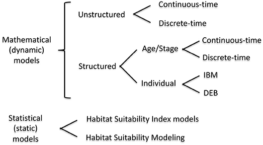
Figure 1. Mathematical modeling approaches that can include habitat variability. IBM, Individual Based Model; DEB, Dynamic Energy Budget model. We do not consider community food web or ecosystem models, such as EcoSpace, in this review.

Unstructured and Structured Population Models

Population models can be considered as unstructured or structured. Unstructured population models assume that all individuals within the modeled population are identical and the state of the population is characterized by one or a few model variables such as total population abundance or biomass. Unstructured models are appropriate for theoretical analyses, populations with simple life cycles, and for analysis of populations with limited information. For many populations, sufficient data are not available to allow division of the population into categories (individual, age, size, or sex), and unstructured population models are then the most suitable option. For other populations, a structured approach is appropriate when vital rates vary among individuals or with age, size, stage, or sex. In this case, model variables characterize categories of the population, which sum up to the total population.

Unstructured models are used less frequently than structured approaches for management decision-making. Notable exceptions are the oyster reef analyses described above that were used to plan and implement oyster reef restoration in Chesapeake Bay (Lipcius et al., 2015), and the application of population models to oyster management (Wilberg et al., 2013) and marine reserves (St. Mary et al., 2000). Fisheries management sometimes uses unstructured models like the logistic formulation for data-limited species (Prager, 2002; Hayes et al., 2009). Increasingly, management questions require more detailed representations of the population to realistically represent changes in vital rates within the life cycle and because management questions are gravitating toward analyses that are better answered with explicit treatment of space. Unstructured approaches do not permit simple treatment of complex life cycles in which life stages use different habitats. However, they do provide insight into general population behavior in the context of habitat-specific questions with relatively little parameterization effort. The simplicity of unstructured approaches is both their strong point and their weakness.

A recent modeling alternative to categorizing a population by age or stage involves defining survival, growth, and reproduction as continuous functions of size and age with Integral Projection Models (IPMs). These models allow for separation of the independent and collective effects of age and size on population dynamics (Ellner and Rees, 2006) and can be parameterized either with empirical data on survival, growth, and reproduction of individuals (Ellner and Rees, 2006) or with empirically derived relationships of survival, growth, and reproduction as a function of size and age (White et al., 2016). Some recent examples of IPMs for marine species include ones dealing with oyster restoration (Moore et al., 2016, 2018), long-distance migration in fish (Färber et al., 2018), and coral and clam population dynamics (Schreiber and Moore, 2018).

An additional classifier we did not consider was whether population models are formulated as deterministic or stochastic. Stochastic formulation implies that values used in simulations of some or all parameters are generated from probability distributions so that the values of those parameters differ through time within a simulation or differ among simulations (Higgins et al., 1997; Mosnier et al., 2015). All of our classes of models can be either deterministic or stochastic; the only difference within a category is whether one needs to know how habitat would affect not only the mean or best estimate of a parameter (deterministic case) but also potentially the variability in those parameter values for thorough adjustment of parameters in stochastic models.

Dynamic Models: Differential Equation (Continuous-Time) Models

Unstructured and structured models are commonly deployed in continuous time (Table 1). Continuous time models, or differential equation models, are suited for time-dependent and equilibrium analysis of the dynamics of the population. In general, this type of model describes a population with one equation, or it consists of multiple equations representing stages or other interacting species. The model may or may not incorporate a spatial component, such as multi-patch models, and habitat effects can be represented implicitly or explicitly. When habitat is explicitly taken into account, this type of model could be used to aid management directly, whereas when habitat is only implicitly integrated into the model more analyses are required to assess management questions related to habitat. For example, an implicit habitat analysis would require external calculations to the model that relate each management action to changes in vital rates or values of specific model parameters. The outcome of this type of model is population dynamics, mostly presented as analytical (e.g., equilibria) or as numerical solutions. Analysis of differential-equation models also permits discovery of conditions for which multiple stable states exist (May, 1976; Scheffer et al., 2012).

As examples of the use of continuous-time models, we describe two modeling efforts (Table 1), one that explicitly models the effects of nursery habitat on the population dynamics of an exploited fish species (Van de Wolfshaar et al., 2011), and another that explicitly examines the effects of habitat upon abundance of an oyster population (Jordan-Cooley et al., 2011).

Van de Wolfshaar et al. (2011) adopted a biomass-based stage-structured model (De Roos et al., 2008) to analyze the consequences of habitat-specific, resource-dependent growth and reproduction for population dynamics. The main advantage of the biomass-based, stage-structured model is its ease of analysis with conventional mathematical techniques used to analyze the behavior of systems of differential equations (Kot, 2001). The model represents a consumer population with a juvenile stage J, an adult stage A, and separate resources for juveniles and adults (R_J and R_A, respectively) corresponding to different juvenile and adult habitats. Hence, juveniles do not compete with adults; intraspecific competition only occurs within each stage. Habitat-specific resources grow at rate δ and equilibrate at carrying capacities R_CJ and R_CA when consumers are absent. Consumption by juveniles and adults follows a Holling Type II functional response (Holling, 1959; Hassell, 1978) with a half-saturation constant H and a mass-specific maximum ingestion rate I_max, which are equal for adults and juveniles. Ingested resources by each stage i are converted with an efficiency minus the metabolic rate, yielding net biomass production υ_i(R_i) of each stage when feeding on a particular resource R_i. A set of four differential equations describes the biomass dynamics of the resources, juveniles and adults:

$\begin{array}{ll}\frac{d{R}_A}{dt}=\delta (R_{CA}-R_A)-\frac{R_A}{H+R_A}{I}_{max}A& (4)\end{array}$

$\begin{array}{ll}\frac{d{R}_J}{dt}=\delta (R_{CJ}-R_J)-\frac{R_J}{H+R_J}{I}_{max}J& (5)\end{array}$

$\begin{array}{ll}\frac{dJ}{dt}={\upsilon }_A^{+}{R}_{A}A+{\upsilon }_J{R}_{J}J-\gamma {\upsilon }_J^{+}{R}_{J}J-{\mu }_{J}J& (6)\end{array}$

$\begin{array}{ll}\frac{dA}{dt}={\upsilon }_A{R}_{A}A-{\upsilon }_A^{+}{R}_{A}A+\gamma {\upsilon }_J^{+}{R}_{J}J-{\mu }_{A}A& (7)\end{array}$

where μ_i is the mortality rate in stage i, $\gamma {\upsilon }_J^{+}{R}_J$ is the rate at which juveniles mature into the adult stage, and ${\upsilon }_A^{+}{R}_A$ is the reproduction rate. The maturation rate of juveniles depends on the net biomass production of the juvenile stage, the size range over which juveniles grow from egg to adult, and juvenile mortality. All surplus adult biomass is converted into offspring, such that reproductive rate equals net biomass production of adults. Biomass can only be transferred between stages when net biomass is produced. Conversely, when net biomass production is negative, the stage suffers starvation mortality, and neither recruitment nor maturation occurs.

In the Van de Wolfshaar et al. (2011) model habitats were defined as exclusive adult and juvenile habitats with separate resources (i.e., prey). The modeled habitats were generalized and not specific to any particular fish species. Habitat was integrated explicitly into the model because reproductive rate depended explicitly on the amount of resource (prey) in juvenile and adult habitats; mortality rates were not dependent on habitat.

Van de Wolfshaar et al. (2011) explored the consequences of differing productivity in juvenile and adult habitats by adopting a baseline resource carrying capacity in both habitats R_max that was scaled as $R_{CJ}=e^x{R}_{max}$ and $R_{CA}=\frac{1}{e^x}{R}_{max}$. At x = 0, juvenile and adult habitats are equally productive, whereas when x < 0, adult habitat is more productive than the juvenile habitat and vice versa. Hence, habitat is modeled directly by modifying the relative productivity of juvenile and adult habitats, which are assumed to be equal in area. The relative difference in habitat productivity as a function of scalar x is shown in Figure 2. Differences in relative productivity between juvenile and adult habitats produced alternative stable states with more biomass in either the juvenile or the adult stage. When fishing mortality was added to the model, the simulations showed that improving juvenile habitat was more effective in increasing adult biomass than a reduction in fishing mortality of adults. A similar stage-structured approach was applied to model the effects of offshore migration of juvenile plaice (Pleuronectes platessa) into adult habitat, and its consequences on population dynamics and fisheries yield (Van de Wolfshaar et al., 2015).

FIGURE 2

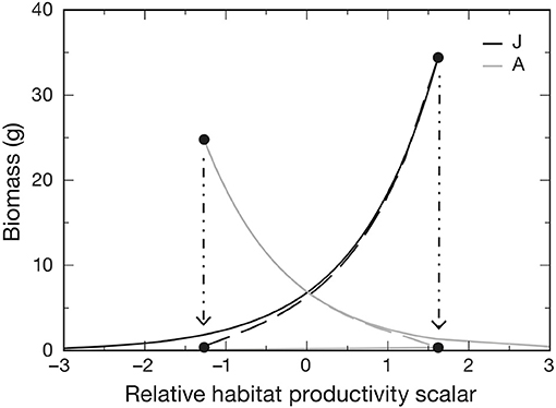
Figure 2. Biomass of adult A and juvenile J life stages as a function of relative habitat productivity (x) showing where stages are under stable (solid lines) and unstable (dashed lines) equilibria. Alternative stable states occur between the hatched arrows, at which one of the alternative equilibria collapses and beyond which only one stable equilibrium occurs. Adult μ_A and juvenile μ_J mortality rates were both set to 0.05. Figure reproduced with permission (Inter-Research) from Van de Wolfshaar et al. (2011).

Jordan-Cooley et al. (2011) used a set of differential equations in an unstructured model that explicitly integrated habitat (i.e., reef height effect on mortality) to study the effects of live oysters, dead oysters (reef matrix), and sediment deposition rates on the viability of oyster reefs. The model analyzed the rate of change in volume per m² of live oysters N, dead oyster shell R, and deposited sediment S on an oyster reef with respect to time t in years. The collective volume of live oysters, dead oyster shell, and deposited sediment therefore represents an oyster reef. The volume per m² can be converted directly to reef height because it is calculated as the volume of a 1-m² unit area.

In the Jordan-Cooley et al. (2011) model habitats (i.e., oyster reefs) were defined by the volumes of live oysters, dead oyster shell, and sediment on the reef. Habitat was integrated explicitly into the model because reproduction and survival were dependent on functions of live oyster volume, dead oyster shell volume, and sediment volume on the reef.

Live oyster volume N(t) in m³ (equivalent to reef height in m for a 1-m² area) is represented by Equation 3, with $d=\frac{N}{2}+R-S$ and therefore dynamic in a complicated way because all three variables vary with time and depend on the state of the system. We used the same example (Jordan-Cooley et al., 2011) earlier to illustrate explicit treatment of habitat in a logistic model. Continuing with Equation 3, terms for natural mortality due to disease and predation (μ) and mortality due to burial by sediment ε were added separately to the logistic formulation that already included mortality as part of r; the estimate for r was therefore increased accordingly to avoid double-counting of mortality sources. An important feature of f in Equations (3, 8, and 9) is that its effect within the unstructured logistic equation is an aggregate effect on the change in biomass and therefore is non-specific as to how habitat affects reproduction, growth, and recruitment.

The rate of change in dead oyster shell volume R is modeled as:

$\begin{array}{ll}\frac{dR}{dt}=f\mu N+(1-f)\epsilon N-\gamma R,& (8)\end{array}$

where the two positive terms come from the death of live oysters in Equation (3) and γ is the rate of loss of dead oyster shell due to degradation year⁻¹.

The rate of change in sediment volume on the oyster reef is:

$\begin{array}{ll}\frac{dS}{dt}=-\beta S+Cg{e}^{-\frac{FN}{Cg}}.& (9)\end{array}$

where the first term is the rate of sediment erosion with a rate β; the volume of eroded sediment is proportional to the volume of deposited sediment. The second term is the rate of sediment deposition, which in the absence of oysters is C·g, where C is a maximum possible deposition rate and g is a decreasing function of reef height (N + R). The deposition rate is maximal at the seafloor, and decreases as the reef height in the water column increases. Biodeposition is a constant fraction of sediment deposition. Filtration rate F per unit oyster volume depends on the height-dependent sediment concentration, which is proportional to C·g:

$\begin{array}{ll}F=\frac{F_{max}}{{\left[Cg\right]}_{max}}\left[Cg\right]e^{\frac{{\left[Cg\right]}_{max}-\left[Cg\right]}{{\left[Cg\right]}_{max}}},& (10)\end{array}$

where F_max is the maximum filtration rate, which occurs at [Cg]_max. The rate F scales linearly with C when C is low, it reaches a peak at some intermediate, optimal sediment concentration, and beyond this it decreases as oyster gills become clogged. The sediment concentration [Cg] is that impinging on the reef at the reef surface. The filtration function assumes that sediments filtered by oysters are either expelled and move off the reef, or they become part of the underlying reef matrix and no longer cover living oysters.

The model using equations for N (Equation 3), R (Equation 8), and S (Equation 9) examined the possibility and conditions for alternative stable states in oyster reefs (Figure 3). Analysis of the system of equations indicated that alternative stable states were possible, and that the initial height of the oyster reef determines the equilibrium state through its effects on mortality rates (Jordan-Cooley et al., 2011). Only when the initial reef height exceeded a threshold did the oyster reef persist at a positive equilibrium (i.e., left panel of Figure 3); below the threshold the oyster reef degraded to extinction as oysters were unable to compensate for increased sediment deposition (i.e., right panel of Figure 3).

FIGURE 3

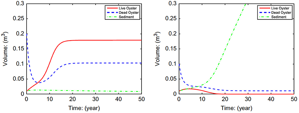
Figure 3. Simulations of volume of live eastern oysters N (Crassostrea virginica), dead oyster reef R, and sediment S as a function of initial reef height R_{t = 0}, demonstrating alternative stable states of a positive equilibrium (left) and extinction (right). For all cases N_{t = 0} = 0.01 and S_{t = 0} = 0.01. (upper left) R_{t = 0} = 0.20; (upper right) R_{t = 0} = 0.10. Figure reproduced with permission (Elsevier license 4451990372334) from Jordan-Cooley et al. (2011).

Dynamic Models: Matrix and Difference Equation (Discrete-Time) Models

Most discrete-time models in population dynamics are based on a structured approach (Table 1). Given the complex life histories of most marine species, which include larval, juvenile, and adult phases that use different habitats, populations can be expressed as a series of connected age, size, or stage classes (Table 1). The basic form of these life histories is depicted in a life-cycle diagram (Figure 4) and converted to a system of linked difference equations, and in many cases, into a matrix projection formulation that predicts the population vector at time t+1 from the vector at time t (Figure 5). The matrix formulation is a special case of the more general structured, discrete-time models in which elements of the matrix are the transition probabilities and the top row is fecundity (Leslie, 1945; Lefkovitch, 1965; Caswell, 2001). We first present a structured (but not matrix) discrete-time model that implicitly examines habitat effects on the juveniles of common sole Solea solea (Rochette et al., 2013). We then use three examples that use matrix formulations. The models of blue crab Callinectes sapidus by Ralph (2013) and eastern oyster Crassostrea virginica by Theuerkauf (2017) illustrate how habitat effects can be analyzed explicitly, whereas the Fodrie et al. (2009) model of California halibut Paralichthys californicus illustrates how matrix-based population models can be used with an implicit treatment of habitat effects.

FIGURE 4

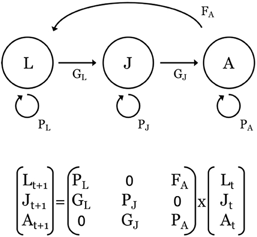
Figure 4. Top: Representative stage-based, life-cycle diagram and associated transitions (F, G, P) of a population defined by three stages: larvae (L); juveniles (J), and adults (A). F = fecundity, defined as the number of offspring, P = probability of survival and remaining within a stage, and G = probability of survival and growing into the next stage. Bottom: Corresponding projection matrix and population vectors at times t and t+1 for the population described above. The time step is usually one year. For species that make ontogenetic migrations across larval, juvenile, and adult life-history stages, the G parameters are often associated with a switch in habitat use.

FIGURE 5

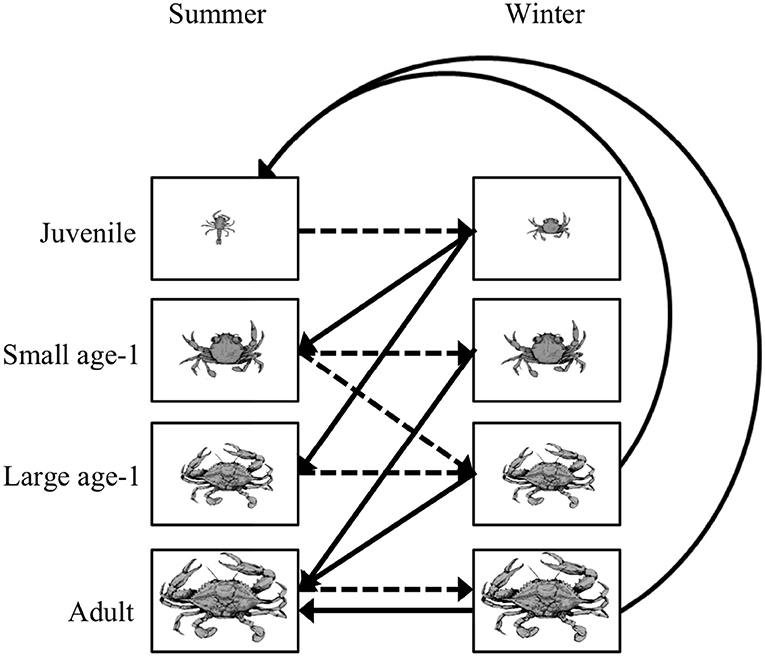
Figure 5. Life cycle diagram for the blue crab Callinectes sapidus. An individual crab can be in one of four stages: juvenile, small age-1, large age-1, and adult during the summer and winter. Summer to winter transitions are represented by the dashed lines, while the winter to summer transitions are represented by the solid lines. All transitions have a 6-month time step. Note that survival and growth probabilities are straight lines, while the fecundity terms are curved lines. Figure reproduced with permission (G. Ralph, copyright holder) from Ralph (2013).

Rochette et al. (2013) and then Archambault et al. (2018) developed a Bayesian state-space, full life-cycle model for common sole in the eastern English Channel. The model includes different modules representing key processes acting in specific, spatially separated habitats: (1) a population model for adults, (2) a Lagrangian drift model for eggs and larvae settling to different near-shore estuaries, and (3) a juvenile habitat suitability module. This type of model allows various interacting pressures to be examined and compared for their effects on the population, such as fishing pressure on adults, climate-driven variability in drift routes of larvae, and habitat suitability of juvenile nursery habitats. Habitats were defined as five different nursey habitat sectors. Habitat was integrated implicitly into the model because mortality rates in nursery habitats were estimated by the relative abundance of age 0 and age 1 juveniles.

A habitat suitability model, based on juvenile trawl surveys coupled with a geographic information system, was used to estimate juvenile densities and areas of suitable juvenile habitat in each nursery sector. Rochette et al. (2013) estimated the value of habitat of the five nursery areas, and demonstrated that the value was not proportional to the area of each habitat (Figure 6). Archambault et al. (2018) used the model to show the importance of nursery habitat area and quality for common sole. Simulating nursery habitat recovery (both surface area and quality) in one single estuary, the Bay of Seine, demonstrated that the population would increase by two-thirds and the effects would carry over to the adjacent subpopulation and affect fishery yield.

FIGURE 6

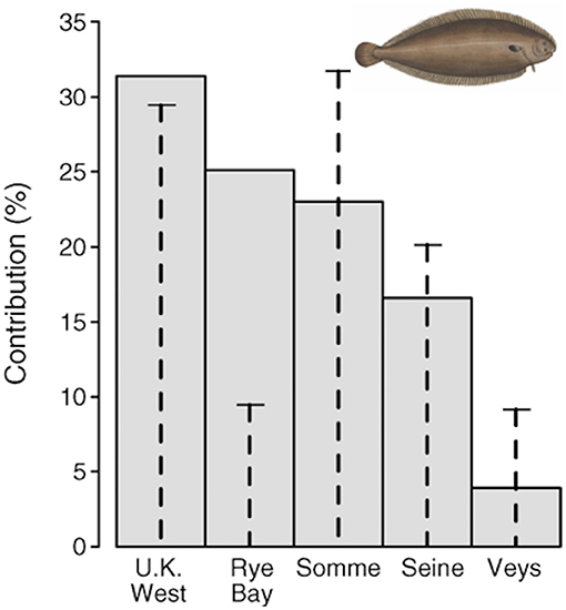
Figure 6. Contribution of each nursery ground to the total recruitment of age-0 juveniles of common sole Solea solea in the Eastern Channel. Gray bars are the average contribution (calculated across all years) of each nursery to total recruitment. Vertical dashed lines indicate the surface area of each nursery as a percentage of the total surface area of nursery sectors, so that the difference between bars and dashed lines highlights the contrast in productivity. Figure reproduced with permission (Wiley and Sons license 4454871465571) from Rochette et al. (2013). Image from https://www.wpclipart.com/animals/aquatic/fish/F/flatfish/Common_sole__Solea_solea_2.png.html.

Projecting changes in population size (and age or stage structure) using matrix formulations can be simulated by matrix multiplication over a selected time period, while the long-term (asymptotic) behavior is defined analytically by the dominant eigenvalue (i.e., λ) of the projection matrix for density-independent rates (Caswell, 2001). Note, however, that matrix multiplication when the starting age distribution is not close to the stable age distribution may produce transient, not asymptotic, dynamics (Hastings et al., 2018). To avoid the problem of transient dynamics in matrix multiplication, it is best to use eigenanalysis for deterministic models. For stochastic models, population projection is needed and the stochastic λ will be less than the asymptotic λ for the same model as a deterministic model. In the density-independent case, λ integrates vital rates from all life-history stages into a single measure of overall population fitness, and therefore provides a clear and easily understandable metric of habitat value. Density-dependent matrices require more complex analyses and yield metrics of habitat value under stricter assumptions than density-independent matrices (Caswell and Takada, 2004).

Implicit and explicit integration of habitat can be accomplished by analyzing a population projection matrix developed for a life-cycle diagram (e.g., Figures 4, 5), then re-analyzing the model after altering one or more transition probabilities (F, G, P) that reflect habitat effects, and examining the change in λ. For example, Ralph (2013) investigated the effect of varying seagrass nursery area for blue crab juveniles on λ (Figure 5). The life-cycle diagram is more complex than the one in Figure 4 because Ralph (2013) developed separate spatially-explicit projection matrices on a semi-annual time step for summer and winter seasons (Figure 5). Habitats were defined as vegetated and unvegetated juvenile nurseries. Vegetated habitats were generally seagrass beds, whereas unvegetated habitats were mud and sand subtidal flats. Habitat was integrated explicitly because mortality rates of juveniles in vegetated and unvegetated nurseries were varied based on field experiments of juvenile survival. The analysis demonstrated that λ could be increased from negative to positive population growth by increasing the area of seagrass nursery habitat.

Implicit integration of habitat in a matrix model that also uses the finite population growth rate comes from Fodrie et al. (2009). They considered the demographic consequences related to utilization of nursery habitat alternatives by juvenile California halibut. Habitats were defined as four juvenile nursery habitats (exposed coast, bay, lagoon, and estuary). Bays were characterized by low-tide surface areas >84 ha, average depths >4 m, and area-to-perimeter ratios >10 ha km⁻¹. Lagoons were characterized by low-tide surface areas of 35 to 84 ha km⁻¹, average depths of 3 m, and area-to-perimeter ratios between 2.4 and 8.4 ha km⁻¹. Estuaries were described by low-tide surface areas <25 ha and average depths <2.5 m. Estuaries were also characterized by high wetland (salt marsh) cover, resulting in low area-to-perimeter ratios (<2 ha km⁻¹). Exposed coast consisted of shallow-water, exposed coastal habitat. Habitat was integrated implicitly by using habitat-specific densities in cohort life tables to estimate mortality rates.

Recently, the most widely-used metrics of nursery value have been total production of individuals to an adult stock or unit-area production to an adult stock (Sheaves et al., 2015). Fodrie et al. (2009) demonstrated that these metrics of nursery “value” can be decoupled from the impacts of nursery use on λ. Although alternative juvenile habitats (exposed coast and coastal embayments) could contribute an approximately equal number of recruits to the adult stock, positive population growth (λ > 1) depended critically on the subpopulations of juveniles that utilized coastal embayments, such as bays, lagoons, and estuaries (Figures 4, 7). Conversely, the juvenile subpopulation along the exposed coast contributed negatively to overall population growth (λ < 1) in three of the 4 years of the study due to elevated juvenile mortality in that habitat (Figure 7).

FIGURE 7

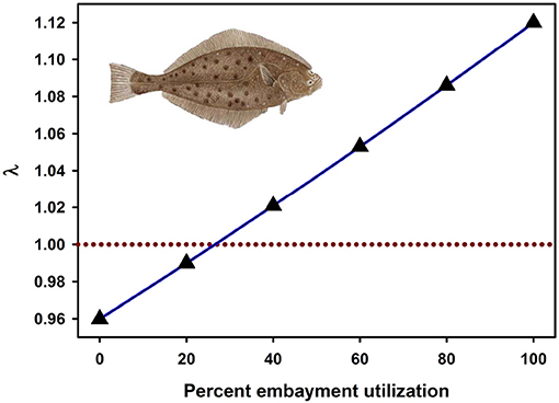
Figure 7. Fitness of a California halibut Paralichthys californicus population resulting from the percentage of juvenile fish that utilized exposed coast vs. embayment habitat as nurseries during 1987, 1988, 2002, and 2003. Dashed line represents a stable population (λ = 1). Figure adapted with permission (Inter-Research) from Fodrie et al. (2009). Image from http://www.channelislandssportfishing.com/halibut-fishing-california.

Effective management requires incorporation of spatial ecology and subpopulation connectivity into management plans, and matrix projection models are amenable to metapopulation modeling approaches in which multiple subpopulations are connected via dispersal, emigration, and immigration of larvae. Moreover, comprehensive evaluation of how habitats affect metapopulation source-sink dynamics (Lipcius and Ralph, 2011) is needed to inform application of metapopulation concepts in spatial management of populations connected via larval dispersal (Botsford et al., 2003; Figueira and Crowder, 2006; Lipcius et al., 2008, 2015; Holstein et al., 2015; Puckett and Eggleston, 2016). Recently, Theuerkauf (2017) adapted a size-structured, discrete-time matrix metapopulation model (Puckett and Eggleston, 2016) to explore local and regional population dynamics of exploited bivalves; in this case 646 reefs of the eastern oyster in Pamlico and Core Sounds, North Carolina served as habitat. The metapopulation model: (1) evaluated the spatial distribution, areal footprint, and initial population size of all oyster reef types within the estuary, (2) determined transition probabilities by reef type and intra-annual oyster size classes explicitly with field data, (3) determined size-specific oyster fecundity estimates, (4) quantified local larval retention and inter-reef connectivity via larval dispersal simulations, (5) simulated metapopulation dynamics throughout the estuary using a demographic matrix model over 5 years (2012-2016), and (6) evaluated consistency in metapopulation source-sink structure over space and time. Each reef's contribution to the metapopulation was calculated based on whether the reef-specific (local) population growth rate (λ_c) was positive or negative (Figueira and Crowder, 2006). For the May-June spawning and recruitment periods, subtidal no-take sanctuaries were the only reef type with a mean λ_c>1 and thus acting as sources (Figure 8); reefs serving frequently as sources were generally located in the northeastern portion of Pamlico Sound (Figure 9). Importantly, the results of the modeling were validated with extensive field data (Figure 10), which should be attempted whenever modeling exploited populations.

FIGURE 8

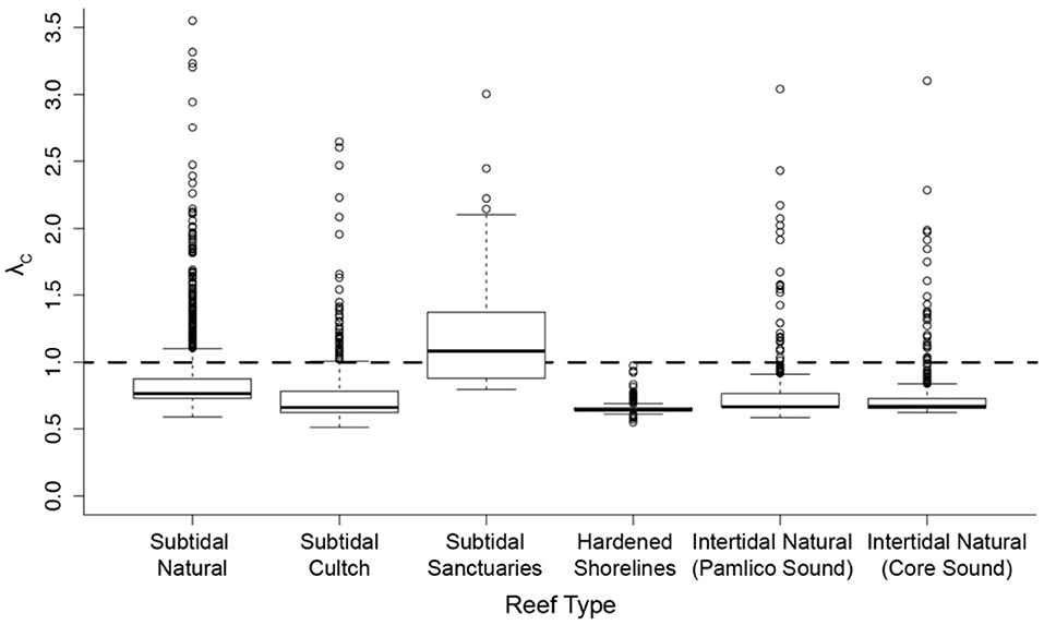
Figure 8. Spatiotemporal variation in metapopulation oyster reef source vs. sink status according to oyster reef type for the eastern oyster Crassostrea virginica. Subtidal cultch (= settlement substrate) reefs are those in which the North Carolina Division of Marine Fisheries (NCDMF) spreads oyster shells or other substrate on the estuarine bottom, followed by natural oyster larval settlement and growth, and harvest by the fishery when oysters reach legal size. Subtidal sanctuaries are oyster reefs generally created by the NCDMF, and are no-harvest, broodstock reefs. Hardened shorelines include pilings, sea-walls and rock rip-rap. Intertidal reefs include those natural intertidal oyster reefs located in two water bodies, each with varying mean demographic rates. Source-sink status (λ_c) of each reef (by reef type) during each May-June time step between 2012-2016 (assuming larval mortality rate of 10% day⁻¹). λ_c ≥ 1 indicates that a given reef functioned as a source during time t, and λ_c < 1 as a sink. Figure adapted with permission (S. Theuerkauf, copyright holder) from Theuerkauf (2017).

FIGURE 9

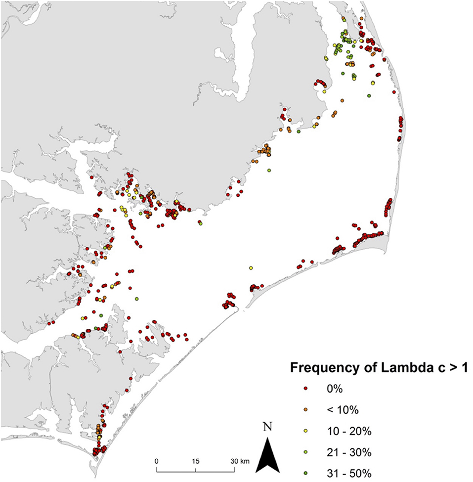
Figure 9. Spatiotemporal variation in metapopulation source vs. sink status for eastern oyster Crassostrea virginica. Frequency of λ_c ≥ 1 at all reefs across the five-year model time frame (assuming a larval mortality rate of 10% day⁻¹). λ_c ≥ 1 indicates that a reef functioned as a source during time t, and λ_c < 1 as a sink. Green dots represent frequent ‘source’ reefs (i.e., λ_c ≥ 1, 31-50% of the time), red dots represent ‘sink’ reefs (i.e, λ_c ≥ 1, 0% of the time). Figure adapted with permission (S. Theuerkauf, copyright holder) from Theuerkauf (2017).

FIGURE 10

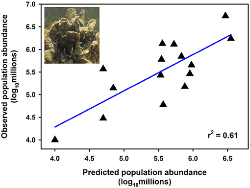
Figure 10. Relationship between observed and predicted population size of oysters using a metapopulation model at natural subtidal and restored reefs of eastern oyster Crassostrea virginica. Estimates of observed population size were derived from field sampling of natural subtidal and restored reefs during 2012; estimates of predicted population size were derived from metapopulation model simulations corresponding to the same time period (assuming a larval mortality rate of 10% day⁻¹). Linear least-squares regression of log₁₀-transformed data (p < 0.001). Figure adapted with permission (S. Theuerkauf, copyright holder) from Theuerkauf (2017). Oyster figure derived from http://cbf.typepad.com/chesapeake_bay_foundation/2015/04/restoring-the-coral-reefs-of-the-chesapeake.html.

Dynamic Models: Individual-Based Models

Individual-based models (IBMs) operate by tracking the traits of individuals as they are affected by growth, movement, reproduction, and mortality (DeAngelis and Mooij, 2005). The higher-order outcomes, such as population abundance, average weight-by-age, and spatial distributions, are the sum (or average) of the traits of the individuals in time and space (Grimm and Railsback, 2013). IBMs can be considered a more resolved, structured approach than the widely-used matrix (age- and stage-based) projection model (Caswell, 2001), which follows groups of individuals as a state variable (e.g., number of individuals in an age-class). Like IBMs, the physiologically-structured population modeling approach (De Roos et al., 1992; Metz and De Roos, 1992) also explicitly shows inter-individual variability and, like IBMs, can be used to implicitly and explicitly assess habitat effects on population dynamics (Table 1). Our discussion focuses on IBMs but applies to individual-based approaches in general.

IBMs simulate discrete individuals and thus allow for the time history of what each individual experiences (e.g., temperature, food) to be recorded. The flexibility of IBMs allows for many choices of the traits of individuals to be followed, and the rules and processes on how these traits change with an organism's internal state and environmental conditions, and thus the structure of many IBMs, are highly influenced by the modeler's decisions. Also, data to calibrate and validate an IBM are needed at both the individual level and the population and higher levels (Railsback et al., 2002); both are rarely available for most systems. Unlike matrix projection and physiologically-structured approaches, IBMs are not grounded in a rigorous mathematical framework and therefore their analyses, interpretation, and documentation vary greatly, making evaluation and comparisons difficult (Grimm et al., 2006; Grimm and Railsback, 2013; DeAngelis and Grimm, 2014).

Habitat considerations are included in many IBMs of coastal fish and shellfish (Rose, 2000; DeAngelis and Mooij, 2005; DeAngelis and Grimm, 2014). Often, habitat is included with habitat conditions underlying the specification of process parameter values and calibration and validation data that are used in model development and testing. Each IBM has a domain of applicability that is defined by the conditions (including habitat) for which one remains confident in model realism (Rose et al., 2015b). As one moves outside this domain and into new parameter values and population and habitat conditions, the confidence in model predictions diminishes due to increasing uncertainty whether the model structure and testing (validation) results still apply under the new conditions. Thus, adding to the difficulty in documenting IBMs is the need to document and test both implicit and explicit representations of habitat effects within the models.

IBMs can be useful as a submodel for specific life stages and habitats because the effects of habitat can be inserted into the model to represent habitat effects on individuals measured in the field or laboratory. The IBM then scales these effects on individuals up to higher levels, such as recruitment or numbers surviving to a certain stage. The challenge with IBMs is that they are often applied on fine spatial and temporal scales for a selected area, and the predictions are representative of that area or area type but difficult to generalize to a population or community level. IBMs can be used to simulate specific key life stages, such as egg to recruitment survival (Rose and Cowan, 1993) and migratory route effects on juvenile survival and growth (Maes et al., 2005). In full life-cycle models, including spatially explicit, the young for the next year come from the adults within the model (Rose et al., 2015a), which permits examination of multi-generation effects of habitat but also requires information on all life stages.

We use three IBM analyses to illustrate how IBMs can be used to address fundamental and frequently encountered questions related to habitat and coastal fish and shellfish (Rose et al., 1993; Butler et al., 2005; Maes et al., 2005). The analysis of Rose et al. (1993) illustrates a mix of implicit and explicit analysis of habitat effects on striped bass Morone saxatilis recruitment, while Butler et al. (2005) illustrates an explicit analysis of how changes in habitat affect spiny lobster Panulirus argus recruitment in the Florida Keys (Table 1). The example by Maes et al. (2005), like Butler et al. (2005), also illustrates an explicit analysis but using a dynamic, state-variable approach to identify optimal habitat use of juvenile North Sea herring Clupea harengus (Table 1).

Rose et al. (1993) used an IBM of striped bass (Rose and Cowan, 1993) to examine habitat effects on recruitment with a mix of implicit and explicit integration of habitat effects. The habitat consisted of a single patch (volume = 7.84 million m³) for 100 spawning females and resultant eggs, larvae, and juveniles. Temperature, toxins, and bottom area were varied with functions relating these variables to growth, prey availability, and mortality of eggs, larvae, and juveniles. Larval mortality was explicitly integrated into the model as a function of temperature derived from lab experiments (Morgan et al., 1981). In contrast, juvenile mortality was incorporated implicitly; bottom area of the patch was reduced from baseline to mimic crowded conditions and fewer benthic prey for juveniles due to warm temperature-low DO squeeze.

The model started with a specified set of female spawners, and their eggs were then followed daily as they became yolk-sac larvae, larvae, and juveniles until reaching age-1. Environmental variables were daily temperature and daily densities of zooplankton and benthic prey. Eggs and yolk-sac larvae developed based on temperature; larvae and juveniles grew in weight using a bioenergetics equation with a feeding submodel that combined preferences with densities of the different prey types in a type-II functional response of predators to prey (Holling, 1959; Hassell, 1978). Mortality rate was assumed constant for eggs and yolk-sac larvae, and decreased with size (length determined from weight) for larvae and juveniles. All simulations started with the same number and size of female spawners and the basic comparisons were based on the predicted recruitment (number of individuals surviving to age-1).

A suite of habitat effects was examined by varying model inputs (e.g., warmer temperatures), imposing changes to model parameter values related to mortality rate (either total mortality or based on degree of feeding activity), growth rate, and capture success of prey, or by changing the shape of the model spatial box to force crowded conditions, which reflects intraspecific competition. Both chronic changes, which affected all individuals in a life stage for the entire time, or episodic changes (e.g., mimicking a few days of warmer temperature or a toxic spill event) were simulated. While the temperature effects were explicit, as temperature was a direct input into the model, other effects such as increased mortality, reduced feeding success, and reduced juvenile physical habitat were realistic but imposed implicitly by forcing these changes. Chronic changes to mortality imposed on eggs and larvae generally resulted in the largest reductions in recruitment, whereas reduction in bottom area of juveniles (50% and even 90%) had smaller effects. The analysis illustrates how explicit and implicit analyses can be combined, enabling comparison of chronic and episodic effects across habitat-related stressors such as temperature, toxics, and reduced physical habitat.

Butler et al. (2005) simulated spiny lobster survival in Florida Bay from 1988 to 1996 starting at settlement through emigration to adult habitat about 18 months later. Daily growth (molting), survival, and movement of individuals was simulated in a 7 × 35 grid of cells configured for the strip of Florida Bay bordering the Florida Keys. Each cell was characterized by specified percentages of different habitats (sponges, solution holes, other shelters, and open space). Starting with incoming post-larval lobster, daily growth was based on temperature and mortality was dependent on habitat type. Each day lobsters left their shelters to forage and then competed for preferred shelters (scramble) upon their return. A suite of size-based rules was used to simulate site selection of the daily returning lobsters. Habitat losses due to algal blooms were simulated by reducing abundances (e.g., 60% reduction in 20% of grid cells for 7 months) of loggerhead and other sponges (i.e., preferred habitats) in selected grid cells.

Habitat was a multi-patch grid of 245 cells of nursery habitat. Nursery habitats were characterized as open bottom, seagrass, and hard-bottom habitats. Hard-bottom cells were further described as loggerhead sponge, other sponges, solution holes, octocoral-sponge complexes, and other shelters, mainly scleractinian corals. Habitat was incorporated explicitly because mortality and movement in each habitat were measured empirically through field experiments and mark-recapture studies, respectively. Habitat-specific carrying capacities, which influenced movement rates, were estimated from field densities. Surprisingly, predicted population abundances without and with the algal blooms were similar, even though the loss of habitat caused dramatic shifts in the shelter types used by the lobsters.

Maes et al. (2005) examined how different migration paths of individual juvenile herring in the North Sea would affect growth and survival over a 2-year simulation. Five nursery habitats were defined, ranging from the upper estuary to open sea, which differed in temperature, turbidity, and copepod density. Temperature affected growth and mortality via predation risk; turbidity and copepod density affected feeding tactics; and turbidity also affected predation risk. Habitats were nurseries where whiting preyed on herring. In the estuaries temperature and turbidity varied systematically across environmental gradients, and affected predation intensity by whiting on herring. Habitat was built into the model explicitly because the survival of herring was dependent on consumption rates of whiting, which were specific functions of temperature and turbidity.

The approach used a forward iteration approach with 1-week time steps to determine the optimal (maximum growth and survival) usage of the five habitats over the 2-year period (Figure 11). Weekly usage of the habitat (and resulting weight) were then compared for alternative assumptions such as no predation risk, and spatially-constant temperature, turbidity, or copepod density. The advantages of optimal migration routes were assessed by comparing predicted final body weight and survival under the optimal route with that predicted under random movements and no migration. They concluded that estuarine residence resulted in fitter individuals because of higher survival at the expense of slowed growth.

FIGURE 11

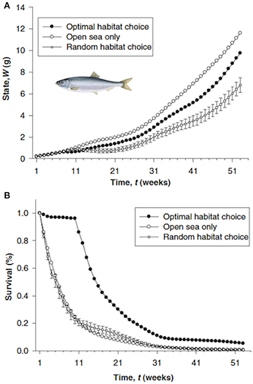
Figure 11. States over time (A) and cumulative survival (B) of three different migration strategies for North Sea herring Clupea harengus (Maes et al., 2005): optimal habitat choice, a forced stay at open sea, and random habitat choice. Errors bars for the random migration represent standard errors of the means of 10 randomized trajectories drawn from a uniform distribution. Time (in weeks) begins on 15 April 1989 (week 1) and ends on 30 March 1990 (week 52). Figure reproduced with permission (Wiley and Sons license 4452010896683) from Maes et al. (2005). Herring figure derived from https://fisheries.msc.org/en/fisheries/spsg-ltd-north-sea-herring/about/.

The preceding IBMs are stand-alone models. Radchuk et al. (2016) made pairwise comparisons between population-based and individual-based models for a range of organisms, including a few marine taxa. They contrasted the performance of the two model types when used as Population Viability Analysis (PVA) models to estimate extinction risk under different scenarios. Their main findings were that the availability and resolution of demographic, spatial, and dispersal data were the primary determinants of the choice of model complexity, while the specific model purpose appeared to be unimportant when deciding on a population- or individual-based model.

Role of Dynamic Energy Budget Models

Martin et al. (2012) made a plea for using Dynamic Energy Budget (DEB) theory (Van der Meer, 2006; Kooijman, 2010; Nisbet et al., 2010) as a unifying framework to describe the role of individual organisms in terms of the acquisition of resources, the allocation to maintenance, growth and reproduction, and the consequences for survival. DEB theory also highlights the central role of the individual in studies of mass and energy balances, and as such is an ideal basis for IBMs and other individual-based approaches. The standard DEB model can in principle be used for all animal species; only the parameters will differ among species. As Martin et al. (2012) write, “DEB is appropriate as a building block for IBMs because it is a relatively simple model that translates environmental conditions to individual performance (growth, survival and reproduction) and is consistent with first principles such as conservation of energy. This is important because the tradeoffs in life-history traits that DEB specifies (e.g., growth vs. reproduction, time and size to maturation) strongly influence population dynamics. Moreover, because DEB is a generic theory, it can be applied to virtually all species, which would facilitate broader insight from specific studies and comparisons between species.” DEB models have been used to model the population dynamics of marine species (Kooi and Van der Meer, 2010; van der Meer et al., 2011), but not with a strong emphasis on the effects of spatial variation in environmental and habitat conditions. Use of the DEB approach, with its well-established formulation and application protocols, will help with the synthesis and integration of IBMs across species and habitat analyses.

Static Models

Statistical modeling techniques are proficient in accommodating the relationship between fish species distribution and surrounding environmental features (Guisan et al., 2002). Various statistical methods have been used to quantify this relationship for several life stages of numerous species, namely: (1) to identify environmental variables that define species distributions, (2) to fit species spatial distribution and predict distribution for a given set of environmental variables, and (3) to map realized and potential habitat for a species.

Two commonly used statistical approaches are habitat suitability index (HSI) models and habitat suitability modeling (U.S. Fish and Wildlife Service, 1980). HSI models consist of a spatial approach that scores habitat suitability based on previous knowledge on habitat use by the species (Brown and Hartwick, 1988; Pollack et al., 2012; Theuerkauf and Lipcius, 2016). First, a spatially resolved habitat map is built for each environmental feature and the habitat map is reclassified to a 0-1 suitability index scale in each grid cell, where 1 is optimal and 0 is unsuitable, based on habitat associations or requirements of the species described in literature. Then, the geometric mean of the suitability index values for all habitat variables is calculated by grid cell, and the results mapped. HSI models have been commonly used in efforts to conserve and restore populations and biodiversity.

For example, Theuerkauf and Lipcius (2016) developed and validated a habitat suitability index model to characterize optimal restoration habitats for eastern oyster in Chesapeake Bay. The HSI was based on substrate type, water depth, and salinity (Figure 12), which affect oyster demographic rates and reef persistence. The obtained HSI mapping was compared with a mapping of oyster density derived from independent field surveys (Figure 13), which validated the HSI model and demonstrated that the HSI is a reliable predictor of oyster abundance and reef persistence.

FIGURE 12

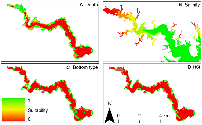
Figure 12. Habitat Suitability Index model for eastern oyster Crassostrea virginica. (A) Depth suitability layer. (B) Salinity suitability layer. (C) Bottom type suitability layer. (D) Habitat suitability index output: red areas are unsuitable oyster habitat, green areas are optimal oyster habitat in the Great Wicomico River, a western shore tributary of lower Chesapeake Bay. Figure reproduced with permission (Creative Commons Attribution 4.0 International Public License) from Theuerkauf and Lipcius (2016).

FIGURE 13

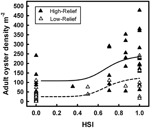
Figure 13. Sigmoidal relationships between habitat suitability index score and associated live adult oyster density on high-relief and low-relief reefs of eastern oyster Crassostrea virginica in the Great Wicomico River, a western shore tributary of lower Chesapeake Bay. Figure reproduced with permission (Creative Commons Attribution 4.0 International Public License) from Theuerkauf and Lipcius (2016).

Habitat suitability modeling approaches rely more on statistical analyses than HSI models, and are based on the fitting of a statistical model to quantify the relationship between species abundance distribution and environmental variables. Ultimately, this approach allows one to predict the potential distribution of a species for a given set of environmental variables based on the fitted models. Preferred and potential habitat have been modeled via several statistical techniques, such as Generalized Linear (GLM) and Generalized Additive (GAM) Models (Guisan et al., 2002), regression trees (Fodrie and Mendoza, 2006), regression quantiles (Vaz et al., 2008), and mixed approaches (Lauria et al., 2011).

For instance, Le Pape et al. (2003) fitted a GLM to the spatial distribution of 0-group common sole in coastal areas and estuaries of the Bay of Biscay using an 11-year data set on bathymetry, sediment structure, and river plume influence as descriptors. A Delta approach with two sub-models was applied: Binomial for presence/absence, and Gaussian for density when present. The approach demonstrated that very shallow (<5 m) muddy areas comprised 60% of all juvenile sole but represented only 10% of the study area. On average estuarine waters represented only 24% of total surface area but included 48% of all 0-group juveniles, though this varied greatly from year to year depending on the extent of the river plume at the beginning of the settlement period.

Validation is critical for the use of habitat suitability models as predictive tools, as demonstrated by Vasconcelos et al. (2013). They calibrated and attempted to validate species-specific Delta GLMs to predict the distribution of juvenile subpopulations in nursery grounds, including common sole, Senegalese sole Solea senegalensis, European flounder Platichthys flesus, and European seabass Dicentrarchus labrax. Juveniles inhabit shallow coastal areas and estuaries, but do not distribute evenly (Vasconcelos et al., 2010). Key variables for species distribution were identified: temperature, salinity, and mud content in sediment for presence/absence, and salinity and depth for density. However, only for Senegalese sole were Binomial (presence/absence) and coupled Gamma (density) models accurate and robust, despite some moderate bias and inconsistency in predicted density. The mismatches between goodness-of-fit, accuracy and robustness of positive density models, as well as the difference in performance of presence/absence and density models demonstrated the importance of validation procedures.

Conclusions and Recommendations

We anticipate that efforts will continue in using models to quantify habitat effects on recruitment and population dynamics of fish and invertebrates in coastal areas. Habitat alteration and loss are continuing in coastal zones due to accelerating human development (Lotze et al., 2006; Airoldi and Beck, 2007). Many fish and invertebrate species rely on coastal habitats for one or more of their life stages (Seitz et al., 2014; Vasconcelos et al., 2014; Brown et al., 2018); thus, there will be increasing demands for models that can be used to quantify how changes in habitat will affect these populations. We use our review as the basis of the following recommendations and comments about the incorporation of habitat in population modeling of coastal and marine fish and shellfish.

Define the Goal of Modeling and Assess Information Availability

When defining the question asked of a modeling effort, specifying how the model predictions and results will be used and interpreted is essential for the choice of model. Population modeling that includes habitat effects can be purely theoretical or serve as the basis for management decisions. The use of model results influences how one formulates the model and, therefore, how habitat effects can be included. Another aspect of choosing an appropriate model deals with information availability. A model choice demanding detailed information can only be applied when the data are actually available, which seems obvious, but often long-term, monitoring programs are not designed to obtain the information necessary for model parameterization. For some models data from experiments are needed for full parameterization, especially concerning size-dependent physiological rates (e.g., oxygen demand, prey attack rates). Increasing awareness of a potential mismatch between monitoring data and data requirements from a modeling perspective has already resulted in closer collaborations within the international community (e.g., ICES Working Group on Biological Parameters, ICES Planning Group on Data Needs for Assessment and Advice).

Use Precise Terminology and Define Habitat Characteristics Explicitly

Precision is needed in defining what is meant by habitat. The term “habitat” should be defined and assumptions about how it affects vital rates and population processes detailed. Otherwise, statements about population losses and gains in habitat are not ecologically meaningful nor can they be effectively modeled or communicated.

Habitat is already prevalent in many models. Models often include some aspects of habitat and habitat effects but these are often not delineated or documented. The data and other conditions (e.g., state of the population) used to develop and test a specific model are conditional on a set of habitat conditions. We suggest that a statement of these conditions (e.g., low population density at heavily fished sites vs. high densities at unexploited areas), plus clear discussion of how habitat aspects are both explicitly and implicitly represented within the model, be part of the model description.

For instance, in some of the examples provided in this review (Table 1), habitat was defined as follows. In the oyster restoration model (Jordan-Cooley et al., 2011), habitat was quantified by the volume (height) of oyster reef, and concentration of sediment in the water column and on the reef; and, in the model of California halibut (Fodrie et al., 2009), habitat was defined as the area of each of two nursery habitats. The remaining examples similarly described habitat in precise, quantitative terms (Table 1).

We have shown that the commonly used types of population models can be easily adapted to examine habitat effects, both in terms of habitat type (i.e., quality), habitat quantity, and locations within a broader metapopulation. The key is how habitat affects the vital rates and processes and then these can be incorporated into most models that include the effects of habitat (explicit representation) or via changes in the vital rates (implicitly) without actually specifying a “habitat” variable in the model. The documentation of such effects should be presented clearly. Using existing models to assess habitat effects should be encouraged but also extra care is needed when density-dependent processes (growth, mortality, reproduction, movement) or aspects of habitat are already included in the model. Adding any new components, or modifying existing components, to a model needs to be done such that the integrity and continuity of the model is maintained. For example, a model originally fit for tests with spawner-recruit data would need to be re-checked again once the modifications to include habitat effects are made.

Predicted Responses to Habitat Changes Cannot Always be Anticipated

We used a suite of example models (Table 1) that illustrate both intuitive (predictable) and non-linear (including counter-intuitive) responses to habitat change. The classical logistic model showed how changes in r and K can result in nearly proportional changes in population abundance. The juvenile-adult model of marine fish species generated alternative stable states as the productivity was shifted from juvenile to adult habitats, while the eastern oyster model generated different stable states depending on the initial height of the reef. The stage-based matrix models (blue crab, California halibut) showed relatively smooth responses in population growth rates to changes in nursery habitat. Simulated eastern oyster metapopulation dynamics identified how no-take sanctuaries served as population sources to the broader oyster population, and how source populations were distributed in space and time. The IBMs for striped bass and for spiny lobster demonstrated how large reductions in physical habitat, when imposed on organisms with highly productive food (benthos for striped bass) or behavioral flexibility (movement by spiny lobster), can result in small population responses. These results show that reliance on simple or proportional population responses to changes in habitat should be avoided as the default assumption without clear and documented evidence.

Combinations of Modeling Approaches for Simulating Habitat Effects Is Promising

Many species select from a diverse portfolio of habitat alternatives for reproduction, foraging, or evading predators. Variability in habitat choice among individuals within a species, as well as ontogenetic migrations among habitats as species age, add significant complexity for quantifying the functional value of purported essential fish habitats. Thus, despite a general appreciation for the importance of high-quality habitat, and a vast literature on habitat-specific growth and mortality rates (Vasconcelos et al., 2014), a synthesis that scales up from specific habitat use and vital-rate components toward population-level dynamics is lacking, which has limited the formal and more meaningful inclusion of habitat into management plans (Caddy, 2013). Including population fitness as a metric of nursery value, a technique that considers the influence of all life-history stages, seems particularly advantageous for species in which the relative impacts of perturbations to both early (e.g., habitat degradation, bycatch) and late (e.g., harvest) life-history stages of a fluctuating population confound one another (Lande and Barrowclough, 1987). We foresee that such analyses examining the quantitative impacts of habitat utilization on fish or invertebrate demography will increasingly influence management.

We see many opportunities to combine modeling approaches to simulate habitat effects. A particularly promising approach is coupling DEB models with IBMs (Martin et al., 2012; Sibly et al., 2013. DEB models provide a solid foundation for simulating the growth and reproduction responses of individuals to habitat changes, which can be easily scaled to the population level using the existing techniques for individual- or agent-based modeling (DeAngelis and Mooij, 2005; Grimm and Railsback, 2013). Another coupling that has been used before and shows promise is linking statistical models of habitat quality with population models (Larson et al., 2004; Clark et al., 2008), which provides a way to reduce the multidimensional aspects of habitat into a single index that can be linked to vital rates and key processes. The use of multiple approaches to address a problem can also be effective. Comparing statistically-based changes in habitat with population modeling-based responses enables insight into the role that ecological processes play in modulating population responses to habitat.

Statistical approaches can be used as the means for collapsing the multiple attributes of habitat into a single overall measure of quality, which could then be used in a dynamic population model to alter process rates. These statistical approaches can be especially useful when simulating the effects of habitat on movement because there are many examples of realistic simulation of behavioral movement based on one or two cues, such as Watkins and Rose (2013), but we have far fewer examples of movement modeling of fish based on three or more cues. Reducing the dimensionality of habitat effects on movement by collapsing multiple aspects of habitat into a single suitability value could help enable simulation of responses to complicated changes in habitat.

Challenges

Quantitative assessment of habitat effects using population dynamics models has several challenges. Population models, especially in fisheries, have a long history of using relatively aggregated formulations. For example, many of the population dynamics models that underlie stock assessments use an annual time step with all of the early life-stage dynamics encompassed by a single spawner-recruit relationship and configured for a single area assumed to be spatially homogeneous (Walters and Martell, 2004). Age-structured Virtual Population Analysis (VPA) and matrix projection models focus on reproduction and mortality, and less so on growth, movement, and spatial variation. Realistic incorporation of habitat effects operating on specific life stages at relatively fine spatial and temporal scales is achievable but not straightforward because some of the data needed are often not available. In addition, population models allow for investigation of the many combinations of environmental stressors that affect population dynamics, but this further stretches the available data and information. As with ecological models in general, population models always raise issues about sufficient information and data for calibration, validation, and sensitivity and uncertainty analyses (Araujo and Guisan, 2006).

Prognosis

We expect the issue of habitat losses and gains (including due to restoration) to provide many opportunities for quantitative evaluation of population-level impacts using modeling. Effective development of the models and communication of the results and lessons learned are essential for progress beyond a suite of site-specific analyses. Subsequently, synthesis and integration of approaches and results over sites, problems, habitat types, and modeling approaches will advance the field of habitat-based population modeling.

Author Contributions

All authors listed have made a substantial, direct and intellectual contribution to the work, and approved it for publication.

Funding

RL was supported by grants from the National Science Foundation (DMS-1313093) and National Oceanic and Atmospheric Administration (NOAA), Chesapeake Bay Office (award NA13NMF4570205); KvdW by Wageningen Marine Research; DE by grants from North Carolina Sea Grant (award R12-HCE-2) and the National Science Foundation (award OCE-1155609); RV by Fundação para a Ciência e a Tecnologia (via Investigador FCT Programme IF/00058/2013 and projects PTDC/BIA-ECO/28687/2017 and UID/MAR/04292/2019) and by the EU Data Collection Framework (namely for Portuguese fisheries data - Programa Nacional de Amostragem Biológica); FF by grants from North Carolina Sea Grant (2014-R/MG-1407) and the National Science Foundation (OCE-1635950); and KR by a grant from NOAA's National Centers for Coastal Ocean Science (NCCOS, award NA16NOS4780204) through Louisiana State University. This is publication number 240 of the NCCOS NGOMEX program, and Contribution 3818 of the Virginia Institute of Marine Science.

Conflict of Interest Statement

The authors declare that the research was conducted in the absence of any commercial or financial relationships that could be construed as a potential conflict of interest.

Acknowledgments

The authors thank the Working Group on the Value of Coastal Habitats for Exploited Species (WGVHES) and the administration of the International Council for the Exploration of the Sea (ICES) for facilitating this research.

References

Airoldi, L., and Beck, M. W. (2007). Loss, status and trends for coastal marine habitats of Europe. Oceanogr. Mar. Biol. 45, 345–405. doi: 10.1201/9781420050943.ch7

CrossRef Full Text | Google Scholar

Allen, R. M., Metaxas, A., and Snelgrove, P. V. R. (2018). Applying movement ecology to marine animals with complex life cycles. Ann. Rev. Mar. Sci. 10, 19–42. doi: 10.1146/annurev-marine-121916-063134

PubMed Abstract | CrossRef Full Text | Google Scholar

Anderson, S. C., Branch, T. A., Ricard, D., and Lotze, H. K. (2012). Assessing global marine fishery status with a revised dynamic catch-based method and stock-assessment reference points. ICES J. Mar. Sci. 69, 1491–1500. doi: 10.1093/icesjms/fss105

CrossRef Full Text | Google Scholar

Araujo, M. B., and Guisan, A. (2006). Five (or so) challenges for species distribution modelling. J. Biogeogr. 33, 1677–1688. doi: 10.1111/j.1365-2699.2006.01584.x

CrossRef Full Text | Google Scholar

Archambault, B., Rivot, E., Savina-Rolland, M., and Le Pape, O. (2018). Using a spatially structured life cycle model to assess the influence of multiple stressors on an exploited coastal-nursery-dependent population. Estuarine Coastal Shelf Sci. 201, 95–104. doi: 10.1016/j.ecss.2015.12.009

CrossRef Full Text | Google Scholar

Barbeau, M. A., and Caswell, H. (1999). A matrix model for short-term dynamics of seeded populations of sea scallops. Ecol. Appl. 9, 266–287. doi: 10.1890/1051-0761(1999)009[[0266:AMMFST]]2.0.CO;2

CrossRef Full Text | Google Scholar

Bartell, S. M., Pastorok, R. A., Akçakaya, H. R., Regan, H., Ferson, S., and Mackay, C. (2003). Realism and relevance of ecological models used in chemical risk assessment. Human Ecol. Risk Assess. 9, 907–938. doi: 10.1080/713610016

CrossRef Full Text | Google Scholar

Beck, M. W., Heck, K. L. Jr., Able, K. W., Childers, D. L., Eggleston, D. B., Gillanders, B. M., et al. (2001). The identification, conservation, and management of estuarine and marine nurseries for fish and invertebrates. Bioscience 51, 633–641. doi: 10.1641/0006-3568(2001)051[[0633:TICAMO]]2.0.CO;2

CrossRef Full Text | Google Scholar

Beissinger, S. R., and Westphal, M. I. (1998). On the use of demographic models of population viability in endangered species management. J. Wildl. Manag. 62, 821–841. doi: 10.2307/3802534

CrossRef Full Text | Google Scholar

Botsford, L. W., Micheli, F., and Hastings, A. (2003). Principles for the design of marine reserves. Ecol. Appl. 13, 25–31. doi: 10.1890/1051-0761(2003)013[[0025:PFTDOM]]2.0.CO;2

CrossRef Full Text | Google Scholar

Brown, E. J., Vasconcelos, R. P., Wennhage, H., Bergström, U., Støttrup, J. G., van de Wolfshaar, et al. (2018). Conflicts in the coastal zone: human impacts on commercially important fish species utilizing coastal habitat. ICES J. Mar. Sci. 75, 1203–1213. doi: 10.1093/icesjms/fsx237

CrossRef Full Text | Google Scholar

Brown, J. R., and Hartwick, E. B. (1988). A habitat suitability index model for suspended tray culture of the Pacific oyster, Crassostrea gigas (Thunberg). Aquaculture Res. 19, 109–126. doi: 10.1111/j.1365-2109.1988.tb00414.x

CrossRef Full Text | Google Scholar

Butler, M. J., Dolan, T. W., Hunt, J. H., Rose, K. A., and Herrnkind, W. F. (2005). Recruitment in degraded marine habitats: a spatially explicit, individual-based model for spiny lobster. Ecol. Appl. 15, 902–918. doi: 10.1890/04-1081

CrossRef Full Text | Google Scholar

Cabral, J. S., Valente, L., and Hartig, F. (2017). Mechanistic simulation models in macroecology and biogeography: state-of-art and prospects. Ecography 40, 267–280. doi: 10.1111/ecog.02480

CrossRef Full Text | Google Scholar

Caddy, J. F. (2013). Why do assessments of demersal stocks largely ignore habitat? ICES J. Mar. Sci. 71, 2114–2126. doi: 10.1093/icesjms/fss199

CrossRef Full Text | Google Scholar

Caswell, H. (2001). Matrix Population Models. Sunderland, MA: Sinauer Associates, Inc.

Google Scholar

Caswell, H., and Takada, T. (2004). Elasticity analysis of density-dependent matrix population models: the invasion exponent and its substitutes. Theor. Popul. Biol. 65, 401–411. doi: 10.1016/j.tpb.2003.09.007

PubMed Abstract | CrossRef Full Text | Google Scholar

Clark, M. E., Rose, K. A., Chandler, J. A., Richter, T. J., Orth, D. J., and Van Winkle, W. (2008). Water-level fluctuation effects on centrarchid reproductive success in reservoirs: a modeling analysis. North Am. J. Fish. Manag. 28, 1138–1156. doi: 10.1577/M07-106.1

CrossRef Full Text | Google Scholar

Colden, A. M., and Lipcius, R. N. (2015). Lethal and sublethal effects of sediment burial on the eastern oyster Crassostrea virginica. Mar. Ecol. Progr. Ser. 527, 105–117. doi: 10.3354/meps11244

CrossRef Full Text | Google Scholar

Cowen, R. K., Lwiza, K. M., Sponaugle, S., Paris, C. B., and Olson, D. B. (2000). Connectivity of marine populations: open or closed? Science 287, 857–859. doi: 10.1126/science.287.5454.857

CrossRef Full Text | Google Scholar

De Roos, A. M., Diekmann, O., and Metz, J. A. J. (1992). Studying the dynamics of structured population models: a versatile technique and its application to Daphnia. Am. Naturalist 139, 123–147. doi: 10.1086/285316

CrossRef Full Text | Google Scholar

De Roos, A. M., Schellekens, T., Van Kooten, T., Van De Wolfshaar, K., Claessen, D., and Persson, L. (2008). Simplifying a physiologically structured population model to a stage-structured biomass model. Theor. Popul. Biol. 73, 47–62. doi: 10.1016/j.tpb.2007.09.004

PubMed Abstract | CrossRef Full Text | Google Scholar

DeAngelis, D. L., and Grimm, V. (2014). Individual-based models in ecology after four decades. F1000 Prime Rep. 6:39. doi: 10.12703/P6-39

PubMed Abstract | CrossRef Full Text | Google Scholar

DeAngelis, D. L., and Mooij, W. M. (2005). Individual-based modeling of ecological and evolutionary processes. Ann. Rev. Ecol. Evol. Syst. 36, 147–168. doi: 10.1146/annurev.ecolsys.36.102003.152644

CrossRef Full Text | Google Scholar

Diamond, S. L., Murphy, C. A., and Rose, K. A. (2013). Simulating the effects of global climate change on Atlantic croaker population dynamics in the mid-Atlantic region. Ecol. Model. 264, 98–114. doi: 10.1016/j.ecolmodel.2013.05.001

CrossRef Full Text | Google Scholar

Ellner, S. P., and Rees, M. (2006). Integral projection models for species with complex demography. Am. Naturalist,167, 410–428. doi: 10.1086/499438

PubMed Abstract | CrossRef Full Text | Google Scholar

Färber, L., Durant, J. M., Vindenes, Y., and Langangen, Ø. (2018). Increased early offspring growth can offset the costs of long-distance spawning migration in fish. Mar. Ecol. Progr. Ser. 600, 141–150. doi: 10.3354/meps12662

CrossRef Full Text | Google Scholar

Figueira, W. F., and Crowder, L. B. (2006). Defining patch contribution in source-sink metapopulations: the importance of including dispersal and its relevance to marine systems. Popul. Ecol. 48, 215–224. doi: 10.1007/s10144-006-0265-0

CrossRef Full Text | Google Scholar

Fodrie, F. J., Levin, L. A., and Lucas, A. J. (2009). Use of population fitness to evaluate the nursery function of juvenile habitats. Mar. Ecol. Progr. Ser. 385, 39–49. doi: 10.3354/meps08069

CrossRef Full Text | Google Scholar

Fodrie, F. J., and Mendoza, G. (2006). Availability, usage and expected contribution of potential nursery habitats for the California halibut. Estuarine Coastal Shelf Sci. 68, 149–164. doi: 10.1016/j.ecss.2006.01.017

CrossRef Full Text | Google Scholar

Grimm, V., Berger, U., Bastiansen, F., Eliassen, S., Ginot, V., Giske, J., et al. (2006). A standard protocol for describing individual-based and agent-based models. Ecol. Model. 198, 115–126. doi: 10.1016/j.ecolmodel.2006.04.023

CrossRef Full Text | Google Scholar

Grimm, V., and Railsback, S. F. (2013). Individual-Based Modeling and Ecology. Princeton, NJ: Princeton University Press.

Google Scholar

Guisan, A., Edwards, T. C. Jr., and Hastie, T. (2002). Generalized linear and generalized additive models in studies of species distributions: setting the scene. Ecol. Model. 157, 89–100. doi: 10.1016/S0304-3800(02)00204-1

CrossRef Full Text | Google Scholar

Gutiérrez, D., Fernández, P., Seymour, A. S., and Jordano, D. (2005). Habitat distribution models: are mutualist distributions good predictors of their associates? Ecol. Appl. 15, 3–18. doi: 10.1890/03-5344

CrossRef Full Text | Google Scholar

Haas, H. L., Rose, K. A., Fry, B., Minello, T. J., and Rozas, L. P. (2004). Brown shrimp on the edge: linking habitat to survival using an individual-based simulation model. Ecol. Appl. 14, 1232–1247. doi: 10.1890/03-5101

CrossRef Full Text | Google Scholar

Hassell, M. P. (1978). The Dynamics of Arthropod Predator-Prey Systems. Princeton, NJ: Princeton University Press.

PubMed Abstract | Google Scholar

Hastings, A., Abbott, K. C., Cuddington, K., Francis, T., Gellner, G., Lai, Y. C., et al. (2018). Transient phenomena in ecology. Science 361:eaat6412. doi: 10.1126/science.aat6412

PubMed Abstract | CrossRef Full Text | Google Scholar

Hayes, C. G., Jiao, Y., and Cortés, E. (2009). Stock assessment of scalloped hammerheads in the western North Atlantic Ocean and Gulf of Mexico. North Am. J. Fish. Manag. 29, 1406–1417. doi: 10.1577/M08-026.1

CrossRef Full Text | Google Scholar

Heck, K. L., Hays, G., and Orth, R. J. (2003). Critical evaluation of the nursery role hypothesis for seagrass meadows. Mar. Ecol. Progr. Ser. 253, 123–136. doi: 10.3354/meps253123

CrossRef Full Text | Google Scholar

Higgins, K., Hastings, A., Sarvela, J. N., and Botsford, L. W. (1997). Stochastic dynamics and deterministic skeletons: population behavior of Dungeness crab. Science 276, 1431–1435. doi: 10.1126/science.276.5317.1431

CrossRef Full Text | Google Scholar

Holling, C. S. (1959). Some characteristics of simple types of predation and parasitism. Can. Entomol. 91, 385–398. doi: 10.4039/Ent91385-7

CrossRef Full Text | Google Scholar

Holstein, D. M., Smith, T. B., Gyory, J., and Paris, C. B. (2015). Fertile fathoms: deep reproductive refugia for threatened shallow corals. Sci. Rep. 5:12407. doi: 10.1038/srep12407

PubMed Abstract | CrossRef Full Text | Google Scholar

Jordan-Cooley, W. C., Lipcius, R. N., Shaw, L. B., Shen, J., and Shi, J. (2011). Bistability in a differential equation model of oyster reef height and sediment accumulation. J. Theor. Biol. 289, 1–11. doi: 10.1016/j.jtbi.2011.08.013

PubMed Abstract | CrossRef Full Text | Google Scholar

Jørgensen, S. E. (2008). Overview of the model types available for development of ecological models. Ecol. Model. 215, 3–9. doi: 10.1016/j.ecolmodel.2008.02.041

CrossRef Full Text | Google Scholar

Kearney, M., and Porter, W. (2009). Mechanistic niche modelling: combining physiological and spatial data to predict species' ranges. Ecol. Lett. 12, 334. doi: 10.1111/j.1461-0248.2008.01277.x

PubMed Abstract | CrossRef Full Text | Google Scholar

Kooi, B. W., and Van der Meer, J. (2010). Bifurcation theory, adaptive dynamics and dynamic energy budget-structured populations of iteroparous species. Philos. Trans. R. Soc. B Biol. Sci. 365, 3579–3590. doi: 10.1098/rstb.2010.0173

PubMed Abstract | CrossRef Full Text | Google Scholar

Kooijman, S. (2010). Dynamic Energy Budget Theory for Metabolic Organisation. Cambridge, UK: Cambridge University Press.

PubMed Abstract | Google Scholar

Kot, M. (2001). Elements of Mathematical Ecology. Cambridge, UK: Cambridge University Press.

Google Scholar

Lande, R., and Barrowclough, G. F. (1987). “Effective population size, genetic variation, and their use in population management,” in Viable Populations for Conservation, ed M. E. Soulé (Cambridge, UK: Cambridge University Press), 87–123.

Larson, M. A., Thompson, F. R. III., Millspaugh, J. J., Dijak, W. D., and Shifley, S. R. (2004). Linking population viability, habitat suitability, and landscape simulation models for conservation planning. Ecol. Model. 180, 103–118. doi: 10.1016/j.ecolmodel.2003.12.054

CrossRef Full Text | Google Scholar

Lauria, V., Vaz, S., Martin, C. S., Mackinson, S., and Carpentier, A. (2011). What influences European plaice (Pleuronectes platessa) distribution in the eastern English Channel? Using habitat modelling and GIS to predict habitat utilization. ICES J. Mar. Sci. 68, 1500–1510. doi: 10.1093/icesjms/fsr081

CrossRef Full Text | Google Scholar

Le Pape, O., Chauvet, F., Mahévas, S., Lazure, P., Guérault, D., and Désaunay, Y. (2003). Quantitative description of habitat suitability for the juvenile common sole (Solea solea, l.) in the Bay of Biscay (France) and the contribution of different habitats to the adult population. J. Sea Res. 50, 139–149. doi: 10.1016/S1385-1101(03)00059-5

CrossRef Full Text | Google Scholar

Lefkovitch, L. P. (1965). The study of population growth in organisms grouped by stages. Biometrics 21, 1–18. doi: 10.2307/2528348

CrossRef Full Text | Google Scholar

Leslie, P. H. (1945). On the use of matrices in certain population mathematics. Biometrika 33, 183–212. doi: 10.1093/biomet/33.3.183

PubMed Abstract | CrossRef Full Text | Google Scholar

Levin, L. A. (2006). Recent progress in understanding larval dispersal: new directions and digressions. Integr. Comp. Biol. 46, 282–297. doi: 10.1093/icb/icj024

PubMed Abstract | CrossRef Full Text | Google Scholar

Lipcius, R. N., Burke, R. P., McCulloch, D. N., Schreiber, S. J., Schulte, D. M., Seitz, R. D., et al. (2015). Overcoming restoration paradigms: value of the historical record and metapopulation dynamics in native oyster restoration. Front. Mar. Sci. 2:65. doi: 10.3389/fmars.2015.00065

CrossRef Full Text | Google Scholar

Lipcius, R. N., Eggleston, D. B., Heck, K. L. Jr., Seitz, R. D., and van Montfrans, J. (2007). “Post-settlement abundance, survival, and growth of postlarvae and young juvenile blue crabs in nursery habitats,” in Biology and Management of the Blue Crab, eds V. S. Kennedy and L. E. Cronin (College Park, MD: University of Maryland Press), 535–564.

Lipcius, R. N., Eggleston, D. B., Schreiber, S. J., Seitz, R. D., Shen, J., Sisson, M., et al. (2008). Importance of metapopulation connectivity to restocking and restoration of marine species. Rev. Fish. Sci. 16, 101–110. doi: 10.1080/10641260701812574

CrossRef Full Text | Google Scholar

Lipcius, R. N., and Ralph, G. M. (2011). “Evidence of source-sink dynamics in marine and estuarine species,” in Sources, Sinks, and Sustainability, eds J. Liu, V. Hill, A. T. Morzillo, and J. A. Wiens (Cambridge, UK: Cambridge University Press), 361–381. doi: 10.1017/CBO9780511842399.019

CrossRef Full Text

Litvin, S. Y., Weinstein, M. P., Sheaves, M., and Nagelkerken, I. (2018). What makes nearshore habitats nurseries for nekton? An emerging view of the nursery role hypothesis. Estuaries Coasts 41, 1539–1550. doi: 10.1007/s12237-018-0383-x

CrossRef Full Text | Google Scholar

Lotze, H. K., Lenihan, H. S., Bourque, B. J., Bradbury, R. H., Cooke, R. G., Kay, M. C., et al. (2006). Depletion, degradation, and recovery potential of estuaries and coastal seas. Science 312, 1806–1809. doi: 10.1126/science.1128035

PubMed Abstract | CrossRef Full Text | Google Scholar

Maes, J., Limburg, K. E., Van de Putte, A., and Ollevier, F. (2005). A spatially explicit, individual-based model to assess the role of estuarine nurseries in the early life history of North Sea herring, Clupea harengus. Fish. Oceanogr. 14, 17–31. doi: 10.1111/j.1365-2419.2004.00300.x

CrossRef Full Text | Google Scholar

Martin, B. T., Zimmer, E. I., Grimm, V., and Jager, T. (2012). Dynamic energy budget theory meets individual-based modelling: a generic and accessible implementation. Methods Ecol. Evol. 3, 445–449. doi: 10.1111/j.2041-210X.2011.00168.x

CrossRef Full Text | Google Scholar

May, R. M. (1976). Simple mathematical models with very complicated dynamics. Nature 261, 459–467. doi: 10.1038/261459a0

PubMed Abstract | CrossRef Full Text

McCauley, D. J., Pinsky, M. L., Palumbi, S. R., Estes, J. A., Joyce, F. H., and Warner, R. R. (2015). Marine defaunation: animal loss in the global ocean. Science 347, 1255641. doi: 10.1126/science.1255641

PubMed Abstract | CrossRef Full Text | Google Scholar

Metz, J. A. J., and De Roos, A. M. (1992). “The role of physiologically structured population models within a general individual-based modelling perspective,” in Individual Based Models and Approaches in Ecology: Populations, Communities, and Ecosystems, eds D. L. DeAngelis and L. J. Gross (New York, NY: Routledge, Chapman, and Hall), 88–111. doi: 10.1201/9781351073462-7

CrossRef Full Text | Google Scholar

Minello, T. J., Able, K. W., Weinstein, M. P., and Hays, C. G. (2003). Salt marshes as nurseries for nekton: testing hypotheses on density, growth and survival through meta-analysis. Mar. Ecol. Progr. Ser. 246, 39–59. doi: 10.3354/meps246039

CrossRef Full Text | Google Scholar

Moore, J. L., Lipcius, R. N., Puckett, B., and Schreiber, S. J. (2016). The demographic consequences of growing older and bigger in oyster populations. Ecol. Appl. 26, 2206–2217. doi: 10.1002/eap.1374

PubMed Abstract | CrossRef Full Text | Google Scholar

Moore, J. L., Puckett, B. J., and Schreiber, S. J. (2018). Restoration of eastern oyster populations with positive density dependence. Ecol. Appl. 28, 897–909. doi: 10.1002/eap.1694

PubMed Abstract | CrossRef Full Text | Google Scholar

Morgan, R. P., Rasin, V. J. Jr., and Copp, R. L. (1981). Temperature and salinity effects on development of striped bass eggs and larvae. Trans. Am. Fish. Soc. 110, 95–99. doi: 10.1577/1548-8659(1981)110<95:TASEOD>2.0.CO;2

CrossRef Full Text | Google Scholar

Mosnier, A., Doniol-Valcroze, T., Gosselin, J.-F., Lesage, V., Measures, L., and Hammill, M. (2015). Insights into processes of population decline using an integrated population model: The case of the St. Lawrence Estuary beluga (Delphinapterus leucas). Ecol. Model. 314, 15–31. doi: 10.1016/j.ecolmodel.2015.07.006

CrossRef Full Text | Google Scholar

Nagelkerken, I., Sheaves, M., Baker, R., and Connolly, R. M. (2015). The seascape nursery: a novel spatial approach to identify and manage nurseries for coastal marine fauna. Fish Fish. 16, 362–371. doi: 10.1111/faf.12057

CrossRef Full Text | Google Scholar

Nisbet, R. M., McCauley, E., and Johnson, L. R. (2010). Dynamic energy budget theory and population ecology: lessons from Daphnia. Philos. Trans. R. Soc. Lond. B Biol. Sci. 365, 3541–3552. doi: 10.1098/rstb.2010.0167

PubMed Abstract | CrossRef Full Text | Google Scholar

NMFS (2010). Marine fisheries habitat assessment improvement plan. Technical Report NOAA Tech. Memo. NMFS-F/SPO-108, Office of Science and Technology, NMFS, NOAA.

Google Scholar

NMFS (2011). Habitat assessment prioritization. Technical Report Internal Report, NMFS White Paper, A Report by the Habitat Assessment Prioritization Working Group, Office of Science and Technology, NMFS, NOAA.

North, E. W., Schlag, Z., Hood, R., Li, M., Zhong, L., Gross, T., et al. (2008). Vertical swimming behavior influences the dispersal of simulated oyster larvae in a coupled particle-tracking and hydrodynamic model of Chesapeake Bay. Mar. Ecol. Progr. Ser. 359, 99–115. doi: 10.3354/meps07317

CrossRef Full Text | Google Scholar

Peck, M. A., Arvanitidis, C., Butenschön, M., Canu, D. M., Chatzinikolaou, E., Cucco, A., et al. (2016). Projecting changes in the distribution and productivity of living marine resources: a critical review of the suite of modelling approaches used in the large European project VECTORS. Estuarine Coastal Shelf Sci. 201, 40–55. doi: 10.1016/j.ecss.2016.05.019

CrossRef Full Text | Google Scholar

Pollack, J. B., Cleveland, A., Palmer, T. A., Reisinger, A. S., and Montagna, P. A. (2012). A restoration suitability index model for the eastern oyster Crassostrea virginica in the Mission-Aransas Estuary, TX, USA. PLoS ONE 7:e40839. doi: 10.1371/journal.pone.0040839

CrossRef Full Text | Google Scholar

Prager, M. H. (2002). Comparison of logistic and generalized surplus-production models applied to swordfish, Xiphias gladius, in the north Atlantic Ocean. Fish. Res. 58, 41–57. doi: 10.1016/S0165-7836(01)00358-7

CrossRef Full Text | Google Scholar

Puckett, B. J., and Eggleston, D. B. (2016). Metapopulation dynamics guide marine reserve design: importance of connectivity, demographics, and stock enhancement. Ecosphere 7:e01322. doi: 10.1002/ecs2.1322

CrossRef Full Text | Google Scholar

Punt, A. E., Haddon, M., and Tuck, G. N. (2015). Which assessment configurations perform best in the face of spatial heterogeneity in fishing mortality, growth and recruitment? A case study based on pink ling in Australia. Fish. Res. 168, 85–99. doi: 10.1016/j.fishres.2015.04.002

CrossRef Full Text | Google Scholar

Radchuk, V., Oppel, S., Groeneveld, J., Grimm, V., and Schtickzelle, N. (2016). Simple or complex: relative impact of data availability and model purpose on the choice of model types for population viability analyses. Ecol. Model. 323, 87–95. doi: 10.1016/j.ecolmodel.2015.11.022

CrossRef Full Text | Google Scholar

Railsback, S. F., Harvey, B. C., Lamberson, R. H., Lee, D. E., Claasen, N. J., and Yoshihara, S. (2002). Population-level analysis and validation of an individual-based cutthroat trout model. Natural Resour. Model. 15, 83–110. doi: 10.1111/j.1939-7445.2002.tb00081.x

CrossRef Full Text | Google Scholar

Ralph, G. M. (2013). Quantification of nursery habitats for blue crabs in chesapeake bay (Ph.D. thesis). Gloucester Point, VA: College of William & Mary.

Google Scholar

Rochette, S., Le Pape, O., Vigneau, J., and Rivot, E. (2013). A hierarchical Bayesian model for embedding larval drift and habitat models in integrated life cycles for exploited fish. Ecol. Appl. 23, 1659–1676. doi: 10.1890/12-0336.1

PubMed Abstract | CrossRef Full Text | Google Scholar

Rose, K. A. (2000). Why are quantitative relationships between environmental quality and fish populations so elusive? Ecol. Appl. 10, 367–385. doi: 10.1890/1051-0761(2000)010[[0367:WAQRBE]]2.0.CO;2

CrossRef Full Text | Google Scholar

Rose, K. A., and Cowan, J. H. (1993). Individual-based model of young-of-the-year striped bass population dynamics. I. Model description and baseline simulations. Trans. Am. Fish. Soc. 122, 415–438. doi: 10.1577/1548-8659(1993)122<0415:IBMOYO>2.3.CO;2

CrossRef Full Text | Google Scholar

Rose, K. A., Cowan, J. H., Houde, E. D., and Coutant, C. C. (1993). Individual-based modeling of environmental quality effects on early life stages of fishes: a case study using striped bass. Am. Fish. Soc. Sympos. 14, 124–145.

Rose, K. A., Fiechter, J., Curchitser, E. N., Hedstrom, K., Bernal, M., Creekmore, S., et al. (2015a). Demonstration of a fully-coupled end-to-end model for small pelagic fish using sardine and anchovy in the California current. Progr. Oceanogr. 138, 348–380. doi: 10.1016/j.pocean.2015.01.012

CrossRef Full Text | Google Scholar

Rose, K. A., Sable, S., DeAngelis, D. L., Yurek, S., Trexler, J. C., Graf, W., et al. (2015b). Proposed best modeling practices for assessing the effects of ecosystem restoration on fish. Ecol. Model. 300, 12–29. doi: 10.1016/j.ecolmodel.2014.12.020

CrossRef Full Text | Google Scholar

Roth, B. M., Rose, K. A., Rozas, L. P., and Minello, T. J. (2008). Relative influence of habitat fragmentation and inundation on brown shrimp Farfantepenaeus aztecus production in northern Gulf of Mexico salt marshes. Mar. Ecol. Progr. Ser. 359, 185–202. doi: 10.3354/meps07380

CrossRef Full Text | Google Scholar

Rothschild, B. J. (1986). Dynamics of Marine Fish Populations. Cambridge, MD: Harvard University Press.

Google Scholar

Scheffer, M., Carpenter, S. R., Lenton, T. M., Bascompte, J., Brock, W., Dakos, V., et al. (2012). Anticipating critical transitions. Science 338, 344–348. doi: 10.1126/science.1225244

PubMed Abstract | CrossRef Full Text | Google Scholar

Schreiber, S. J., and Moore, J. L. (2018). The structured demography of open populations in fluctuating environments. Methods Ecol. Evol. 9, 1569–1580. doi: 10.1111/2041-210X.12991

CrossRef Full Text | Google Scholar

Seitz, R. D., Wennhage, H., Bergström, U., Lipcius, R. N., and Ysebaert, T. (2014). Ecological value of coastal habitats for commercially and ecologically important species. ICES J. Mar. Sci. 71, 648–665. doi: 10.1093/icesjms/fst152

CrossRef Full Text | Google Scholar

Sheaves, M., Baker, R., Nagelkerken, I., and Connolly, R. M. (2015). True value of estuarine and coastal nurseries for fish: incorporating complexity and dynamics. Estuaries Coasts 38, 401–414. doi: 10.1007/s12237-014-9846-x

CrossRef Full Text | Google Scholar

Sibly, R. M., Grimm, V., Martin, B. T., Johnston, A. S., Kułakowska, K., Topping, C. J., et al. (2013). Representing the acquisition and use of energy by individuals in agent-based models of animal populations. Methods Ecol. Evol. 4, 151–161. doi: 10.1111/2041-210x.12002

CrossRef Full Text | Google Scholar

Sillero, N. (2011). What does ecological modelling model? A proposed classification of ecological niche models based on their underlying methods. Ecol. Model. 222, 1343–1346. doi: 10.1016/j.ecolmodel.2011.01.018

CrossRef Full Text | Google Scholar

St. Mary, C. M., Osenberg, C. W., Frazer, T. K., and Lindberg, W. J. (2000). Stage structure, density dependence and the efficacy of marine reserves. Bull. Mar. Sci. 66, 675–690.

Google Scholar

Stockhausen, W. T., and Lipcius, R. N. (2003). Simulated effects of seagrass loss and restoration on settlement and recruitment of blue crab postlarvae and juveniles in the York River, Chesapeake Bay. Bull. Mar. Sci. 72, 409–422.

Google Scholar

Theuerkauf, S. J. (2017). A Geomorphological, Ecosystem Services, and Population Dynamics Approach to Oyster Restoration and Management (Ph.D. thesis). Raleigh, NC: North Carolina State University.

Google Scholar

Theuerkauf, S. J., and Lipcius, R. N. (2016). Quantitative validation of a habitat suitability index for oyster restoration. Front. Mar. Sci. 3:64. doi: 10.3389/fmars.2016.00064

CrossRef Full Text | Google Scholar

U.S. Fish and Wildlife Service (1980). Ecological Services Manual 102, Habitat Evaluation Procedures. Division of Ecological Services, U.S. Fish and Wildlife Service, Department of the Interior.

Van de Wolfshaar, K. E., HilleRisLambers, R., and Gårdmark, A. (2011). Effect of habitat productivity and exploitation on populations with complex life cycles. Mar. Ecol. Progr. Ser. 438, 175–184. doi: 10.3354/meps09304

CrossRef Full Text | Google Scholar

Van de Wolfshaar, K. E., Tulp, I. Y. M., Wennhage, H., and Støttrup, J. G. (2015). Modelling population effects of juvenile offshore fish displacement towards adult habitat. Mar. Ecol. Progr. Ser. 540, 193–201. doi: 10.3354/meps11519

CrossRef Full Text | Google Scholar

Van der Meer, J. (2006). An introduction to Dynamic Energy Budget (DEB) models with special emphasis on parameter estimation. J. Sea Res. 56, 85–102. doi: 10.1016/j.seares.2006.03.001

CrossRef Full Text | Google Scholar

van der Meer, J., van der Veer, H. W., and Witte, J. I. (2011). The disappearance of the European eel from the western Wadden Sea. J. Sea Res. 66, 434–439. doi: 10.1016/j.seares.2011.08.007

CrossRef Full Text | Google Scholar

Vasconcelos, R. P., Eggleston, D. B., Le Pape, O., and Tulp, I. Y. M. (2014). Patterns and processes of habitat-specific demographic variability in exploited marine species. ICES J. Mar. Sci. 71, 638–647. doi: 10.1093/icesjms/fst136

CrossRef Full Text | Google Scholar

Vasconcelos, R. P., Le Pape, O., Costa, M. J., and Cabral, H. N. (2013). Predicting estuarine use patterns of juvenile fish with Generalized Linear Models. Estuarine Coastal Shelf Sci. 120, 64–74. doi: 10.1016/j.ecss.2013.01.018

CrossRef Full Text | Google Scholar

Vasconcelos, R. P., Reis-Santos, P., Maia, A., Fonseca, V., França, S., Wouters, N., et al. (2010). Nursery use patterns of commercially important marine fish species in estuarine systems along the Portuguese coast. Estuarine Coastal Shelf Sci. 86, 613–624. doi: 10.1016/j.ecss.2009.11.029

CrossRef Full Text | Google Scholar

Vaz, S., Martin, C. S., Eastwood, P. D., Ernande, B., Carpentier, A., Meaden, G. J., et al. (2008). Modelling species distributions using regression quantiles. J. Appl. Ecol. 45, 204–217. doi: 10.1111/j.1365-2664.2007.01392.x

CrossRef Full Text | Google Scholar

Walters, C. J., and Martell, S. J. (2004). Fisheries Ecology and Management. Princeton, NJ: Princeton University Press.

Google Scholar

Watkins, K. S., and Rose, K. A. (2013). Evaluating the performance of individual-based animal movement models in novel environments. Ecol. Model. 250, 214–234. doi: 10.1016/j.ecolmodel.2012.11.011

CrossRef Full Text | Google Scholar

Watkins, K. S., and Rose, K. A. (2014). The effects of spatial and temporal resolution in simulating fish movement in individual-based models. Trans. Am. Fish. Soc. 143, 1143–1160. doi: 10.1080/00028487.2014.911208

CrossRef Full Text | Google Scholar

White, J. W., Nickols, K. J., Malone, D., Carr, M. H., Starr, R. M., Cordoleani, F., et al. (2016). Fitting state-space integral projection models to size-structured time series data to estimate unknown parameters. Ecol. Appl. 26, 2677–2694. doi: 10.1002/eap.1398

PubMed Abstract | CrossRef Full Text | Google Scholar

Wilberg, M. J., Wiedenmann, J. R., and Robinson, J. M. (2013). Sustainable exploitation and management of autogenic ecosystem engineers: application to oysters in Chesapeake Bay. Ecol. Appl. 23, 766–776. doi: 10.1890/12-0563.1

PubMed Abstract | CrossRef Full Text | Google Scholar