Influence of Glacial Meltwater on Summer Biogeochemical Cycles in Scoresby Sund, East Greenland

1. Introduction

Increasing atmospheric CO₂ concentrations and the resulting warming of atmosphere and ocean have led to a drastic decrease in the summer sea-ice cover and the widespread retreat of Arctic glaciers (e.g., Carr et al., 2017; Nienow et al., 2017). Since the last two decades, a substantial thinning of the Greenland Ice Sheet (GrIS), reflected in increasing surface and submarine melting and weakening of the ice mélange, has been caused by warming ocean waters, rising air temperatures, and an increase in the surface wind stress and surface ocean currents (Straneo et al., 2013; Khan et al., 2014). As a result, the GrIS is one of the most important contributors to the global mean sea level rise (van den Broeke et al., 2016).

Dynamics of sea ice and glacial ice have profound effects on biogeochemical cycles and primary production in the Arctic Ocean (e.g., Bhatia et al., 2013; Hawkings et al., 2015; Harada, 2016). Greenland's fjords constitute the primary pathway for the transport of meltwater and icebergs between the GrIS and the open ocean. Within the confined areas of the fjords, meltwater from marine and land-terminating glaciers are mixed with Arctic and Atlantic Water from the shelf regions off the coast of Greenland (Straneo and Cenedese, 2015). Surface meltwater runoff enhances the uptake of atmospheric CO₂ by fjord waters due to the inverse relationship between CO₂ solubility and salinity (Sejr et al., 2011; Rysgaard et al., 2012; Fransson et al., 2013; Meire et al., 2015), while both surface and subsurface meltwater discharge can influence the fjord's circulation pattern and therefore the distribution of organic and inorganic matter (Arendt et al., 2010; Cowton et al., 2016; Beaird et al., 2018). Enhanced surface layer stratification and light attenuation by terrestrial lithogenic material contained in the meltwater (such as silicates, carbonates, clay) may diminish productivity within the fjord waters (Murray et al., 2015; Holinde and Zielinski, 2016; Burgers et al., 2017). The majority of the carbon fixed by primary production, forming a pool of particulate organic carbon (POC), is retained and respired at the surface, but a fraction of the POC is exported below the euphotic layer. While limiting productivity as a result of increased turbidity, meltwater input can also facilitate POC export by the incorporation of so-called “ballast minerals” into settling organic aggregates (Armstrong et al., 2001; Hamm, 2002; Ploug et al., 2008; Iversen and Robert, 2015; van der Jagt et al., 2018). Ballast minerals, such as silt from melting glaciers, increase the density and size-specific settling velocity of organic aggregates and, thereby, increase POC export (Iversen and Ploug, 2010; Iversen and Robert, 2015; van der Jagt et al., 2018). Compared to other ocean areas, fjords are considered hotspots of organic carbon burial, as their burial rate per unit area might be a hundred times larger than the global ocean average (Smith et al., 2015). In light of the increasing amount of meltwater discharge to the fjord due to climate warming, a better understanding of its influence on the fjord's carbon cycle is urgently needed to make more precise projections on the future of Arctic glacial fjords.

Few studies have examined the carbon cycling in Arctic fjords while considering both physical and biological processes (e.g., Rysgaard et al., 2012; Meire et al., 2015, 2017; Sørensen et al., 2015). Studies on biogeochemical cycling in Scoresby Sund, which is the largest fjord system in the world and influenced by several marine and land-terminating glaciers, are presently lacking. Scoresby Sund differs from other east Greenland fjords due to its unique topographic and bathymetric structure, consisting of several narrow (~5 km) inner fjords with depths of more than 1,000 m, and a wider (~40 km) and shallower (~600 m) outer fjord. Both the inner fjord arms and the outer fjord significantly vary in the magnitude and mode of delivery of glacial meltwater exported from the GrIS, which allows for the examination of the particular influence of meltwater on the fjord's biogeochemical cycling.

We examine patterns of carbon cycling and export within Scoresby Sund in an effort to shed light on the influence of meltwater with regard to the functioning of this poorly studied coastal fjord system. The study presents a snapshot of the carbon dynamics in Scoresby Sund during the summer season, i.e., net community production (NCP) and POC flux estimates, supplemented with information on the hydrography of the fjord derived from a summer 2016 cruise along a transect from the shelf to the fjord head. Further data from a second cruise in summer 2018 were used to discuss circulation patterns within the fjord system. In addition to the whole fjord system, special attention was given to processes close to a prominent marine-terminating glacier at the head of a branch of Scoresby Sund. Our results show that productivity and POC fluxes were dependent on the degree of meltwater supply, with low productivity and high fluxes in the vicinity of glaciers. Our study provides for the first time a detailed description of Scoresby Sund's biogeochemical cycling, and gives a perspective on how this and similar glacial fjord systems may respond to increasing glacial melt from the GrIS in the future.

2. Data and Methods

2.1. Study Area

Scoresby Sund covers an area of 13,700 km² with a total distance of 350 km between the head of the inner fjord and the mouth (Figure 1). The adjacent continental shelf has a width of 80–100 km until the shelf break. Lewis and Smith (2009) determined the average annual meltwater production in the climatic region of Scoresby Sund (which is about 5% of Greenland's surface area) to be 8 km³, plus an unknown volume from a number of potential meltwater outlets that could not be confirmed by satellite images. This corresponds to 2% of the average annual meltwater production of all climatic regions of Greenland. The fjord itself is divided into separate parts: the wide outer fjord (hereafter named Outer Scoresby Sund, OSS) with a maximum depth of 650 m and a rather uniform bottom topography, as well as several narrower inner fjords. The inner fjord arms are characterized by complex bottom topography and steep slopes, with water depths of up to 1,500 m (Funder, 1972; Dowdeswell et al., 1993; Ó Cofaigh et al., 2001). This study is focused on the northernmost fjord arm, Nordvestfjord. Nordvestfjord has a total length of 140 km and a width of about 5 km. Numerous smaller branches join this fjord (Dowdeswell et al., 2016) which is separated from the OSS by a sill having a depth of <350 m.

FIGURE 1

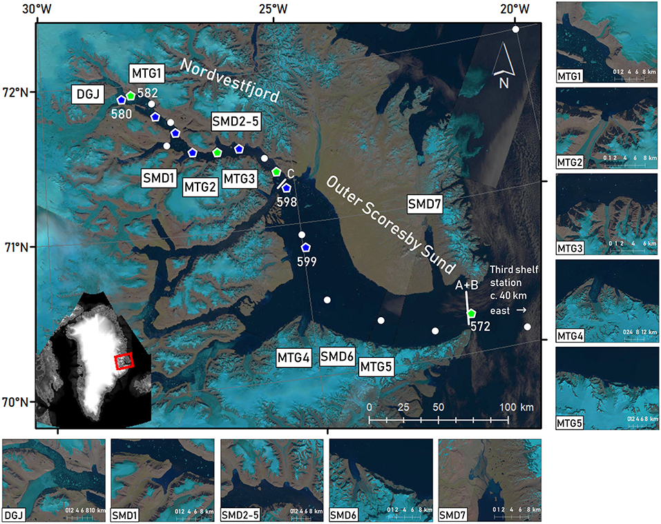
Figure 1. Landsat 8 false color images (OLI/TIRS C1 Level-1, courtesy of the U.S. Geological Survey) of the period of sampling (15 to 26 July 2016, depending on image availability and cloud cover), showing the Scoresby Sund fjord system and the fjord parts visited, namely Nordvestfjord and Outer Scoresby Sund (OSS). Light blue regions correspond to the ice cover of the GrIS. Major marine-terminating glaciers (MTG1-5) and surface meltwater discharges (SMD1-7) are marked in the map and displayed in enlarged images. Daugaard-Jensen glacier (DGJ) is indicated at the head of Nordvestfjord. White lines at the fjord mouth (A+B) and the entrance to Nordvestfjord (C) mark the positions of the LADCP transects during MSM76. Marks show sampling stations during MSM56, with green pentagons showing where sediment traps were deployed, and blue pentagons indicating where the camera profiles were performed. At the other stations (white circles), the standard sampling program was conducted, including CTD casts and in most cases sampling for nutrients and dissolved inorganic carbon/total alkalinity. Station numbers are included for stations that are explicitly mentioned in the text. Note that some stations were visited twice, upon entering and exiting the fjord system.

Daugaard-Jensen glacier at Nordvestfjord's head is a prominent marine-terminating glacier and the main generator of icebergs (Ó Cofaigh et al., 2001). The closest hydrographic station to the glacier terminus was situated 8–10 km away. Other large marine-terminating glaciers as well as major surface meltwater runoff pathways were identified by visual inspection of Landsat satellite images (USGS, EarthExplorer, Landsat 8 OLI/TIRS C1 Level-1, Figure 1) collected during our occupation of the fjord. In addition to Daugaard-Jensen glacier, three marine-terminating glaciers drain into Nordvestfjord and two into the OSS, with front widths of 1–11 km. Seven meltwater rivers flow into Nordvestfjord and two into the OSS.

2.2. Sample Collection and Analysis

Data were collected during a comprehensive sampling program with the German research vessel RV Maria S. Merian (cruise MSM56) (Koch, 2016). Twenty-two stations were sampled between 10 and 19 July 2016 along a transect from the inner Nordvestfjord to the fjord mouth, and additional three stations at the Greenland shelf (Figure 1).

At each station a CTD (Conductivity-Temperature-Depth) probe (SBE11plus Deck Unit with SBE9 sensors, Sea-Bird Scientific) equipped with additional sensors recorded vertical profiles of temperature, salinity, turbidity (ECO-NTU, WET Labs, Sea-Bird Scientific), chlorophyll a fluorescence (ECO-AFL/FL, WET Labs, Sea-Bird Scientific), and dissolved oxygen (SBE43, Sea-Bird Scientific) (Friedrichs et al., 2017). If not denoted differently, we report in situ temperatures in °C. Water samples were drawn from a rosette sampler with 24 Niskin bottles from discrete depths during the up-cast. Dissolved oxygen samples were taken for sensor calibration at all stations, and measured onboard within 24 h using Winkler titration. Salinity samples were collected in glass bottles and measured in the home laboratory. Note that all salinities in this paper are given on practical salinity scale (determined by electrical conductivity of seawater). Samples for nutrients (phosphate, nitrate, silicate) were collected in 50 ml LDPE bottles and stored frozen until analysis in the home laboratory. Nutrient concentrations were determined by a spectrophotometric autoanalyzer (QuAAtro39, SEAL Analytical) using slightly modified standard methods (Kattner and Becker, 1991). The measurement precision was 0.3% (coefficient of variation). Calibration of the nutrient analyses was performed using certified reference material (NMIJ CRM 7602-a, Seawater for Nutrients, National Metrology Institute of Japan, Ibaraki, Japan). Water samples for the determination of dissolved inorganic carbon (DIC) and total alkalinity (TA) were collected in 300 ml borosilicate bottles, poisoned with mercuric chloride, sealed, and stored in a cool place and in the dark. Measurements of DIC and TA were conducted with a VINDTA 3C (Versatile INstrument for the Determination of Total inorganic carbon and titration Alkalinity, Marianda, Kiel) including a CO₂ coulometer CM5015 (UIC Inc.) in the home laboratory. DIC was determined at 10°C by coulometry (Johnson et al., 1993; Dickson et al., 2007) with a precision of 1.4 μmol kg⁻¹. TA was measured at 25°C by applying a Gran potentiometric titration (Gran, 1952) with a precision of 1.8 μmol kg⁻¹. The methods were calibrated using certified reference material (batches #102 and #161) supplied by Scripps Institution of Oceanography, USA.

We used free-drifting surface tethered sediment traps to measure export flux at 100, 200, and 400 m depth for 5–10 h (Figure 1). The drifting traps consisted of a single drifting array with a surface buoy equipped with a GPS satellite transmitter, 12 small buoyancy balls serving as wave breakers to reduce the hydrodynamic effects on the sediment traps, and two 25 l glass buoyancy spheres. Each collection depth had four gimbal mounted collection cylinders, each 1 m tall and 10.4 cm in inner diameter. The collection cylinders were filled with filtered sea water with slightly increased salinity (4 permille increase) before deployment. The collected material was fixed with mercuric chloride and stored at 4°C until further analyses in the home laboratory. For the determination of the POC flux at the trap depths, samples were filtered on pre-combusted (450°C, 12 h) and pre-weighted Whatman GF/F filters (diameter: 25 mm) after removing swimmers, and dried for 48 h at 50°C. To remove particulate inorganic carbon, filters were fumed with 37% fuming hydrochloric acid for 24 h, dried for 24 h, and analyzed with a gas chromatograph (GC) elemental analyzer (EURO EA). In order to obtain discrete estimates of the POC flux in g C m⁻² d⁻¹ at the depths of the trap deployments, the weight of POC in a sample was divided by the area of the trap opening and the deployment time of the traps. For the determination of continuous POC flux profiles based on the discrete POC flux estimates of the sediment traps, we conducted optical recordings of vertical profiles at 12 stations using an in situ camera system (Figure 1). The custom camera system was self-constructed at AWI/MARUM and equipped with an infrared camera (acA2010-25gc GigE camera, Basler), an Edmund Optics compact fixed focal length lens 25 mm (#67-715) with aperture F#16, and an infrared light source. Every 500 ms (equivalent to a 15 cm depth interval), one picture was taken covering a volume of 20.46 cm³. The pictures were analyzed for particle size distribution and abundance by image processing using the image processing toolbox in Matlab R2015a (The MathWorks, Inc., Natick, MA, USA), following the method of Iversen et al. (2010) (see section 2.3). POC fluxes obtained from sediment trap deployments were used to fit the particle masses and sinking velocities (Iversen et al., 2010).

A HyperPro II profiling system (Satlantic, Canada) was used to acquire underwater light field information at selected stations depending on sea, weather, and daylight conditions, following procedures from Holinde and Zielinski (2016). Hyperspectral Ed(λ) data were then processed with ProSoft v.7.7.16 (Satlantic) and binned to 1 m depth intervals to calculate photosynthetically active radiation (PAR). Based on PAR(z), the 1% depth of PAR (a common indicator for the depth of the euphotic zone) was derived following Richlen et al. (2016), where PAR(0 m) data was extrapolated from the top 5 measurements.

In order to put the observed hydrographic and biogeochemical distributions into the context of ocean circulation, we analyzed direct velocity observations. Because they were not available from the cruise MSM56 in summer 2016, we use data that were obtained during the RV Maria S. Merian expedition MSM76 in summer 2018. This cruise was later in the year (11 August to 11 September 2018), but we believe that summer conditions, including the melting of marine- and land-terminating glaciers, led to similar circulation patterns as during the cruise MSM56 2 years earlier. Two meridional CTD and LADCP sections were carried out across the mouth of Scoresby Sound (sections A and B; see section Figure 1) from coast-to-coast, each comprising six stations. The work on section A started in the late afternoon, while section B was occupied 30 h later. Both sections were accomplished within roughly 7 h. In addition, one section consisting of four stations was carried out from coast-to-coast across the transition between the OSS and Nordvestfjord (section C; see Figure 1).

Regarding marine-terminating glaciers, the resolution of our dataset does not allow to distinguish between subglacial discharge (surface melt that is discharged through channels at the glacier base) and submarine melt (meltwater from below sea level) (Straneo and Cenedese, 2015). We therefore use both terms synonymously, even if we are aware that both meltwater types might enter the fjord waters in different ways.

2.3. Data Compilation

To assess the productivity of the fjord system, we calculated the net community production (NCP), which is defined as the gross primary production minus all losses in carbon due to respiration. It is used as a measure for the fraction of primary production that will be exported out of the surface layer, i.e., export production (Williams, 1993; Hansell and Carlson, 1998; Lee, 2001). NCP quantifies all biological activity that has occurred since ice break-up in spring until the time of sampling. While there are different methods to determine NCP (e.g., Hansell and Carlson, 1998; Bates et al., 2005; Munro et al., 2015), we utilize the difference in nutrients (particularly nitrate+nitrite and phosphate) between the winter and the time of sampling (Hoppema et al., 2007; Ulfsbo et al., 2014). In the high-latitude oceans and thus also in fjords, a remnant layer from the previous winter occurs below the seasonally heated surface layer. In this layer, nutrient concentrations are found as in winter (though sampled in summer). The winter remnant layer is defined by a temperature minimum below the seasonal halocline, and therefore kept out of contact with the atmosphere (Rudels et al., 1996; Hoppema et al., 2000, 2007; Ulfsbo et al., 2014). Because local vertical mixing had modified the temperature minimum to some extent, resulting in variability of the nutrient concentrations, we used the mean nutrient concentration of the Polar Water on the shelf (see definition of this water mass in section 3); here we assume that this is the main subsurface water source to the fjord and its residence time is more than 1 year. The temperature and salinity sections (Figures 4A,B) appear to confirm the Polar Water to be this source. Mean concentrations in the Polar Water at three shelf stations were 6.3 ± 1.3 μmol l⁻¹ for nitrate+nitrite, and 0.6 ± 0.09 μmol l⁻¹ for phosphate. For the depth of the winter remnant layer we took the temperature minima at the individual stations (between 41 and 135 m depth).

The net nutrient drawdown was obtained at each station by integrating the difference between the concentration in the temperature minimum and that in the surface layer above it. To exclude dilution by ice melt, evaporation, and precipitation, nutrient concentrations were normalized to a constant salinity of 34.5, as described in Hoppema et al. (2007). We then applied the following equation (modified after Ulfsbo et al., 2014):

$\begin{array}{ll}NC{P}_x[mmolC{m}^{-2}perio{d}^{-1}]={\displaystyle {\int }_0^{T_{min}}(X_{initial}-X_{measured})}dz·R_{C/X},& (1)\end{array}$

where X represents the nutrient concentration, either initial in the winter remnant layer, or measured at each sampling depth. R_C/X is the stoichiometric nutrient ratio which is necessary to convert nutrient units to carbon units. In this study we use the canonical Redfield ratio of 106C:16N:1P (Redfield et al., 1963). The integration was performed by linear interpolations between nearest sampling depths. In Young Sound, primary production below sea-ice was negligible because of a thick snow cover and active sea-ice melt which limited sea-ice-related production rates to 1 month or less (Glud et al., 2007). Based on this, we assumed that biological production in Scoresby Sund started with ice break-up (which we identified using satellite images), and could then calculate the daily NCP. The dates of ice break-up, the number of open water days until sampling, and the NCP based on nitrate+nitrite and phosphate deficits at each station are listed in Table 1. Upwelling of nutrients from depth can result in an underestimation of the NCP. However, upwelling during summer in Scoresby Sund does not fuel the whole surface layer (see section 4.2.1). Hence, we believe that it does not severely affect primary production and, thus, the production estimate based on nutrient deficits. NCP estimates can fluctuate depending on the assumptions made during the computation process. The main assumptions in the calculation of NCP are: (1) The source water is the Polar Water from the shelf near the mouth of Scoresby Sund; the source concentrations of nutrients may have been changed during transfer through the fjord system, both laterally and vertically. Since the Polar Water is vertically separated from its neighboring water masses by strong gradients, little exchange will likely occur with these during its transfer through the fjord. For the same reason, the vertical exchange at the stations is thought to be relatively small. (2) Homogeneity of the water column during winter and negligible winter draw-down of nutrients; in other fjords, winter draw-down has been observed, although not in all fjords (Glud et al., 2007); this may lead to a slight underestimation of the computed NCP. Accounting for variability in our definition of winter nutrient concentrations resulted in deviations in our estimates of NCP of ±18% (from nitrate+nitrite deficits) and ±41% (from phosphate deficits) from the ones presented here.

TABLE 1

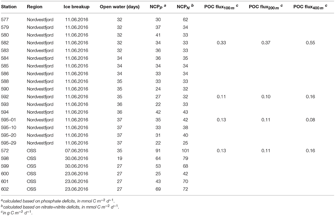
Table 1. Time of ice breakup, NCP (based on nitrate+nitrite, and phosphate), and flux of particulate organic carbon measured in sediment trap samples per station (stations with only CTD and shelf stations casts are not included). At station 595, four sampling rounds were conducted within 24 h.

Figure 2 presents the total aggregate volume and the POC flux throughout the water column as estimated from camera images. In the following, we use the term “particles" to refer to aggregates of inorganic and dead organic material and fecal pellets, while the POC flux only comprises the mass flux of organic carbon that is incorporated in the particles. Particle abundance and size were recognized using an image analyzing tool (medfilt2 function in Matlab R2015a) after converting the pictures into binary files and correcting them for background disturbance, such as shadows from illumination artifacts and spots on the camera lens. The pixel number of each projected particle area was determined and converted into equivalent spherical diameter (ESD) using the pixel to mm ratio. Detected particles were sorted into 20 logarithmically spaced size bins (d) based on their ESDs, ranging from 20 to 3415.03 μm. Each picture was concatenated to its respective in situ depth. Knowing the volume of the water cell pictured by the camera, the number of particles per liter and size class could be calculated (ΔC), and from it the total particle volume (Figure 2A). To account for statistical relevance, especially for the sparse large particles, we binned 10 consecutive pictures and only included size bins that contained five or more aggregates. In order to calculate the particle size distribution n, the number of particles per liter in a given size class was divided by the size difference between the concomitant size classes, as described by Iversen et al. (2010). As the POC flux within a certain time period was estimated from sediment traps that were deployed at three depths in the water column, a time dimension and POC estimate could be given to the particle volume (Figure 2B). For this, the total POC flux F was assumed to be an integration of the mass flux spectra of all particle sizes (modified after Iversen et al., 2010):

$\begin{array}{ll}F={\displaystyle {\int }_{sizeclass1}^{sizeclass20}n(d)·m(d)·w(d)·d(d),}& (2)\end{array}$

where n (#m⁻³cm⁻¹) is the particle size distribution in a given small size range, d(d), m is the particle mass (as POC), and w (md⁻¹) is the average sinking velocity of the particles in a given small size range, d(d). While n and d are known, m and w have to be determined. Since both particle mass m and sinking velocity w scales as a power relationship when expressed as a function of particle diameter d, the product of m and w also scale as a power relationship as a function of d. We used a minimization procedure to find the factor and exponent providing the best-fit between the trap collected fluxes and F obtained from the in-situ images at the trap depths, using the Matlab R2015a function fminsearch.

FIGURE 2

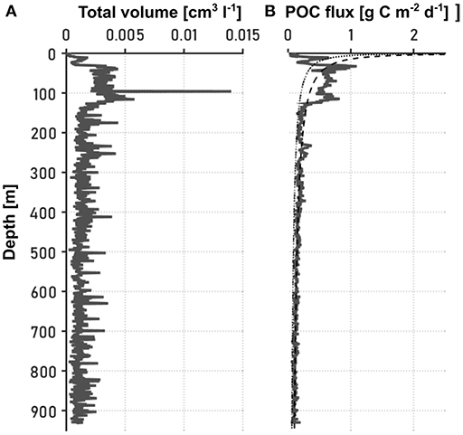
Figure 2. Vertical distribution of the (A) total particle volume [cm³l⁻¹], and (B) POC flux [g C m²d⁻¹]. An artifact on a picture at 100 m depth lead to a single high value in (A), but by relating the sediment trap POC measure during the computation process to all pictures within a depth range of 10 m above and below the actual depth of the sediment trap, this artifact was removed in (B). The dotted line in (B) indicates the Martin curve based on the maximum and the deepest POC fluxes. For the dashed line in (B), the remineralization exponent b from the previous fitting as well as the NCP at the surface were used.

As most of the camera profiles did not cover the water column down to the bottom, we fitted a Martin curve to the profiles for extrapolation (Martin et al., 1987; Belcher et al., 2016):

$\begin{array}{ll}F(z)=F(z_0)·{(z/z_0)}^{-b},& (3)\end{array}$

where F is the POC flux at depths z₀ and z, and b is the remineralization exponent. This exponent can also be considered as efficiency with which carbon that is exported from the upper ocean, i.e., F(z₀), decreases with depth (Guidi et al., 2015). High b values indicate high degradation of organic matter, while negative b values show initially increasing POC flux with depth. From the camera profiles we obtained a b value for each station. By replacing F(z₀) by the NCP at each station and using the corresponding b value, the fraction of NCP potentially reaching the sea floor was determined (Figure 2B).

The Martin curves differ considerably from the POC flux profiles at the surface, which might be the result of small particles that could not be detected on the images. However, the general pattern of the decrease in POC flux is consistent: POC flux and total aggregate volume peak in the upper 100 m of the water column, and particles are attenuated to low and quasi constant fluxes at depths below 200 m. To test the robustness of the findings based on the b value with a more simple approximation of export and remineralization, we calculated the ratio between the discrete POC fluxes at 100 m depth and the NCP estimates at the camera stations (by relating sediment trap stations with the closest camera stations).

3. Results

On the shelf of east Greenland, Polar Water (PW) with a salinity (S) below 34, and temperature (T) near the surface freezing point—exported from the Arctic Ocean—is advected toward the south near the sea surface. Below the PW, a warm and saline water mass (T > 0°C) is found, referred to as Atlantic Water (AW). A warmer and more saline variety of AW originates from waters recirculating in Fram Strait, while a slightly colder and fresher AW type is exported from the Arctic Ocean (Rudels et al., 2002). The characteristics of PW and AW are well-reflected by the water masses in OSS (Figures 3A, 4A,B), with PW found approximately above 200 m. Specifically, pronounced PW properties with temperatures below -1.4°C are observed at depths shallower than 150 m. Within the AW layer, found approximately below 200 m, salinity increases toward the bottom, while there is a temperature maximum near 1.2°C well-above the sea floor and a temperature minimum of T <0.7°C at the bottom (Figures 4A,B). In addition, above the PW a ~10 m thick very fresh surface layer was recorded, with temperatures sometimes exceeding 3°C, most likely reflecting summertime surface discharge of meltwater from the GrIS combined with solar heating in the fjord. As a result, maximum mixed layer depths are limited to the upper 10 m of the water column. During the cruise we noticed the presence of icebergs from calving glaciers in the whole fjord with increasing density toward the fjord head.

FIGURE 3

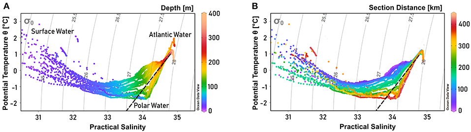
Figure 3. Temperature-salinity diagram of Scoresby Sund, showing the primary water masses present in the study area (after Rudels et al., 2002). Colors indicate (A) depth and (B) section distance, while gray lines indicate isopycnals. The dashed black line represents the Gade line between the Atlantic Water (T = 1 °C, S = 34.8) and the meltwater endmember of glacier termini (T = –90 °C, S = 0). One station with a distinct Atlantic Water signal was not included in the section profiles, as it was further north on the Greenland shelf. It is therefore visible in (A), but not in (B). Potential temperature was derived from in situ temperature using Ocean Data View 4 software (Schlitzer, 2004).

FIGURE 4

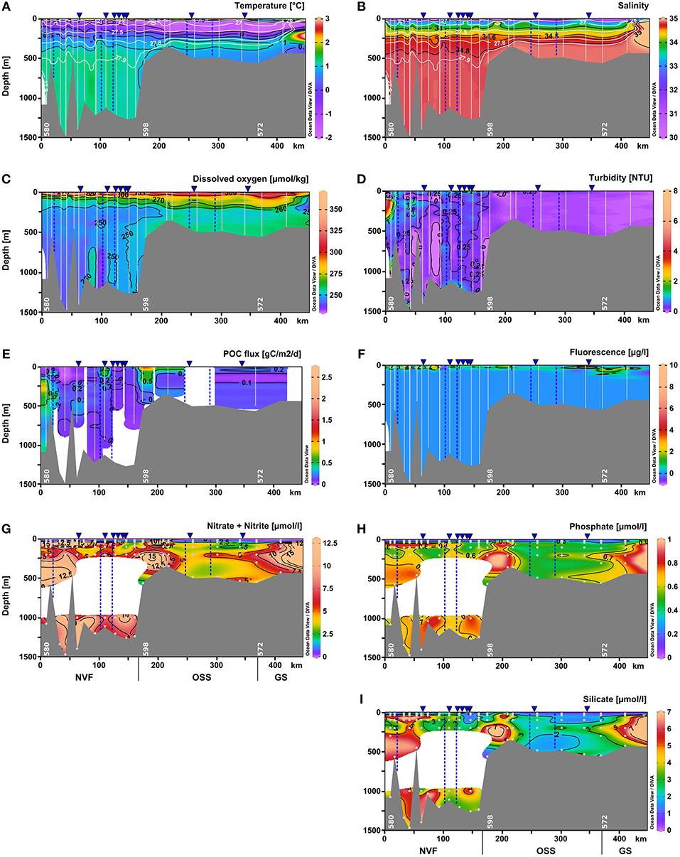
Figure 4. Vertical distribution of (A) temperature (°C), (B) salinity, (C) dissolved oxygen (μmol kg⁻¹), (D) turbidity (NTU), (E) POC flux (g C m⁻² d⁻¹), (F) chlorophyll a fluorescence (μg l⁻¹), (G) nitrate+nitrite (μmol l⁻¹), (H) phosphate (μmol l⁻¹), and (I) silicate (μmol l⁻¹) as distance from the fjord head (left) to the shelf (right) using Ocean Data View 4 software (Schlitzer, 2004). Data were interpolated by DIVA gridding, or for the POC fluxes by weighted-average gridding due to the low profile number. Bright lines indicate the CTD and camera profiles, bright dots represent water samples. The approximate positions of marine-terminating glaciers are shown by blue dashed lines, and surface meltwater discharge by blue triangles above the panels. Daugaard-Jensen glacier is situated close to the westernmost station (left side of the panels). NVF is the acronym for Nordvestfjord, OSS stands for the Outer Scoresby Sund, and GS for the Greenland Shelf.

Hydrographic properties change along the fjord axis from the mouth toward the inner part of Nordvestfjord. At depths below 400 m, the entire Nordvestfjord is filled by AW with temperatures exceeding 1.1°C (Figure 4A). This indicates that the sill separating the OSS and Nordvestfjord only allows for the warmer and less dense AW fraction to flow from the OSS into Nordvestfjord, while the colder AW bottom layer is held back. While the AW temperature maximum remains largely unchanged throughout the fjord system all the way into inner Nordvestfjord, the subsurface waters above the AW layer experience substantial warming with increasing distance from the mouth. As can be seen from Figures 3A, 5A,B temperatures are higher than –1.0°C in this layer in Nordvestfjord, even up to 0.5°C. Consequently, the steep transition in T/S space from PW to the AW temperature maximum present at the mouth of Scoresby Sound is observed to level off toward the inner fjord with the sill toward Nordvestfjord marking at particularly pronounced transition in T/S space around the 27.5 kg m⁻³ isopycnal (Figure 3B). At the same time, the 27.9 kg m⁻³ isopycnal deepens from 300 m in the OSS to 500 m in Nordvestfjord, indicating higher densities (salinities) to be present in the OSS compared to Nordvestfjord in this depth range. This pattern is reminiscent of a deep overflow (spill) of AW across the sill that, however, does not extend all the way to the bottom in Nordvestfjord.

FIGURE 5

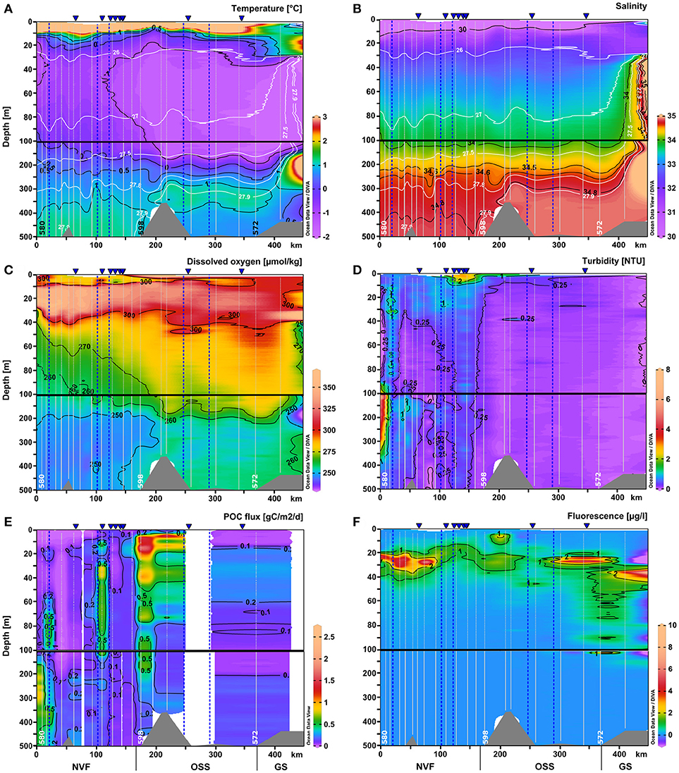
Figure 5. Same as Figure 4 for the upper 500 m of the water column: (A) temperature (°C), (B) salinity, (C) dissolved oxygen (μmol kg-1), (D) turbidity (NTU), (E) POC flux (g C m-2 d-1), and (F) chlorophyll a fluorescence (μg l-1). Section plots of the nutrient distributions are in Figure 6. The scale of the upper 100 m was expanded.

Dissolved oxygen concentrations were lowest in the deep basin (> 700 m), reaching ~240 μmol kg⁻¹. In Nordvestfjord between 10 and 30 m depth, the highest dissolved oxygen concentrations were found reaching 350 μmol kg⁻¹ and in the OSS in the same depth range these values decreased to 320 μmol kg⁻¹. In the upper 10 m of the water column of the OSS, dissolved oxygen concentrations were much lower reaching 280 μmol kg⁻¹, but increased to 300 μmol kg⁻¹ toward the fjord mouth (Figures 4C, 5C).

The surface water nutrients in the upper 25 to 50 m were largely depleted, with concentrations of about 0.1, 0.2, and 1.2 μmol l⁻¹ for nitrate+nitrite, phosphate, and silicate, respectively (Figure 6). An exception was a region at 120–150 km section distance characterized by high surface meltwater discharge (Figure 1, SMD2-5) where silicate concentrations reached up to 6.0–6.1 μmol l⁻¹, which is 2–3 times higher than in the surface layer at all other stations (Figure 6C). No other nutrient had such elevated concentrations here and also chlorophyll a fluorescence did not show a maximum. Between 20 and 30 m depth, chlorophyll a fluorescence was high with maximum values of up to 6.6 μg l⁻¹ at the innermost stations (0–100 km section distance), but decreased considerably to about 1.4 μg l⁻¹ at a section distance of 100 km and further toward the transition to the OSS (Figures 4F and 5F). Beneath 30 m depth, nutrient concentrations were significant but not homogeneously high within the water column of Nordvestfjord. The OSS was supplied by nutrients from the Greenland shelf that were transported within PW and AW at depths from 40 m to the bottom with concentrations of up to 12 μmol l⁻¹ for nitrate+nitrite, 0.8 μmol l⁻¹ for phosphate, and 6.0 μmol l⁻¹ for silicate. These concentrations decreased toward the sill to Nordvestfjord (Figures 4G–I). Chlorophyll a fluorescence was high with maximum values of 9.8 μg l⁻¹ within a layer at 25–50 m depth (Figure 5F).

FIGURE 6

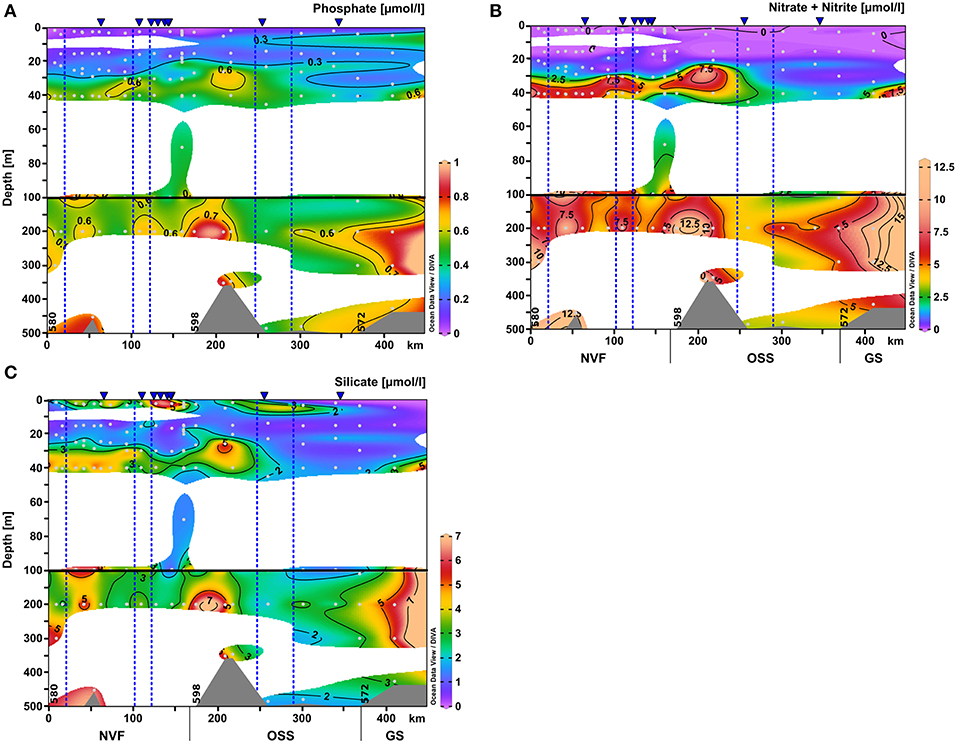
Figure 6. Same as Figure 4 for the nutrient distributions within upper 500 m of the water column: (A) nitrate+nitrite (μmol l-1), (B) phosphate (μmol l-1), and (C) silicate (μmol l-1). The scale of the upper 100 m was expanded.

Two patches of high chlorophyll a fluorescence in the OSS with 1.2 and 9.8 μg l⁻¹ correlated with patches of high dissolved oxygen concentrations (301.5 and 302.4 μmol kg⁻¹) and high turbidity (0.14 and 0.35 NTU) at 46 and 27 m depth and 260 and 300–340 km section distance, respectively (Figures 5C,D,F). Otherwise, turbidity was low in the OSS with about 0.09 NTU compared to Nordvestfjord with 0.3–0.5 NTU and a throughout turbid water column (Figure 4D). Highest turbidity in the Nordvestfjord was found at 100–200 m depth at the station closest to Daugaard-Jensen glacier, with a maximum of 3.8 NTU at 120 m depth (Figure 5D). Besides, values close to the surface and to the bottom were elevated with 0.6–0.7 and 0.5–0.8 NTU, respectively. At 120–150 km section distance, surface turbidity was almost one order of magnitude higher than within large parts of the water column (2.2–2.9 NTU), coinciding with elevated silicate concentrations (Figures 5D, 6C).

The depth of the euphotic zone as derived from the 1% depth of PAR ranged between 20 and 69 m throughout the whole study area. While light penetration varied in the Nordvestfjord between 20 and 44 m (mean = 32 m, standard deviation = 7 m), it increased toward the OSS and the adjacent Greenland shelf, ranging from 34 to 69 m (mean = 48 m, standard deviation = 11 m).

DIC and TA correlate strongly with salinity (${\text{R}}_{DIC}^2$ = 0.906 and ${\text{R}}_{TA}^2$ = 0.942; n = 54 for DIC, n = 46 for TA) (Figures 7A,C). Normalization to a constant salinity of 34.5 revealed that low-salinity samples (mainly surface samples of Nordvestfjord) were profoundly affected by processes other than dilution (Figures 7B,D). They were therefore not taken into account for the extrapolation to zero salinity (i.e., representing meltwater discharge), which yields concentrations of 423 and 726 μmol kg⁻¹ for DIC and TA, respectively (Figures 7A,C). Note that these freshwater endmember concentrations were used for salinity normalization (Friis et al., 2003), but that assuming a freshwater endmember with zero concentrations of DIC and TA, respectively, resulted in the same trend for normalized low-salinity samples. Non-conservative changes in DIC can be caused by a number of processes, including uptake of atmospheric CO₂, remineralization, and photosynthesis. No clear trend could be identified in the normalized DIC values of low-salinity surface samples (Figure 7B), indicating an interaction of several processes. Non-conservative behavior of TA, by contrast, is mainly attributed to carbonate mineral precipitation and dissolution (e.g., Cross et al., 2013). As most low-salinity surface samples had lower normalized TA values than the samples with higher salinities (which display a conservative relationship between TA concentration and salinity) (Figure 7D), we assume that they reflect carbonate mineral precipitation.

FIGURE 7

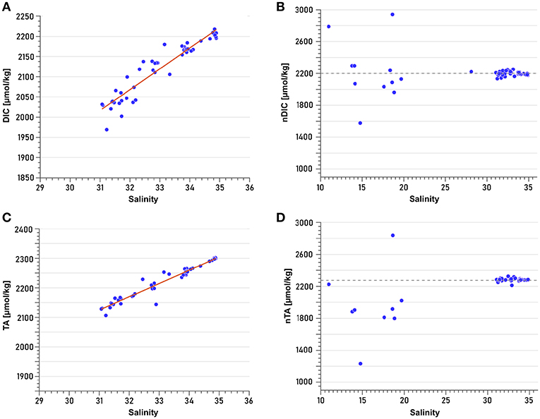
Figure 7. Least-square linear regressions of (A) Total dissolved inorganic carbon (DIC) vs. salinity (R² = 0.906) and (C) Total alkalinity (TA) vs. salinity (R² = 0.942). Linear regressions were performed based only on samples with salinities >25. Normalization of (B) DIC and (D) TA was performed according to the formula of Friis et al. (2003) for non-zero freshwater endmembers. Dashed lines in (B,D) represent the approximate mean values of the samples with salinities >25. Deviations relative to this line (low-salinity samples, mainly from the surface of Nordvestfjord) indicate processes other than conservative mixing that modify TA and DIC concentrations.

The NCP was high in the OSS (58 mmol C m⁻² d⁻¹ for phosphate deficits, 82 mmol C m⁻² d⁻¹ for nitrate+nitrite deficits) compared to Nordvestfjord (32 mmol C m⁻² d⁻¹ for phosphate deficits, 36 mmol C m⁻² d⁻¹ for nitrate+nitrite deficits; Table 2). Visual analyses of net samples from Nordvestfjord revealed that the phytoplankton community was already in a post-bloom stage (B. Edvardsen, personal communication). Much debris, many copepods, and fecal pellets found in the sediment traps show that intense grazing already diminished the primary production. By contrast, a healthy and thriving phytoplankton community was observed in net samples of the OSS.

TABLE 2

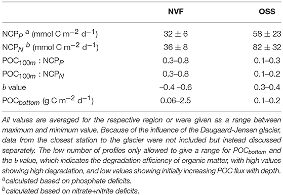
Table 2. Production, carbon flux, and remineralization in Nordvestfjord (NVF) and the Outer Scoresby Sund (OSS).

Camera-derived POC fluxes in Nordvestfjord and at the innermost part of OSS were high close to glacier fronts, ranging from 0.5–2 g C m⁻² d⁻¹, and lower in the remaining Nordvestfjord (0.1–0.3 g C m⁻² d⁻¹; Figure 4E). In the OSS, they decreased with increasing depth within the surface layer and corresponded well with the stratification of the water masses below (0.1–0.2 g C m⁻² d⁻¹). It has to be noted that only one POC flux profile is available for the OSS and none for the shelf. The b value, constituting the remineralization efficiency, is higher in the OSS (0.3–0.4) than in Nordvestfjord (–0.4–0.6), indicating that a smaller share of the surface production in the OSS is transported to depth. The POC_100m : NCP ratio confirms this, showing that the POC flux at the depth of the shallowest sediment trap at 100 m makes up only 10–20 or 10–30% (for NCP_N and NCP_P, respectively) of the surface production in the OSS, while in Nordvestfjord, 30–80% of the NCP (both, NCP_N and NCP_P) are reflected in the POC flux at 100 m depth. According to the Martin curve, between 0.06 and 2.5 g C m⁻² d⁻¹ of POC reached the sea floor in Nordvestfjord, which is more than the average amount fixed per day by primary production since the start of the growing season, whereas only 5–15% of the NCP in the OSS was sedimented on the seafloor (0.1–0.2 g C m⁻² d⁻¹) (Table 2).

Traces of the pronounced freshwater discharge of Daugaard-Jensen glacier were detectable 8-10 km away from the glacier front at our station closest to the terminus (station 580). In order to highlight the impact of Daugaard-Jensen's meltwater discharge on biogeochemical cycling in Scoresby Sund, we contrast measurements at two other stations (station 582 which is ~7 km further north of station 580, and station 599 in the OSS) in the same way as for station 580 (Figure 8). While at other stations at 200–240 m depth, salinity smoothly decreased with depth (examples given in Figures 8B,C), a sudden salinity drop by 0.1–0.2 units could be detected at station 580 (Figure 8A). The temperature-salinity diagram reveals a salinity-driven density decrease, indicated by an approximately horizontal line compared to the stations 582 and 599 (Figure 8D). At station 580, nutrient concentrations were reduced by one third at 100–200 m depth compared to nutrient concentrations at 300 m depth. At 40–100 m depth nutrient concentrations were slightly higher. A reversed pattern was observed for turbidity, with a maximum at 100–200 m depth (2.5–3.9 NTU) and lower turbidity in the water masses above 100 m and below 200–250 m at this station. NCP, reaching 41 and 33 mmol C m⁻² d⁻¹ (for phosphate and nitrate+nitrite deficits, respectively), was not considerably higher compared to NCP at other stations (Table 1), but the POC flux was elevated at 250–350 m depth (up to 1 g C m⁻² d⁻¹) and with 4.0–4.9 g C m⁻² d⁻¹ (b value: -0.57) the sedimentation rate to the bottom was higher next to the glacier (station 580) than in the remaining Nordvestfjord. Maximum nutrient concentrations at the next station further outfjord (station 582) were measured at 100 m depth, coinciding with a POC flux maximum of 0.8 g C m⁻² d⁻¹. Turbidity was higher within the upper 250 m (~1 NTU) than below (~0.5 NTU). At a station within the shallower OSS (station 599), nutrient concentrations were increasing from the surface up to a depth of 50 m, which coincides with an elevated POC flux (up to 0.4 g C m⁻² d⁻¹), high turbidity (1.5–3.0 NTU), and high chlorophyll a fluorescence (Figure 5F), indicating active primary production and remineralization. Below, nutrient concentrations and turbidity increased toward the depth of the AW (200 m), while the POC flux stayed low throughout the water column.

FIGURE 8

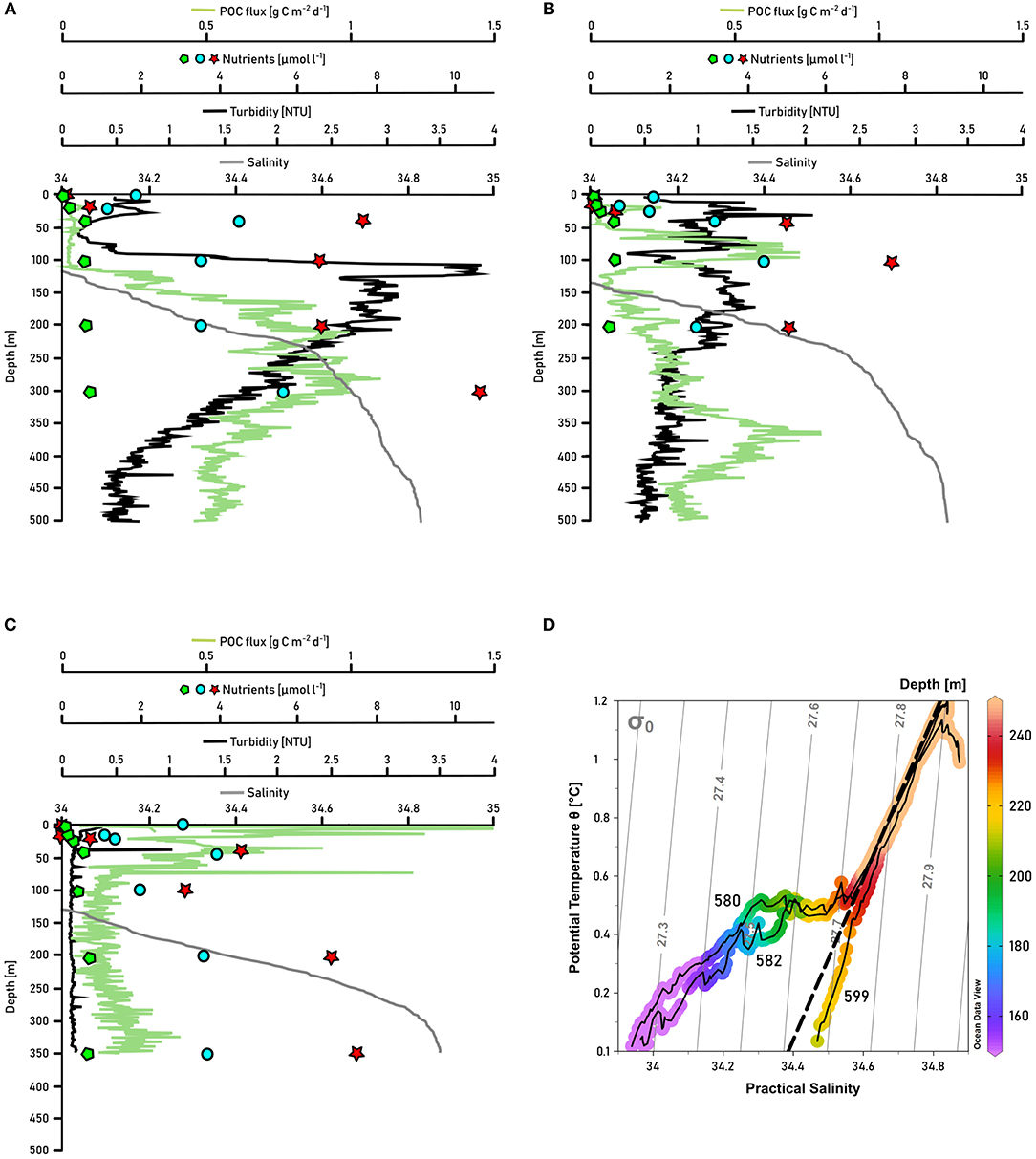
Figure 8. Salinity (gray line), turbidity (black line), POC flux (green line), nitrate+nitrite concentrations (red stars), silicate concentration (blue dots), and phosphate concentration (green pentagons) in the upper 500 m of the water column of the stations (A) 580, which is closest to the glacier front of Daugaard-Jensen glacier, (B) 582, which is next to 580, but a bit further outfjord, and (C) 599, a station in the middle of OSS. (D) displays the temperature-salinity diagrams of the three stations, colormarked for depths. Gray lines indicate isopycnals, the dashed black line represents the Gade line between the Atlantic Water (T = 1 °C, S = 34.8) and the meltwater endmember of glacier termini (T = –90 °C, S = 0). Potential temperature was derived from in situ temperature using Ocean Data View 4 software (Schlitzer, 2004).

4. Discussion

Figure 11 summarizes the main processes that are discussed in the following chapters.

4.1. Circulation

The circulation of AW (i.e., temperatures exceeding 0°C) at the fjord mouth (sections A and B; see Figure 1) is characterized by an inflow of AW into Scoresby Sund at the northern part of the section and an outflow of AW in the southern part (Figure 9, upper panel). Thereby, the strongest flows are observed close to the northern and southern margins, suggesting boundary currents to be present along either margins. The observed circulation in the PW layer is considerably more patchy and weak overall (Figure 9, upper panel). In order to quantify the strength of the circulation, cumulative cross-section transports (integrated from north to south) have been computed for both sections A and B (Figure 9, lower panel). This has been done both based on the observed velocities (solid lines) and after a correction for barotropic tidal currents was applied (dashed lines). Despite differences between the 4 graphs, there is qualitative agreement in the sense that the inflow is found in the northern half of the section and outflow in the southern part. The maximum inflow lies between 110 and 190 · 10³ m³ s⁻¹ for the original data and reduces to values between 60 and 100 · 10³ m³ s⁻¹ after tidal correction (Figure 9, lower panel). Note that after tidal corrections for both sections there is a higher degree of compensation between inflow and outflow than without the correction (Figure 9, lower panel). As mass should be approximately conserved on weekly and long time scales, the tidal correction seems to add to the plausibility of the results.

FIGURE 9

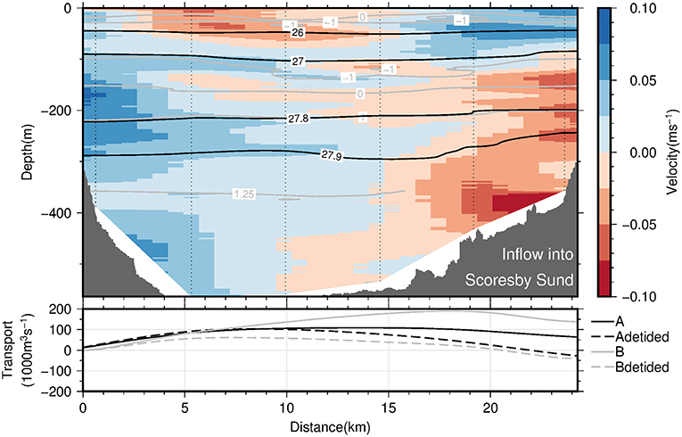
Figure 9. The (Upper panel) displays the across-section velocity profiles (vertical, dotted lines) (interpolated onto a regular grid using 2D-spline interpolation) along the mouth of Scoresby Sund as a function of both depth and along-section distance from northern section end point. The view is out-fjord directed. Blue shading denotes inflow of waters from the continental shelf into Scoresby Sund, while red shading denotes outflow. Also shown are selected isopycnals and isotherms as black and gray solid lines, respectively. The (Lower panel) displays the cumulative volume transport into Scoresby Sund (precisely, the meridional integral of the vertically integrated across-section velocity along the mouth of Scoresby Sund) as a function of along-section distance from the northern section end point. The transports based on the LADCP profiles from the sections A and B are displayed as solid black and gray lines, respectively. The corresponding dashed lines denote the same transport quantities computed after subtracting barotropic tidal velocities from the LADCP profiles as predicted by the AOTIM-5 inverse tide model (Padman and Erofeeva, 2004).

Section C across the transition between the OSS and Nordvestfjord (see Figures 1, 10, left panel) is divided into two 4 km-wide channels separated by an island in the middle. The location where the section was taken is placed beyond the sill (at a distance of ~180 km; Figure 4A) where the sea floor slopes downward into Nordvestfjord. Here, a pronounced, bottom intensified inflow of the warmest part of AW into Nordvestfjord at densities exceeding 27.9 kg m⁻³ (and T > 1.1°C) is found in both channels. This supports the fact that the deep part of Nordvestfjord is filled by AW with temperatures exceeding 1.0°C (Figure 4A). The outflow is found in both channels to occur mainly at middepths confined to a layer bounded by the 27.9 kg m⁻³ at the bottom and the 0°C isotherm (i.e., the AW-PW interface) at the top. At shallower depths, a weak flow toward the OSS is found. Overall, the flow across section C seems to vary strongly with depth, with an inflow of warm AW of 65 · 10³ m³ s⁻¹ at the bottom, compensated by an outflow of slightly colder AW. There is no indication of pronounced horizontal recirculation as was found at the mouth of Scoresby Sund.

FIGURE 10

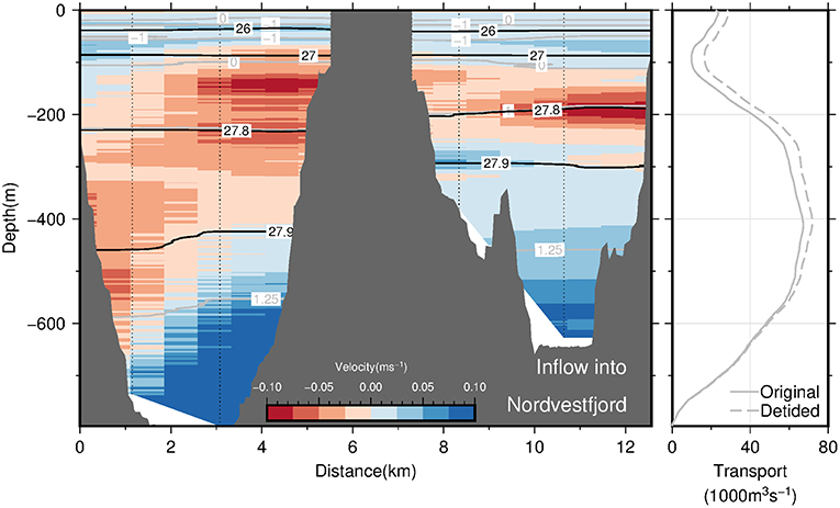
Figure 10. The (Left panel) displays the across-section velocity based on LADCP profiles (interpolated onto a regular grid using 2D-spline interpolation) at transition between the OSS and Nordvestfjord (section C) as a function of both depth and along-section distance. The view is in-fjord directed. Blue shading denotes inflow of waters from the OSS into Nordvestfjord, while red shading denotes outflow. Also shown are selected isopycnals and isotherms as black and gray solid lines, respectively. The black, solid line in the (Right panel) displays the cumulative volume transport into Nordvestfjord (precisely, the cumulative integral of the along-section integrated across-section velocity from the seafloor to the sea surface) as a function of depth. The transport is based on the LADCP profiles from section C. The corresponding dashed line denotes the same transport quantity computed after subtracting barotropic tidal velocities like in Figure 9.

In summary, our observations suggest the presence of boundary currents at the mouth of Scoresby Sund. At horizontal scales exceeding the baroclinic Rossby Radius of deformation, R_D, the Coriolis force is expected to impact the circulation such that boundary currents exist. Based on the hydrographic profiles, we estimated R_D to amount to 6 km (following Nurser and Bacon, 2014), both at the mouth of the OSS and near the sill toward Nordvestfjord. The OSS exhibits typical widths of 35 km and exceeds 25 km at the mouth. This means that a horizontal circulation patterns with boundary currents along either margin represents plausible features of the circulation which we expect to exist throughout the OSS. The sense of the circulation (inflow along the northern margin and outflow along the southern one) can be reconciled with the fact that the Coriolis force acts on the flow to the right relative to the flow direction. At the transition of the OSS to Nordvestfjord (Figure 10), where the fjord becomes narrow, no evidence for horizonal recirculations are found. Here the flow seems to vary mainly in the vertical - reminiscent of estuarine circulations with an inflow at depth and outflow above this.

The inflow of warm AW into Scoresby Sund at depth and the compensatory outflow at shallower levels means that the heat, salt, and mass need to be transported upward within Nordvestfjord. The gradual warming of the subsurface layer (erosion of PW layer) may be explained by this. The fact that the isohalines are essentially flat in the upper 200 m throughout the OSS and Nordvestfjord may mean that there is a balance between salt being mixed upward and the input of freshwater from marine terminating glaciers and icebergs into the subsurface waters of the fjord.

4.2. Opposing Biogeochemical Regimes in Nordvestfjord and Outer Scoresby Sund

4.2.1. Nutrients and Turbidity

While deep nutrient concentrations in Nordvestfjord were elevated, the surface layer (up to 25–40 m depth) exhibited low nutrient concentrations (Figures 4G–I). Chlorophyll a fluorescence showed a maximum within a layer at 20–30 m depth, with laterally decreasing values in this layer with distance to the fjord head (Figure 5F). A surface patch with high silicate concentrations and elevated turbidity was found at 120–150 km section distance where numerous meltwater rivers drain into the fjord (Figures 1, 5D, 6C). Since there was no patch of other high nutrients, and the chlorophyll a fluorescence was not elevated, the surface meltwater must have been the source of silicate and silt. We assume that surface meltwater rivers accumulated silicate during their way across the bedrock surface.

Previous studies are not consistent in the information about the nutrient content of GrIS meltwater. While silicate has indeed been found to be transported into the system by glacial meltwater (Meire et al., 2016a; Hawkings et al., 2017), the meltwater contribution to phosphate and nitrate is unclear. The GrIS has been suggested to be a nitrogen source to phytoplankton (Hawkings et al., 2015, 2016; Wadham et al., 2016; Lund-Hansen et al., 2018). A fraction of this nitrogen might, however, not be readily bioavailable because it is bound to particles (Hawkings et al., 2015, 2016).

The indirect impact of glacier meltwater discharge on the distribution of nutrients and the resulting productivity in the fjord depends on the meltwater source. Meire et al. (2017) described two possible patterns: a fjord dominated by marine-terminating glaciers is likely to be productive because of enhanced upwelling of nutrient-rich deep water induced by the deep meltwater plume (see also Kanna et al., 2018). By contrast, a fjord that is dominated by land-terminating glaciers discharges meltwater directly into the surface layer and is therefore characterized by low productivity because of enhanced stratification.

Nordvestfjord is influenced by both marine- and land-terminating glaciers. A third pattern besides the two described above seems to emerge here. Surface meltwater discharged into the fjord has formed a stable low-saline layer in the upper 10 m of the water column and below that the salinity increased only gradually. Also upwelling of nutrients due to meltwater release at greater depths seems to occur. Nutrient concentrations were high below 25–40 m depth, depending on the region. However, apparently they did not reach the surface layer above that. Because of the low surface layer chlorophyll a fluorescence at most stations, it is unlikely that such nutrients would have been consumed by primary production in the upper 10–25 m. While it appears that primary productivity in the innermost part of Nordvestfjord was still active, low chlorophyll a fluorescence values at stations further out (> 100 km section distance until the sill to the OSS) suggest a termination of the bloom. The latter is supported by observations of a post-bloom plankton community, many copepods and fecal pellets in net samples and sediment traps during our cruise. Critical whether meltwater plumes of marine-terminating glaciers reach the surface or not are the distance to the glacier termini, the strength of the ambient stratification, the volume of subglacial discharge, and the grounding line depths (Sciascia et al., 2013; Carroll et al., 2015; Hopwood et al., 2018). Even when not much is known about the marine-terminating glaciers in Scoresby Sund, it seems as if these factors produced plumes that obtained neutral buoyancy below the photic zone with only having a minor fertilizing effect on primary production. The depth of neutral buoyancy can be different for each marine-terminating glacier.

Within PW and AW, nutrients were transferred from the Greenland shelf to the OSS in the layer from 40 m to the bottom with concentrations of up to 12 μmol l⁻¹ of nitrate+nitrite; 0.8 μmol l⁻¹ of phosphate; and 6.0 μmol l⁻¹ of silicate. It seems as if these waters would not supply the whole Scoresby Sund with nutrients, because nutrient concentrations decrease shortly after entering the OSS. However, our stations were located at the southern side of the OSS entrance, and thus in the outflowing water (see section 4.1). If we would have sampled further north, the connection between the inner fjord waters and the shelf waters in terms of nutrient concentrations would possibly have been clear.

Above, we discussed why no nutrients arrived in the very surface layer (upper 10–20 m), resulting in a low primary productivity in Nordvestfjord. However, the situation with the nutrients supply to the euphotic zone is more complicated than this. The euphotic zone ranged from 20 to 44 m (see section 3). In a similar depth range of 20–35 m, the chlorophyll a fluorescence maxima were found (Figure 5F). Nutrient concentrations were clearly higher in the deeper waters (>30 m) than in the near-surface water. This constellation can be explained by upwelling of nutrients which are consumed by primary producers near the lower boundary of the euphotic zone, identified by a chlorophyll a fluorescence maximum. Thus, the deep maximum of chlorophyll a fluorescence in the fjord is very much influenced by the different, shallow and deep, meltwater inflows which in turn determine the nutrient availability.

The sources of bulk particulates in Nordvestfjord, measured as turbidity (Figure 4D), can clearly be identified. GrIS meltwater discharge at the surface and at depth increased turbidity, indicating that GrIS meltwater introduced particulate material. Indeed, GrIS can carry a high load of terrestrial lithogenic matter, which has the potential to limit primary productivity due to light attenuation (Murray et al., 2015; Arendt et al., 2016; Richlen et al., 2016). Moreover, redistribution of sediments and phytoplankton cells increased turbidity at the bottom and at the surface, respectively. In the OSS, by contrast, turbidity was solely elevated at high-oxygen patches near the surface, suggesting that only plankton itself increased turbidity.

Light penetration as described by euphotic zone depth was highest were turbidity was lowest and vice versa, ranging from 20 to 69 m throughout the Scoresby Sund. Holinde and Zielinski (2016) reported 1% depths of PAR ranging from 12 to 42 m for two fjord systems at the west coast of Greenland (Uummannaq Fjord and Vaigat-Disko Bay), influenced by suspended inorganic matter concentrations and phytoplankton abundance. Lund-Hansen et al. (2010) investigated the Kangerlussuaq fjord-type estuary, also situated at Greenland's west coast, reporting on light penetration depth from <1 m near a meltwater outlet to a typical range from 6 to 39 m in the main part, again correlated with the concentration of suspended inorganic matter.

4.2.2. Dissolved Inorganic Carbon and Total Alkalinity

Estimates of DIC and TA in freshwater derived from inner fjord observations of Scoresby Sund are high, reaching 423 and 726 μmol kg⁻¹, respectively. Other studies found lower freshwater endmember concentrations of about 60–160 μmol kg⁻¹ for DIC and 160 μmol kg⁻¹ for TA in Godthåbsfjord using similar methods (Rysgaard et al., 2012; Meire et al., 2015). The reasons for high DIC and TA concentrations in freshwater are numerous. Surface meltwater can take up atmospheric CO₂ by bubble intrusion. Moreover, it has been reported that rivers flowing through the GrIS take up dissolved CO₂ from basal ice, and release it to the ocean and the atmosphere. The origin of this CO₂ is attributed to either inorganic mechanisms such as refreezing, or microbial metabolism. Even though these fluxes seem to be minor compared to other sources of CO₂, they might strongly increase as soon as melting has reached basal ice (Ryu and Jacobson, 2012). With respect to TA, the source of meltwater is particularly important. Runoff from land-terminating glaciers carries higher TA concentrations due to stronger interaction with the bedrock than the meltwater from marine-terminating glaciers (Anderson et al., 2000; Brown, 2002; Reisdorph and Mathis, 2014; Pilcher et al., 2018). Because our TA freshwater endmember concentration was almost five times those obtained by Rysgaard et al. (2012) and Meire et al. (2015) in Godthåbsfjord, we suspect that the contribution of meltwater from land-terminating glaciers in Scoresby Sund is higher than in Godthåbsfjord. Note that there are some uncertainties in the approach of obtaining a freshwater endmember estimate for TA and DIC, because low-salinity samples have been excluded from the linear extrapolation as they might have been influenced by biological processes.

TA and DIC concentrations from samples with salinities >25 mainly changed conservatively with salinity (Figures 7B,D). However, normalization to a constant salinity revealed that samples from low-salinity surface waters of Nordvestfjord must have been subject to processes other than dilution, because they deviated from a constant concentration at a salinity of 34.5. The relationship between TA and salinity suggests that precipitation of carbonate minerals plays a role, as its concentration in almost all samples was lower than it would have been expected from conservative mixing only. Because only few calcifying plankton species were present, we hypothesize that inorganic calcium carbonate was formed within the brine channels of sea ice that was formed during winter, which decreases dissolved DIC and TA in the brine (Rysgaard et al., 2009; Jones et al., 2010). When the sea ice melts during spring and summer, the brine is released to the surface layer, lowering the TA concentration of the surface water. Strikingly, the concomitant trend in DIC was more diverse with likewise higher and lower normalized DIC concentrations compared to a conservative mixing behavior. This indicates not only a depletion (which would have been expected from brine release as the only factor apart from conservative mixing changing the carbonate system), but also increasing concentrations of DIC at the surface. This increase independent from changes in salinity at the surface can be the result of several processes. On the one hand, the termination of the bloom in Nordvestfjord (see section 4.2.3) might have enhanced remineralization processes. On the other hand, a flux of CO₂ from the atmosphere to the fjord's surface water would have had more time to change DIC concentrations in Nordvestfjord compared to the OSS, because ice break-up occurred a few days earlier (Table 1). Finally, rising meltwater plumes from submarine glacial discharge can bring up low-DIC waters (Meire et al., 2015). However, due to the stable freshwater surface layer and the distribution patterns of nutrients, which are indicating no upwelling to the surface, we believe that the latter is the least likely cause.

4.2.3. Net Community Production

We observed a higher NCP in the OSS (58–82 mmol C m⁻² d⁻¹) than in Nordvestfjord (32–36 mmol C m⁻² d⁻¹, Table 2). However, a healthy and thriving phytoplankton assemblage in net samples taken in the OSS indicates that primary production had not been terminated at the time of the cruise. Thus, the calculated NCP in the OSS does not include the entire yearly production, and is therefore an underestimation of the annual NCP. Note that NCP was lower at the innermost station of the OSS than at the station closest to the fjord mouth (64–79 mmol C m⁻² d⁻¹ at station 598 vs. 91–101 mmol C m⁻² d⁻¹ at station 572, Table 1). In Nordvestfjord on the other hand, visual analysis of net samples and the catchment of debris, copepods, and fecal pellets in the sediment traps demonstrated that production was terminated. In the case of Nordvestfjord, remineralization of part of the organic material after the productive period might have caused our NCP to be underestimated.

Even though chlorophyll a fluorescence was still high at the innermost stations of Nordvestfjord, low chlorophyll a fluorescence further out-fjord and a post-bloom phytoplankton community imply that primary production in Nordvestfjord had largely come to an end. Thus, annual NCP was less than half of that in the OSS. Sealing of nutrients at greater depths was observed in Young Sound (Rysgaard and Nielsen, 2006), resulting in lower phytoplankton biomass compared to areas with less meltwater discharge (Middelbo et al., 2018). In addition, silts contained in the meltwater tend to limit production by decreasing the light penetration in the water column (Murray et al., 2015; Arendt et al., 2016). For the computation of the NCP we assumed little vertical or lateral mixing which could add nutrients from adjacent water masses; homogeneity of the water column during winter; a depletion of nutrients within a realistic time frame, and a negligible winter drawdown (Jennings et al., 1984; Hoppema et al., 2007). Because these assumptions may not completely hold in a fjord system, our computed NCP may be underestimated. In contrast, an overestimation of NCP may have been introduced at some locations in the OSS where we sampled on the southern side of the fjord and, thus, in the outflowing, nutrient-poor water (see section 4.1 and 4.2.1).

The difference in the timing of the blooms (post-bloom situation in Nordvestfjord vs. active bloom in the OSS) could have been triggered by an earlier sea ice retreat in Nordvestfjord by 12–19 days compared to the OSS. While in the OSS we sampled only 19–27 days after ice break-up (except for the outermost station 572 with 35 days), it was 32–37 days in Nordvestfjord (Table 1). Meire et al. (2016b) suggest that the intensity and location of the spring bloom in the southwest Greenland Godthåbsfjord is not only controlled by the presence of sea ice, but also by the upwelling of nutrient-rich water and wind forcing. Upwelling of nutrients seems to play a role in Scoresby Sund (see section 4.2.1), but the role of wind forcing is unclear, though it might be relevant in determining the timing of the blooms. Interestingly, the earlier bloom in Nordvestfjord compared to the OSS does not tally with observations in Godthåbsfjord, where the bloom in the inner fjord occurs later than further out-fjord (Hopwood et al., 2016; Meire et al., 2016b). According to a 2D-hydrodynamic model, the establishment of the ice cover in the northeast Greenland fjord Young Sound largely depends on tides and the related current velocities (Rysgaard et al., 2003), generating openings (polynyas and leads) in the sea ice during winter. We conjecture that also the ice break-up is affected by tidal dynamics. Hence, current velocities resulting from tides, and wind forcing may have acted differently on the winter sea ice cover in Scoresby Sund and in Godthåbsfjord, ending up in different timing of the blooms from the fjord mouths to the inner fjords.

From the snapshot that we made from Scoresby Sund's primary production it is difficult to use the terms “bloom” and “post-bloom” in a strict sense, because actual bloom dynamics over the course of a year would need to be examined further. We therefore use these terms in a broader sense, referring to active and recently terminated phytoplankton growth, respectively. Juul-Pedersen et al. (2015) described two phytoplankton blooms every year in Godthåbsfjord, a spring bloom in April/May and a summer bloom in July that was probably initiated by upwelling of nutrients from deeper layers. We could not observe such an upwelling of nutrients to the upper surface layer during the time of the expedition, but upwelling to the lower bound of the euphotic layer could be deduced from the existence of a maximum of chlorophyll a fluorescence. In the OSS, the import of nutrients from the shelf could have either supported a prolonged spring bloom or initiated a summer bloom. Our dataset does not allow further analysis of the temporal bloom dynamics in Scoresby Sund.

In the OSS, highest NCP values were observed at the fjord mouth, where primary producers were probably fed by nutrients from the PW and AW. High primary productivity along the shelf of Greenland sustains a high secondary production, and last but not least Greenland's export income due to efficient halibut landings (Meire et al., 2017). Estimates of NCP, especially in Arctic fjord and shelf regions which can be compared to our values in terms of methodology, are scarce. In Glacier Bay, Alaska, similar production rates as in the OSS of 54–81 mmol C m⁻² d⁻¹ were observed (Reisdorph and Mathis, 2015). Arrigo and van Dijken (2015) observed a decline in net primary production (derived by satellite chlorophyll a measurements, sea surface temperature, and sea ice cover) by 15% in the Greenland Sea between 1998 and 2012. The reasons for this are unclear, but an increase in productivity at the Scoresby Sund mouth seems unlikely. Shelf areas of the Chukchi Sea and the Larsen Shelf (Antarctica) that are both influenced by meltwater discharges are with 80–250 mmol C m⁻² d⁻¹ more productive than the OSS at the time of the cruise (Hoppema et al., 2000; Bates et al., 2005; Mathis et al., 2009). The reason for higher NCP in those latter regions may be that their growing season had been progressed further at the time of sampling relative to the growing season in the OSS. Thus, the NCP summed up over an entire year might be similar in Scoresby Sund compared to the other regions. Open water areas of polar regions, like the basin of the Chukchi Sea, the Arctic Ocean basin, and the Weddell Sea and Drake Passage in Antarctica, generally experience 10–100 times lower export production rates (Hoppema et al., 2000, 2007; Anderson et al., 2003; Bates et al., 2005; Mathis et al., 2009; Munro et al., 2015).

Differences in NCP estimates based on nitrate+nitrite or phosphate deficits may be a result of a deviation from the canonical Redfield ratio. This deviation may be caused by different remineralization rates of the nutrients, or a phytoplankton assemblage with a non-Redfieldian stoichiometric ratio. Also, nitrate is more prone to be altered by additional processes other than phytoplankton growth, for instance denitrification and nitrogen fixation (Anderson et al., 2003). Nevertheless, both estimates show the same trends within the fjord system.

4.2.4. Particulate Organic Carbon Flux

Within Nordvestfjord, POC fluxes were about five times higher close to glacier fronts than in the remaining fjord. Averaged over the whole fjord, extrapolated POC fluxes show that with 0.06–2.5 g C m⁻² d⁻¹ more organic carbon reached the sea floor than was produced as NCP during the growth season until the time of sampling. In the OSS, the POC flux decreased with increasing depth in the surface water, and was then dependent on the horizontal advection of the water mass present at the respective depths. Five to fifteen percent of the NCP in the OSS was exported to the seafloor (Table 2, Figure 4E).

Despite the limited number of POC profiles we believe that they may be representative for the POC fluxes during the time of the cruise as they are in good accordance to other studies. The b values in Nordvestfjord (-0.4 -0.6), which constitute the carbon export efficiency, were low compared to the global value of 0.86 (Martin et al., 1987) and to the values proposed by Guidi et al. (2015) for Arctic provinces (1.65–1.75) (Table 2). The POC flux at 100 m depth corresponds to 30–80% of the NCP, which is high in comparison to the OSS, where only 10–20% (or 10–30%, depending on the NCP estimate) of the NCP reached the trap depth at 100 m (Table 2). We therefore believe that Nordvestfjord is a spot of high POC sedimentation or even burial, especially close to marine-terminating glaciers. High POC fluxes and sedimentation rates might have been caused by the high sediment concentration in meltwater from the GrIS due to its passage along the ice-bed interface (Nienow et al., 2017), which can increase the sinking velocities of particles by ballasting (e.g., Iversen and Robert, 2015; Wiedmann et al., 2016). High POC fluxes close to glacier fronts have also been observed in other fjord systems. In Adventfjorden, Svalbard, POC fluxes of 0.77–1.53 g C m⁻² d⁻¹ were observed in direct vicinity to glacier fronts while they were considerably lower within the remaining fjord (Wiedmann et al., 2016). Annually-integrated POC fluxes in Kobbefjord, southwest Greenland, accounted for 19.9 mol C m⁻² yr⁻¹ (Sørensen et al., 2015), which converts to a daily rate of 0.65 g C m⁻² d⁻¹. Daily production must not necessarily correspond to the daily flux because strong lateral advection, the accumulation of particles at salinity gradients (Alldredge and Crocker, 1995), and the active transport of POC by vertically-migrating zooplankton (Turner, 2015) mask the sources of the particles and may bias the estimation of POC export to depth. Besides, we calculated the daily NCP rate based on the number of open water days since winter and averaged out fluctuations in production within this period, while the POC fluxes (and the resulting export to the sea floor) are snapshots of the situation during the time of the cruise.

In the OSS, the boundary between the relatively fresh water at the surface in the upper 75 m and the more saline PW acted as a trap of particles that accumulated at the density gradient (Alldredge and Crocker, 1995). Below that, the POC concentration was mainly determined by the POC concentration of the advected water mass, with PW carrying low concentrations and AW carrying slightly elevated POC concentrations (Figure 4E). The mean b value in the OSS was higher than in Nordvestfjord and a smaller share of the NCP was reflected in the POC flux at 100 m depth (Table 2), indicating a more effective remineralization within the water column. Fragmentation and ingestion by zooplankton in the upper water column is an important mechanism to increase flux attenuation, together with the timing of the bloom (Belcher et al., 2016). The density gradients described before may have given the zooplankton additional time to feed effectively before particles sank to a depth were microbial respiration dominated over zooplankton activity.

At the sill between the OSS and Nordvestfjord, a higher POC flux at depth than in the surrounding waters was observed. Whether this is caused by the overflow of AW into the basin of Nordvestfjord (see section 4.1) would need further investigations. Generally, it might be that the sill plays an important role in the distribution of particles and solutes at the entrance to Nordvestfjord.

In summary, our data suggest that the Scoresby Sund can be divided into two parts with particular biogeochemical regimes: The outer fjord part (OSS) experiences high productivity due to the large surface area that reduces the stratifying impact of surface meltwater discharge, and the import of nutrients with shelf waters, as well as an active pelagic remineralization reducing the sedimentation of organic carbon to the sea floor. The regime in the inner fjords, in particular Nordvestfjord, is the opposite; primary production is limited by the supply of nutrients and shadowing by silts at the surface, whereas the export efficiency is high due to ballasting by exactly those silts.

4.3. Biogeochemical Cycling Close to Daugaard-Jensen Glacier

Greenland's marine-terminating glaciers vary largely in their characteristics, for instance their flow speeds, the shape of their termini, and the pattern of their meltwater discharge (Straneo and Cenedese, 2015). What is common to all is their substantial impact on the physical (e.g., Mortensen et al., 2013; Sciascia et al., 2013; Fried et al., 2015) and biological (e.g., Juul-Pedersen et al., 2015; Meire et al., 2016b, 2017) regimes within their respective fjords and, hence, the adjacent shelf areas. Understanding the processes in direct vicinity to the glacier fronts reveals important information on the dynamics further out-fjord. Daugaard-Jensen glacier is one of the largest east Greenland glaciers with a drainage basin of about 50,150 km² (Rignot and Kanagaratnam, 2006). From 13 marine-terminating glaciers in east and west Greenland that were examined by Enderlin and Howat (2013), Daugaard-Jensen's submarine melt rate is high with 2.41 m d⁻¹ (minimum 0.03 m d⁻¹ for Petermann glacier, maximum 2.98 m d⁻¹ for Jakobshavn Isbræ, both west Greenland), whereas the surface melt rate is relatively low with only 0.0014 m d⁻¹ (minimum 0.0006 m d⁻¹ for Yngvar Nielson glacier, maximum 0.0064 m d⁻¹ for Jakobshavn Isbræ, both west Greenland). The position of Daugaard-Jensen glacier's terminus is highly variable within the year, but the mean front position has not changed from 2000 to 2010 (Walsh et al., 2012; Enderlin and Howat, 2013). Our station closest to Daugaard-Jensen glacier was about 8–10 km away from the terminus. At a depth of 200–240 m, we observed a salinity-driven density decrease, whereas at other stations nearby (e.g., 582) and in the OSS (e.g., 599) no such a freshwater sign could be detected in the temperature-salinity diagram (Figure 8D). Commonly, subglacial discharge and the entrainment in the buoyant plume substantially influence transport processes in direct vicinity to the glacier front (~5 km), while transport processes further away (~20 km distance to the glacier) are indirectly modulated by the freshwater discharge, rather than by the process of entrainment itself (Bendtsen et al., 2015). Besides, melting of ice at glacier fronts or from icebergs can be identified by the so-called Gade-slope on the temperature-salinity diagram, which takes into account the amount of energy that is required to melt ice, and its effect on the water temperature. This has to be distinguished from a horizontal line on the temperature-salinity diagram like we observed at station 580, which typically indicates the characteristic of a mixture of fjord water with water from runoff (zero temperature and salinity) (Gade, 1979; Straneo et al., 2012). We therefore attribute the temperature-salinity pattern at 200–240 m depth of station 580 mostly to liquid freshwater discharge through outlets of englacial and subglacial channels at the glacier front, and not to actual melting processes at the terminus (Chu, 2014) (Figure 8D). However, given that the values in T-S space fall in between the dense water properties of the inflowing water, a runoff endmember (as defined by the Gade line) mixing with submarine meltwater cannot be fully excluded. Due to upwelling of deep fjord waters, this discharge can result in the export of a meltwater/deep water mixture with a much larger volume than the initial meltwater release (Beaird et al., 2018). Altogether, we assume that we recorded signs of the submarine meltwater export of Daugaard-Jensen glacier; these could not be detected further outfjord due to the gradual mixing with fjord waters from depth.

Because the meltwater input was observed at a depth of 200–240 m (Figure 8A), we assume that the core of the meltwater plume of Daugaard-Jensen glacier reached neutral buoyancy at that depth. Carroll et al. (2016) showed that plumes from marine-terminating glaciers with deep grounding lines gradually increase their temperature and salinity by mixing with the surrounding water, and therefore equilibrate to their final depth within the layer of Polar Water. The grounding line depth of Daugaard-Jensen glacier is presently unknown; we observed signs of low salinity at 200–250 m depth. Because there is some distance between our innermost station and the glacier front, the plume has probably ascended from a deeper grounding line and crossed the AW/PW interface at 250–300 m depth (for depth distributions of water masses, see Figure 3). A high amount of suspended particulate material, recorded as turbidity, and low nutrient concentrations followed the freshwater plume (Figure 8A), confirming that meltwater itself does not introduce additional nutrients (see section 4.2.1), but adds silts to the fjord system.

Different to the depth distribution of nutrients and turbidity, the POC flux increased just below the depth of the meltwater plume to almost the highest values within the whole fjord system (Figure 8A). However, because NCP was not higher than at other stations (Table 1), and the maximum POC flux was at a depth where primary production is not possible due to light limitation (250–350 m), we propose that the high POC flux cannot be attributed to high primary productivity at the surface, but that organic material must have accumulated at depth and was gradually sinking down the water column. Meltwater can introduce mass mortality of zooplankton, e.g., by osmotic pressure and the ingestion of silt particles (Wesławski and Legeżyńska, 1998), and also glacial melt itself can entrain particulate organic matter (Wiedmann et al., 2016).

If we compare the profiles of station 580 closest to Daugaard-Jensen's glacier terminus to other stations in the fjord, the special characteristic of it becomes clearer. For example, at station 582, which is further outfjord than the aforementioned one, no such a distinct melt sign in the temperature-salinity diagram could be found. Accordingly, nutrient concentrations, turbidity, and POC flux are highest at a depth below the euphotic layer, where typically remineralization is highest. Another peak in POC flux at 350–400 m depth can be the result of lateral advection of particles (Figure 8B). In the OSS at station 599, the profiles indicate active primary production and remineralization processes, and a dependence of POC and nutrient distributions on water masses (Figure 8C).

4.4. The Future of Scoresby Sund and Analogies to Other Glacially Influenced Regions

While our data only allow us to obtain a snapshot of the biogeochemical cycling of Scoresby Sund in summer, Rysgaard and Glud (2007) provided an important and extensive picture of the dynamics in the more northerly fjord Young Sound based on long-term comprehensive observations. They propose that due to climate change, conditions in Young Sound will resemble those of present-day Scoresby Sund by 2071–2100 (see also Rysgaard et al., 2003). Analyzing ecosystem structure and elemental cycling along a transect from Young Sound to a few hundred kilometers southwards (including Scoresby Sund) is thought to mirror the temporal changes that Young Sound will undergo within the next decades of climate change. We cannot fully support this statement. Of course, some conditions in Young Sound are comparable to those we observed in Scoresby Sund. Seasonal observations of the fjord system showed that the magnitude of the vertical flux of material was tightly coupled to the retreat of sea ice and the peak in freshwater discharge from a river, which imported large quantities of terrestrial matter into the fjord (Rysgaard and Sejr, 2007). High POC fluxes in Scoresby Sund coincide with high turbidity close to glacier fronts, demonstrating a similar link of vertical flux and freshwater discharge. About 30% of the organic carbon reaching the sea floor in Young Sound was preserved in the sedimentary record (Thamdrup et al., 2007), which is inbetween the estimates we obtained from Nordvestfjord and the OSS. Notwithstanding, Young Sound has a completely different geometry than Scoresby Sund. The 90 km long and 2–7 km wide Young Sound fjord system has a mean depth of 100 m, a maximum depth of 360 m, and its inner part does not have a deep basin, but is even shallower than the area closer to the fjord mouth. A sill shallows the fjord to only 45 m, which has completely different implications for the circulation of water masses than the sill between the OSS and Nordvestfjord. Also important is the fact that Young Sound is only fed by surface runoff and does not receive meltwater discharge at depth (Bendtsen et al., 2007). The hydrographical settings and biogeochemical cyclings are therefore profoundly different between Young Sound and Scoresby Sund, which makes a direct transfer of Scoresby Sund's conditions to Young Sound regarding future projections difficult. We nevertheless believe that a thorough examination of fjords along the coast of Greenland reveal important information on the way Arctic glacially-influenced ecosystems are developing with ongoing climate change. Moreover, even though fjord systems can barely be compared to each other as a whole, several hydrographic and biogeochemical concepts are similar and can be related to each other.

What will finally be the effects of ongoing climate change on Scoresby Sund? We hypothesize that a further increase in glacial meltwater discharge and surface runoff would on the one hand decrease Nordvestfjord's primary production because of intensified shadowing and stratification, and increase vertical export caused by mineral ballasting. The GrIS is the largest ice body of the Arctic, but also the melting of marine-terminating valley glaciers is contributing to the Arctic freshwater budget, for example in Svalbard's fjords. Their total POC flux from glaciers to fjords, independent from glacier area and annual runoff, is considerably smaller than that of the GrIS (e.g., the POC flux of Svalbard is only 6% of that from the GrIS) (Zhu et al., 2016), but a considerable amount of terrestrial organic matter is imported into the fjord close to glaciers (Koziorowska et al., 2016). Similar to Scoresby Sund, it is projected that sedimentation will enhance with warming climate due to the enhanced inflow of silt-rich meltwater (Rysgaard et al., 2003; Arendt et al., 2010; Zajaczkowski et al., 2010; Murray et al., 2015). In Young Sound, a 3-fold increase in primary production is projected by the end of this century compared to present-day levels due to higher light availability and enhanced import of nutrients (Rysgaard and Glud, 2007). In Arctic fjords in general, production largely depends on the import of nutrients from the shelf, usually by AW. In the Southern Ocean as a high-nutrient-low-chlorophyll region, by contrast, primary production depends on the input of iron. Meltwater from the largest ice body in the world, the Antarctic ice sheet, displays an important source of the micronutrient iron, which is limiting productivity (Death et al., 2014), and icebergs calved from the ice sheet can produce a trace of fertilized surface water along their track and thereby increase primary production (Duprat et al., 2016). Hence, while meltwater from the GrIS can only fuel primary production by the upwelling of nutrient-rich water from depth and modulated circulation patterns that are increasing the shelf nutrient import, the Antarctic ice sheet meltwater itself can increase primary production by adding the limiting nutrient iron. In terms of the impact of climate change on the circulation patterns and water mass distributions in fjords, Boone et al. (2018) showed that an increasing amount of freshwater at the shelf diminishes the exchange of bottom water in fjords. This might result in a longer residence time of Nordvestfjord's basin waters. Largely unknown is to what extent the meltwater sources to the fjord will change in the future. Icebergs constitute up to 30–50% of the freshwater loss from the GrIS with highest melt rates in southeast Greenland, most of it being released at a depth of 100–300 m during summer (Moon et al., 2017; Enderlin et al., 2018). Their (future) role in the regional freshwater budget is, however, barely known. Besides, marine-terminating glaciers in Scoresby Sund might become land-terminating. The speed of the glacier retreat is highly dependent on the bed geometry, slopes of the sea floor, and the presence of warm AW (Millan et al., 2018). Analyzing the topography of Scoresby Sund in more detail would therefore add significant information for making projections on the future fate of Scoresby Sund's carbon cycle.

5. Conclusion

The Scoresby Sund fjord system is the largest fjord system in the world, but its hydrography and biogeochemical cycling has never before been studied. We presented data from a comprehensive sampling program in summer 2016. They show that circulation and biogeochemical cycling largely depend on the kind of freshwater import from the GrIS to the fjord, and on the fjord width that defines the degree how meltwater can act on the hydrography of the fjord. We define two different regimes in Scoresby Sund:

1. The narrow Nordvestfjord is influenced by marine- and land-terminating glaciers. Meltwater does not introduce any nutrient, except for surface meltwater discharge that imports dissolved silicate. During the sampling period, the surface freshwater layer prevented the resupply of nutrients from deep upwelling with submarine meltwater discharge [Figure 11(3, 6)], and only the lower bound of the euphotic layer was presumably fed by nutrients from depth. Besides, silts that are carried by meltwater shaded the upper part of the water column [Figure 11(5)]. This leads to a relatively low primary productivity in Nordvestfjord [Figure 11(7)], which occurred earlier than in the outer fjord due to earlier ice break-up. However, meltwater plumes might supply nutrients to the entire surface layer during the period of maximum discharge later in the year. Low TA in surface waters were attributed to inorganic carbonate mineral precipitation in sea ice during winter. Relatively high DIC and TA freshwater endmember concentrations stem from land-terminating glaciers. POC flux was high [Figure 11(8)], especially close to glacier fronts, because of particle ballasting by silts. Overall, we assign Nordvestfjord to be a hotspot of carbon burial.

2. The OSS is also affected by surface and submarine meltwater discharge, but because of its greater width (35–40 km) the signs of meltwater were less pronounced. Hydrography is mainly determined by the inflowing water masses from the shelf. Atlantic Water and Polar Water import nutrients [Figure 11(6)], sustaining a relatively high NCP [Figure 11(7)] that was still flourishing during the time of our cruise. Sinking of particles was slowed down by the salinity gradients between the water masses, and the water column. Consequently, less organic carbon was sedimenting to the sea floor [Figure 11(8)].

We analyzed processes close to the glacier front of Scoresby Sund's largest marine-terminating glacier at the head of Nordvestfjord. We saw signs of a freshwater plume 8–10 km away from the terminus that obtained neutral buoyancy at 200–240 m depth. While NCP was not higher than at other locations in Nordvestfjord, the POC flux was high possibly due to meltwater-induced mass mortality of planktonic organisms.

With ongoing climate warming we anticipate an intensification of the differences between Nordvestfjord and the OSS compared to present-day conditions. Investigating the other fjord arms of the Scoresby Sund fjord system would reveal important information whether processes are similar to those we observed in Nordvestfjord. This could then be used to give an area-based estimate on production vs. export and, thus, whether Scoresby Sund is or will be a source or a sink of atmospheric CO₂. Long-term observations are needed to understand the seasonal variability of production and remineralization within the fjord, and to assess Scoresby Sund's role in the Arctic carbon cycle. However, our observations highlight the impact of the interplay between fjord geometry and glacial meltwater discharge on hydrography and biogeochemical processes, and contribute to the understanding of Greenland's fjord systems and their carbon cycling.

FIGURE 11

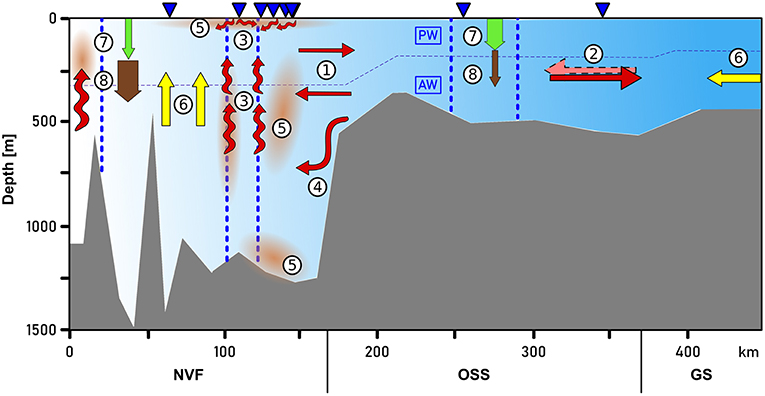
Figure 11. Conceptual figure of the different regimes in Scoresby Sund influencing the fjord carbon cycle. Two-dimensional circulation was observed at the entrance to Nordvestfjord with inflowing water below 400–500 m depth, and outflowing water above (1). Due to the width of the OSS, the formation of a three-dimensional circulation pattern consisting of outflowing water at the southern side and inflowing water at the northern side was possible (2). The import of meltwater (3) consists of rising meltwater plumes from submarine discharge and surface meltwater inflow. (4) indicates the deep overflow of Atlantic Water across the sill, filling the basin of Nordvestfjord. Currents, bottom topography, and meltwater discharge result in (5) plumes of high turbidity at the depth of surface and submarine meltwater discharge as well as resuspension. The distribution of nutrients is determined by upwelling caused by rising plumes of subglacial discharge, and by the import with Atlantic and Polar Water from the shelf (6). Arrows of (7) export production and (8) POC flux are scaled to the according magnitude. PW, Polar Water; AW, Atlantic Water.

Author Contributions

UJ and BK planned the expedition MSM56. MS, MH, and MI designed the study. MS, CB, AF, JG, UJ, BK, CK, and HvdJ acquired the data. AF and OZ provided hydrographic and light field data. HvdJ and CK corrected the flux data, and CB and JG the nutrient data. TK and CE planned and participated in the cruise MSM76, and analyzed the LADCP data. MS, MH, and MI interpreted the data, with help from co-authors. MS wrote the manuscript with contributions from all co-authors.

Funding

The Deutsche Forschungsgemeinschaft (DFG) and the Senatskommission für Ozeanographie were supporting the cruise MSM56 (MerMet 14-15 Koch). MS, MI, CK, and HvdJ were supported by the HGF Young Investigator Group SeaPump Seasonal and regional food web interactions with the biological pump, grant number VH-NG-1000. MS was additionally supported under HGF Young Investigator Group MarESys Marine Carbon and Ecosystem Feedbacks in the Earth System, grant number VH-NG-1301. The analysis regarding the circulation in Scoresby Sund (TK, CE) represents a contribution to the project OGreen79 (grant KA 3204/5-1) funded by the Deutsche Forschungsgemeinschaft (DFG) as part of the Special Priority Program (SPP)-1889 Regional Sea Level Change and Society. CE was supported by NSF Grant 1604076. DFKI acknowledges financial support by the MWK through Niedersachsen Vorab (ZN3480).

Conflict of Interest Statement

The authors declare that the research was conducted in the absence of any commercial or financial relationships that could be construed as a potential conflict of interest.

Acknowledgments

We thank the captain, crew, and the participants of RV Maria S. Merian for their assistance during the cruise MSM56. We would also like to thank the captain and the crew of RV Maria S. Merian for their professional and engaged work during expedition MSM76. Special thanks to Wilken-Jon von Appen for contributing with valuable ideas for the interpretation of physical oceanographic data, and Christiane Lorenzen and Laura Wischnewski for the biogeochemical measurements. We also acknowledge the help of Antonie Haas, Anne-Cathrin Wölfl, and Laura Hehemann for analyzing the fjord's bathymetry. We thank three reviewers for constructive and valuable comments that significantly helped us to improve the manuscript. Parts of this article have been subject of the Master thesis of MS (Seifert, 2018), which can be accessed online (https:\\epic.awi.de\47232\1\Miriam_Seifert_Master_Thesis.pdf).

References

Alldredge, A. L., and Crocker, K. M. (1995). Why do sinking mucilage aggregates accumulate in the water column? Sci. Total Environ. 165, 15–22. doi: 10.1016/0048-9697(95)04539-d

CrossRef Full Text | Google Scholar

Anderson, L. G., Jones, E. P., and Swift, J. H. (2003). Export production in the central Arctic Ocean evaluated from phosphate deficits. J. Geophys. Res. 108:3199. doi: 10.1029/2001JC001057

CrossRef Full Text | Google Scholar

Anderson, S. P., Drever, J. I., Frost, C. D., and Holden, P. (2000). Chemical weathering in the foreland of a retreating glacier. Geochim. Cosmochim. Acta 64, 1173–1189. doi: 10.1016/S0016-7037(99)00358-0

CrossRef Full Text | Google Scholar

Arendt, K. E., Agersted, M. D., Sejr, M. K., and Juul-Pedersen, T. (2016). Glacial meltwater influences on plankton community structure and the importance of top-down control (of primary production) in a NE Greenland fjord. Estuar. Coast. Shelf Sci. 183, 123–135. doi: 10.1016/j.ecss.2016.08.026

CrossRef Full Text | Google Scholar

Arendt, K. E., Nielsen, T. G., Rysgaard, S., and Tönnesson, K. (2010). Differences in plankton community structure along the Godthåbsfjord, from the Greenland Ice Sheet to offshore waters. Mar. Ecol. Progress Ser. 401, 49–62. doi: 10.3354/meps08368

CrossRef Full Text | Google Scholar

Armstrong, R. A., Lee, C., Hedges, J. I., Honjo, S., and Wakeham, S. G. (2001). A new, mechanistic model for organic carbon fluxes in the ocean based on the quantitative association of POC with ballast minerals. Deep Sea Res. Part II 49, 219–236. doi: 10.1016/s0967-0645(01)00101-1

CrossRef Full Text | Google Scholar

Arrigo, K. R., and van Dijken, G. L. (2015). Continued increases in Arctic Ocean primary production. Progress. Oceanogr. 136, 60–70. doi: 10.1016/j.pocean.2015.05.002

CrossRef Full Text | Google Scholar

Bates, N. R., Best, M. H. P., and Hansell, D. A. (2005). Spatio-temporal distribution of dissolved inorganic carbon and net community production in the Chukchi and Beaufort Seas. Deep Sea Res. Part II 52, 3303 – 3323. doi: 10.1016/j.dsr2.2005.10.005

CrossRef Full Text | Google Scholar

Beaird, N. L., Straneo, F., and Jenkins, W. (2018). Export of strongly diluted Greenland meltwater from a major glacial fjord. Geophys. Res. Lett. 45, 4163–4170. doi: 10.1029/2018gl077000

CrossRef Full Text | Google Scholar

Belcher, A., Iversen, M., Manno, C., Henson, S. A., Tarling, G. A., and Sanders, R. (2016). The role of particle associated microbes in remineralization of fecal pellets in the upper mesopelagic of the Scotia Sea, Antarctica. Limnol. Oceanogr. 61, 1049–1064. doi: 10.1002/lno.10269

CrossRef Full Text | Google Scholar

Bendtsen, J., Gustafsson, K. E., Rygaard, S., and Vang, T. (2007). “Physical conditions, dynamics and model simulations during the ice-free period of the Young Sound/Tyrolerfjord system,” in Carbon Cycling in Arctic Marine ecosystems: Case Study Young Sound, Meddr. Grønland, Bioscience, 58, eds. S. Rysgaard and R. N. Glud, 46–59.

Google Scholar

Bendtsen, J., Mortensen, J., and Rysgaard, S. (2015). Modelling subglacial discharge and its influence on ocean heat transport in Arctic fjords. Ocean Dynam. 65, 1535–1546. doi: 10.1007/s10236-015-0883-1

CrossRef Full Text | Google Scholar

Bhatia, M. P., Kujawinski, E. B., Das, S. B., Breier, C. F., Henderson, P. B., and Charette, M. A. (2013). Greenland meltwater as a significant and potentially bioavailable source of iron to the ocean. Nat. Geosci. 6, 274–278. doi: 10.1038/ngeo1746

CrossRef Full Text | Google Scholar

Boone, W., Rysgaard, S., Carlson, D. F., Meire, L., Kirillov, S., Mortensen, J., et al. (2018). Coastal freshening prevents fjord bottom water renewal in Northeast Greenland: a mooring study from 2003 to 2015. Geophys. Res. Lett. 45, 2726–2733. doi: 10.1002/2017gl076591

CrossRef Full Text | Google Scholar

Brown, G. H. (2002). Glacier meltwater hydrochemistry. Appl. Geochem. 17, 855–883. doi: 10.1016/s0883-2927(01)00123-8

CrossRef Full Text | Google Scholar

Burgers, T. M., Miller, L. A., Thomas, H., Else, B. G. T., Gosselin, M., and Papakyriakou, T. (2017). Surface water pCO₂ variations and sea-air CO₂ fluxes during summer in the Eastern Canadian Arctic. J. Geophys. Res. Oceans 122, 9663–9678. doi: 10.1002/2017JC013250

CrossRef Full Text | Google Scholar

Carr, J. R., Stokes, C. R., and Vieli, A. (2017). Threefold increase in marine-terminating outlet glacier retreat rates across the Atlantic Arctic: 1992–2010. Ann. Glaciol. 58, 72–91. doi: 10.1017/aog.2017.3

CrossRef Full Text | Google Scholar

Carroll, D., Sutherland, D. A., Hudson, B., Moon, T., Catania, G., Shroyer, E. L., et al. (2016). The impact of glacier geometry on meltwater plume structure and submarine melt in Greenland fjords. Geophys. Res. Lett. 43, 9739–9748. doi: 10.1002/2016GL070170

CrossRef Full Text | Google Scholar

Carroll, D., Sutherland, D. A., Shroyer, E. L., Nash, J. D., Catania, G. A., and Stearns, L. A. (2015). Modeling turbulent subglacial meltwater plumes: implications for fjord-scale buoyancy-driven circulation. Am. Meteorol. Soc. 45, 2169–2185. doi: 10.1175/JPO-D-15-0033.1

CrossRef Full Text | Google Scholar

Chu, V. W. (2014). Greenland ice sheet hydrology: a review. Progress Phys. Geogr. 38, 19–54. doi: 10.1177/0309133313507075

CrossRef Full Text | Google Scholar

Cowton, T., Sole, A., Nienow, P., Slater, D., Wilton, D., and Hanna, E. (2016). Controls on the transport of oceanic heat to Kangerdlugssuaq Glacier, East Greenland. J. Glaciol. 62, 1167–1180. doi: 10.1017/jog.2016.117

CrossRef Full Text | Google Scholar

Cross, J. N., Mathis, J. T., Bates, N. R., and Byrne, R. H. (2013). Conservative and non-conservative variations of total alkalinity on the southeastern Bering Sea shelf. Mar. Chem. 154, 100–112. doi: 10.1016/j.marchem.2013.05.012

CrossRef Full Text | Google Scholar

Death, R., Wadham, J. L., Monteiro, F., Le Brocq, A. M., Tranter, M., Ridgwell, A., et al. (2014). Antarctic ice sheet fertilises the Southern Ocean. Biogeosciences 11, 2635–2644. doi: 10.5194/bg-11-2635-2014

CrossRef Full Text | Google Scholar

Dickson, A. G., Sabine, C. L., and Christian , J. R. (Eds.). (2007). Guide to Best Practices for Ocean CO₂ Measurements. PICES Special Publication 3, IOCCP Report 8. Sidney, BC: North Pacific Marine Science Organization.

Google Scholar

Dowdeswell, J. A., Batchelor, C. L., Hogan, K. A., and Schenke, H.-W. (2016). “Nordvestfjord: a major East Greenland fjord system,” in Atlas of Submarine Glacial Landforms: Modern, Quaternary and Ancient, Memoirs, Vol. 46, eds. J. A. Dowdeswell, M. Canals, M. Jakobsson, B. J. Todd, E. K. Dowdeswell, and K. A. Hogan (London: Geological Society), 43–44. doi: 10.1144/m46.40

CrossRef Full Text | Google Scholar

Dowdeswell, J. A., Villinger, H., Whittington, R. J., and Marienfeld, P. (1993). Iceberg scouring in scoresby sund and on the East Greenland continental shelf. Mar. Geol. 111, 37–53. doi: 10.1016/0025-3227(93)90187-z

CrossRef Full Text | Google Scholar

Duprat, L. P. A. M., Bigg, G. R., and Wilton, D. J. (2016). Enhanced Southern Ocean marine productivity due to fertilization by giant icebergs. Nat. Geosci. 9, 219–221. doi: 10.1038/NGEO2633

CrossRef Full Text | Google Scholar

Enderlin, E. M., Carrigan, C. J., Kochtitzky, W. H., Cuadros, A., Moon, T., and Hamilton, G. S. (2018). Greenland iceberg melt variability from high-resolution satellite observations. Cryosphere 12, 565–575. doi: 10.5194/tc-12-565-2018

CrossRef Full Text | Google Scholar

Enderlin, E. M., and Howat, I. M. (2013). Submarine melt rate estimates for floating termini of Greenland outlet glaciers (2000–2010). J. Glaciol. 59, 67–75. doi: 10.3189/2013jog12j049

CrossRef Full Text | Google Scholar

Fransson, A., Chierici, M., Miller, L. A., Carnat, G., Shadwick, E., Thomas, H., et al. (2013). Impact of sea-ice processes on the carbonate system and ocean acidification at the ice-water interface of the Amundsen Gulf, Arctic Ocean. J. Geophys. Res. Oceans 118, 7001–7023. doi: 10.1002/2013jc009164

CrossRef Full Text | Google Scholar

Fried, M. J., Catania, G. A., Bartholomaus, T. C., Duncan, D., Davis, M., Stearns, L. A., et al. (2015). Distributed subglacial discharge drives significant submarine melt at a Greenland tidewater glacier. Geophys. Res. Lett. 42, 9328–9336. doi: 10.1002/2015GL065806

CrossRef Full Text | Google Scholar

Friedrichs, A., Schwalfenberg, K., Koch, B. P., and Zielinski, O. (2017). Physical Oceanography During MARIA S. MERIAN Cruise MSM56 (MECAF). Lower Saxony: Institute for Chemistry and Biology of the Marine Environment; Oldenburg: Carl-von-Ossietzky University of Oldenburg. doi: 10.1594/PANGAEA.871015

CrossRef Full Text

Friis, K., Körtzinger, A., and Wallace, D. W. R. (2003). The salinity normalization of marine inorganic carbon chemistry data. Geophys. Res. Lett. 30:1085. doi: 10.1029/2002GL015898

CrossRef Full Text | Google Scholar

Funder, S. (1972). Deglaciation of the Scoresby Sund fjord region, north-east Greenland. Fr. Bagges Kgl. Hofbogtrykkeri 4, 33–42

Google Scholar

Gade, H. G. (1979). Melting of ice in sea water: a primitive model with application to the Antarctic ice shelf and icebergs. J. Phys. Oceanogr. 9, 189–198.

Google Scholar

Glud, R. N., Rysgaard, S., Kühl, M., and Hansen, J. W. (2007). “The sea ice in Young Sound: implications for carbon cycling,” in Carbon Cycling in Arctic marine ecosystems: Case Study Young Sound, Meddr. Grønland, Bioscience, 58, eds. S. Rysgaard and R. N. Glud, 62–85.

Google Scholar

Gran, G. (1952). Determination of the equivalence point in potentiometric titrations. Part II. Analyst 77, 661–671. doi: 10.1039/an9527700661

CrossRef Full Text | Google Scholar

Guidi, L., Legendre, L., Reygondeau, G., Uitz, J., Stemmann, L., and Henson, S. A. (2015). A new look at ocean carbon remineralization for estimating deepwater sequestration. Glob. Biogeochem. Cycles 29, 1044–1059. doi: 10.1002/2014gb005063

CrossRef Full Text | Google Scholar

Hamm, C. E. (2002). Interactive aggregation and sedimentation of diatoms and clay-sized lithogenic material. Limnol. Oceanogr. 47, 1790–1795. doi: 10.4319/lo.2002.47.6.1790

CrossRef Full Text | Google Scholar

Hansell, D. A., and Carlson, C. A. (1998). Net community production of dissolved organic carbon. Glob. Biogeochem. Cycles 12, 443–453. doi: 10.1029/98gb01928

CrossRef Full Text | Google Scholar

Harada, N. (2016). Potential catastrophic reduction of sea ice in the western Arctic Ocean: Its impact on biogeochemical cycles and marine ecosystems. Glob. Planet. Change 136, 1–17. doi: 10.1016/j.gloplacha.2015.11.005

CrossRef Full Text | Google Scholar

Hawkings, J., Wadham, J., Tranter, M., Telling, J., Bagshaw, E., Beaton, A., et al. (2016). The Greenland Ice Sheet as a hot spot of phosphorus weathering and export in the Arctic. Glob. Biogeochem. Cycles 30, 191–210. doi: 10.1002/2015gb005237

CrossRef Full Text | Google Scholar

Hawkings, J. R., Wadham, J. L., Benning, L. G., Hendry, K. R., Tranter, M., Tedstone, A., et al. (2017). Ice sheets as a missing source of silica to the polar oceans. Nat. Commun. 8:14198. doi: 10.1038/ncomms14198

PubMed Abstract | CrossRef Full Text | Google Scholar

Hawkings, J. R., Wadham, J. L., Tranter, M., Lawson, E., Sole, A., Cowton, T., et al. (2015). The effect of warming climate on nutrient and solute export from the Greenland Ice Sheet. Geochem. Perspect. Lett. 1, 94–104. doi: 10.7185/geochemlet.1510

CrossRef Full Text | Google Scholar

Holinde, L., and Zielinski, O. (2016). Bio-optical characterization and light availability parameterization in Uummannaq Fjord and Vaigat-Disko Bay (West Greenland). Ocean Sci. 12, 117–128. doi: 10.5194/os-12-117-2016

CrossRef Full Text | Google Scholar

Hoppema, M., Goeyens, L., and Fahrbach, E. (2000). Intense nutrient removal in the remote area off Larsen Ice Shelf (Weddell Sea). Polar Biol. 23, 85–94. doi: 10.1007/s003000050012

CrossRef Full Text | Google Scholar

Hoppema, M., Middag, R., de Baar, H. J. W., Fahrbach, E., van Weerlee, E. M., and Thomas, H. (2007). Whole season net community production in the Weddell Sea. Polar Biol. 31, 101–111. doi: 10.1007/s00300-007-0336-5

CrossRef Full Text | Google Scholar

Hopwood, M. J., Carroll, D., Browning, T., Meire, L., Mortensen, J., Krisch, S., et al. (2018). Non-linear response of summertime marine productivity to increased meltwater discharge around Greenland. Nat. Commun. 9:3256. doi: 10.1038/s41467-018-05488-8

PubMed Abstract | CrossRef Full Text | Google Scholar

Hopwood, M. J., Connelly, D. P., Arendt, K. E., Juul-Pedersen, T., Stinchcombe, M. C., Meire, L., et al. (2016). Seasonal changes in Fe along a glaciated Greenlandic fjord. Front. Earth Sci. 4:15. doi: 10.3389/feart.2016.00015

CrossRef Full Text | Google Scholar

Iversen, M. H., Nowald, N., Ploug, H., Jackson, G. A., and Fischer, G. (2010). High resolution profiles of vertical particulate organic matter export off Cape Blanc, Mauritania: degradation processes and ballasting effects. Deep Sea Res. Part I 57, 771–784. doi: 10.1016/j.dsr.2010.03.007

CrossRef Full Text | Google Scholar

Iversen, M. H., and Ploug, H. (2010). Ballast minerals and the sinking carbon flux in the ocean: carbon-specific respiration rates and sinking velocity of marine snow aggregates. Biogeosciences 7, 2613–2624. doi: 10.5194/bg-7-2613-2010

CrossRef Full Text | Google Scholar

Iversen, M. H., and Robert, M. L. (2015). Ballasting effects of smectite on aggregate formation and export from a natural plankton community. Mar. Chem. 175, 18–27. doi: 10.1016/j.marchem.2015.04.009

CrossRef Full Text | Google Scholar

Jennings, J. C. Jr, Gordon, L. I., and Nelson, D. M. (1984). Nutrient depletion indicates high primary productivity in the Weddell Sea. Nature 309, 52–54.

Google Scholar

Johnson, K. M., Wills, K. D., Butler, D. B., Johnson, W. K., and Wong, C. S. (1993). Coulometric total carbon dioxide analysis for marine studies: maximizing the performance of an automated gas extraction system and coulometric detector. Mar. Chem. 44, 167–187. doi: 10.1016/0304-4203(93)90201-x

CrossRef Full Text | Google Scholar

Jones, E. M., Bakker, D. C. E., Venables, H. J., Whitehouse, M. J., Korb, R. E., and Watson, A. J. (2010). Rapid changes in surface water carbonate chemistry during Antarctic sea ice melt. Tellus B 62, 621–635. doi: 10.3402/tellusb.v62i5.16611

CrossRef Full Text | Google Scholar

Juul-Pedersen, T., Arendt, K. E., Mortensen, J., Blicher, M. E., Søgaard, D. H., and Rysgaard, S. (2015). Seasonal and interannual phytoplankton production in a sub-Arctic tidewater outlet glacier fjord, SW Greenland. Mar. Ecol. Progress Ser. 524, 27–38. doi: 10.3354/meps11174

CrossRef Full Text | Google Scholar

Kanna, N., Sugiyama, S., Ohashi, Y., Sakakibara, D., Fukamachi, Y., and Nomura, D. (2018). Upwelling of macronutrients and dissolved inorganic carbon by a subglacial freshwater driven plume in Bowdoin Fjord, northwestern Greenland. J. Geophys. Res. Biogeosci. 123, 1666–1682. doi: 10.1029/2017jg004248

CrossRef Full Text | Google Scholar

Kattner, G., and Becker, H. (1991). Nutrients and organic nitrogenous compounds in the marginal ice zone of the Fram Strait. J. Mar. Syst. 2, 385–394. doi: 10.1016/0924-7963(91)90043-t

CrossRef Full Text | Google Scholar

Khan, S. A., Kjær, K. H., Bevis, M., Bamber, J. L., Wahr, J., Kjeldsen, K. K., et al. (2014). Sustained mass loss of the northeast Greenland ice sheet triggered by regional warming. Nat. Clim. Change 4, 292–299. doi: 10.1038/nclimate2161

CrossRef Full Text | Google Scholar

Koch, B. P. (2016). Short Cruise Report Maria S. Merian MSM56. Available online at: https://www.ldf.uni-hamburg.de/merian/wochenberichte/wochenberichte-merian/msm55-msm57/msm56-scr.pdf (accessed October 2, 2018).

Koziorowska, K., Kuliński, K., and Pempkowiak, J. (2016). Sedimentary organic matter in two Spitsbergen fjords: terrestrial and marine contributions based on carbon and nitrogen contents and stable isotopes composition. Continen. Shelf Res. 113, 38–46. doi: 10.1016/j.csr.2015.11.010

CrossRef Full Text | Google Scholar

Lee, K. (2001). Global net community production estimated from the annual cycle of surface water total dissolved inorganic carbon. Limnol. Oceanogr. 46, 1287–1297. doi: 10.4319/lo.2001.46.6.1287

CrossRef Full Text | Google Scholar

Lewis, S. M., and Smith, L. C. (2009). Hydrologic drainage of the Greenland Ice Sheet. Hydrol. Process. 23, 2004–2011. doi: 10.1002/hyp.7343

CrossRef Full Text | Google Scholar

Lund-Hansen, L. C., Andersen, T. J., Nielsen, M. H., and Pejrup, M. (2010). Suspended matter, Chl-a, CDOM, grain sizes, and optical properties in the Arctic fjord-type estuary, Kangerlussuaq, West Greenland during summer. Estuar. Coasts 33, 1442–1451. doi: 10.1007/s12237-010-9300-7

CrossRef Full Text | Google Scholar

Lund-Hansen, L. C., Hawes, I., Holtegaard Nielsen, M., Dahllöf, I., and Sorrell, B. K. (2018). Summer meltwater and spring sea ice primary production, light climate and nutrients in an Arctic estuary, Kangerlussuaq, west Greenland. Arct. Antarct. Alpine Res. 50:S100025. doi: 10.1080/15230430.2017.1414468

CrossRef Full Text | Google Scholar

Martin, J. H., Knauer, G. A., Karl, D. M., and Broenkow, W. W. (1987). VERTEX: carbon cycling in the northeast Pacific. Deep Sea Res. 34, 267–285. doi: 10.1016/0198-0149(87)90086-0

CrossRef Full Text | Google Scholar

Mathis, J. T., Bates, N. R., Hansell, D. A., and Babila, T. (2009). Net community production in the northeastern Chukchi Sea. Deep Sea Res. Part II 56, 1213–1222. doi: 10.1016/j.dsr2.2008.10.017

CrossRef Full Text | Google Scholar

Meire, L., Meire, P., Struyf, E., Krawczyk, D. W., Arendt, K. E., Yde, J. C., et al. (2016a). High export of dissolved silica from the Greenland Ice Sheet. Geophys. Res. Lett. 43, 9173–9182. doi: 10.1002/2016gl070191

CrossRef Full Text | Google Scholar

Meire, L., Mortensen, J., Meire, P., Juul-Pedersen, T., Sejr, M. K., Rysgaard, S., et al. (2017). Marine-terminating glaciers sustain high productivity in Greenland fjords. Glob. Change Biol. 23, 5344–5357. doi: 10.1111/gcb.13801

PubMed Abstract | CrossRef Full Text | Google Scholar

Meire, L., Mortensen, J., Rysgaard, S., Bendtsen, J., Boone, W., Meire, P., and Meysman, F. J. R. (2016b). Spring bloom dynamics in a subarctic fjord influenced by tidewater outlet glaciers (Godthaabsfjord, SW Greenland). J. Geophys. Res. Biogeosci. 121, 1581–1592. doi: 10.1002/2015JG003240

CrossRef Full Text | Google Scholar

Meire, L., Søgaard, D. H., Mortensen, J., Meysman, F. J. R., Soetaert, K., Arendt, K. E., et al. (2015). Glacial meltwater and primary production are drivers of strong CO₂ uptake in fjord and coastal waters adjacent to the Greenland Ice Sheet. Biogeosciences 12, 2347–2363. doi: 10.5194/bg-12-2347-2015

CrossRef Full Text | Google Scholar

Middelbo, A. B., Sejr, M. K., Arendt, K. E., and Møller, E. F. (2018). Impact of glacial meltwater on spatiotemporal distribution of copepods and their grazing impact in Young Sound NE, Greenland. Limnol. Oceanogr. 63, 322–336. doi: 10.1002/lno.10633

CrossRef Full Text | Google Scholar

Millan, R., Rignot, E., Mouginot, J., Wood, M., Bjørk, A. A., and Morlighem, M. (2018). Vulnerability of southeast Greenland glaciers to warm Atlantic Water from Operation IceBridge and Ocean Melting Greenland data. Geophys. Res. Lett. 45, 2688–2696. doi: 10.1002/2017gl076561

PubMed Abstract | CrossRef Full Text | Google Scholar

Moon, T., Sutherland, D. A., Carroll, D., Felikson, D., Kehrl, L., and Straneo, F. (2017). Subsurface iceberg melt key to Greenland fjord freshwater budget. Nat. Geosci. 11, 49–54. doi: 10.1038/s41561-017-0018-z

CrossRef Full Text | Google Scholar

Mortensen, J., Bendtsen, J., Motyka, R. J., Lennert, K., Truffer, M., Fahnestock, M., and Rysgaard, S. (2013). On the seasonal freshwater stratification in the proximity of fast-flowing tidewater outlet glaciers in a sub-Arctic sill fjord. J. Geophys. Res. Oceans 118, 1382–1395. doi: 10.1002/jgrc.20134

CrossRef Full Text | Google Scholar

Munro, D. R., Lovenduski, N. S., Stephens, B. B., Newberger, T., Arrigo, K. R., Takahashi, T., et al. (2015). Estimates of net community production in the Southern Ocean determined from time series observations (2002–2011) of nutrients, dissolved inorganic carbon, and surface ocean pCO₂ in Drake Passage. Deep Sea Research Part II 114, 49–63. doi: 10.1016/j.dsr2.2014.12.014

CrossRef Full Text | Google Scholar

Murray, C., Markager, S., Stedmon, C. A., Juul-Pedersen, T., Sejr, M. K., and Bruhn, A. (2015). The influence of glacial melt water on bio-optical properties in two contrasting Greenlandic fjords. Estuar. Coast. Shelf Sci. 163, 72–83. doi: 10.1016/j.ecss.2015.05.041

CrossRef Full Text | Google Scholar

Nienow, P. W., Sole, A. J., Slater, D. A., and Cowton, T. R. (2017). Recent advances in our understanding of the role of meltwater in the Greenland Ice Sheet system. Curr. Clim. Change Rep. 3, 330–344. doi: 10.1007/s40641-017-0083-9

CrossRef Full Text | Google Scholar

Nurser, A. J. G., and Bacon, S. (2014). The rossby radius in the Arctic Ocean. Ocean Sci. 10, 967–975. doi: 10.5194/os-10-967-2014

CrossRef Full Text | Google Scholar

Ó Cofaigh, C., Dowdeswell, J. A., and Grobe, H. (2001). Holocene glacimarine sedimentation, inner Scoresby Sund, East Greenland: the influence of fast-flowing ice-sheet outlet glaciers. Mar. Geol. 175, 103–129. doi: 10.1016/s0025-3227(01)00117-7

CrossRef Full Text | Google Scholar

Padman, L., and Erofeeva, S. (2004). A barotropic inverse tidal model for the Arctic Ocean. Geophys. Res. Lett. 31:L02303. doi: 10.1029/2003GL019003

CrossRef Full Text | Google Scholar

Pilcher, D. J., Siedlecki, S. A., Hermann, A. J., Coyle, K. O., Mathis, J. T., and Evans, W. (2018). Simulated impact of glacial runoff on CO₂ uptake in the Gulf of Alaska. Geophys. Res. Lett. 45, 880–890. doi: 10.1002/2017gl075910

CrossRef Full Text | Google Scholar

Ploug, H., Iversen, M. H., Koski, M., and Buitenhuis, E. T. (2008). Production, oxygen respiration rates, and sinking velocity of copepod fecal pellets: Direct measurements of ballasting by opal and calcite. Limnol. Oceanogr. 53, 469–476. doi: 10.4319/lo.2008.53.2.0469

CrossRef Full Text | Google Scholar

Redfield, A. C., Ketchum, B. H., and Richards, F. A. (1963). “The influence of organisms on the composition of sea-water,” in The Composition of Seawater: Comparative and Descriptive Oceanography. The Sea: Ideas and Observations on Progress in the Study of the Seas, vol. 2, ed. M. N. Hill (New York, NY: Wiley-Interscience, 26–77

Reisdorph, S. C., and Mathis, J. T. (2014). The dynamic controls on carbonate mineral saturation states and ocean acidification in a glacially dominated estuary. Estuar. Coast. Shelf Sci. 144, 8–18. doi: 10.1016/j.ecss.2014.03.018

CrossRef Full Text | Google Scholar

Reisdorph, S. C., and Mathis, J. T. (2015). Assessing net community production in a glaciated Alaskan fjord. Biogeosciences 12, 5185–5198. doi: 10.5194/bg-12-5185-2015

CrossRef Full Text | Google Scholar

Richlen, M. L., Zielinski, O., Holinde, L., Tillmann, U., Cembella, A., Lyu, Y., and Anderson, D. M. (2016). Distribution of Alexandrium fundyense (Dinophyceae) cysts in Greenland and Iceland, with an emphasis on viability and growth in the Arctic. Mar. Ecol. Progress Ser. 547, 33–46. doi: 10.3354/meps11660

PubMed Abstract | CrossRef Full Text | Google Scholar

Rignot, E., and Kanagaratnam, P. (2006). Changes in the velocity structure of the Greenland Ice Sheet. Science 311, 986–990. doi: 10.1126/science.1121381

PubMed Abstract | CrossRef Full Text | Google Scholar

Rudels, B., Anderson, L. G., and Jones, E. P. (1996). Formation and evolution of the surface mixed layer and halocline of the Arctic Ocean. J. Geophys. Res. 101, 8807–8821. doi: 10.1029/96jc00143

CrossRef Full Text | Google Scholar

Rudels, B., Fahrbach, E., Meincke, J., Budéus, G., and Eriksson, P. (2002). The east greenland current and its contribution to the Denmark Strait overflow. ICES J. Mar. Sci. 59, 1133–1154. doi: 10.1006/jmsc.2002.1284

CrossRef Full Text | Google Scholar

Rysgaard, S., Bendtsen, J., Pedersen, L. T., Ramløv, H., and Glud, R. N. (2009). Increased CO₂ uptake due to sea ice growth and decay in the Nordic Seas. J. Geophys. Res. 114:C09011. doi: 10.1029/2008JC005088

CrossRef Full Text | Google Scholar

Rysgaard, S., and Glud, R. N. (2007). “Carbon cycling and climate change: predictions for a high Arctic marine ecosystem (Young Sound, NE Greenland),” in Carbon Cycling in Arctic Marine Ecosystems: Case Study Young Sound, Meddr. Grønland, Bioscience, 58, eds. S. Rysgaard and R. N. Glud, 206–214.

Google Scholar

Rysgaard, S., Mortensen, J., Juul-Pedersen, T., Sørensen, L. L., Lennert, K., Søgaard, D. H., et al. (2012). High air–sea CO₂ uptake rates in nearshore and shelf areas of Southern Greenland: temporal and spatial variability. Mar. Chem. 128-129, 26–33. doi: 10.1016/j.marchem.2011.11.002

CrossRef Full Text | Google Scholar

Rysgaard, S., and Nielsen, T. G. (2006). Carbon cycling in a high-arctic marine ecosystem – Young Sound, NE Greenland. Progress Oceanogr. 71, 426–445. doi: 10.1016/j.pocean.2006.09.004

CrossRef Full Text | Google Scholar

Rysgaard, S., and Sejr, M. K. (2007). “Vertical flux of particluate organic matter in a High Arctic Fjord: Relative importance of terrestrial and marine sources,” in Carbon Cycling in Arctic Marine ecosystems: Case Study Young Sound, Meddr. Grønland, Bioscience, 58, eds. S. Rysgaard and R. N. Glud, 110–119.

Google Scholar

Rysgaard, S., Vang, T., Stjernholm, M., Rasmussen, B., Windelin, A., and Kiilsholm, S. (2003). Physical conditions, carbon transport, and climate change impacts in a northeast Greenland fjord. Arct. Antarct. Alpine Res. 35, 301–312. doi: 10.1657/1523-0430(2003)035[0301:pcctac]2.0.co;2

CrossRef Full Text | Google Scholar

Ryu, J.-S., and Jacobson, A. D. (2012). CO₂ evasion from the Greenland Ice Sheet: a new carbon-climate feedback. Chem. Geol. 320-321, 80–95. doi: 10.1016/j.chemgeo.2012.05.024

CrossRef Full Text | Google Scholar

Schlitzer, R. (2004) version 4.7.10. Ocean data view. Available online at: https://odv.awi.de/ (accessed July 16, 2017).

Sciascia, R., Straneo, F., Cenedese, C., and Heimbach, P. (2013). Seasonal variability of submarine melt rate and circulation in a East Greenland fjord. J. Geophys. Res. Oceans 118, 2492–2506. doi: 10.1002/jgrc.20142

CrossRef Full Text | Google Scholar

Seifert, M. (2018). Carbon Cycling in an Arctic Fjord (Scoresby Sund, East Greenland) With Regard to the Influence of Glacial Meltwater Discharge. Bremen: Master's thesis, Universität Bremen. hdl:10013/epic.6d5579b0-8959-4316-a8e8-53accc603996

Google Scholar

Sejr, M. K., Krause-Jensen, D., Rysgaard, S., Sørensen, L. L., Christensen, P. B., and Glud, R. N. (2011). Air-sea flux of CO₂ in arctic coastal waters influenced by glacial melt water and sea ice. Tellus B 63, 815–822. doi: 10.1111/j.1600-0889.2011.00540.x

CrossRef Full Text | Google Scholar

Smith, R. W., Bianchi, T. S., Allison, M., Savage, C., and Galy, V. (2015). High rates of organic carbon burial in fjord sediments globally. Nat. Geosci. 8, 450–453. doi: 10.1038/ngeo2421

CrossRef Full Text | Google Scholar

Sørensen, H. L., Meire, L., Juul-Pedersen, T., de Stigter, H. C., Meysman, F. J. R., Rysgaard, S., et al. (2015). Seasonal carbon cycling in a Greenlandic fjord: an integrated pelagic and benthic study. Mar. Ecol. Progress Ser. 539, 1–17. doi: 10.3354/meps11503

CrossRef Full Text | Google Scholar

Straneo, F., and Cenedese, C. (2015). The dynamics of Greenland's glacial fjords and their role in climate. Ann. Rev. Mar. Sci. 7, 89–112. doi: 10.1146/annurev-marine-010213-135133

PubMed Abstract | CrossRef Full Text | Google Scholar

Straneo, F., Heimbach, P., Sergienko, O., Hamilton, G., Catania, G., Griffies, S., et al. (2013). Challenges to understanding the dynamic response of Greenland's marine terminating glaciers to oceanic and atmospheric forcing. Bull. Am. Meteorol. Soc. 94, 1131–1144. doi: 10.1175/BAMS-D-12-00100.1

CrossRef Full Text | Google Scholar

Straneo, F., Sutherland, D. A., Holland, D., Gladish, C., Hamilton, G. S., Johnson, H. L., et al. (2012). Characteristics of ocean waters reaching Greenland's glaciers. Ann. Glaciol. 53, 202–210. doi: 10.3189/2012AoG60A059

CrossRef Full Text | Google Scholar

Thamdrup, B., Glud, R. N., and Hansen, J. W. (2007). “Benthic carbon cycling in Young Sound, Northeast Greenland,” in Carbon Cycling in Arctic Marine Ecosystems: Case Study Young Sound, Meddr. Grønland, Bioscience, 58, eds. S. Rysgaard and R. N. Glud, 138–157.

Google Scholar

Turner, J. T. (2015). Zooplankton fecal pellets, marine snow, phytodetritus and the ocean's biological pump. Progress Oceanogr. 130, 205–248. doi: 10.1016/j.pocean.2014.08.005

CrossRef Full Text | Google Scholar

Ulfsbo, A., Cassar, N., Korhonen, M., van Heuven, S., Hoppema, M., Kattner, G., et al. (2014). Late summer net community production in the central Arctic Ocean using multiple approaches. Glob. Biogeochem. Cycles 28, 1129–1148. doi: 10.1002/2014gb004833

CrossRef Full Text | Google Scholar

van den Broeke, M. R., Enderlin, E. M., Howat, I. M., and Noël, B. P. Y. (2016). On the recent contribution of the Greenland ice sheet to sea level change. Cryosphere 10, 1933–1946. doi: 10.5194/tc-10-1933-2016

CrossRef Full Text | Google Scholar

van der Jagt, H., Friese, C., Stuut, J.-B. W., Fischer, G., and Iversen, M. H. (2018). The ballasting effect of Saharan dust deposition on aggregate dynamics and carbon export: aggregation, settling, and scavenging potential of marine snow. Limnol. Oceanogr. 63, 1386–1394. doi: 10.1002/lno.10779

CrossRef Full Text | Google Scholar

Wadham, J. L., Hawkings, J., Telling, J., Chandler, D., Alcock, J., O'Donnell, E., et al. (2016). Sources, cycling and export of nitrogen on the Greenland Ice Sheet. Biogeosciences 13, 6339–6352. doi: 10.5194/bg-13-6339-2016

CrossRef Full Text | Google Scholar

Walsh, K. M., Howat, I. M., Ahn, Y., and Enderlin, E. M. (2012). Changes in the marine-terminating glaciers of central east Greenland, 2000–2010. Cryosphere 6, 211–220. doi: 10.5194/tc-6-211-2012

CrossRef Full Text | Google Scholar

Wesławski, J. M., and Legeżyńska, J. (1998). Glaciers caused zooplankton mortality? J. Plankton Res. 20, 1233–1240

Google Scholar

Wiedmann, I., Reigstad, M., Marquardt, M., Vader, A., and Gabrielsen, T. M. (2016). Seasonality of vertical flux and sinking particle characteristics in an ice-free high arctic fjord – Different from subarctic fjords? J. Mar. Syst. 154, 192–205. doi: 10.1016/j.jmarsys.2015.10.003

CrossRef Full Text | Google Scholar

Williams, P. J. I. (1993). On the definition of plankton production terms. ICES Mar. Sci. Sympos. 197, 9–19

Zajaczkowski, M., Nygård, H., Hegseth, E. N., and Berge, J. (2010). Vertical flux of particulate matter in an Arctic fjord: the case of lack of the sea-ice cover in Adventfjorden 2006–2007. Polar Biol. 33, 223–239. doi: 10.1007/s00300-009-0699-x

CrossRef Full Text | Google Scholar

Zhu, Z.-Y., Wu, Y., Liu, S.-M., Wenger, F., Hu, J., Zhang, J., et al. (2016). Organic carbon flux and particulate organic matter composition in Arctic valley glaciers: examples from the Bayelva River and adjacent Kongsfjorden. Biogeosciences 13, 975–987. doi: 10.5194/bg-13-975-2016

CrossRef Full Text | Google Scholar