Targeted Sampling by Autonomous Underwater Vehicles

1. Introduction

Traditional ship-based methods for detecting and sampling dynamic ocean features are often laborious and difficult, and long-term tracking of such features using ships is practically impossible. Consequently, there is a growing effort toward enabling autonomous underwater vehicles (AUVs) to autonomously find, track, and sample ephemeral oceanographic features. Several studies (Cruz and Matos, 2010a,b; Petillo et al., 2010; Cazenave et al., 2011; Zhang et al., 2012a) have used AUVs to detect and track the thermocline based on temperature gradients in the vertical dimension. In Petillo and Schmidt (2014), two AUVs collaboratively surveyed internal waves by using adaptive thermocline tracking and vehicle-to-vehicle track-and-trail behaviors via acoustic communications. AUVs were also used to locate seafloor hydrothermal vents (German et al., 2008; Paduan et al., 2018), trace chemical plumes (Farrell et al., 2005; Kukulya et al., 2018), and survey oil plumes emanating from a damaged wellhead (Camilli et al., 2010; Zhang et al., 2011). The AUV detected the plume based on a proxy signal (e.g., optical backscatter signal for hydrothermal vent plumes) and followed a tracking strategy to trace the plume source and map the plume field. In addition to using a suite of physical, chemical, and bulk biological sensors, some AUVs are now equipped with water samplers to take advantage of the vehicle's mobility to collect material while underway (Camilli et al., 2010; Ryan et al., 2010a; Govindarajan et al., 2015; Pargett et al., 2015; Wulff et al., 2016; Billings et al., 2017; Scholin et al., 2017).

In parallel with AUV hardware developments, a long-sought goal is to develop onboard intelligence that allows the AUV to autonomously assess prevailing conditions and determine when and where to focus survey observations and water sample collections. We call this “targeted sampling”—the use of AUVs to detect specific oceanic features based on real-time analysis of sensor data, and to respond to detection through vehicle path adaptation and water sample acquisition. Different from pre-programmed missions, the AUV adapts behavior in real time to track, map, and sample the target. Scientific insights into particular ocean phenomena are used to derive AUV algorithms for executing targeted sampling while taking advantage of the vehicle's flexible behaviors and growing endurance. In section 2, we present methodology and results from four field experiments that are representative of these growing capabilities. We conclude and propose future work in section 3.

2. AUV Targeted Sampling Methods and Field Experiments

The design principle underlying targeted sampling methods is to combine oceanographic knowledge of ocean phenomena of interest, and AUV capabilities that enable effective observational studies of the targeted feature. This combination, implemented by onboard signal processing, permits studies of the targeted feature at temporal and spatial resolutions not previously possible. Example field experiments highlighted here represent the studies of two coastal ocean phenomena—harmful algal blooms (HABs) and frontal systems, and one open-ocean phenomenon—the deep chlorophyll maximum (DCM) layer.

2.1. Capturing Peak Samples in a Phytoplankton Patch

Phytoplankton distributions in the ocean are patchy, and this patchiness has consequences for many ecosystem processes including primary production, the survival and growth of zooplankton and fish larvae, and the development of HABs (Lasker, 1975; Cowles et al., 1998; McManus et al., 2008; Ryan et al., 2008, 2010c; Sullivan et al., 2010). A common manifestation of patchiness is the formation of a vertically limited layer of maximum plankton abundance within the water column. In coastal ecosystems these layers can have small vertical scales, with a thickness ranging from <1 m to a few meters (Cowles et al., 1998; McManus et al., 2008; Ryan et al., 2010c). To study the planktonic community in layers, it is critical to acquire water samples within the areas of high abundance and vertically within the layer as it fluctuates in space and time.

Traditionally, Niskin bottles are lowered from the ship deck to take water samples. Locating a phytoplankton layer requires a human operator to inspect the cast profiles of chlorophyll fluorescence and manually determine triggering depths. This process is difficult to sustain for extensive surveys of mesoscale (~100 km) features, and the 1-m vertical scale of the bottle makes it difficult to localize sample acquisition within phytoplankton layers having small (<1 m) vertical scales. To advance capabilities for high-resolution mapping and sampling of these features, we enabled an AUV to autonomously find the phytoplankton layer within vehicle profiles of high-resolution surveys and trigger water sampling precisely in the layer. Our Dorado AUV is equipped with 20 (previously 10) syringe-like water samplers, called “gulpers” (Ryan et al., 2010a, bottom photo in Figure 1). Once triggered, each gulper acquires a 1.5-l water sample in 1–2 s. A HOBI Labs HydroScat-2 sensor measures chlorophyll fluorescence at 700 nm wavelength and optical backscatter at 420 and 700 nm wavelengths. Consistency of gulper triggering within the phytoplankton layer is essential to successful sampling. We designed a peak-capture algorithm to meet this challenge.

FIGURE 1

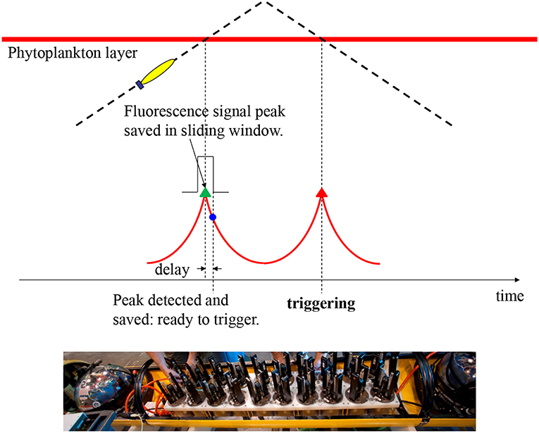
Figure 1. Illustration of the AUV algorithm for capturing peak samples in a phytoplankton patch. On the AUV's yo-yo trajectory through a phytoplankton layer, the vehicle detects the peak chlorophyll fluorescence (with delay) on the first crossing, and saves the peak signal level. On the second crossing, the AUV triggers sampling at the saved peak fluorescence level with no delay. The bottom photo (courtesy of Todd Walsh) shows 20 “gulper” samplers installed in the midsection of a Dorado-class AUV.

In any real-time gradient-based peak detection algorithm, a detection delay is unavoidable—the peak is detected only when it has just passed. Such a delay is especially problematic for a thin layer because a small delay will miss the peak. To overcome this peak-detection delay problem, our algorithm (Zhang et al., 2010) takes advantage of the AUV's yo-yo trajectory (in the vertical dimension), as illustrated in Figure 1. In one yo-yo cycle, e.g., an ascent profile followed by a descent profile, the vehicle crosses the layer twice, measuring a fluorescence peak at each crossing. At two consecutive crossings separated by a short distance (< several hundred meters), the two peaks are expected to have similar signal levels. On the vehicle's first crossing (on the ascent profile), peak detection (by tracking the fluorescence signal's slope) comes with a delay, but a sliding window saves the true peak value. On the second crossing (on the descent profile), water sampling is triggered the moment the fluorescence measurement reaches the saved peak value, resulting in sample capture right on the peak. If the second peak is slightly lower than the first (i.e., the saved signal peak level), no triggering will occur. This actually serves our objective of sampling only high peaks. Conversely, if the second peak is slightly higher than the first, sampling will be triggered at a signal level slightly before (hence slightly lower than) the second peak, yet already at a high near-peak level. The algorithm keeps track of the fluorescence background level and the baseline of the peaks in real time to ensure that peak detection is tuned to ambient conditions. The algorithm cross-checks for concurrent high values of optical backscatter to ensure that sampling targets true peaks of planktonic particles and not physiologically-controlled variations in fluorescence.

This peak-capture algorithm has been running on the Dorado AUV in a series of field programs since 2009. In the spring of 2015, Monterey Bay, CA experienced the most toxic HAB event ever recorded in this region (Ryan et al., 2017), caused by diatoms of the genus Pseudo-nitzschia. Two AUV missions (during upwelling relaxation and intensification, respectively) on a transect in the southern bay are shown in Figure 2. The AUV ran on a yo-yo trajectory between 2-m depth and the shallower of 75-m depth and 10-m altitude above the seabed. The depth of the HAB biomass maximum varied between near surface and 30-m depth. In this study, two 2nd-generation Environmental Sample Processors (2G-ESPs) (Scholin, 2013; Scholin et al., 2017) were moored at fixed depths of 4 and 6 m in the southern and northern bay, respectively. The ESP measurements provided key information for planning AUV deployments, but they missed HAB peaks when the local biomass was deeper than the sample intake of the moored ESPs. In contrast, the Dorado AUV mobility and the peak-capture algorithm enabled consistent sampling within the maximum HAB biomass, as shown in Figure 2B. Analyses of the gulper water samples showed very high concentrations of Pseudo-nitzschia (Figure 2A) and particulate domoic acid (pDA) (Figure 2B), the biotoxin within their cells.

FIGURE 2

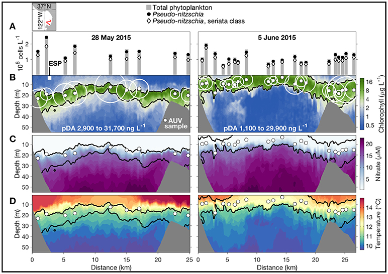
Figure 2. In May-June 2015, the Dorado AUV acquired water samples precisely from the HAB layer in two missions on a transect in the southern Monterey Bay, during upwelling relaxation (left) and intensification (right). The AUV transect's location is shown in the upper-left map. The AUV started from the southeast end of the transect. (A) Cell counts from microscopy, shown directly above the sample locations (indicated by the small solid white circles in B–D). (B–D) Chlorophyll concentration, nitrate concentration, and temperature along the AUV transect. In (B), the pDA concentration of each sample is represented by the size of the open white circle, and the range of pDA in each transect is noted. The position and depth of the moored 2G-ESP is indicated by the white square in (B). Adapted from Ryan et al. (2017) with permission.

Whether a patch is near the surface, in a subsurface layer, or near the seabed, the peak-capture algorithm is effective because it applies signal processing in the time domain throughout the full depth range of AUV profiles. For example, studies of larval ecology employing this algorithm in Monterey Bay in October 2009 detected the highest larval abundances in a dense phytoplankton patch that was subducted to the seabed within an upwelling front (Ryan et al., 2014). A ship-based survey would not have targeted near-seabed waters or provided the high-resolution data required to detect the patch within the small-scale front. In contrast, the AUV resolved the physical-biological interaction and precisely targeted the feature of interest.

2.2. Classifying and Sampling Distinct Water Types Across a Coastal Upwelling Front

Coastal upwelling is a wind-driven physical process that brings cooler, saltier, and usually nutrient-rich deep water upward to replace warmer, fresher, nutrient-depleted surface water. In addition to bringing up nutrients to support primary production, upwelling generates dynamic fronts that influence marine ecology in a variety of ways (Barber and Smith, 1981). Fronts occur frequently in the major eastern boundary upwelling systems of the northeastern and southeastern Atlantic and Pacific (Smith, 1981). In Monterey Bay, when a northwesterly wind persists along the coast, upwelling develops at Point Año Nuevo, and the cold upwelling filaments spread southeastward across the mouth of the bay, as shown in the satellite sea surface temperature (SST) images (Figure 3). In the northern bay, however, the water column typically remains stratified (warm at surface and cold at depth) because that region is sheltered from upwelling-inducing wind by the Santa Cruz mountains, and sheltered from the upwelling filaments by the coastal recess, thus forming an “upwelling shadow” (Graham et al., 1992; Graham and Largier, 1997). The boundary between the stratified, biologically enriched water of the upwelling shadow, and the unstratified, biologically impoverished water transported southeastward from the Point Año Nuevo upwelling center, is called the “upwelling front.” Upwelling fronts support enriched phytoplankton and zooplankton populations, as well as physical processes that can locally enhance plankton aggregation and nutrient supply (Woodson et al., 2009; Ryan et al., 2010b,c, 2014; Harvey et al., 2012), thus playing an important role in structuring ocean ecosystems. Detection and sampling of upwelling fronts is important for ecological studies of coastal upwelling systems (Zhang et al., 2015).

FIGURE 3

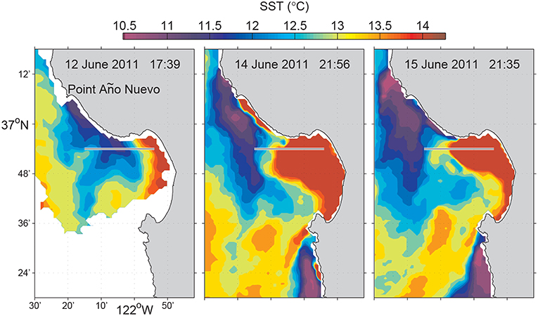
Figure 3. Satellite SST of Monterey Bay during the June 2011 experiment. The line along 36.9°N (from 121.9°W to 122.25°W) marks the Dorado AUV's 31-km transect. Reused from Zhang et al. (2012c) with permission. Time is in Pacific Daylight Time (PDT).

Upwelling fronts move due to variations in wind and ocean circulation, as shown in Figure 3. These fronts are also associated with strong physical and biological gradients that occur on small spatial scales. These attributes of fronts present challenges to effective observation and sampling. Traditional ship-based methods are incapable of autonomously detecting and sampling fronts. Further, they are laborious and costly¹. The physical process of upwelling offers an excellent classifier for distinguishing upwelling from stratified water columns: the former is much more homogeneous vertically than the latter. An AUV yo-yo trajectory provides a convenient way to measure water column vertical homogeneity. Hence we developed an AUV algorithm to autonomously distinguish between upwelling and stratified water columns based on vertical temperature homogeneity, and to accurately locate an upwelling front based on the horizontal gradient of vertical temperature homogeneity (Zhang et al., 2012b,c). We defined a metric, the vertical temperature homogeneity index (VTHI), as follows (Zhang et al., 2012c):

$\begin{array}{ll}VTHI=\frac{1}{M}{\Sigma }_{i=1}^M|Tem{p}_{depth\text{\_}i}-\frac{1}{M}{\Sigma }_{i=1}^{M}Tem{p}_{depth\text{\_}i}|& (1)\end{array}$

where i is the depth index, and M is the total number of depths included in calculating VTHI. Temp_{depth_i} is the measured temperature at the ith depth. $\frac{1}{M}{\Sigma }_{i=1}^{M}Tem{p}_{depth\text{\_}i}$ is the average temperature of those depths. $|Tem{p}_{depth\text{\_}i}-\frac{1}{M}{\Sigma }_{i=1}^{M}Tem{p}_{depth\text{\_}i}|$ measures the difference (absolute value) between the temperature at each individual depth and the depth-averaged temperature. The averaged difference over all participating depths, VTHI, is a measure of the vertical homogeneity of temperature in the water column, which is significantly smaller in upwelling water than in stratified water.

Figure 4 illustrates the front detection algorithm. Suppose an AUV flies from a stratified water column to an upwelling water column on a yo-yo trajectory. On each yo-yo profile (descent or ascent), the AUV records temperatures at the participating depths to calculate VTHI in real time. The conditions for front detection are: (1) VTHI falls below a threshold thresh_{VTHI_front}. (2) The horizontal gradient (absolute value) of VTHI exceeds a threshold thresh_{VTHI_grad}. To avoid false detection due to measurement noise or existence of isolated water patches, the algorithm determines front detection only when both conditions are satisfied on three consecutive yo-yo profiles.

FIGURE 4

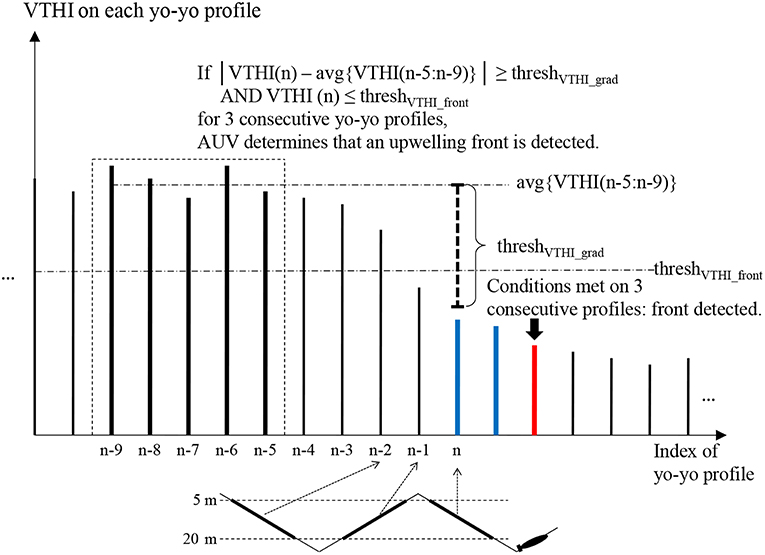
Figure 4. Illustration of the AUV front detection algorithm when flying from stratified water to upwelling water. The first two profiles that satisfy VTHI ≤ thresh_{VTHI_front} and the horizontal gradient (absolute value) of VTHI ≥ thresh_{VTHI_grad} are marked blue. The third such profile is marked red where the AUV determines front detection. Adapted from Zhang et al. (2012c) with permission.

The first deployment of this algorithm in an AUV sampling mission was in a frontal study in Monterey Bay on 13 June 2011. The Dorado AUV flew on a 31-km transect on latitude 36.9°N from an upwelling shadow region (stratified water column), through an upwelling front, into an upwelling water column. This latitude provided a relatively high probability of encountering strongly contrasting water types across an upwelling front (Zhang et al., 2012c), based on multi-year satellite SST and chlorophyll fluorescence line height data for the month of June that showed high horizontal gradients between the upwelling filament and the upwelling shadow (see Figures 3, 6). The vehicle ran on a yo-yo trajectory between the surface and 25-m depth (except for a small portion where the water depth was smaller than 33 m). The AUV's average horizontal speed was about 1 m/s. Its average vertical speed was about 0.15 m/s on descent profiles and 0.29 m/s on ascent profiles, respectively. The average horizontal distance spanned by one yo-yo profile was about 120 m.

Running the autonomous front detection algorithm, the AUV successfully classified the three distinct water types, accurately located the narrow front, and acquired targeted water samples from the three water types, as shown in Figure 5. The algorithm allocated the ten gulpers to the three types of water columns as follows: three in the stratified water, four in the upwelling front, and the remaining three in the upwelling water. More gulpers were allocated for the upwelling front because of high interest in studying plankton populations inside the front, and also because it was very hard to acquire water samples from the narrow front using traditional methods. Within the stratified water where phytoplankton populations formed dense patches, the AUV directed sampling by applying the peak-capture algorithm (Figure 1) to target the dense patches of planktonic organisms. After the AUV was recovered, the 10 water samples were analyzed using the sandwich hybridization assay (SHA) method (Scholin et al., 1999; Harvey et al., 2012) to measure zooplankton (mussels, barnacles, calanoid copepods, and podoplean copepods) RNA signals. The result (Zhang et al., 2012c) showed that mussel larvae, calanoid copepods, and podoplean copepods were most abundant in the stratified upwelling shadow region, where a subsurface phytoplankton layer was sampled. These organisms were not detected in the upwelling water column on the offshore side of the front. Calanoid copepods were moderately abundant in waters collected from the upwelling front. By integrating horizontal localization of physical features and vertical localization of biological features, targeted sampling capabilities enabled an AUV to autonomously conduct “surgical sampling” of a complex marine ecosystem.

FIGURE 5

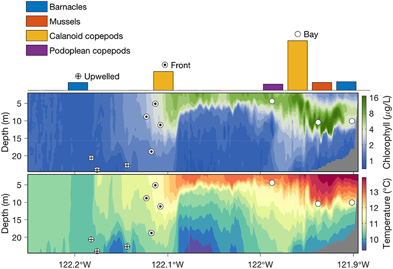
Figure 5. In the 2011 frontal sampling experiment in Monterey Bay, the Dorado AUV flew westward on a 31-km transect along 36.9°N, on a yo-yo trajectory from the surface to 25-m depth (except for a shallow-water portion near the east end of the transect). Chlorophyll fluorescence and temperature measured by the AUV are shown in the upper and lower panels, respectively. Locations of where the AUV's ten gulpers were triggered in the three distinct water columns are marked by the corresponding symbols. Zooplankton abundance in the water samples is shown by color-coded bars.

2.3. Tracking a Physical and Biological Front From Upwelling to Relaxation

Using the VTHI metric, we developed an AUV algorithm for tracking a stratification front (Zhang et al., 2012b) as it moves due to variations in wind and ocean circulation. Suppose an AUV starts from a strongly stratified water column (where VTHI is high), flying toward a weakly stratified water column (where VTHI is low) on a yo-yo trajectory. When VTHI falls below a threshold, the vehicle determines that it has passed the front and entered the weakly stratified water column. The AUV continues flight in the weakly stratified water for a certain distance so as to sufficiently survey the frontal zone and this water type, and then reverses course to fly back to the strongly stratified water. On this course, when VTHI rises above the threshold, the AUV determines that it has repassed the front and re-entered the strongly stratified water column. The AUV continues flight in this water type for a certain distance, and then reverses course to fly back to the weakly stratified water. To prevent false detection, the algorithm confirms front crossing only when VTHI satisfies the threshold on a certain number of consecutive yo-yo profiles. The AUV repeats the above cycle, thus effectively tracking the dynamic front.

In June 2012, a Tethys-class long-range AUV (LRAUV) (Bellingham et al., 2010; Hobson et al., 2012) ran this algorithm to study the evolution of a frontal zone in Monterey Bay through a period of variability in upwelling intensity (Zhang et al., 2015), as shown in Figure 6. The LRAUV flew on a yo-yo trajectory between the surface and 50 m depth on latitude 36.9°N. The vehicle's average horizontal speed was 0.9 m/s, and its average vertical speed was 0.24 m/s.

FIGURE 6

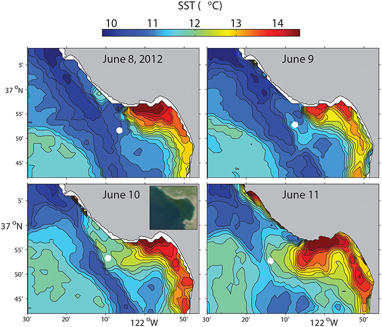
Figure 6. Satellite SST of Monterey Bay on 08-Jun 21:09, 09-Jun 22:30, 10-Jun 22:09, 11-Jun 21:48 (PDT), 2012. The circles mark the LRAUV-tracked front locations which were within 4 h of each SST acquisition time. Satellite ocean color at 10-Jun 12:54 (PDT) is shown in the inset in the lower-left panel. Reused from Zhang et al. (2015) with permission.

The LRAUV made 23 frontal crossings in 4 days, as shown in Figure 7. In the active upwelling phase from 8 to 10 June, an upwelling filament extended southeastward from the Point Año Nuevo upwelling center to the mouth of the bay (Figure 6). As shown in the left panel of Figure 7, the LRAUV tracked the front between the strongly stratified upwelling shadow water (on the inshore side) and the vertically homogenized upwelling filament (on the offshore side). In the relaxation phase from 10 to 12 June, the upwelling filament waned, and the upwelling shadow advanced westward for about 10 km to come in direct contact with the warmer coastal transition zone (CTZ) water [the CTZ refers to the zone between the near-shore upwelling region and the offshore California Current (Huyer et al., 1991)]. The LRAUV tracked the front between the strongly stratified upwelling shadow water (on the inshore side) and the weakly stratified CTZ water (on the offshore side). What enabled the LRAUV to stay with the stratification front through changing conditions was targeting the strong horizontal gradient of VTHI. On each instance of front detection, the vehicle adapted path (continuing flight for 4 km and then reversing course) to focus observations on the frontal zone.

FIGURE 7

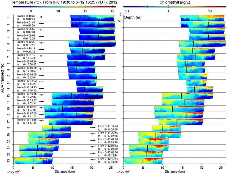
Figure 7. In the 2012 front tracking experiment in Monterey Bay, LRAUV-measured temperature (Left) and chlorophyll (Right) from the surface to 50 m depth on the 23 front-crossing transects. The vehicle's flight direction is indicated by the arrow (the inshore side is on the right). The LRAUV-tracked front location is marked by the vertical bar. The time range of each transect is also noted. Reused from Zhang et al. (2015) with permission.

The stratification front was also a persistent biological front between the strongly stratified phytoplankton-enriched water inshore of the front, and the weakly stratified phytoplankton-poor water offshore of the front (Figure 7). The biogeochemical nature of the water types to either side of the front changed in response to relaxation of upwelling. The most significant biogeochemical changes from the active upwelling phase to the relaxation phase were increased chlorophyll concentrations on the inshore side of the front (shown in the right panel of Figure 7) and associated increase in oxygen and decrease in nitrate (Zhang et al., 2015). This was consistent with enhanced productivity in the upwelling shadow during the relaxation response. The LRAUV front tracking provided an unprecedentedly detailed depiction of the frontal zone from active upwelling to relaxation.

2.4. Tracking and Sampling the Microbial Community in the Deep Chlorophyll Maximum Layer in an Open-Ocean Eddy

In the open ocean, photosynthesis is limited by low concentrations of nutrients in shallow water that receives the most sunlight. At the base of the nutrient impoverished surface layer (~100 m depth), nutrient concentrations increase across the strong density gradient of the pycnocline. This creates a vertically limited layer in which photosynthetic microbes can access both nutrients from below and light from above. With its locally enhanced concentration of the photosynthetic pigment chlorophyll, this layer is referred to as the deep chlorophyll maximum (DCM) (Huisman et al., 2006; Cullen, 2015). The DCM is a ubiquitous feature of open-ocean ecosystems.

Eddies alter the vertical distributions of nutrients and DCM microbial populations, thereby influencing the functioning of open-ocean ecosystems and global biogeochemical cycles (McGillicuddy, 2016). In cyclonic eddies (counterclockwise in the northern hemisphere), upward transport of nutrients and DCM populations enhances both nutrient and light resources for photosynthesis, resulting in increased productivity and biomass, and changes in species composition and export of organic matter to the deep sea (Vaillancourt et al., 2003; Brown et al., 2008).

Studies of how eddies influence open-ocean microbial populations have largely relied on ship-based sampling strategies. While this approach permits synoptic descriptions of eddies and microbial populations, it cannot provide effective sampling of DCM microbial populations in their natural frame of reference, which is moving with ocean currents (i.e., Lagrangian).

Horizontal and temporal variations of DCM depth tend to follow those of an isopycnal layer (Letelier et al., 1993; Karl et al., 2002). When density variation is dominated by temperature variation, an isopycnal can be effectively tracked by tracking an isotherm. We developed an algorithm to enable a Tethys-class LRAUV to autonomously track the DCM layer by locking onto the isotherm corresponding to the chlorophyll peak (Zhang et al., 2019a), and to sample the DCM layer using an autonomous robotic sampler designed as a payload in the LRAUV, the 3rd-generation ESP (3G-ESP) (Pargett et al., 2015; Scholin et al., 2017).

The autonomous isotherm finding and tracking algorithm is illustrated in Figure 8. It comprises three steps: (1) The AUV descends from the sea surface to a deep bound that is sufficiently deeper than the anticipated DCM depth. On the descent, the AUV finds the peak of the low-pass filtered chlorophyll fluorescence signal, and the corresponding temperature. (2) Once reaching the deep bound, the AUV turns to an ascent. (3) On the ascent, when the AUV reaches the chlorophyll-peak associated temperature, the vehicle stops ascending and thereafter actively adjusts its depth to remain at that temperature.

FIGURE 8

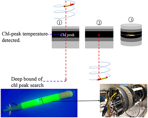
Figure 8. Illustration of the AUV algorithm for autonomously finding the DCM temperature and tracking that isotherm (Upper). The gray scale level represents the chlorophyll signal level. The darkest layer represents the DCM. The bottom photos [courtesy of Elisha Wood-Charlson (Left) and James Birch (Right)] show the LRAUV Aku equipped with a 3G-ESP in the fore-mid section.

In the March-April 2018 SCOPE (Simons Collaboration on Ocean Processes and Ecology) Hawaiian Eddy Experiment, the LRAUV Aku (carrying a 3G-ESP) (bottom photos in Figure 8) ran the algorithm to track and sample the DCM microbial community for 4 days in a cyclonic eddy to the northeast of Moloka'i (Zhang et al., 2019a). The vehicle ran on tight circles (circle radius ~10 m) at 1 m/s speed while drifting with the eddy current. The sampling permitted resolution of time-dependent change of the microbial assemblage in response to diel environmental variations.

Aku and a second LRAUV Opah as well as a Liquid Robotics Wave Glider Mola were each equipped with a Teledyne Benthos directional acoustic transponder (DAT) that integrates an acoustic modem and an ultra-short baseline (USBL) acoustic positioning system. Opah acoustically tracked Aku, while spiraling up and down between 50 and 200 m depths around Aku to measure the contextual water properties. The Wave Glider Mola also acoustically followed Aku to provide real-time tracking and the functionality of terminating Aku's mission. The three vehicles' tracks are shown in Figure 9. In the upper panel of Figure 10, Aku's depth trajectory (black line) is overlaid on Opah-measured contextual chlorophyll. The overlap of Aku's depth and Opah-measured chlorophyll-maximum depth confirms that Aku precisely tracked the DCM layer. In the lower panel, Aku's depth trajectory is overlaid on Opah-measured contextual temperature, which shows that Aku stayed on the targeted isotherm corresponding to the DCM. The large depth excursions on 1 April marked the transition to a different sampling mode, one designed to acquire a series of samples within, below and above the DCM layer. In 74 h of continuous tracking of the DCM layer, Aku drifted in the eddy current at an average drift speed of 0.27 m/s. This speed was consistent with the drift speed (0.27 m/s) of a GPS-tracked drifter (comprising a surface float and a drogue at 120 m depth) deployed near Aku, and R/V Falkor (near Aku's route) shipboard ADCP-measured Earth-referenced current velocity (0.25 m/s) at the 103-m depth bin (nearest DCM's mean depth of 105 m). The closeness between Aku's drift speed and that of the drifter as well as the ship ADCP-measured eddy current velocity shows that Aku followed the DCM water mass in a quasi-Lagrangian mode (Zhang et al., 2019a).

FIGURE 9

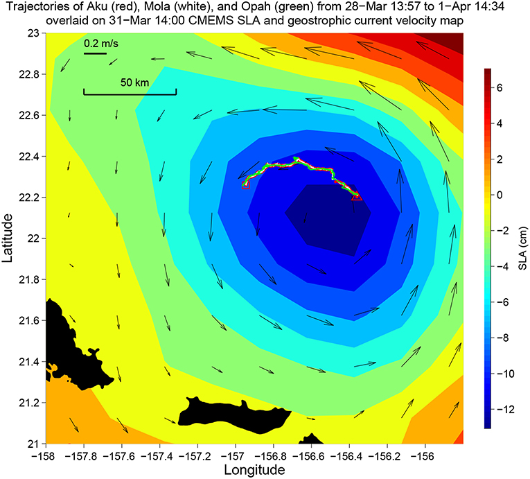
Figure 9. The trajectories of Aku, Opah, and Mola during Aku's 4-day sampling mission in the 2018 Hawaiian Eddy Experiment. Their trajectories are overlaid on the Copernicus Marine Environment Monitoring Service (CMEMS) sea level anomaly (SLA) and geostrophic current velocity map. The triangle and the square mark the start and the end of the mission, respectively. Time is in Hawaii Standard Time (HST).

FIGURE 10

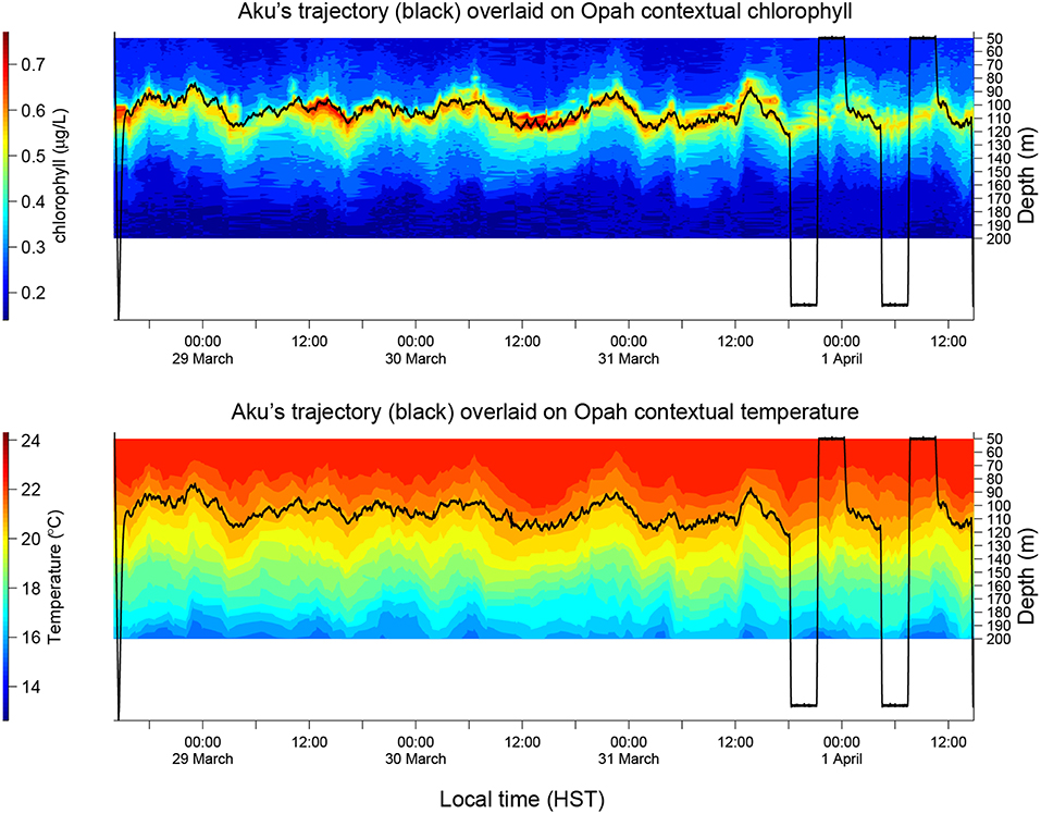
Figure 10. Aku's depth trajectory overlaid on Opah-measured contextual chlorophyll (Upper) and temperature (Lower), respectively, during Aku's 4-day sampling mission in the 2018 Hawaiian Eddy Experiment.

3. Conclusion and Future Work

By enabling AUVs to autonomously detect specific oceanic features and in turn adapt their behaviors, we are now able to reliably and effectively characterize targeted processes with greater flexibility than what is possible using manned vessels. The examples presented in this paper represent several cases that illustrate the utility of this approach, focusing on ecologically significant phenomena commonly observed in coastal and open-ocean settings. Vertical localization of subsurface phytoplankton layers enabled the detection and sampling of the historically most toxic algal populations in Monterey Bay, something that is not possible from routine monitoring at fixed locations. Horizontal localization applied to frontal habitats enabled allocation of discrete water sample collections across two end-member water types and the physical front between them. Where plankton populations formed dense patches within one of the three domains, vertical localization again enabled precise sampling of dense plankton patches. Combined with environmental sensor data, the molecular analyses of autonomously collected samples can provide a detailed, high-resolution view of the relationships between plankton and their pelagic habitat. Targeting the horizontal gradient of vertical stratification enabled an LRAUV to focus observations on a frontal zone from active upwelling to relaxation, which provided an unprecedentedly detailed depiction of the biogeochemical changes on both sides of the front during this transition.

The AUV algorithms can be extended to other mobile platforms under suitable conditions. For example, although a Wave Glider (Hine et al., 2009) can only make near-surface measurement, it can autonomously detect and track an upwelling front by taking advantage of the strong horizontal gradient of near-surface temperature, using an algorithm modified from the AUV algorithm (Zhang et al., 2019b).

In the 2018 SCOPE Hawaiian Eddy Experiment, multi-vehicle collaboration allowed continuous DCM sampling and contextual mapping in a moving eddy field, enabling a new mode of quasi-Lagrangian microbial ecology studies (Hobson et al., 2018). The water sampling LRAUV that stayed in the DCM layer was “near-sighted”—unaware of contextual water properties above and below the DCM layer. The mapping LRAUV provided this context by acoustically tracking the sampling LRAUV and spiraling up and down, yet there was no data exchange between them. In the future we will use inter-vehicle acoustic messaging to enable exchange of key information (e.g., chlorophyll level, vertical homogeneity). By exchanging complementary information of adjacent water columns, the collaborating AUVs can make timely adaptations of survey paths and behaviors in order to identify and concentrate on the most valuable targets.

Author Contributions

YZ, JR, BK, BH, BB, JGB, JMB, CS, and FC proposed and designed AUV targeted sampling methods. YZ, BK, RM, and MG developed AUV software. JH analyzed AUV water samples. All authors contributed to manuscript editing.

Funding

This work was supported by the David and Lucile Packard Foundation. The 2015 experiment in Monterey Bay was partially supported by NOAA Ecology and Oceanography of Harmful Algal Blooms (ECOHAB) Grant NA11NOS4780030. The 2018 SCOPE Hawaiian Eddy Experiment was partially supported by the National Science Foundation (OCE-0962032 and OCE-1337601), Simons Foundation Grant #329108, the Gordon and Betty Moore Foundation (Grant #3777, #3794, and #2728), and the Schmidt Ocean Institute for R/V Falkor Cruise FK180310. Publication of this paper was funded by the Schmidt Ocean Institute.

Conflict of Interest Statement

The authors declare that the research was conducted in the absence of any commercial or financial relationships that could be construed as a potential conflict of interest.

Acknowledgments

We thank J. Erickson, M. Chaffey, E. Mellinger, B. Raanan, M. J. Stanway, D. Klimov, and T. Hoover for contributions to the LRAUV development. We thank D. Pargett, C. Preston, B. Roman, K. Yamahara, W. Ussler, S. Jensen, and R. Marin III for contributions to the 3G-ESP development. We thank the MBARI Dorado AUV team lead H. Thomas for supporting tests of the targeted sampling software on the vehicle, team members D. Thompson, D. Conlin, and E. Martin for field operations, and K. Headley for helping setting up the onshore computer that runs simulation tests. For the 2011 and 2012 experiments in Monterey Bay, the satellite Advanced Very High Resolution Radiometer (AVHRR) SST data came from the National Oceanographic and Atmospheric Administration (NOAA) CoastWatch, and the regional ocean color data from the satellite Moderate Resolution Imaging Spectroradiometer (MODIS) sensor were obtained from the NASA LAADS system as Level 1A and processed to Level 3 mapped images using the SeaDAS software. For the 2018 Hawaiian Eddy Experiment, we are thankful for the contributions of MBARI colleagues T. O'Reilly, C. Rueda, K. Gomes, and University of Hawaii colleagues E. DeLong, D. Karl, A. Romano, S. Poulos, S. Wilson, G. Foreman, H. Ramm, A. White, F. Henderikx, R. Tabata, T. Burrell, E. Shimabukuro, T. Clemente, E. Firing, J. Hummon, P. Den Uyl, B. Watkins, E. Wood-Charlson, and L. Fujieki. The Hawaii SLA and geostrophic current velocity data came from the Copernicus Marine Environment Monitoring Service (CMEMS, http://marine.copernicus.eu/). We thank M. Salisbury for refining Figure 6 and M. Kelly for providing information about ship operations. We are thankful to D. Au for his support and advice. We are thankful for the help of R/V Zephyr crew in the Monterey Bay experiments and R/V Falkor crew in the Hawaii experiment. We appreciate the very helpful comments from the three reviewers for improving the paper.

Footnote

1. ^Research vessel daily operational cost ranges from $20,000 to $60,000.

References

Barber, R., and Smith, R. L. (1981). “Coastal upwelling ecosystems,” in Analysis of Marine Ecosystems, ed A. R. Longhurst (London: Academic Press), 31–68.

Google Scholar

Bellingham, J. G., Zhang, Y., Kerwin, J. E., Erikson, J., Hobson, B., Kieft, B., et al. (2010). “Efficient propulsion for the Tethys long-range autonomous underwater vehicle,” in Proceedings of IEEE AUV'2010 (Monterey, CA), 1–6.

Google Scholar

Billings, A., Kaiser, C., Young, C. M., Hiebert, L. S., Cole, E., Wagner, S. J. K., et al. (2017). SyPRID sampler: a large-volume, high-resolution, autonomous, deep-ocean precision plankton sampling system. Deep Sea Res. II 137, 297–306. doi: 10.1016/j.dsr2.2016.05.007

CrossRef Full Text | Google Scholar

Brown, S. L., Landry, M. R., Selph, K. E., Yang, E. J., Rii, Y. M., and Bidigare, R. R. (2008). Diatoms in the desert: plankton community response to a mesoscale eddy in the subtropical North Pacific. Deep Sea Res. II 137, 1321–1333. doi: 10.1016/j.dsr2.2008.02.012

CrossRef Full Text | Google Scholar

Camilli, R., Reddy, C. M., Yoerger, D. R., Mooy, B. A. S. V., Jakuba, M. V., Kinsey, J. C., et al. (2010). Tracking hydrocarbon plume transport and biodegradation at Deepwater Horizon. Science 330, 201–204. doi: 10.1126/science.1195223

PubMed Abstract | CrossRef Full Text | Google Scholar

Cazenave, F., Zhang, Y., McPhee-Shaw, E., Bellingham, J. G., and Stanton, T. (2011). High-resolution surveys of internal tidal waves in Monterey Bay, California, using an autonomous underwater vehicle. Limnol. Oceanogr. Methods 9, 571–581. doi: 10.4319/lom.2011.9.571

CrossRef Full Text | Google Scholar

Cowles, T. J., Desiderio, R. A., and Carr, M.-E. (1998). Small-scale planktonic structure: persistence and trophic consequences. Oceanography 11, 4–9. doi: 10.5670/oceanog.1998.08

CrossRef Full Text | Google Scholar

Cruz, N., and Matos, A. C. (2010a). “Adaptive sampling of thermoclines with autonomous underwater vehicles,” in Proceeding of MTS/IEEE Oceans'10 (Seattle, WA), 1–6.

Google Scholar

Cruz, N., and Matos, A. C. (2010b). “Reactive AUV motion for thermocline tracking,” in Proceeding of IEEE Oceans'10 (Sydney), 1–6.

Google Scholar

Cullen, J. J. (2015). Subsurface chlorophyll maximum layers: enduring enigma or mystery solved? Annu. Rev. Mar. Sci. 7, 207–239. doi: 10.1146/annurev-marine-010213-135111

CrossRef Full Text | Google Scholar

Farrell, J. A., Pang, S., and Li, W. (2005). Chemical plume tracing via an autonomous underwater vehicle. IEEE J. Ocean. Eng. 30, 428–442. doi: 10.1109/JOE.2004.838066

CrossRef Full Text | Google Scholar

German, C. R., Yoerger, D. R., Jakuba, M., Shank, T. M., Langmuir, C. H., and Nakamura, K.-I. (2008). Hydrothermal exploration with the Autonomous Benthic Explorer. Deep Sea Res. I 55, 203–219. doi: 10.1016/j.dsr.2007.11.004

CrossRef Full Text | Google Scholar

Govindarajan, A. F., Pineda, J., Purcell, M., and Breier, J. A. (2015). Species- and stage-specific barnacle larval distributions obtained from AUV sampling and genetic analysis in Buzzards Bay, Massachusetts, USA. J. Exp. Mar. Biol. Ecol. 472, 158–165. doi: 10.1016/j.jembe.2015.07.012

CrossRef Full Text | Google Scholar

Graham, W. M., Field, J. G., and Potts, D. C. (1992). Persistent “upwelling shadows” and their influence on zooplankton distributions. Mar. Biol. 114, 561–570. doi: 10.1007/BF00357253

CrossRef Full Text | Google Scholar

Graham, W. M., and Largier, J. L. (1997). Upwelling shadows as nearshore retention sites: the example of northern Monterey Bay. Contin. Shelf Res. 17, 509–532. doi: 10.1016/S0278-4343(96)00045-3

CrossRef Full Text | Google Scholar

Harvey, J. B. J., Ryan, J. P., Marin, R. III., Preston, C. M., Alvarado, N., Scholin, C. A., et al. (2012). Robotic sampling, in situ monitoring and molecular detection of marine zooplankton. J. Exp. Mar. Biol. Ecol. 413, 60–70. doi: 10.1016/j.jembe.2011.11.022

CrossRef Full Text | Google Scholar

Hine, R., Willcox, S., Hine, G., and Richardson, T. (2009). “The wave glider: a wave-powered autonomous marine vehicle,” in Proceedings of MTS/IEEE Oceans'09 (Biloxi, MS), 1–6.

Google Scholar

Hobson, B., Bellingham, J. G., Kieft, B., McEwen, R., Godin, M., and Zhang, Y. (2012). “Tethys-class long range AUVs - extending the endurance of propeller-driven cruising AUVs from days to weeks,” in Proceedings of IEEE AUV'2012 (Southampton, UK), 1–8.

Google Scholar

Hobson, B., Kieft, B., Raanan, B., Zhang, Y., Birch, J., Ryan, J. P., et al. (2018). “An autonomous vehicle based open ocean Lagrangian observatory,” in Proceedings of IEEE AUV'2018 (Porto), 1–5.

Google Scholar

Huisman, J., Pham Thi, N., Karl, D. M., and Sommeijer, B. (2006). Reduced mixing generates oscillations and chaos in the oceanic deep chlorophyll maximum. Nature 439:322–325. doi: 10.1038/nature04245

PubMed Abstract | CrossRef Full Text | Google Scholar

Huyer, A., Kosro, P. M., Fleischbein, J., Ramp, S. R., Stanton, T., Washburn, L., et al. (1991). Currents and water masses of the coastal transition zone off northern California, June to August 1988. J. Geophys. Res. 96, 14809–14831. doi: 10.1029/91JC00641

CrossRef Full Text | Google Scholar

Karl, D. M., Bidigare, R. R., and Letelier, R. M. (2002). “Chapter 2: Sustained and aperiodic variability in organic matter production and phototrophic microbial community structure in the North Pacific Subtropical Gyre,” in Phytoplankton Productivity: Carbon Assimilation in Marine and Freshwater Ecosystems, eds P. J. le B. Williams, D. N. Thomas, and C. S. Reynolds (Osney Mead, UK: Blackwell Science Ltd), 222–264.

Google Scholar

Kukulya, A. L., Bellingham, J. G., Stokey, R. P., Whelan, S. P., Reddy, C. M., Conmy, R. N., et al. (2018). Autonomous chemical plume detection and mapping demonstration results with a COTS AUV and sensor package. Proceedings of MTS/IEEE Oceans'18 (Charleston, SC), 1–6.

Google Scholar

Lasker, R. (1975). Field criteria for survival of anchovy larvae: the relation between inshore chlorophyll maximum layers and successful first feeding. Fish. Bull. 73, 453–462.

Google Scholar

Letelier, R. M., Bidigare, R. R., Hebel, D. V., Ondrusek, M., Winn, C. D., and Karl, D. M. (1993). Temporal variability of phytoplankton community structure based on pigment analysis. Limnol. Oceanogr. 38, 1420–1437. doi: 10.4319/lo.1993.38.7.1420

CrossRef Full Text | Google Scholar

McGillicuddy, D. J. (2016). Mechanisms of physical-biological-biogeochemical interaction at the oceanic mesoscale. Annu. Rev. Mar. Sci. 8, 125–159. doi: 10.1146/annurev-marine-010814-015606

PubMed Abstract | CrossRef Full Text | Google Scholar

McManus, M. A., Kudela, R. M., Silver, M. W., Steward, G. F., Donaghay, P. L., and Sullivan, J. M. (2008). Cryptic blooms: are thin layers the missing connection? Estuar. Coasts 31, 396–401. doi: 10.1007/s12237-007-9025-4

CrossRef Full Text | Google Scholar

Paduan, J. B., Zierenberg, R. A., Clague, D. A., Spelz, R. M., Caress, D. W., Troni, G., et al. (2018). Discovery of hydrothermal vent fields on Alarcón Rise and in Southern Pescadero Basin, Gulf of California. Geochem. Geophys. Geosyst. 19, 4788–4819. doi: 10.1029/2018GC007771

CrossRef Full Text | Google Scholar

Pargett, D. M., Birch, J. M., Preston, C. M., Ryan, J. P., Zhang, Y., and Scholin, C. A. (2015). “Development of a mobile ecogenomic sensor,” in Proceedings of MTS/IEEE Oceans'15 (Washington, DC), 1–6.

Google Scholar

Petillo, S., Balasuriya, A., and Schmidt, H. (2010). “Autonomous adaptive environmental assessment and feature tracking via autonomous underwater vehicles” in Proceedings of IEEE Oceans'10 (Sydney), 1–9.

Google Scholar

Petillo, S., and Schmidt, H. (2014). Exploiting adaptive and collaborative AUV autonomy for detection and characterization of internal waves. IEEE J. Ocean. Eng. 39, 150–164. doi: 10.1109/JOE.2013.2243251

CrossRef Full Text | Google Scholar

Ryan, J. P., Fischer, A. M., Kudela, R. M., McManus, M. A., Myers, J. S., Paduan, J. D., et al. (2010b). Recurrent frontal slicks of a coastal ocean upwelling shadow. J. Geophys. Res. 115:C12070. doi: 10.1029/2010JC006398

CrossRef Full Text | Google Scholar

Ryan, J. P., Harvey, J. B. J., Zhang, Y., and Woodson, C. B. (2014). Distributions of invertebrate larvae and phytoplankton in a coastal upwelling system retention zone and peripheral front. J. Exp. Mar. Biol. Ecol. 459, 51–60. doi: 10.1016/j.jembe.2014.05.017

CrossRef Full Text | Google Scholar

Ryan, J. P., Johnson, S. B., Sherman, A., Rajan, K., Py, F., Thomas, H., et al. (2010a). Mobile autonomous process sampling within coastal ocean observing systems. Limnol. Oceanogr. Methods 8, 394–402. doi: 10.4319/lom.2010.8.394

CrossRef Full Text | Google Scholar

Ryan, J. P., Kudela, R. M., Birch, J. M., Blum, M., Bowers, H. A., Chavez, F. P., et al. (2017). Causality of an extreme harmful algal bloom in Monterey Bay, California, during the 2014–2016 northeast Pacific warm anomaly. Geophys. Res. Lett. 44, 1–9. doi: 10.1002/2017GL072637

CrossRef Full Text | Google Scholar

Ryan, J. P., McManus, M. A., Paduan, J. D., and Chavez, F. P. (2008). Phytoplankton thin layers caused by shear in frontal zones of a coastal upwelling system. Mar. Ecol. Prog. Ser. 354, 21–34. doi: 10.3354/meps07222

CrossRef Full Text | Google Scholar

Ryan, J. P., McManus, M. A., and Sullivan, J. M. (2010c). Interacting physical, chemical and biological forcing of phytoplankton thin-layer variability in Monterey Bay, California. Contin. Shelf Res. 30, 7–16. doi: 10.1016/j.csr.2009.10.017

CrossRef Full Text | Google Scholar

Scholin, C., Birch, J., Jensen, S., Marin, R. III., Massion, E., Pargett, D., et al. (2017). The quest to develop ecogenomic sensors: a 25-year history of the Environmental Sample Processor (ESP) as a case study. Oceanography 30, 100–113. doi: 10.5670/oceanog.2017.427

CrossRef Full Text | Google Scholar

Scholin, C., Marin, R. III., Miller, P., Doucette, G., Powell, C., Howard, J., et al. (1999). Application of DNA probes and a receptor binding assay for detection of Pseudo-nitzschia (Bacillariophyceae) species and domoic acid activity in cultured and natural samples. J. Phycol. 35, 1356–1367.

Google Scholar

Scholin, C. A. (2013). "Ecogenomic sensors," in Encyclopedia of Biodiversity, 2nd Edn, Vol. 2, ed S. A. Levin (Waltham, MA: Academic Press),690–700.

Google Scholar

Smith, R. L. (1981). “A comparison of the structure and variability of the flow field in three coastal upwelling regions: Oregon, Northwest Africa, and Peru,” in Coastal Upwelling, ed F. A. Richards (Washington, DC: American Geophysical Union), 107–118.

Google Scholar

Sullivan, J. M., McManus, M. A., Cheriton, O. M., Benoit-Bird, K. J., Goodman, L., Wang, Z., et al. (2010). Layered organization in the coastal ocean: an introduction to planktonic thin layers and the LOCO project. Contin. Shelf Res. 30, 1–6. doi: 10.1016/j.csr.2009.09.001

CrossRef Full Text | Google Scholar

Vaillancourt, R. D., Marra, J., Seki, M. P., Parsons, M. L., and Bidigare, R. R. (2003). Impact of a cyclonic eddy on phytoplankton community structure and photosynthetic competency in the subtropical North Pacific Ocean. Deep Sea Res. I 50, 829–847. doi: 10.1016/S0967-0637(03)00059-1

CrossRef Full Text | Google Scholar

Woodson, C. B., Washburn, L., Barth, J. A., Hoover, D. J., Kirincich, A. R., McManus, M. A., et al. (2009). Northern Monterey Bay upwelling shadow front: observations of a coastally and surface-trapped buoyant plume. J. Geophys. Res. 114:C12013. doi: 10.1029/2009JC005623

CrossRef Full Text | Google Scholar

Wulff, T., Bauerfeind, E., and von Appen, W.-J. (2016). Physical and ecological processes at a moving ice edge in the Fram Strait as observed with an AUV. Deep Sea Res. I 115, 253–264. doi: 10.1016/j.dsr.2016.07.001

CrossRef Full Text | Google Scholar

Zhang, Y., Bellingham, J. G., Godin, M. A., and Ryan, J. P. (2012a). Using an autonomous underwater vehicle to track the thermocline based on peak-gradient detection. IEEE J. Ocean. Eng. 37, 544–553. doi: 10.1109/JOE.2012.2192340

CrossRef Full Text | Google Scholar

Zhang, Y., Bellingham, J. G., Ryan, J. P., and Godin, M. A. (2015). Evolution of a physical and biological front from upwelling to relaxation. Contin. Shelf Res. 108, 55–64. doi: 10.1016/j.csr.2015.08.005

CrossRef Full Text | Google Scholar

Zhang, Y., Godin, M. A., Bellingham, J. G., and Ryan, J. P. (2012b). Using an autonomous underwater vehicle to track a coastal upwelling front. IEEE J. Ocean. Eng. 37, 338–347. doi: 10.1109/JOE.2012.2197272

CrossRef Full Text | Google Scholar

Zhang, Y., Kieft, B., Hobson, B., Ryan, J., Barone, B., Preston, C., et al. (2019a). Autonomous tracking and sampling of the deep chlorophyll maximum layer in an open-ocean eddy by a long range autonomous underwater vehicle. IEEE J. Ocean. Eng. doi: 10.1109/JOE.2019.2920217

CrossRef Full Text | Google Scholar

Zhang, Y., McEwen, R. S., Ryan, J. P., and Bellingham, J. G. (2010). Design and tests of an adaptive triggering method for capturing peak samples in a thin phytoplankton layer by an autonomous underwater vehicle. IEEE J. Ocean. Eng. 35, 785–796. doi: 10.1109/JOE.2010.2081031

CrossRef Full Text | Google Scholar

Zhang, Y., McEwen, R. S., Ryan, J. P., Bellingham, J. G., Thomas, H., Thompson, C. H., et al. (2011). A peak-capture algorithm used on an autonomous underwater vehicle in the 2010 Gulf of Mexico oil spill response scientific survey. J. Field Robot. 28, 484–496. doi: 10.1002/rob.20399

CrossRef Full Text | Google Scholar

Zhang, Y., Rueda, C., Kieft, B., Ryan, J. P., Wahl, C., O'Reilly, T. C., et al. (2019b). Autonomous tracking of an oceanic thermal front by a wave glider. J. Field Robot. 36, 940–954. doi: 10.1002/rob.21617

CrossRef Full Text | Google Scholar

Zhang, Y., Ryan, J. P., Bellingham, J. G., Harvey, J. B. J., and McEwen, R. S. (2012c). Autonomous detection and sampling of water types and fronts in a coastal upwelling system by an autonomous underwater vehicle. Limnol. Oceanogr. Methods 10, 934–951. doi: 10.4319/lom.2012.10.934

CrossRef Full Text | Google Scholar