Observing the Oceans Acoustically

Introduction

The mesoscale revolution in oceanography was enabled by the acoustic tracking of floats. In the late 1950s, John Swallow and his colleagues deployed floats off Bermuda, returning a few weeks later to locate them acoustically. They expected them to have drifted only kilometers—but the floats had disappeared. When deploying the next set, they stayed and tracked them. Rather than moving slowly in one direction, as originally expected, they moved at relatively high speeds in random directions. It was from this study that mesoscale eddies were discovered (Crease, 1962; Swallow, 1971).

Marine mammals depend on acoustics in very fundamental ways, but this was not known early on. In the 1950s, classified navy surveillance systems heard many signals of unknown origin, including 20 Hz pulses or BLIPs (from the paper strip chart recorders) that were observed to be highly repetitive, point sources traveling at 1–4 knots. Various interpretations ranged from mechanical and geophysical sources to the breathing or heartbeat of a whale. Finally, in 1963, they were attributed to finback whale courtship displays (Schevill et al., 1964; Tavolga, 2012). This was but one step in revealing the rich babel of life in the ocean.

Since then float tracking and marine mammal studies have been major applications of acoustics in oceanography, with improvements along the way. As Watkins (1981) said, “The sounds from finback whales (Schevill et al., 1964) provided the stimulus for much of the early progress in design of equipment and techniques for the acoustic observations at sea.” Ever more acoustic tools were developed, including long-baseline positioning (∼10 km, originally to support drillship dynamic positioning), inverted and bio-acoustic echosounders, and acoustic doppler profilers. Early autonomous underwater vehicles (AUVs), and mobile platforms in general in the 1990s, motivated more work on combined positioning and communication and miniaturized sensors. A mix of acoustic and non-acoustic tools were developed to directly measure the ocean and also to provide necessary support infrastructure.

Ocean acoustic tomography as proposed by Munk and Wunsch (1982) catalyzed new directions. Many process experiments have amply demonstrated the concepts [measuring sound speed (temperature) and currents, N² growth of information with number of instruments], technology (broadband low frequency sources, precise timing and positioning, and coherent signal processing enabling precise travel time determination), and utility for measuring coastal, meso- and larger scale ocean variability (heat content changes, vorticity, baroclinic tides, deep ocean convection, to name a few). A defining event was the Acoustic Thermometry of Ocean Climate (ATOC) project (1996–2006), that demonstrated and served as a pilot for a basin scale ocean heat content observing system (with cabled instrumentation), and catalyzed new efforts in ocean bio-acoustics and passive acoustic monitoring (PAM). The latter includes more than bio-acoustics, with wind, rain, ice, earthquakes, volcanoes, and anthropogenic sound. Throughout, ocean data assimilation techniques struggle to accommodate the new data types and large amount of data generated.

The hydroacoustic monitoring component of the global Comprehensive Nuclear-Test-Ban Treaty Organization International Monitoring System (CTBTO IMS) has been in operation in the Indian Ocean since 2000. The original and primary purpose of the CTBTO IMS is to monitor for signals related to unsanctioned nuclear activity, but the scientific value of the recordings has been demonstrated in numerous studies related to ocean ambient sound, marine mammal behavior, glacial/iceberg noise, human ocean use, tsunami warning, and search and rescue.

These developments—ocean tomography and attendant technology, PAM, mobile platforms, and data assimilation—motivated ideas about regional (and together global) tomography systems (for the OceanObs99 conference; Dushaw et al., 2001), integrated acoustic systems for ocean observing (Howe and Miller, 2004), global ocean acoustic observing network (for OceanObs09 conference; Dushaw et al., 2009), and multipurpose acoustic networks in the integrated Arctic Ocean observing system (Mikhalevsky et al., 2015).

The vision we present in this paper is of a multi-purpose acoustic ocean observing system where the sum is greater than the individual parts. It is the network formed by the parts that yield the gains, both in terms of raw number of data but also the ocean information gain. The individual parts or components—sources, receivers, platforms—can all be shared among the various applications, including PAM, undersea and under-ice mobile platform positioning, navigation and communication, tomography, and more, including cost (Figures 1, 2). Each individual dataset then increases in value within a global context. Because acoustic instrumentation is in general robust and scalable, it is well suited for sustained, long term, multi-scale deployment as part of the Global Ocean Observing System (GOOS).

FIGURE 1

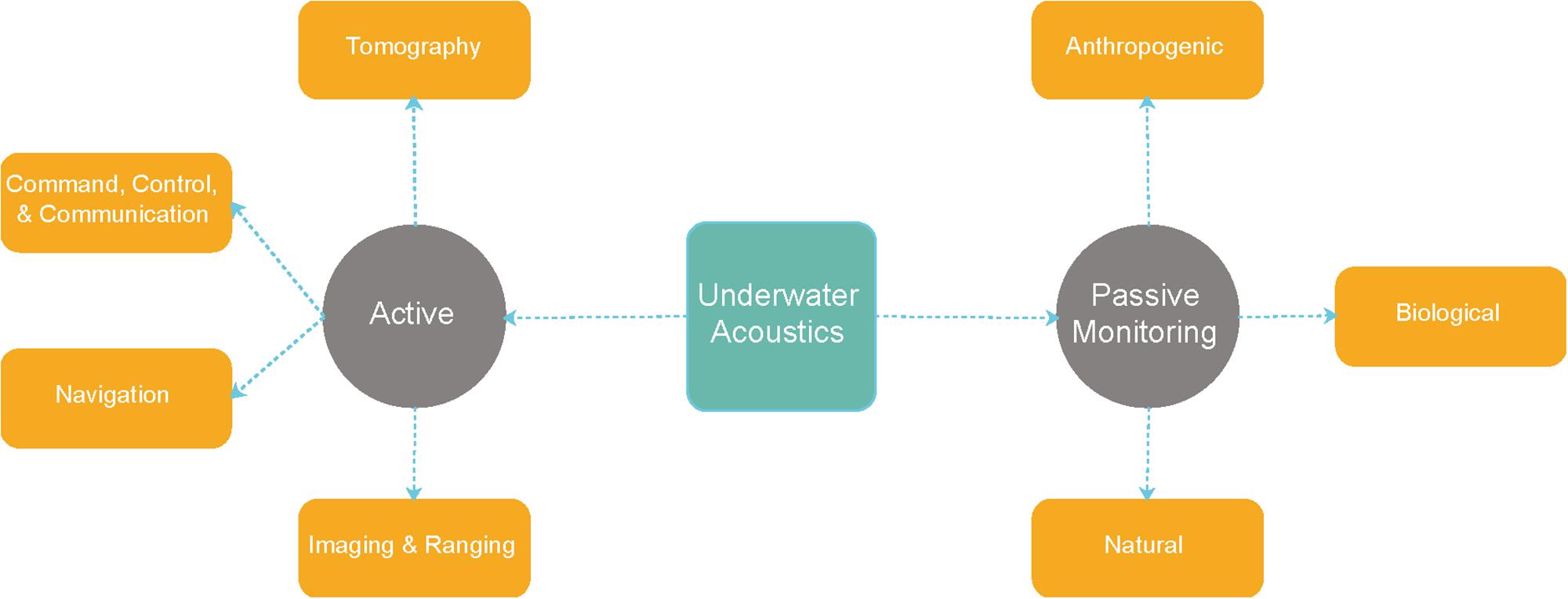
Figure 1. Key core elements of a multipurpose acoustic system for ocean observing (Figure provided by E. Rehm, used with permission).

FIGURE 2

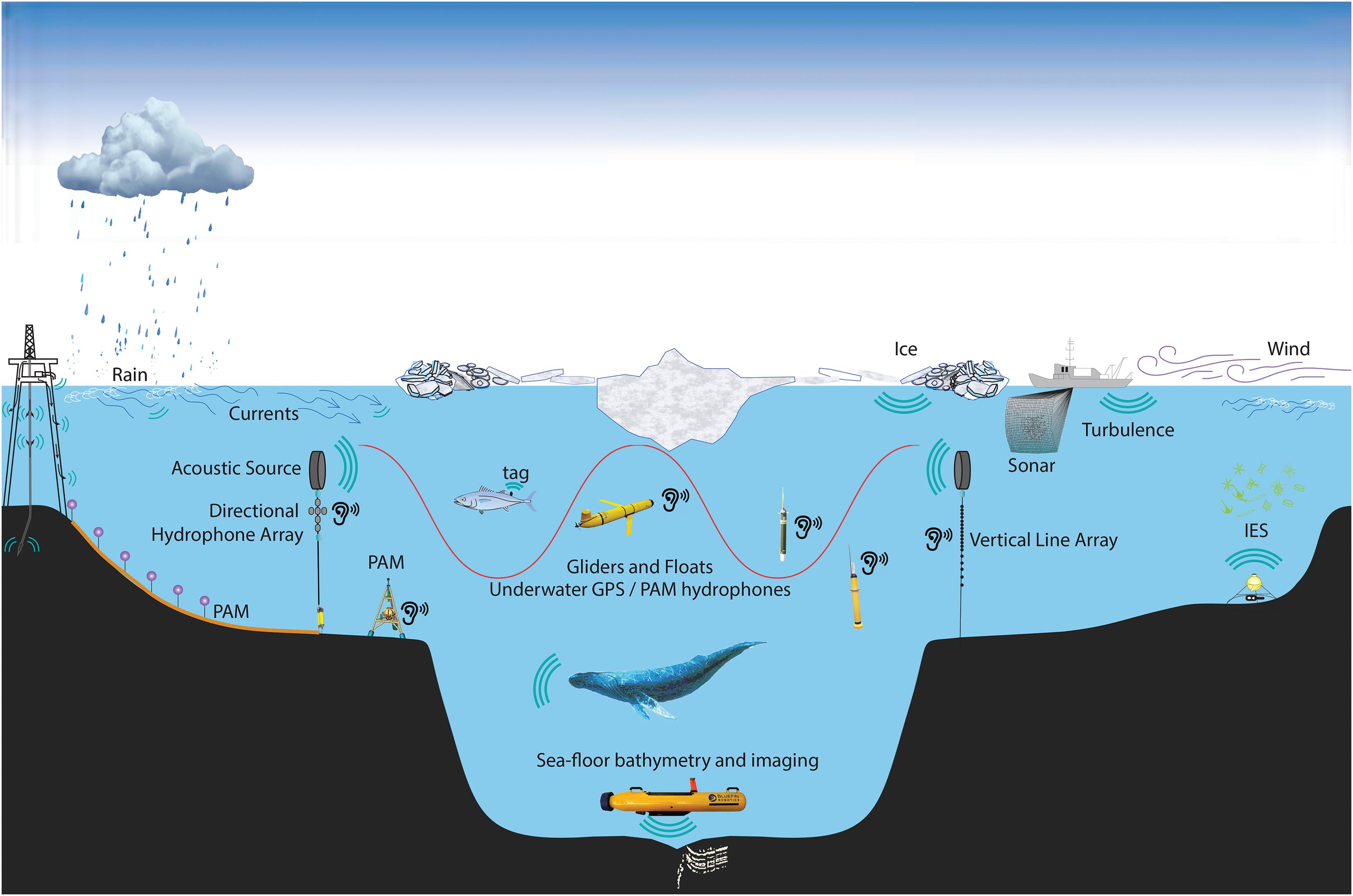
Figure 2. A multipurpose acoustic observing system provides a range of capabilities: two-way transceivers provide support for low-frequency acoustic tomography (heat content, averaged currents), navigation, and communications as well as broadband passive acoustic listening posts. Bottom-mounted passive acoustic monitoring (PAM) stations provide additional coverage for observing soundscapes of natural (wind, rain, ice), biological (plankton, fish, marine mammals), and anthropogenic (ships, sonar, drilling platform) sources. The shifting paths of ocean currents and zooplankton populations can be detected using inverted echo sounders (IES). Autonomous platforms (floats, glides) take advantage of acoustic sources providing “underwater GPS” services and can also provide PAM services. (Figure provided by E. Rehm, used with permission).

The goal of this OceanObs19 community white paper is to provide evidence to the readers and conference attendees that such a multi-purpose acoustic ocean observing system is an achievable component of GOOS that will bring many benefits.

A major outcome of the OceanObs09 conference was the Framework for Ocean Observing (Lindstrom et al., 2014). This document outlined the overall goals, objectives, structures, and processes of the GOOS. These include requirements that GOOS must: (1) serve multiple users/requirements with the same observing system; (2) make sustained observations over time with global-scale coverage; (3) be driven by end-user requirements; (4) incorporate continual evaluation, feedback and re-evaluation of system; (5) execute a phased implementation of components (concept/pilot/mature) based on technical readiness levels, and essential ocean variables with high feasibility and impact.

“Ocean Sound” has just been accepted by the Biology and Ecosystem Panel of GOOS as a mature Essential Ocean Variable (EOV; see Ocean Sound EOV, 2018). This is an important milestone primarily addressing PAM. This recognizes the technical readiness, feasibility, high impacts, and operational status of systems already in place. The latter is especially important and is reflected in the long-established operational global array of hydroacoustic stations as part of the CTBTO IMS (Figure 3). Further, there are many additional ongoing regional programs, including the ALOHA Cabled Observatory (ACO), NEPTUNE in the northeast Pacific, Perennial Acoustic Observatory in the Antarctic Ocean (PALAOA), and NOAA Ocean Noise Reference Station Network. There are a number of challenges, though, including: sustained funding for acoustic data management and network or system components; making ocean sound measurement ubiquitous on “integrated instrument packages” meant for broad deployment; integrated data management (easy access to any and all data—a “big data” problem); and broadening the scope to more explicitly include geophysical variables such as wind, rain, T-phase/earthquake/tsunami detections. For the purposes of a multi-purpose acoustic observing system, with positioning/tomography integral components thereof, it is important to require that receivers have adequate timing and positioning accuracy (1 ms and 1 m).

FIGURE 3

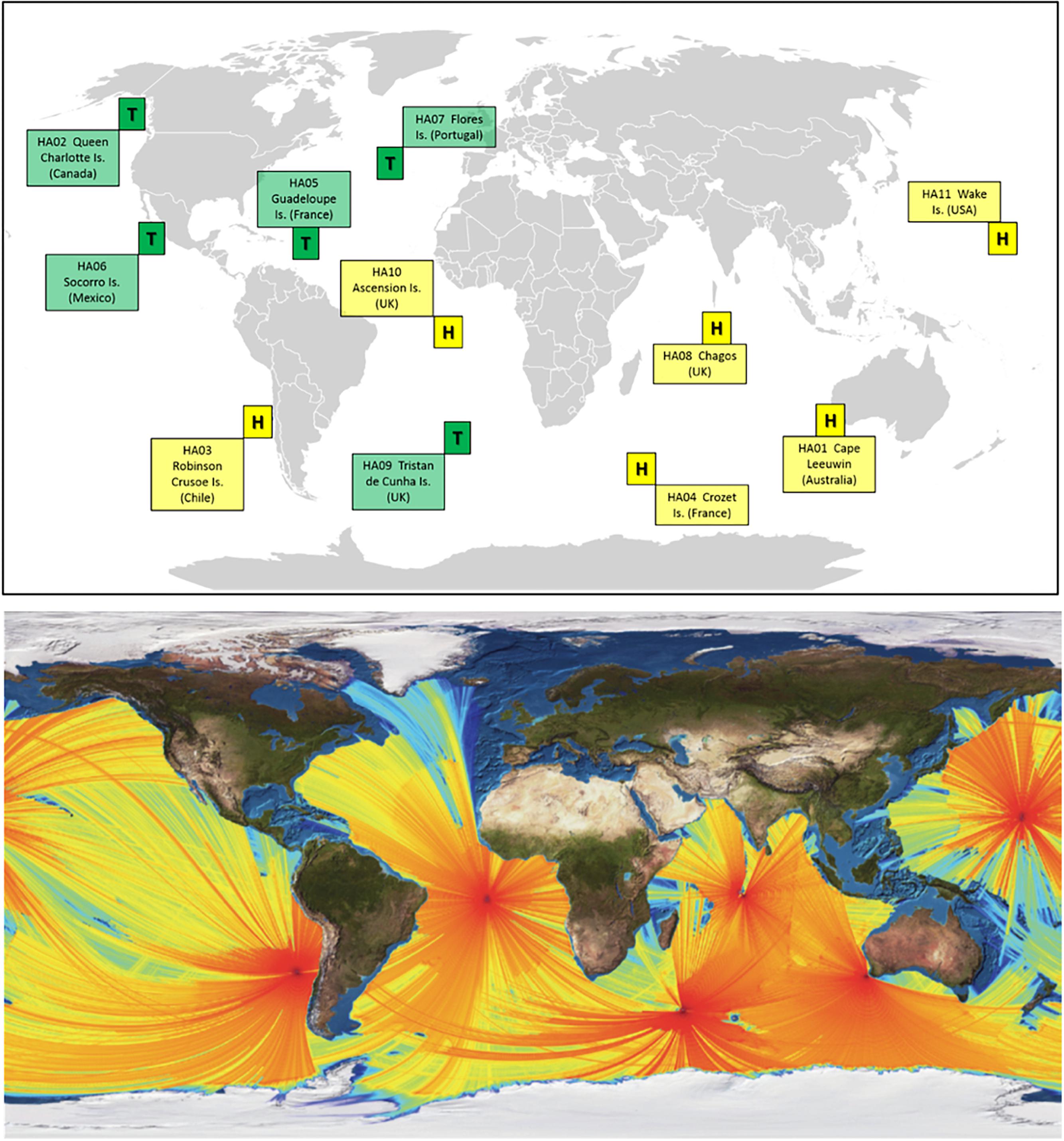
Figure 3. The CTBTO as a global acoustic receiving array, sensitive to many anthropogenic sounds. (Top) A world map showing the Comprehensive Nuclear-Test-Ban Treaty Organization International Monitoring System (CTBTO IMS) hydroacoustic component. Cabled hydrophone stations (1–100 Hz) are represented by the letter “H”, while T-stations (seismometers) are represented by the letter “T” (Haralabus et al., 2017). (Bottom) Modeled low frequency (<100 Hz) acoustic coverage of the CTBTO IMS hydrophone H-stations (Heaney, 2015, used with permission).

Other existing EOVs will directly benefit from measurements from multi-purpose acoustic systems. These include: EOV Subsurface Temperature from acoustic tomography; EOV Subsurface Velocity from acoustic tomography and mobile platform tracking; EOV Sea State from ocean sound/wind; EOV Marine Turtles, Birds, Mammals Abundance and Distribution from fixed and autonomous PAM sensors; EOV Zooplankton Biomass and Diversity in high-latitude marginal ice zones from mobile platform (float, glider) tracking.

In the balance of the paper, we begin with a review of acoustic technology and its capabilities, emphasizing the aspects that are important to the multipurpose nature of the acoustic observing system. To address the OceanObs19 Observing Needs themes, we have sections on discovery, ecosystems, climate and variability, and hazards and maritime safety. This is followed by a discussion that synthesizes the preceding sections. Concluding remarks and recommendations are given in the final section.

Observing Technology and Network

Multipurpose Acoustic Systems

Multipurpose acoustic networks directly provide unique observations while supporting and complementing other in situ observations – all are needed for a complete GOOS. Acoustic tomography provides observations of large-scale temperature and current. PAM records sounds generated by marine life, ice, earthquakes, volcanoes, wind (e.g., Vagle et al., 1990), rain (e.g., Nystuen, 2001), and other natural sources, as well as by anthropogenic sources such as ships and seismic air gun arrays. In a multipurpose acoustic system, PAM instruments will also record the signals from acoustic sources used for acoustic tomography and undersea positioning and navigation. Acoustic networks facilitate underwater and under-ice geo-positioning of floats, gliders, and other autonomous vehicles. Figure 4 illustrates the various applications (an elaboration of Figure 2).

FIGURE 4

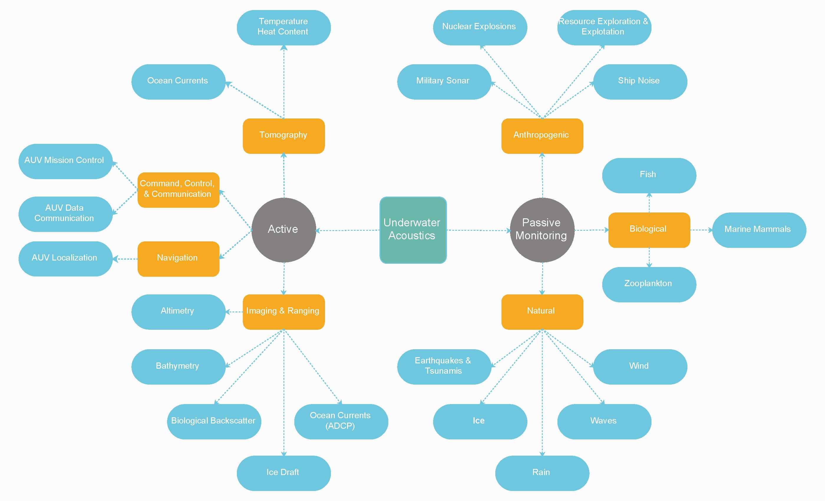
Figure 4. Ocean observing applications of a multipurpose acoustic system, building on the core elements. (Figure provided by E. Rehm, used with permission).

It is important to appreciate the network aspects that typically are involved in acoustics systems. In many cases, multiple receivers will record multiple sources, both natural and anthropogenic. As an example, data from a number of widely spaced PAM receivers could be used to simultaneously track a pod of blue whales, monitor volcanic activity along a mid-ocean ridge, and record transmissions from several acoustic sources to measure the temperature field. If desired, AUVs from a cabled docking station could be diverted from their routine mapping to monitor the ridge activity, using the acoustic positioning signals for locating themselves and navigating in real time (Figure 2).

Receiver and source technologies are mature, available, and ready for integration into an ocean observing system (e.g., Worcester et al., 2009; Morozov et al., 2016). The technology provides the required accuracy for tomography and underwater geo-positioning systems, as well as recordings of ambient sound and acoustic backscatter from the water column. Passive and active acoustic sensors are available for different frequency bands and different observing platforms, e.g., moorings, floats, bottom landers, and cabled systems. Passive systems can be quite broadband. The High-frequency Acoustic Recording Package (HARP), for example, has a bandwidth of 10–100,000 Hz (Wiggins and Hildebrand, 2007). Acoustic sources with center frequencies ranging from 20 Hz (Mikhalevsky and Gavrilov, 2001) to several kHz (e.g., Send et al., 2002) have been used in acoustic tomography experiments, depending on the range and application.

Tomographic Instrumentation and Signal Processing

The low-frequency acoustic source technology used to make large-scale tomographic measurements has advanced significantly in recent years. The bottom-mounted, cable-connected, 75-Hz ATOC sources deployed during the 1990s in the mid-latitude North Pacific Ocean were large and heavy (∼5000 kg) (ATOC Instrumentation Group, 1994). The autonomous acoustic sources used to generate the ∼20 Hz signals needed to propagate for long ranges under the ice in the Arctic Ocean for the Trans-Arctic Propagation (TAP) experiment in 1994 and the Acoustic Climate Observations using Underwater Sound (ACOUS) project beginning in 1999 were one-of-a-kind, large devices (Mikhalevsky and Gavrilov, 2001). With the dramatic decrease in multiyear ice (e.g., Meier et al., 2014) and the associated deep ice keels, it is now feasible to effectively transmit higher acoustic frequencies over long ranges in the Arctic. Sources that operate at 32 Hz and are of manageable size and weight have recently become commercially available (Figure 5). These require pressure compensation to keep the inner gas pressure equal to the external water pressure, using a (largely) passive bladder system with 20 m dynamic range for operation at 100 m depth on a mooring in under-ice Arctic conditions. Slightly modified versions of the same source and pressure compensation technologies can be used at sound channel depths in mid-latitudes (∼1000 m) at the ATOC frequency of 75 Hz. In this case, the same pressure compensation unit would have a dynamic range of 200 m to accommodate stronger currents and mooring pull down. Furthermore, these sources can be coupled together in small arrays that broaden the bandwidth and provide more power and some vertical directionality. (A vertical array would reduce vertically propagating energy in favor of more horizontal energy in the sound channel).

FIGURE 5

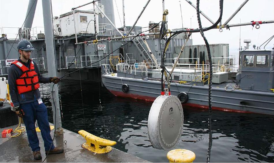
Figure 5. The Geospectrum, Inc. low frequency source (LFS) (f₀ = 32 Hz, Δf = 10 Hz, 1 m diameter, 0.2 m thick, 270 kg). (Figure provided by Geospectrum, used with permission).

Acoustic receiver technology has also improved. Sub-basin-scale ocean acoustic tomography experiments have taken advantage of the flexibility of autonomous, moored systems. The expected magnitude of travel-time perturbations associated with the ocean mesoscale is roughly 100 ms. The differential travel-time signal from reciprocal transmissions is an order of magnitude smaller. The requirements to keep time with millisecond accuracy in submerged instruments for a period of a year or more, measure the motion of the moored sources and receivers to within a meter or so in order to correct for travel-time perturbations due to changes in range, and record the large amounts of data generated by the acoustic receptions made for early instruments that were sufficiently complex to be accessible only to highly specialized research groups [Munk et al. (1995) provides a detailed discussion of the observational methods used in acoustic tomography]. Modern developments in data acquisition systems and data storage have now made the required instrumentation much more user-friendly. For climate-oriented, basin-scale experiments with requirements for high power and long duration, however, cabled systems are preferred. (Hybrid systems are of course possible). Mooring motion and accurate timing are not problems in systems mounted on the seafloor and cable-connected to shore. The ATOC project relied on cabled systems, for example, augmented by a few autonomous vertical receiving arrays deployed for year-long periods to better characterize the propagation (ATOC Instrumentation Group, 1994).

The processing of tomographic data to obtain time series of travel times has become much more routine in recent years. For both moored and cabled systems, the signal processing and generation of time series of travel times for resolved acoustic ray paths has been labor intensive and subjective. After matched filtering and beamforming of the received signals, the procedure is to pick the peaks in the processed receptions. The peaks must then be associated with predicted ray arrivals. This procedure must be repeated for each reception for every source-receiver pair. However, internal-wave-induced scattering of the received signals impairs the ability to associate a measured peak with a computed ray path. Two procedures were developed to address these issues (Dzieciuch, 2014). First, an estimator-correlator that explicitly accounts for scattering is used to smooth the arrival pulse and improve the signal-to-noise ratio. Second, after defining an error metric that accounts for peak amplitude, travel time, and vertical arrival angle, the Viterbi algorithm has been successfully adapted to the task of automated peak tracking, eliminating the need to manually select appropriate peaks in each reception.

In the past, stochastic inverse methods have most commonly been used to interpret acoustic travel times to obtain ocean temperatures and currents (e.g., Munk et al., 1995). With recent improvements in the vertical resolution and realism of ocean circulation models, acoustic travel times are now being used to directly constrain the models, taking advantage of the models to combine acoustic (and other data) from different times and locations in a way that is consistent with ocean dynamics (e.g., Lebedev et al., 2003). Time-evolving ocean circulation models implicitly supply a large amount of information about the ocean by enforcing the conservation of mass, momentum, and other properties. The practice of combining data with models, referred to as state estimation or assimilation, simultaneously tests and constrains the models. A variety of approaches are available to solve this problem, e.g., variational data assimilation (4DVAR) and ensemble Kalman filtering (EnKF) (e.g., Munk et al., 1995; Gopalakrishnan et al., 2019).

Combining integral tomographic data with time-evolving models does not differ in any fundamental way from using other data types, but tomographic data do differ from most other oceanographic data because their path-integral sampling and information content tend to be localized in spectral space rather than in physical space. It is therefore important to use methods that preserve the integral information contained in the acoustic travel times. Approximate data assimilation methods optimized for measurements localized in physical space are generally inappropriate because they do not preserve the non-local tomographic information (Cornuelle and Worcester, 1996). The data types used to constrain the models are largely transparent to the user of the resulting ocean state estimates, placing the rather unfamiliar acoustic data on the same footing as more familiar data types.

Although state estimation employing general ocean circulation models in ice-free regions has received the most attention, state estimation employing coupled ocean-sea ice models has received increased attention in the past decade (Fenty and Heimbach, 2013; Stammer et al., 2016; Nguyen et al., 2017). Present ice-ocean coupled models can assimilate sea ice parameters from remote sensing and profiles from floats and drifting ice buoys. The sea ice forecasts are improved through the assimilation of sea ice parameters. However, there is a significant gap in under-ice observations to evaluate or constrain the ice-ocean models. The ice-ocean models are therefore unconstrained and their performance is more or less unknown. The effect of repeating assimilation only on the surface and keeping the ocean under the ice unconstrained with data is unknown. Acoustic methods can be used to provide data to test the large-scale behavior of the ocean-sea ice models and, eventually, to constrain them.

Underwater Acoustic Positioning and Navigation

Positioning, Navigation and Timing (PNT) are vital infrastructure services of our modern technical society. PNT needs to be extended throughout the subsea environment. PNT is a combination of three distinct, constituent capabilities:

1. Positioning is the ability to accurately and precisely determine one’s location referenced to a standard geodetic system;

2. Navigation is the ability to determine current and desired position (relative or absolute) and apply corrections to course, orientation, and speed to attain a desired position anywhere in the domain of concern; and

3. Timing is the ability to acquire and maintain accurate and precise time anywhere in the domain of interest within user-defined timeliness parameters; it also includes time transfer.

Navigation is real time and necessarily depends on positioning, and positioning depends on timing.

A key aspect of the multi-purpose concept is to transfer the precise measurement of travel time between a source and receiver, as done in tomography, to the long-range underwater positioning and navigation community as exemplified by RAFOS float positioning and AUV navigation. Providing an underwater navigation capability is particularly important in ice-covered regions, where floats, gliders, and AUVs have difficulty surfacing to obtain their positions. Multipurpose acoustic networks allow economy in source signaling: the same acoustic signals are used for both tomography and positioning. The Global Navigation Satellite System (GNSS), of which the US Global Positioning System (GPS) is part, has enabled ionospheric (electron density) and atmospheric (temperature, precipitable water vapor) tomography, while providing its core PNT service. The relatively expensive satellites provide signals to 10–100s of low earth orbiting satellites (radio occultation) and 1000s of ground stations to obtain dense, global coverage over land and ocean. For the ocean case, acoustic sources can transmit to both mobile vehicles and fixed receivers, solving for position and sound speed (temperature) in a joint estimation problem.

The difference between RAFOS and what has been called RAFOS-2 is comparable to the difference between old long-range navigation (LORAN) and Transit positioning and GPS today. The increased bandwidth of RAFOS-2/tomographic signals yields better positioning accuracy (Duda et al., 2006; Van Uffelen et al., 2016). Figure 6 shows simulated arrival patterns for a narrow band 1.6-Hz RAFOS signal, which is about 1 s in duration, equivalent to 1600 m position uncertainty, and for a RAFOS-2/tomography signal with a 50-Hz bandwidth, where individual arrival peaks are 20 ms wide, giving roughly 30 m range uncertainty (assuming 1500 m/s sound speed).

FIGURE 6

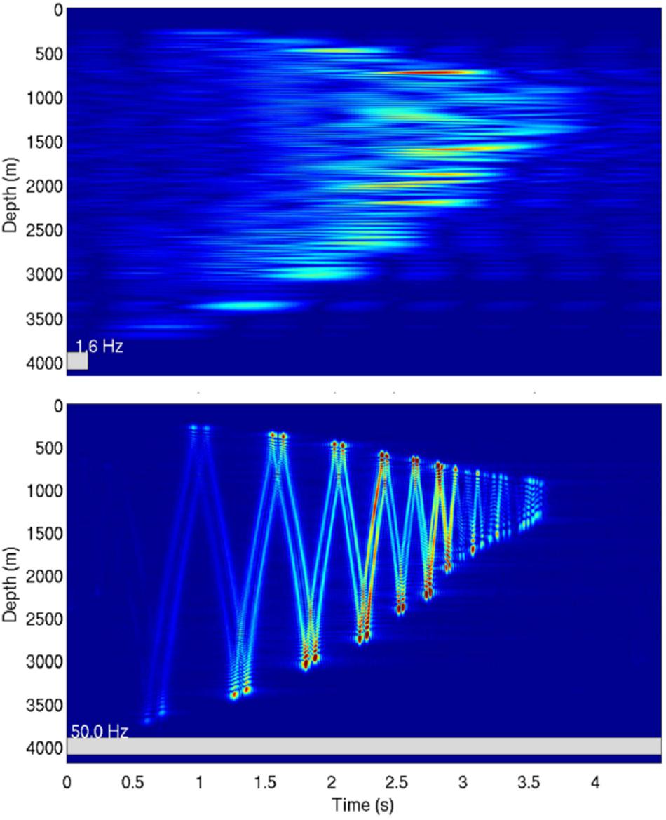
Figure 6. Arrival patterns for a 1145-km transmission path in the North Atlantic Ocean for systems with 80-s linear FM signals of 1.6-Hz (upper, RAFOS) and 50-Hz bandwidth (lower, RAFOS-2/tomography) and 260-Hz center frequency (source at 700 m depth, receiver at 2000 m depth). The time scale is reduced time, which removes the gross transmission delay between the source and receiver. Positioning uncertainty for the first case is (sound speed/bandwidth) ∼1000 m, while for the second it is 30 m (Duda et al., 2006, used with permission).

Precision glider positioning was in fact demonstrated in the 2010–2011 North Pacific Acoustic Laboratory (NPAL) Philippine Sea Experiment (PhiiSea10) (Van Uffelen et al., 2016). Six broadband, 250-Hz tomography sources were deployed in a pentagonal array 660 km in diameter. Four Seagliders, each equipped with an acoustic receiver and the ability to keep precise time (syncing to GPS time while the Seagliders were at the surface), recorded receptions. Subsequent analysis showed that estimated underwater position errors were reduced from 900 m RMS using standard glider positioning to about 80 m RMS when incorporating measured travel times, over 700 km ranges (Figure 7).

FIGURE 7

Figure 7. (Top) Acoustic Seaglider tracks in the Philippine Sea. Heavy dots indicate positions of gliders while collecting data. Squares indicate deployment positions. Black diamonds indicate positions of the acoustic transceiver moorings. A moored distributed vertical line array (DVLA) of hydrophone receivers was also deployed as part of the experiment. (Center) Circles indicate acoustically derived ranges from sources T1 (red, 275.6 km), T2 (orange, 115.4 km), T3 (green, 384.6 km), T4 (blue, 563.0 km), and T5 (magenta, 493.5 km) for SG513 Dive 204, Reception 1. Diamonds of the same colors indicate source positions. On this scale, the range circles appear to cross at the measured glider location. An expanded view of the region near the intersection of the circle arcs (bottom) shows the dead reckoning dynamically estimated positions for each source reception (stars corresponding in color with those listed above) and corresponding acoustically derived positions resulting from the least squares inversion (triangles). The black triangle indicates the corresponding position, which neglects the glider motion between transmissions (Van Uffelen et al., 2016, used with permission).

In ice-covered regions, work has been progressing along several lines. Using conventional narrow bandwidth RAFOS sources, Argo floats have been positioned (after the fact) to 400 km range (Klatt et al., 2007). Gliders have navigated under ice in Davis Strait (Webster et al., 2014) and Fram Strait (Sandven et al., 2011) with position uncertainties on the order of kilometers or more. More recently in the Arctic, higher frequency (900 Hz) instrumentation has been used in an integrated system with ice-tethered GPS synchronized navigation transceivers (i.e., the “satellites”) talking to gliders. As with GPS, low data rate source position information is transmitted to enable the gliders to perform absolute geo-positioning and navigation. Additional information can also be transmitted, in this case new surfacing target waypoints. This system has been tested; performance is a function of range, the particular acoustic conditions present and the vertical position of the glider relative to structure in the sound channel (Freitag et al., 2015; Webster et al., 2015; Lee et al., 2017). These examples show that no one solution fits all, but that significant progress is being made toward multipurpose acoustic systems; especially in the last case all the elements are there.

The incremental cost of using a broadband tomography source relative to a narrowband RAFOS source is small compared to mooring and ship time costs. This simultaneous improvement in positioning and associated navigation accuracy coupled with obtaining tomographic temperature is a major motivator for the multi-purpose concept. To obtain subsea positioning accuracy of 10 s of meters, one will need to account for the 4-D variation in sound-speed (e.g., mesoscale variability). For real-time subsea navigation this is clearly challenging; for delayed mode positioning, this would likely be done in the context of a large joint ocean-position estimation procedure.

Passive Acoustic Monitoring

Passive acoustic monitoring recording devices are now key to regional strategic plans for the successful monitoring of natural, anthropogenic, and animal sound. Audio data receivers support multiple hydrophones and associated recording channels and contain massive amounts of data storage, thanks to advances in non-volatile memory storage capacity and low-power digital signal processors. An autonomous directional PAM acoustic receiver array on a bottom lander is shown in Figure 8. Some acoustic recording systems contain sufficient on-board processing power to support real-time data reduction in the form of spectrogram generation, detection and classification of specific sounds, and localization of sounds from hydrophone arrays. For example, for ocean gliders equipped with acoustic receivers with on-board whale call classification software, only short data packets need be transmitted via Iridium satellite data connections to then allow real-time whale positions to be added to the automated identification system (AIS) used on ships and by vessel traffic services (Davis et al., 2016) to track vessel locations.

FIGURE 8

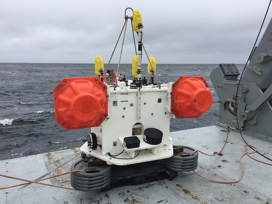
Figure 8. Atlantic Deepwater Ecosystem Observatory Network (https://adeon.unh.edu) acoustic lander. A tetrahedral hydrophone array comprising four M36 hydrophones within an Autonomous Multichannel Acoustic Recorder (AMAR; JASCO Applied Sciences) located under the yellow protection covers. Two sets of transducers are shown mounted on the bottom of the lander looking upwards as part of a 4-frequency Acoustic Zooplankton-Fish Profiler (AZFP, ASL Environmental Sciences) echosounder system for capturing water column backscatter. (Photo by J. Miksis-Olds, used with permission).

Passive acoustic monitoring receivers that are part of multipurpose acoustic observing systems need to have accurate and synchronized time bases. Timing is absolutely fundamental to undersea positioning, navigation and tomography, which use precision travel-time data, necessitating synchronized time bases across all platforms. Clock drift between acoustic sources and a receiver on an autonomous platform is the primary source of positioning uncertainty (Webster et al., 2015). Achieving synchronous time is straightforward for systems that have regular access to GPS signals. It is more difficult for autonomous subsea systems, but the technology to do so has been demonstrated, both via use of chip-scale atomic clocks and using time transfer methods, via acoustic communications.

Network Technology

One of the technologies that will be key to the vision of a multipurpose acoustic network as part of ocean observing systems is flexible low-power software-defined underwater signal processing systems. To support underwater sensor networks, next-generation Underwater Acoustic Networks (UANs) must be able to adapt their communication and networking protocols in real-time based on the environmental and application conditions. UAN developers initially found that commercially available acoustic modems, their embedded software systems being largely closed and proprietary, were not flexible enough to satisfy the requirements. This has led to a modular, evolving software-defined radio (SDR) framework for both research and commercial UAN devices supporting all layers of a network protocol stack, including the ability to flexibly encode/decode, in software, acoustic signal modulation at the physical layer (Dol et al., 2017). Such SDR technology enables, for example, an AUV to flexibly decode and process a multiplicity of source signal types: narrow-band RAFOS signals; wide-band frequency-modulated (FM) or phase-shift-keyed tomography/navigation (RAFOS-2) signals; or simple phase-shift keyed data packets. This allows a variety of acoustic source types to co-exist and evolve on multipurpose acoustic networks. Similarly, software algorithms for specific signal classification (e.g., commands, whale call identification, ship noise, estimates of rainfall, wind, or specific ice deformation events) can co-exist on board such an AUV or tomography SDR. Eventually, these decoded characteristics can be relayed to shore as compact metadata rather than voluminous raw acoustic data. An example of such SDR flexibility was demonstrated by the WHOI Micro-Modem 2 (Gallimore et al., 2010), deployed in 2014 on Seagliders in the marginal ice zone of the Chukchi Sea, which decoded RAFOS-like signals for travel-time estimates (linear FM sweep, 900-Hz center frequency, 25-Hz bandwidth, per above), as well as a phase-modulated signal that encoded a 72-bit data packet containing an ice-tethered (moving) acoustic source location (high resolution latitude and longitude) and a new target glider waypoint (low resolution latitude and longitude) (Freitag et al., 2015; Webster et al., 2015).

Acoustics Addressing Ocean Observing Needs

Discovery

Innovative tools that lead to new discoveries, which ultimately lead to hypothesis-driven science and finally sustained application, enable forward momentum in science. Because sound travels farther and faster than any other signal underwater, acoustics is the primary mode of probing the ocean volume, a form of remote sensing, whether it be fish navigating by the sound of surf or AUVs mapping the mid-ocean ridges, whales communicating and socializing, or measuring ocean basin heat content and currents.

Using the new tools to pick the “low-hanging fruit” catalyzes discovery. New tools or techniques in one field can be repurposed for ocean use, or a simple upgrade to an existing tool can make it much more versatile. Here we briefly explore the vision of what acoustics might bring to ocean observing on time scales of decades and longer, based on the technologies and networking described above.

There are direct analogies between acoustic underwater positioning and the global navigation system of systems (GNSS) that provide precise and accurate time and positioning. Our science and our society are now totally dependent on the latter and take it as an essential critical infrastructure service. We envision that multi-scale acoustic navigation systems will enable the same incredible development of applications that GNSS has created. It will be a major tool in helping us transition from a rather incoherent and chaotic view of the ocean, to a focused, evolving, coherent image. It will enable humankind (using mostly robotic avatars) to “see” the ocean volume.

With precise navigation one can envision using long-range/endurance AUVs to map the ocean floor (Woelfl et al., 2019). They will transit between a rather sparse network of cabled docking stations, which will also host the acoustic sources of the multipurpose system. There is no question that they will discover numerous volcanoes, hot and cold vent systems, mineral resources, and new life forms within these extreme environments. The latter is directly relevant to the conservation and sustainable use of marine biological diversity of areas beyond national jurisdiction (BBJN). With precise navigation, AUVs can fly over repeat paths to absolute locations with certainty to observe changes, enabling and servicing autonomous platforms, and serving as energy “tankers” and communications gateways. These platforms (as well as the AUVs) will be sampling a myriad of ocean and geophysical variables, including, for instance, heat and material fluxes from the seafloor (Deep Ocean Observing Strategy [DOOS], 2016, 2018; Levin et al., 2019).

Very importantly, such navigation is essential to sampling under ice in polar regions (Arctic and Antarctic), both for the physics as well as the ecosystems in such an extreme and ephemeral environment, e.g., massive springtime plankton blooms under Arctic sea ice that control the timing of water column primary production (Arrigo et al., 2012). While summer ice may disappear in the near future, ice during the rest of the year will likely persist for decades. Support for under-ice navigation would apply to AUVs as well as gliders and floats (ANCHOR Working Group, 2008; Mikhalevsky et al., 2015; Smith et al., 2019). In this case, not only would basic navigation be enabled, precise geolocation would allow results between the various disparate sampling platforms to be combined coherently within the framework of ocean data assimilation models (running the joint positioning/ocean state estimation). This applies equally to non-polar regions as well. High resolution in time and space tracking will open up a new domain of sampling space that includes smaller and faster ocean processes that are lost in crude RAFOS tracking (2 km, a few times per day).

We know there are sharp fronts in the ocean, but they are often difficult to sample. If they are sampled with mobile platforms, accurate georeferencing is important so that multiple sources of data can be coherently combined. Long-range acoustic propagation paths used in tomography are also sensitive to such features. One-second changes in travel time are observed as a result of Gulf Stream or Kuroshio meanders, for example (Spiesberger et al., 1983; Lebedev et al., 2003).

The use of “noise” sources of opportunity in a tomographic context is tantalizing, with sources being diffuse (wind, waves) to near points (ships, whales, earthquakes, glaciers). By cross-correlating noise signals received by spatially separated receivers, one can, in principle, infer acoustic arrival patterns for the intervening medium as if they were transceivers. This is well proven and utilized in seismology and many other fields. The critical factor in the ever-changing ocean, however, is the duration over which one can compute the cross-correlation before changes in the ocean medium cause the time delays between the receivers to vary (Kuperman, 2018). Some results have been obtained, for example using Antarctic ice noise as received on distant CTBTO arrays, and using vertical arrays listening to ships over short range. It may be that with the ever-increasing number of receivers being deployed with coherent signal processing, “passive tomography” will come to fruition (see Kuperman, 2018, for a recent review).

Extending this further, acoustic tagging of pelagic marine life is well underway (e.g., marine mammals, sharks) to address questions related to communication, foraging ecology, and impacts related to sound exposure (Johnson et al., 2009). With tags that include acoustic positioning capability, one can envision coherently processing the acoustic data in the context of other environmental data collected on other platforms (assuming the tag is eventually recovered). Information from animal tags have already been integrated into the Australian Ocean Data Network (AODN) (Hidas et al., 2018) and serve as a model for what is possible on a global scale.

Using acoustics to listen to marine life, from very small to very large, whether remotely or with a tag on an animal, will improve our understanding of communication and behavior. With accurate positioning, we can obtain finer and finer views of what the animals are doing, and why. With the improved ocean state estimates obtained by including acoustic tomography data, we will be able to more directly link animal behavior with ocean physics and determine how marine mammals function and adapt to the constantly changing conditions of a dynamic ocean.

Finally, the combined use of active and passive acoustics, as appropriate, to simultaneously observe the physics and biology will greatly aid the interpretation of the data. New insights will result when multi-frequency sonars and “acoustic vision” are coupled with observations of the physical flow throughout the water column, from the photic zone with the deep scattering layer, to the deepest hadal reaches.

Ecosystem Health and Biodiversity

Following closely on the heels of initial discovery is the quest to gain a full understanding of the environment surrounding targeted findings. The combination of active and passive acoustic technology is a powerful tool in building a comprehensive concept of ocean dynamics shaping the local or regional ecosystem. Ocean processes, marine life dynamics, and human ocean use are each inherently three-dimensional and time-dependent, and each occurs at many spatial and temporal scales. The versatility of acoustic observations provides the opportunity to obtain information over wide temporal and spatial scales. The value of ocean acoustic observations for understanding biology and ecosystems has been internationally recognized through the acceptance of the proposal by the International Quiet Ocean Experiment program to the GOOS Biology and Ecosystems Panel for the consideration of Ocean Sound as an Essential Ocean Variable (Miksis-Olds et al., 2018) and by the convening body of the Deep Ocean Observing Strategy (Deep Ocean Observing Strategy [DOOS], 2016, 2018). Additionally, the application of passive acoustic recordings in constructing underwater soundscapes to better understand ocean ecosystem dynamics has gained community traction. Clear evidence of the value and application of underwater soundscapes is demonstrated by the effort of the International Organization for Standardization (ISO) in developing ISO standard 18405 on Underwater Acoustics-Terminology to help ensure research measurements are repeatable and comparable across projects (International Organization for Standardization [IOS], 2017). ISO 18405 defines the underwater soundscape for the first time and illustrates the growing maturity of this ocean variable.

Ocean sound is a national and international focus because it crosses borders unimpeded. Acoustic signals, as opposed to visual and chemical signals, can propagate long distances in the ocean and provide a means for marine life and humans to gain information about the environment and for marine animals to exchange critical information. Passive acoustic technology allows us to eavesdrop on marine life interactions and physical processes that create the local soundscape. A soundscape is the characterization of the ambient sound in terms of its spatial, temporal and frequency attributes, and the types of sources contributing to the sound field (International Organization for Standardization [IOS], 2017). Passive acoustic recordings are used non-invasively to assess environmental sound levels, surface conditions, human activity, and the distribution and biodiversity of vocalizing marine life. Active acoustic technology provides a high-resolution (in both time and space) measure of biological (zooplankton and fish abundance and distribution) and physical oceanographic processes (internal waves, micro-turbulence, and frontal systems) through time series of acoustic backscatter measurements (Lavery et al., 2009).

A great deal of information related to ocean ecosystems can be gained simply by assessing the ambient sound. The concept of using information in ambient sound as cues to direct movement or identify appropriate habitats has recently been identified as a new field of study referred to as soundscape orientation, and the concept is also included within the broader field of soundscape ecology in the scientific literature (Slabbekoorn and Bouton, 2008; Pijanowski et al., 2011). A large number of aquatic species use sound cues contained in local soundscapes to navigate, forage, select habitat, detect predators, and communicate information related to critical life functions (e.g., migration, breeding, etc.). Consequently, marine animals ranging from the smallest larvae to the largest whales have evolved mechanisms for both producing and receiving acoustic signals. Information contained in underwater soundscapes provide a means to better understand the influence of environmental parameters on local acoustic processes (McWilliam and Hawkins, 2013; Miksis-Olds et al., 2013; Staaterman et al., 2014), assess habitat quality and health (Parks et al., 2014; Staaterman et al., 2014), and better understand the impacts and risks of human contributions to the soundscape on marine life.

Underwater soundscapes are dynamic, varying in space and time within and between habitats. Underwater soundscapes are highly influenced by local and regional conditions but, unlike most terrestrial soundscapes, distant sources are also significant contributors because sound propagates such great distances underwater. The underwater soundscape may be composed of contributions from human activity (e.g., shipping, seismic air gun surveys), natural abiotic processes (e.g., wind, rain, ice), non-acoustic biotic factors (e.g., animal movement), and acoustic contributions from sound producing, biological sources (e.g., marine mammals, fish, and crustaceans). The soundscape can be selectively decomposed and visualized to gain a greater understanding of the sources and environmental dynamics contributing to and shaping the temporal, spatial, and spectral patterns of the acoustic environment. In the early 1990s, the ATOC program began collecting ambient sound in order to begin to better understand soundscapes and answer such basic questions such as how often does the sound level exceed a certain value, and can the constituents of ambient sound be discriminated (Curtis et al., 1999). Figure 9 shows recent examples addressing these two questions.

FIGURE 9

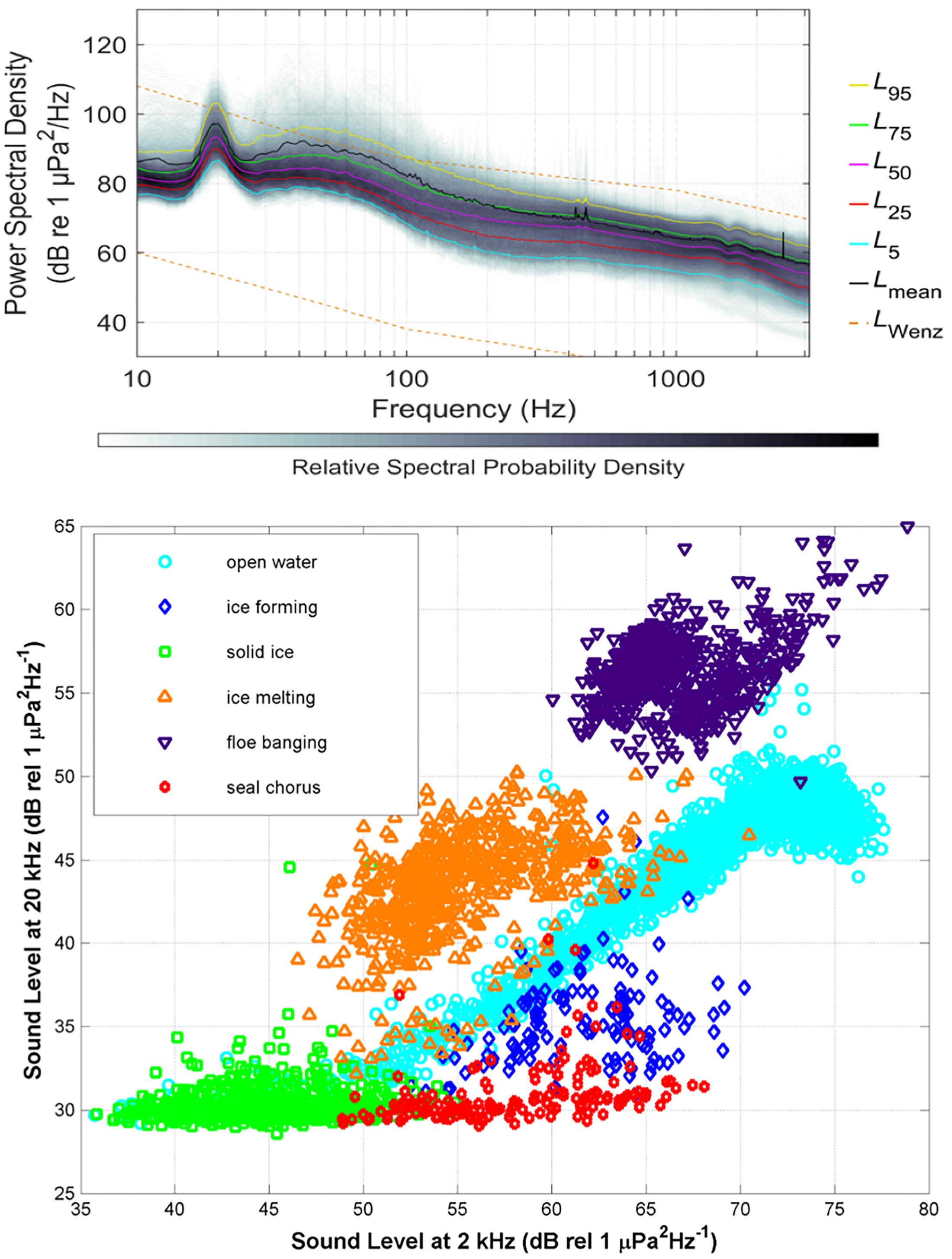
Figure 9. Two examples of how soundscape data is visualized. (Top) Summary of sound levels by an ADEON lander (Figure 8) along the Outer Continental Shelf east of Virginia based on 1-min, 1 Hz resolution analysis of data sampled at 375 kHz. Percentiles and relative spectral probability density for the 1 Hz spectra (Figure provided by Bruce Martin, JASCO Applied Science, used with permission). (Bottom) Soundscape recorded in the winter/spring of 2009 in the central region of the Bering Sea Shelf. Each point on the image represents the ratio of sound pressure level between 2 and 20 kHz at a specific point in time. The acoustic environment changed based on the presence of vocalizing ice seals and state of sea ice at the surface. Sources are color-coded based on their stereotyped source characteristics. [Figure was produced by Jeffrey Nystuen (APL-UW) and is a reproduction from Figure 5 in Van Opzeeland and Miksis-Olds, 2012, used with permission].

Indicators of habitat quality and biodiversity that were developed for terrestrial applications are now being applied to marine habitats and soundscapes (Denes et al., 2014; Parks et al., 2014; Staaterman et al., 2014). Acoustic analysis of a habitat’s soundscape using high level indicators such as the acoustic complexity index (ACI), acoustic entropy index, or acoustic similarity/dissimilarity indices provide a quantitative way to assess biodiversity and compare/contrast soundscapes of different habitats (Parks et al., 2014). Compared to in situ measurements of marine habitats by human divers, acoustic biodiversity indicators are less costly and less labor intensive. Acoustic systems also provide the added benefit of high temporal resolution resulting from long-term deployments of remote passive acoustic sensors. Acoustic diversity indicators are estimated by mathematically assessing the ratio of energy at different spectrum frequencies to make inferences about local community biodiversity. The larger the frequency bandwidth of recordings, the more information is available to accurately capture species and habitat diversity (Parks et al., 2014).

Successful examples of linking biodiversity and ocean sound come from studies on coral reefs and kelp beds. Healthy coral reefs and kelp habitats support high levels of biodiversity and produce an overall soundscape rich in temporal and spectral signatures created by the cacophony of vocalizing animals ranging from low-frequency fish calls to high-frequency, broadband sounds of snapping shrimp (Radford et al., 2008a; Staaterman et al., 2013). Kelp forests of New Zealand have shown diel, lunar, and seasonal trends in sound production with the most intense sounds occurring at dawn, dusk, and during the summer months when the abundance of sea urchins, snapping shrimp, and noise-emitting fish are highest (Radford et al., 2008b, 2010). In this system, there was good agreement between measures of acoustic and in situ diver collected biodiversity, illustrating the potential value of acoustic metrics for monitoring and assessing biodiversity of kelp habitats (Harris et al., 2016).

As powerful as passive acoustics can be in detecting, localizing, and providing information about local soundscape sources, passive acoustic technology fails when objects or phenomena are not producing sound. Active echosounder technology provides a time series of acoustic backscatter information that not only provides critical information on biology but also physical components of the water column (Lavery et al., 2009; Benoit-Bird and Lawson, 2016). The integration of multi-frequency echosounders in cabled and remotely deployed observation systems have contributed invaluable knowledge on marine life community structure, distribution and size of marine organisms, oceanic microstructure, and suspended sediments. By recording acoustic backscatter from at least two frequencies, the differences in backscatter between the two frequencies can be used to distinguish between different scatterers in the water column (Watkins and Brierley, 2002; Warren et al., 2003). Successful incorporation of upward looking, single beam echosounders in moorings at Ocean Station Papa (Trevorrow et al., 2005) and in the Bering Sea (Miksis-Olds et al., 2013; Miksis-Olds and Madden, 2014; Stauffer et al., 2015) demonstrate the maturity of this technology in providing time series of acoustic backscatter used to investigate the abundance and behavior of zooplankton and fish, predator-prey relationships, and community structure.

Successful use of multiple single-frequency echosounders to study ecosystem dynamics has led to the evolution of broadband systems (e.g., Lavery et al., 2010; Stanton et al., 2010; Benoit-Bird and Lawson, 2016), which are now being used in both cabled and moored configurations for inferring species composition. Broadband data have the advantage of improved spatial resolution, allowing better target isolation and noise suppression through the use of pulse compression techniques (Chu and Stanton, 1998; Ross et al., 2013). Broadband measurements and theoretical physics-based approaches for classifying zooplankton were successfully combined to classify biological scattering layers from the Victoria Experimental Network Under the Sea (VENUS) mooring in Saanich Inlet, British Columbia (Ross et al., 2013). Two years of broadband data (85–155 kHz) were collected from the VENUS system. Data processing classified scattering layers based on their assemblages into four animal groups: (1) diel migrating euphausiids; (2) chaetognaths; (3) fish; and (4) a mix of pteropods and bottom-to-oxycline migrating amphipods. Data generated from active acoustic systems provide biological information on trophic levels containing fish and zooplankton. When combined with the information obtained from passive acoustic systems related to physical conditions (e.g., surface conditions, ice cover, etc.), upper trophic level dynamics of marine mammals and other top predators, and even human use factors, underwater acoustics becomes a valuable tool in monitoring ecosystems in terms of overall function, biodiversity, and health.

Climate Variability and Change

Nearly four decades ago Munk and Wunsch (1982) proposed the establishment of a system for “Observing the ocean in the 1990s.” The hypothetical system that they described had two major observational components: ocean acoustic tomography and satellite measurements of sea surface topography (altimetry) and wind stress (scatterometry). (They also mentioned drifting floats but floats capable of profiling the upper 1000 m or so of the ocean did not exist at that time.) They expected that these complementary observations would “be assimilated into numerical modeling of the ocean circulation.” They listed the

“advantages and disadvantages of tomography as a tool for providing large-scale (and hence climatological) data…

Advantages

Large-scale spatial integration; information increases geometrically with the number of moorings; unattended recording over a year or more (1/3 year demonstrated so far); submerged instrumentation (of especial interest in regions of seasonal ice formation); remote sensing (of potential use in regions of strong currents); good vertical resolution.

Disadvantages

Sound speed is not a unique measure of temperature or density. However, in regions with stable temperature-salinity relations the separate temperature and salinity fields (and hence the density field) can be inferred to adequate precision…”

The notion of “unattended recording over a year or more” is now so routine that it seems quaint. Nonetheless, the basic advantages and disadvantages of the application of acoustic methods for studying climate variability are unchanged. The key advantage of measurements of climatological variability is that the spatial integration inherently provided by long-range acoustic transmissions suppresses the effects of mesoscale and smaller scale variability. The advantages of acoustic remote sensing for observing ocean climate variability were reiterated at the OceanObs’99 (Dushaw et al., 2001) and OceanObs’09 (Dushaw et al., 2010) conferences. These advantages still exist today. Obtaining the large-scale spatial averages needed for measuring climate change from profiles in which the majority of the variance is due to mesoscale and smaller scale variability is still very much a challenge. Satellite measurements of sea-surface properties, high-resolution vertical profiles of temperature and salinity (e.g., Argo), and large-scale average temperature and heat content from acoustic tomography are complementary for adequately sampling an ocean that varies on all time and space scales. As Munk and Wunsch (1982) noted, “A condition underlying any ocean observing system is that the ocean is transparent to sound, but opaque to electromagnetic radiation.”

What makes the case for the application of acoustic methods for measuring ocean climate variability more compelling now than in past decades? Munk and Wunsch (1982) were clearly ahead of their time. The first three-dimensional test of ocean acoustic tomography, the 1981 Tomography Demonstration Experiment, which lasted only 4 months, had just been completed (Behringer et al., 1982). The numerical ocean models available at the time (and in the 1990s, for that matter) did not have the vertical resolution needed for acoustic calculations. The situation is now dramatically different.

Long-Range Ocean Acoustic Thermometry

Transmissions over ranges of 1000 km or more have been used to measure large-scale ocean temperature and heat content, beginning with recording of the transmissions during the 1981 Tomography Demonstration Experiment in the Northwest Atlantic Ocean on bottom-mounted receivers at ranges of 1000–2000 km (Spiesberger et al., 1983). The application of long-range transmissions to measure temperature is often referred to as “acoustic thermometry,” usually in the context of transmissions for which there are few or no crossing acoustic paths. (Thermometry is a subset of acoustic tomography). Long-range measurements have also been made in the North Pacific Ocean, Mediterranean Sea, and Arctic Ocean. Transmissions over global scales were made during the 1991 Heard Island Feasibility Test (HIFT), but these very long ranges are not optimal from the perspective of measuring climate variability because the transmissions average across distinct climatic provinces (Munk et al., 1994).

Acoustic transmissions from sources located near the sound-channel axis to vertical receiving arrays over gyre scales (1000 km) (Worcester et al., 1994) and basin scales (3250 km) (Worcester et al., 1999) established conclusively that acoustic methods can measure range- and depth-averaged temperatures at gyre- and basin-scale ranges with a precision of a few millidegrees C (Figure 10). The early portions of the acoustic arrival patterns at long ranges consist of ray-like wave fronts that are resolvable, identifiable, and stable. The later parts of the arrival patterns (finale) do not contain identifiable ray-like arrivals due to scattering from internal-wave-induced sound-speed fluctuations. Nonetheless, the time at which the near-axial acoustic reception ends can be used as a surrogate for the group delay of the lowest acoustic normal mode, providing information on near-axial temperatures. These experiments were unique in combining long vertical receiving arrays, extensive concurrent environmental measurements, and broadband signals designed to measure acoustic travel times with millisecond precision.

FIGURE 10

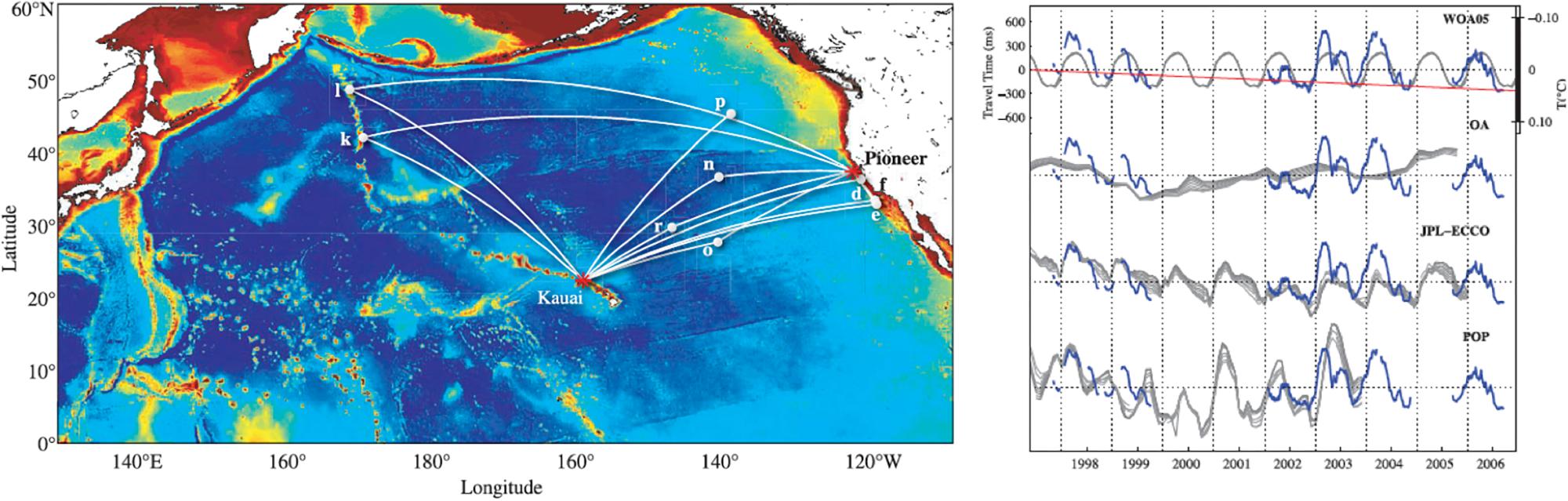
Figure 10. (Left) Acoustic propagation paths from the Kauai and Pioneer Seamount sources to receivers in the Pacific for the Acoustic Thermometry of Ocean Climate (ATOC) program. (Right) Comparison of travel times (blue) for acoustic paths with ocean climate models (gray). Jet Propulsion Laboratory “Estimating the Circulation and Climate of the Ocean” (JPL-ECCO) = ocean circulation model + data assimilation; OA, objective analysis; POP, Parallel Ocean Program model; WOA05, World Ocean Atlas 2005 (Dushaw et al., 2009, used with permission).

Although these results were favorable, at the time it was not understood how the early time fronts could be stable in the presence of internal-wave-induced scattering of the acoustic signals. In the (non-linear) geometric optics approximation, rays were expected to become chaotic at long ranges. Subsequent analyses showed that scattering tends to occur along wave fronts, rather than across them, giving resolvable, stable wave fronts (Godin, 2007). Further, wave-theoretic modeling, using normal mode and parabolic equation methods, has been applied to obtain travel-time sensitivity kernels (TSKs) without making the geometric optics approximation describing how travel times are affected by localized sound-speed perturbations anywhere in the medium (Skarsoulis and Cornuelle, 2004). Investigations of the structure and stability of the TSK in the presence of small-scale oceanographic variability that scatters acoustic signals show that ray-based travel-time inversions are valid even in this case (Dzieciuch et al., 2013). There is now a firm theoretical basis for the application of ray inversion methods.

Long-Range Transmissions and Ocean Models

Early attempts to use gyre- and basin-scale travel times to constrain ocean models were made by Menemenlis et al. (1997) and the Acoustic Thermometry of Ocean Climate (ATOC) Consortium (1998). At the time, primitive equation ocean general circulation models (OGCMs) did not have the vertical resolution needed to characterize ocean acoustic propagation and permit the accurate calculation of travel times. Statistical inverse methods were therefore used to convert the travel times to range-averaged ocean temperatures, which were then used as data to constrain primitive equation models.

The ATOC project continued over the decade 1996–2006, using sources installed off central California (1996–1999) and north of Kauai (1997–1999, 2002–2006) that transmitted to bottom-mounted and moored receivers in the North Pacific. These measurements were subsequently used to test more modern OGCMs (Dushaw et al., 2009, 2013). When attempting to compare the travel-time variability observed at bottom-mounted receivers for the duration of the ATOC project with model estimates, Dushaw et al. (2009) found that calculations based on the climatology in the World Ocean Atlas 2005 (WOA05) were able to reproduce the observed acoustic arrival patterns. The OGCM estimates available at the time proved incapable of doing so, however. The critical parameter for acoustic propagation calculations is the vertical sound-speed gradient, which was sufficiently unrealistic in the OGCM estimates to make the acoustic calculations fail. In order to proceed, the time means of the model temperature and salinity fields were removed and replaced with the annual mean fields from WOA05, making the assumption that the variability in the model estimates was realistic even though the mean fields were not. The differences between the observed travel time variability and that calculated from the models were sometimes substantial. Dushaw et al. (2013) subsequently used receptions on three vertical hydrophone arrays that were installed for about a year each in 1996 and 1998 to test the time-mean properties of the OGCM estimates. The observed acoustic arrival patterns were found to be in relatively good agreement with those computed for state estimates made by the Estimating the Circulation and Climate of the Ocean, Phase II (ECCO2) project, indicating that the numerical ocean models had reached a level of maturity by the time of Dushaw et al. (2013) such that the acoustic data could be used to provide useful additional constraints for ocean state estimation.

Ice-Covered Seas

The case for using acoustic methods to study climate variability is especially compelling in ice-covered regions, where long-term, large-scale, continuous observations of the ocean interior are difficult to obtain using other approaches. Most attention to date has focused on the rapidly changing Arctic (e.g., Jeffries et al., 2013), but acoustic methods are equally applicable in the seasonally ice-covered Southern Ocean around Antarctica.

Satellite images show a large reduction of sea ice in the Arctic (e.g., Meier et al., 2014). The satellites cannot observe the interior of the ocean underneath the sea ice, and less is therefore known about what is occurring in the ocean under the ice. Just below the sea ice there is a cold, fresh water layer that protects the ice from the warmer, saltier waters deeper in the ocean. Point measurements in some areas of the Arctic indicate that this layer is disappearing (Lique, 2015; Polyakov et al., 2017). This change can accelerate the melting of the sea ice. Additionally, it is not known how much heat is stored in the water masses under the protective water layer.

Previous basin-scale acoustic measurements made in the 1990s showed that the Atlantic Intermediate Water (Atlantic Layer) was warming. During the 1994 Transarctic Acoustic Propagation (TAP) experiment, ultralow-frequency (19.6 Hz) acoustic transmissions propagated across the entire Arctic basin from a source located north of Svalbard to a receiving array located in the Beaufort Sea at a range of about 2630 km (Mikhalevsky and Gavrilov, 2001). Modal travel-time measurements yielded the surprising result that the Atlantic Layer was about 0.4°C warmer than expected from historical data. Acoustic data collected on a similar path during April 1999 as part of the Acoustic Climate Observations Using Underwater Sound (ACOUS) project indicated further warming of about 0.5°C. These results were subsequently confirmed by direct measurements made from icebreakers and submarines (Mikhalevsky and Gavrilov, 2001).

Mikhalevsky et al. (2015) advocated the application of multipurpose acoustic networks in an integrated Arctic observing system (Figure 11). Several year-long experiments in Fram Strait (Sagen et al., 2016, 2017) and the Canada Basin have demonstrated the technology at a regional scale. It is now 20 years since the TAP and ACOUS measurements were made. The Coordinated Arctic Acoustic Thermometry Experiment (CAATEX), jointly funded by the United States, Norway, and Canada, will repeat these basin-scale measurements during 2019–2020. In addition to acoustic remote sensing (tomography), an integrated acoustic system would provide passive monitoring of ambient sound (ice, seismic, biologic, and anthropogenic) and under-ice navigation for drifting floats, gliders, and AUVs. Given the rapid rate at which the Arctic is changing, implementation of a sustained integrated observing system is urgent.

FIGURE 11

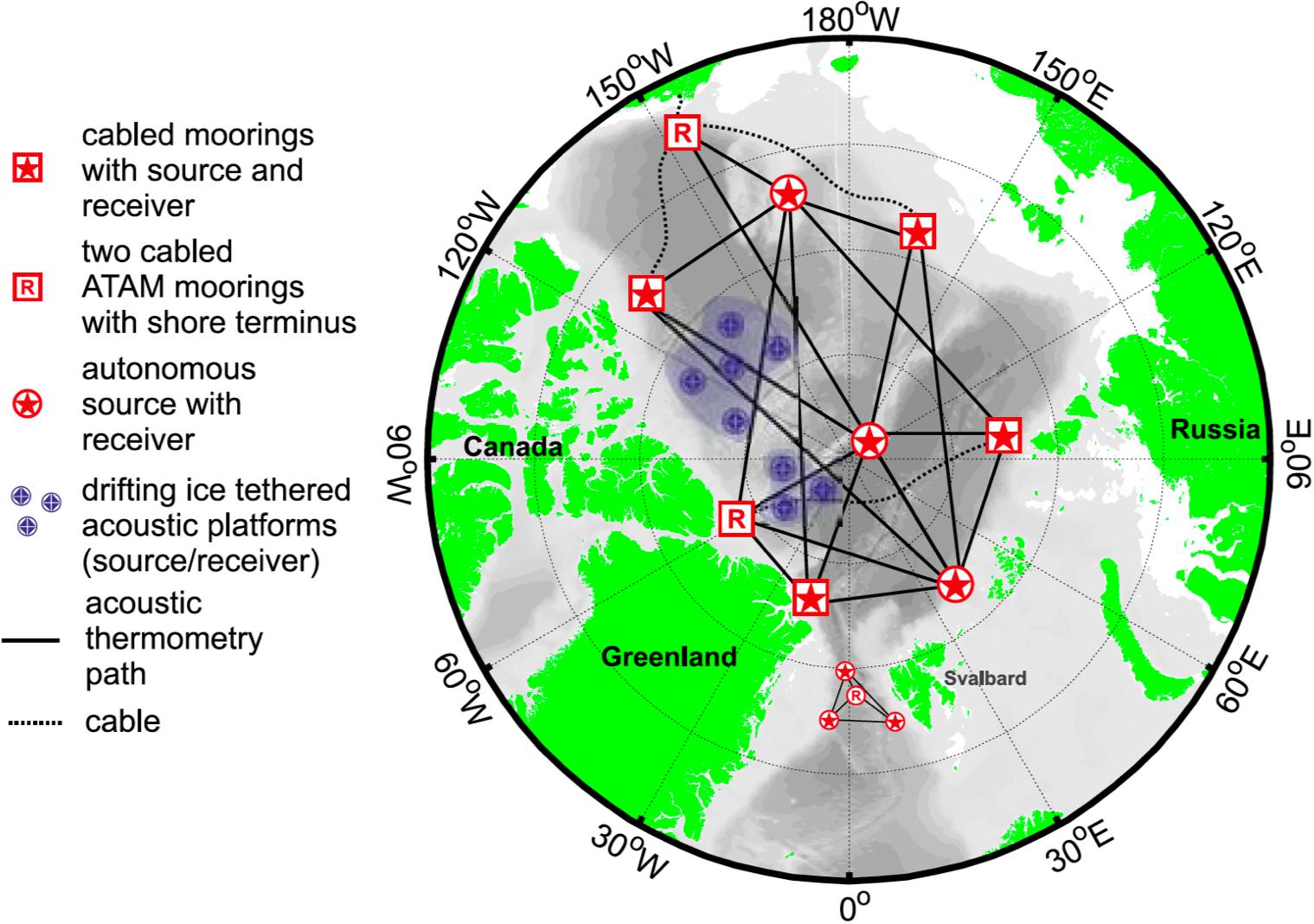
Figure 11. The notional basin-wide Arctic mooring network for acoustic tomography, oceanography, and underwater “GPS” system for navigation of and low rate communications with floats, gliders, and UUVs. The Acoustic Thermometry and Multipurpose Mooring (ATAM) applies to all the moorings shown (Mikhalevsky et al., 2015, used with permission).

Straits and Climate Choke Points

Geographically constrained regions of the ocean function as gateways for important exchanges of heat, salt, nutrients, and marine life itself, with implications for climate change and variability. For example, water mass exchanges between the Arctic Ocean and the Atlantic and Pacific Oceans occur through the Fram Strait, Bering Strait, Davis Strait, and the Canadian Archipelago. Long-term acoustic tomography measurements can help determine heat and salt fluxes through these straits, taking advantage of the integrating property of acoustic data.

For example, models show a series of complex interactions within Baffin Bay in which melting Greenland ice sheets lead to decreased southward transport of cold Arctic water via the Canadian Archipelago and increased northward transport of fresh Atlantic water via Davis Strait due to a strengthening of the gyre circulation in Baffin Bay. A positive feedback cycle develops as warmer water enters Greenland fjords, further enhancing the melting of marine-terminating glaciers (de la Guardia et al., 2015). Clearly, monitoring the long-term changes in heat content, salinity, and mean circulation are paramount to evaluating the importance of this feedback cycle.

In another example, Pacific Waters (PW) represent one-third of all Arctic freshwater and supply and 10–20% of the oceanic heat to the Arctic Ocean. The large Arctic sea-ice retreat of 2007 was likely caused by extreme oceanic flux of PW. Remotely sensed sea surface temperature (SST) is insufficient for quantifying the variability in estimating the heat content in the Bering Strait region (Woodgate et al., 2012), which suggests an opportunity for temperature estimates from measurements of acoustic travel time to contribute to estimates of heat content in that region.

A study in Fram Strait showed that while point measurements from moorings and integrated measurements from acoustic tomography lead to similar uncertainties in sound speed (from which salt water properties are retrieved), objective estimates using combined mooring and tomographic measurement lead to a threefold reduction in uncertainties. Further, unlike a 2-D mooring array, adding tomographic measurements offers the opportunity to capture the 3-D variability necessary to fully understand transports through Fram Strait (Dushaw and Sagen, 2016).

Tomographic measurements have been made in other Straits as well, in locations of climatic importance. For 3 months in 1996, 2 kHz transceivers were deployed in the Strait of Gibraltar. Reciprocal travel-time measurements diagonally across the Strait performed best for determining path-averaged velocity, while sum travel times provided good temperature measurements (Send et al., 2002). For the last decade, investigators led by A. Kaneko conducted many measurements in coastal seas. Most recently, the focus has been on measuring in the straits associated with the Indonesian Through Flow (ITF). Measurements in the Bali Strait resolved a five-layer vertical structure of flow as well as strong non-linear tides (Syamsudin et al., 2017). Future plans are to sustain these measurements and extend them to the Lombok and other straits. In this application, the remote sensing capability of the acoustics comes into play as nearshore (e.g., pier-mounted) equipment has a much higher probability of surviving than do instruments in the strait itself.

Hazards and Maritime Safety

The Comprehensive Nuclear-Test Ban Treaty Organization (CTBTO) is supporting the scientific use of International Monitoring System (IMS) data for disaster warning, marine hazard prevention and overall promotion of human welfare. The IMS functions as a Global Alarm System designed to detect not only nuclear explosions but also earthquakes able to produce tsunamis (CTBTO website: Disaster Warning and Science¹).

The verification regime of the Comprehensive Nuclear-Test-Ban Treaty (CTBT) regime relies on the IMS, which consists of 337 facilities worldwide and provides global coverage for signs of nuclear explosions. Of the 337 facilities, 11 are hydroacoustic stations responsible for covering the oceans. The hydroacoustic stations include five T-stations, which use on-shore seismometers to detect waterborne signals coupled into the Earth’s crust, and six cabled hydrophone stations with two triplets of moored hydrophones in a horizontal triangular configuration with a separation of 2 km (with the exception of one station in Australia which has a single triplet). At present, 100 IMS stations, both hydroacoustic and seismic, provide near real-time data to tsunami warning centers in 14 countries to enhance their capability to issue timely and precise warnings (Figure 12).

FIGURE 12

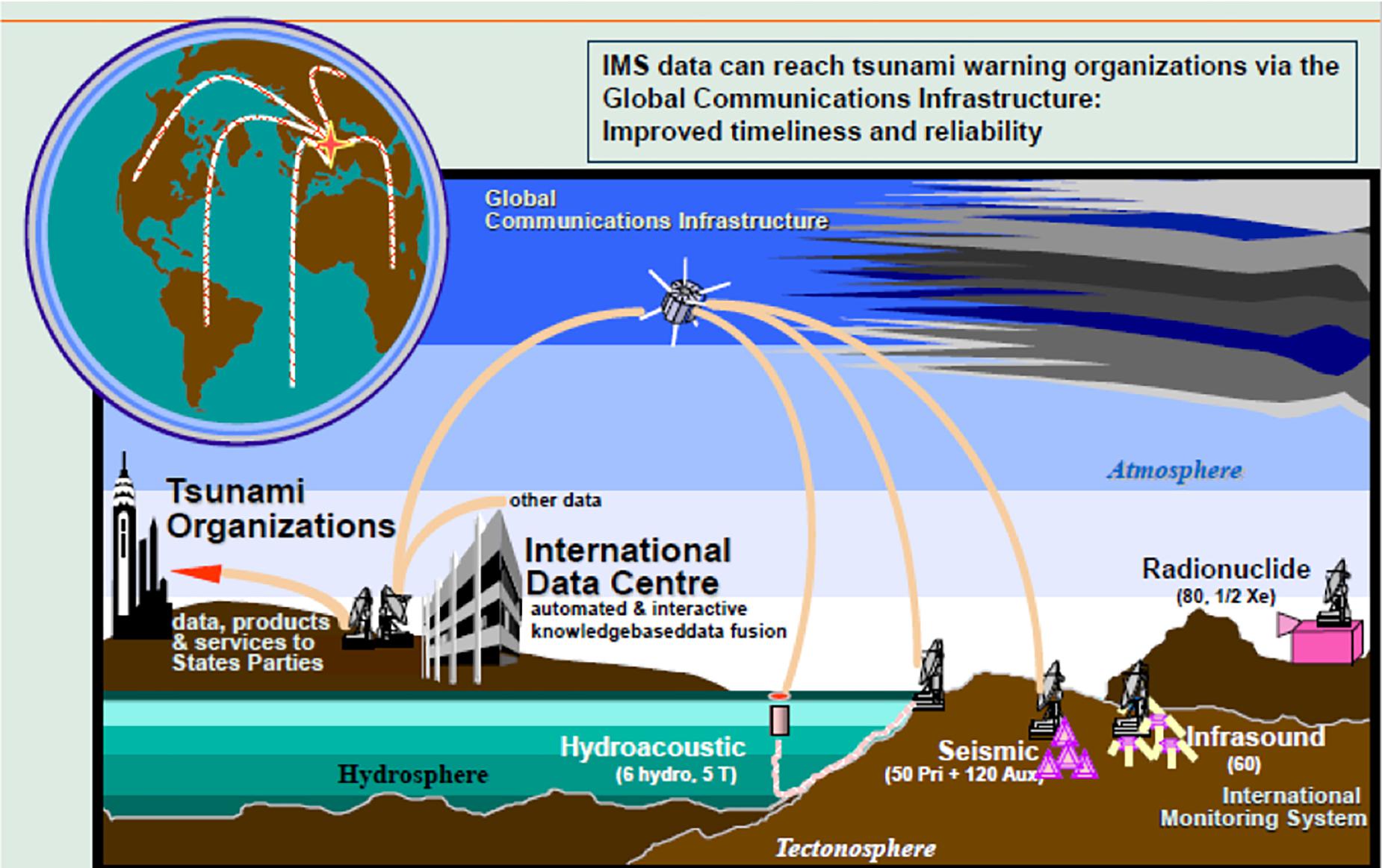
Figure 12. Data flow within the CTBTO IMS, with appropriate data and products forwarding to tsunami warning centers in real time (Figure provided by G. Haralabus, used with permission).

Hydroacoustic station warnings of underwater volcanic eruptions or undersea earthquakes could bring significant benefits to maritime traffic. For example, during the Tōhoku earthquake and the subsequently induced tsunami that struck Japan on 11 March 2011, the HA11 Wake Island (United States) hydrophone station helped track the wave as it propagated across the Pacific Ocean. Another example of the multitude of natural signals recorded at the IMS hydroacoustic stations is the magnitude 8.2 earthquake that occurred on 1 April 2014 in Northern Chile and was recorded at the HA03 Juan Fernandez (Chile) hydrophone station (Figure 13).

FIGURE 13

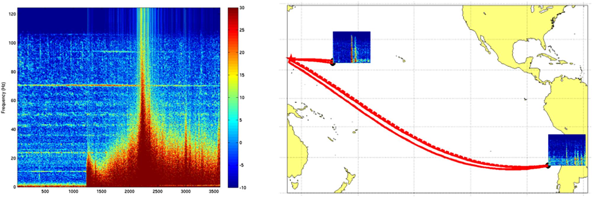
Figure 13. (Left) Frequency content of the 1 April 2014 northern Chile earthquake signal on an HA03 hydrophone (Juan Fernandez, Chile) versus time (in seconds) on the horizontal axis. The color scale is in decibels (dB), with red denoting higher energy content. Early arrivals are attributed to seismic waves traveling through the ocean crust and leaking acoustic energy into the water, however, most of the acoustic energy arrived later in the form of T-phase propagation in the SOFAR. (Right) Hydrophone recordings at HA11 (Wake Island, United States) and HA03 (15,000 km away) pertaining to bursting underwater gas bubbles emitted by an undersea volcano near the Mariana Islands (Figure provided by G. Haralabus, used with permission).

One of the greatest advantages offered by hydroacoustic stations is that they cover exceptionally large areas, compared to other technologies, due to the efficient way sound propagates in the water (Figure 3). In April 2014, underwater explosion-like signals emitted by an undersea volcano near the Mariana Islands in the North Pacific Ocean were received at HA03, more than 15,000 km away (Figure 13).

Hydroacoustic data from the IMS network provided assistance in the search for the missing Argentine submarine ARA San Juan (S-42). On 15 November 2017, two CTBTO hydroacoustic stations, namely HA10 (Ascension Island) and HA04 (Crozet), detected an unusual signal in the vicinity of the last known position of the submarine. The signal had the characteristics of an underwater impulsive event and occurred at 13:51 GMT on 15 November. Details and data were made available to the Argentinian authorities to support the ongoing search operations. The mutually beneficial collaboration between Argentinian researchers and hydroacoustic experts at CTBTO continues with further analysis of this unusual acoustic event (CTBTO, 2017a,b).

Passive acoustic monitoring is also currently being applied at a local and regional level to alert the shipping industry to the presence of hazards in the form of large whales. Off the east coast of the US, the endangered North Atlantic right whale migrates up and down the coast annually. Their surface behavior related to foraging puts them at high risk for ship collisions (Parks et al., 2014), which is costly to both the animal and the ship. The Right Whale Listening Network² implements a smart acoustic buoy system to continually listen for whale calls. If a right whale call is detected any time in the last 24 h, it is reflected on the website, and this information is also broadcast to mariners to reduce vessel speeds below 10 knots in an effort to reduce ship strikes. This technology has expanded in the form of a Whale Alert app³, which aims to reduce lethal whale ship strikes worldwide and across all large whale species.

Discussion

The implementation of a global multipurpose acoustic ocean observing system is beginning. The establishment of ocean sound as an Essential Ocean Variable is an important milestone in this process. Ocean sound is uniquely suited to observing ocean ecology and biology, both in passive and active forms. The infrastructure for positioning, navigation, timing (PNT) and communication, which is so critical to effective operations of all observing platforms in the ocean, directly leads to tomographic observations. With these active and passive components, the multipurpose system can be realized.

The elements to accomplish this have sufficient technical readiness and feasibility to implement the system. Passive receivers, often with arrays, are now commonplace; accurate timing and geo-referencing are required for them to be coherent elements of the larger system. Active sources suited to long-range acoustic propagation necessary for PNT and tomography are now off-the-shelf. Similarly, autonomous echosounder systems for short-range monitoring of water column biology are now commercially available. Acoustic signal processing is up-to-the-task, though the “big data” aspects are already somewhat daunting. The assimilation of tomographic travel time data into ocean models is understood but needs to be made routine with sustained data streams from operational systems. The same applies to acoustically determined high-resolution float and vehicle tracks; this needs to be done as a joint estimation problem.

A large proportion of PAM research programs and applications focus on questions pertaining to coastal waters due to the relatively easy access compared to outer continental shelves, concentration of human activities along the coasts, and regulatory/management concerns under national, regional, and local jurisdictions. PAM networks, like the CTBTO, demonstrate the value of global coverage, but have historically been limited to low frequency recordings due to constraints in power, sensor data storage capacity, required post-processing resources, and data management services. As discussed in this work, many of these obstacles have been overcome or are presently being addressed through advances in technology or repurposing methodologies from other fields. Consequently, PAM is a mature tool for ocean monitoring that is expanding in bandwidth, geographical scope, and application.

Future innovation related to PAM technology and applications is likely to come in the form of combining PAM with other non-acoustic sensing methods. For example, over the past 2–3 years, environmental DNA (eDNA) techniques, which have been used more in freshwater ecosystems, are now being explored in marine environments (Andruszkiewicz et al., 2017; Bakker et al., 2017; Gargan et al., 2017). The eDNA from targeted marine mammal species is detectable and comparable to both visual and acoustic surveys 2 h after an animal has swum through a volume of water (Baker et al., 2018). As eDNA technology and methodologies continue to develop in association with marine ecosystems, it is possible to envision an ocean observation system systematically addressing questions of ecosystem connectivity from estuarine habitats to deep ocean environments far offshore (Levin et al., 2019). Combining PAM with eDNA or genomic sensing is only one of the non-acoustic techniques that hold future promise in enhancing our ability to autonomously observe the ocean, and the likelihood of future generations developing completely new methods that are presently inconceivable is high.

To be used effectively, multipurpose acoustic observing systems should be deployed where they can uniquely make the largest contributions, filling gaps in the present observing system. Polar regions, near and under the ice in the Arctic and Antarctic are in desperate need of observations and sustained monitoring that only acoustics can provide. Such systems would simultaneously observe the changing heat content and effects on melting ice using tomography while at the same time providing positioning and navigation capability for under-ice floats and vehicles. It is especially important that broadband acoustic sources be used in conjunction with accurate clocks.

At the same time, the multitude of widely distributed PAM receivers in non-polar regions (e.g., CTBTO) can motivate multipurpose systems on global scale, perhaps with a longer time constant to implement. Judiciously locating cabled sources and using sources deployed from GO-SHIP vessels (providing sustained repeat hydrographic sections on decadal repeat timescales) can quickly provide wide-scale coherent tomographic coverage and derived heat content estimates, supplementing and complementing other, often incoherently sampled, observing elements. SMART telecommunication cables with integrated sensors will play a role as well (Howe et al., 2019).

Observing the ocean acoustically creates strong synergies with other observing programs, as reflected in the white papers in this Special Issue for OceanObs’19. Closing the sea-level budget (Leuliette, 2015; WCRP Global Sea Level Budget Group, 2018) requires accurate knowledge of ocean bathymetry (Woelfl et al., 2019), ocean sea level (Ponte et al., 2019), barystatic changes (mass of freshwater added or removed; Palmer et al., 2019), and thermostatic changes (e.g., changes in heat content; Meyssignac et al., 2019). Multipurpose acoustic observing systems will contribute to improved monitoring of volume, freshwater, and long-term heat fluxes, as well as monitoring long-term heat content changes at basin-scale, as well as in specific regions of global importance (e.g., Indonesian throughflow; Ravichandran, 2011; Sprintall et al., 2019). Multipurpose acoustic systems can provide ground-truth for ecosystem modeling and forecasting. Acoustic in situ rainfall and wind speed estimates can improve our observations of air-sea fluxes (Centurioni et al., 2019), particularly in sparely sampled regions such as the Southern Ocean (Swart et al., 2019) and polar regions (Smith et al., 2019) as well as improve our ability to monitor wind/current/wave interactions (Villas Bôas et al., 2019). The direct estimates of ocean state variables from acoustic tomography and acoustically located and navigated autonomous platforms operating in undersampled high-latitude regions will improve ocean state estimation (Heimbach et al., 2019). The rich applications of hydroacoustic monitoring from the CTBTO IMS demonstrate that additional observations from fixed acoustic transceiver nodes, coupled with soundscape maps provided by PAM, are important components of Eulerian observational systems, including tsunami warning (Angove et al., 2019).

Summary and Recommendations

We have outlined the current status of multi-purpose acoustic systems, noted the contributions they are making now and can make in the future, and discussed what gaps they can fill in the current ocean observing system. Based on this, we suggest that the following recommendations be included in the outcomes from the OceanObs19 conference.

Recommendation 1: OceanObs’19 recognizes the utility, both in terms of observing system capability as well as reduced effort and cost, of multipurpose acoustic observing systems, and recommends implementation in GOOS.

Recommendation 2: GOOS must develop a community capability to evaluate the present observing system and proposed additions thereto and apply the same to evaluating the benefits of precision acoustic navigation (of mobile platforms) and tomography. This could be accomplished by transitioning GODAE Ocean View to operational status as part of GOOS.

Recommendation 3: OceanObs’19 encourages implementation steps related to the ocean sound EOV, e.g., the incorporation of suitable acoustic receivers in general purpose instrument packages with necessary timing and geo-positioning capability and improved data access.

Recommendation 4: OceanObs’19 recognizes the extreme urgency of observing and monitoring the polar oceans, made difficult by ice cover, and recommends that multipurpose acoustic observing systems, along with other complementary systems including cabled ones, should be brought to operational status.

Dedication

This article is dedicated to Walter Munk, Oceanographer and Geophysicist, 1917–2019.

Author Contributions

BH led the effort and wrote the Introduction, Discovery, Discussion, and Summary. BH and ER wrote the Ocean Technology section. JM-O wrote the Ecosystem section. PW wrote the Climate Variability section. GH and JM-O wrote the Hazards and Maritime Safety section. All authors contributed to overall editing.

Funding

The authors were supported by their home institutions.

Conflict of Interest Statement

The authors declare that the research was conducted in the absence of any commercial or financial relationships that could be construed as a potential conflict of interest.

Acknowledgments

As part of the OceanObs’19 Conference white paper process, the Program Committee selected four related abstracts to combine into one for this Special Issue article:

Global Passive Monitoring of Sound to Understand Trends in Ocean Sound and Marine Life

Multipurpose Acoustic Networks in Ocean Observing Systems in Ice-Covered Regions

The Roles of Underwater Acoustics in Observing the Global Ocean

Baffin Bay Acoustic Navigation and Communication System: A Feasibility Study

This manuscript is the result. We gratefully acknowledge the contributions of the co-authors of these four abstracts, as well as others:

K. Atakan, W. Au, J. Ausubel, M. Babin, A. Beszczynska-Möller, O. Boebel, R. Brainard, S. Carr, B. Chakraborty, C. Clark, B. Cornuelle, C. de Jong, L. di Iorio, T. Duda, B. Dushaw, M. Dzieciuch, D. Fissel, L. Freitag, A. Gavrilov, P. Gorringe, C. Gourcuff, T. Hamre, K. Heaney, G. Heard, S. Jayne, B. Klein, M. Lammers, K. Latarius, D. Lecchini, C. Lee, H. Lin, R. McCauley, D. Menemenlis, P. Mikhalevsky, J. Miller, A. Mooney, S. Moore, A. Morozov, W. Munk, S. Nedelec, J. Orcutt, M. Parsons, C. Radford, S. Rintoul, S. Riser, M. Rixen, S. Sandven, S. Seeyave, S. Simpson, E. Skarsoulis, H. Søiland, M. Sørensen, B. Southall, K. Stafford, J. Stanley, R. Stephen, D. Tollefsen, J. Tougaard, P. Tyack, E. Urban, L. Van Uffelen, A. Vedenev, K. Vigness-Raposa, and C. Wunsch. We would like to thank CTBTO for its contribution and for promoting civil and scientific uses of data acquired by its international monitoring system. SOEST Contribution 10746.

Footnotes

1. ^https://www.ctbto.org/verification-regime/spin-offs-for-disaster-warning-and-science/
2. ^http://www.listenforwhales.org
3. ^www.whalealert.org

References

ANCHOR Working Group (2008). “Acoustic navigation and communications for high-latitude ocean research,” in Proceedings of the ANCHOR Workshop 2006 (Seattle, WA: University of Washington Applied Physics Laboratory).

Google Scholar

Andruszkiewicz, E. A., Starks, H. A., Chavez, F. P., Sassoubre, L. M., Block, B. A., and Boehm, A. B. (2017). Biomonitoring of marine vertebrates in monterey bay using eDNA metabarcoding. PLoS One 12:e0176343. doi: 10.1371/journal.pone.0176343

PubMed Abstract | CrossRef Full Text | Google Scholar

Angove, M., Arcas, D., Bailey, R., Carrasco P., Coetzee, D., Fry, B., et al. (2019). Ocean observations required to minimize uncertainty in global tsunami forecasts, warnings, and emergency response. Front. Mar. Sci. 6:350. doi: 10.3389/fmars.2019.00350

CrossRef Full Text | Google Scholar

Arrigo, K. R., Perovich, D. K., Pickart, R. S., Brown, Z. W., Van Dijken, G. L., Lowry, K. E., et al. (2012). Massive phytoplankton blooms under arctic sea ice. Science 336:1408. doi: 10.1126/science.1215065

PubMed Abstract | CrossRef Full Text | Google Scholar

Baker, C. S., Steel, D., Nieukirk, S., and Klinck, H. (2018). Environmental DNA (eDNA) from the wake of the whales: droplet digital PCR for detection and species identification. Fron. Mar. Sci. 5:133. doi: 10.3389/fmars.2018.00133

CrossRef Full Text | Google Scholar

Bakker, J., Wangensteen, O. S., Chapman, D. D., Boussarie, G., Buddo, D., Guttridge, T. L., et al. (2017). environmental DNA reveals tropical shark diversity in contrasting levels of anthropogenic impact. Sci. Rep. 7:16886. doi: 10.1038/s41598-017-17150-2

PubMed Abstract | CrossRef Full Text | Google Scholar

Behringer, D., Birdsall, T., Brown, M., Cornuelle, B., Heinmiller, R., Knox, R., et al. (1982). A demonstration of ocean acoustic tomography. Nature 299, 121–125. doi: 10.1038/299121a0

CrossRef Full Text | Google Scholar

Benoit-Bird, K. J., and Lawson, G. L. (2016). Ecological insights from pelagic habitats acquired using active acoustic techniques. Ann. Rev. Mar. Sci. 8, 463–490. doi: 10.1146/annurev-marine-122414-034001

PubMed Abstract | CrossRef Full Text | Google Scholar

Centurioni, L. R., Turton, J. D., Lumpkin, R., Braasch, L., Brassington, G., Chao, Y., et al. (2019). Global in-situ observations of essential climate and ocean variables at the air-sea interface. Front. Mar. Sci. 6:419. doi: 10.3389/fmars.2019.00419

CrossRef Full Text | Google Scholar

Chu, D., and Stanton, T. K. (1998). Application of pulse compression techniques to broadband acoustic scattering by live individual zooplankton. J. Acoust. Soc. Am. 104, 39–55. doi: 10.1121/1.424056

CrossRef Full Text | Google Scholar

Cornuelle, B. D., and Worcester, P. F. (1996). “Ocean acoustic tomography: integral data and ocean models,” in Modern Approaches to Data Assimilation in Ocean Modeling, ed. P. Malanotte-Rizzoli (Amsterdam: Elsevier Science BV), 97–115.

Google Scholar

Crease, J. (1962). Velocity measurements in the deep water of the western North Atlantic: summary. J. Geophys. Res. 67, 3173–3176. doi: 10.1029/JZ067i008p03173

CrossRef Full Text | Google Scholar

CTBTO (2017a). Available at: https://www.ctbto.org/press-centre/media-advisories/2017/media-advisory-ctbto-hydroacoustic-data-to-aid-in-search-for-missing-sub-san-juan/ (accessed November 23, 2017).

CTBTO (2017b). Available at: https://www.ctbto.org/press-centre/highlights/2017/ctbto-hydroacoustic-data-used-to-aid-search-for-missing-submarine-ara-san-juan/ (accessed November 24, 2017).

Curtis, K. R., Howe, B. M., and Mercer, J. A. (1999). Low frequency ambient sound in the north pacific: long time series observations. J. Acoust. Soc. Am. 106, 3189–3200. doi: 10.1121/1.428173

CrossRef Full Text | Google Scholar

Davis, R., Baumgartner, M., Comeau, A., Cunningham, D., Davies, K., Furlong, A., et al. (2016), “Tracking whales on the Scotian Shelf using passive acoustic monitoring on ocean gliders,” in Proceedings of the OCEANS 2016 MTS/IEEE (Monterey: IEEE), 1–4.

Google Scholar

de la Guardia, L. C., Hu, X., and Myers, P. G. (2015). Potential positive feedback between greenland ice sheet melt and Baffin Bay heat content on the west greenland shelf. Geophys. Res. Lett. 42, 4922–4930. doi: 10.1002/2015GL064626

CrossRef Full Text | Google Scholar

Denes, S. L., Miksis-Olds, J. L., Mellinger, D. K., and Nystuen, J. A. (2014). Assessing the cross-platform performance of marine mammal indicators between two collocated acoustic recorders. Ecol. Inform. 21, 74–80. doi: 10.1016/j.ecoinf.2013.10.005

CrossRef Full Text | Google Scholar

Dol, H. S., Casari, P., Van Der Zwan, T., and Otnes, R. (2017). Software-defined underwater acoustic modems: historical review and the NILUS approach. IEEE J. Oceanic Eng. 42, 722–737. doi: 10.1109/joe.2016.2598412

CrossRef Full Text | Google Scholar

Deep Ocean Observing Strategy [DOOS] (2016). DOOS 2016 Workshop Proceedings, Available at: http://www.deepoceanobserving.org/wp-content/uploads/2018/07/DOOS-2016-Workshop-Report-2017-04-13-V2.pdf (accessed July 11, 2019).

Deep Ocean Observing Strategy [DOOS] (2018). Science and Implementation Guide, Available at: http://www.deepoceanobserving.org/wp-content/uploads/2018/07/DOOS-SIG_CF_July2018_V2.pdf (accessed July 11, 2019).

Duda, T., Morrozov, A. K., Howe, B. M., Brown, M. G., et al. (2006). “Evaluation of a long-range joint acoustic navigation / thermometry system”, in Proceedings of the Oceans 2006 Conference (Boston, MA: IEEE).

Dushaw, B. D., and Sagen, H. (2016). A comparative study of moored/point and acoustic tomography/integral observations of sound speed in fram strait using objective mapping techniques. J. Atmos. Ocean. Technol. 33, 2079–2093. doi: 10.1175/jtech-d-15-0251.1

CrossRef Full Text | Google Scholar

Dushaw, B. D., Au, W. W. L., Beszczynska-Möller, A., Brainard, R. E., Cornuelle, B. D., Duda, T. F., et al. (2010). “A global ocean acoustic observing network,” in Proceedings of OceanObs’09: Sustained Ocean Observations and Information for Society, eds J. Hall, D. E. Harrison and D. Stammer, Vol. 2 (Venice: ESA Publication WPP-306). doi: 10.5270/OceanObs09.cwp.25

CrossRef Full Text | Google Scholar

Dushaw, B. D., Bold, G., Chiu, C.-S., Colosi, J. A., Cornuelle, B. D., Desaubies, Y., et al. (2001). “Observing the ocean in the 2000’s: a strategy for the role of acoustic tomography in ocean climate observation,” in Observing the Oceans in the 21st Century eds C. J. Koblinsky and N. R. Smith (Melbourne, VIC: Bureau of Meteorology), 391–418.

Dushaw, B. D., Worcester, P. F., Dzieciuch, M. A., and Menemenlis, D. (2013). On the time-mean state of ocean models and the properties of long-range acoustic propagation, J. Geophys. Res. Oceans 118, 4346–4362. doi: 10.1002/jgrc.20325

CrossRef Full Text | Google Scholar

Dushaw, B. D., Worcester, P. F., Munk, W. H., Spindel, R. C., Mercer, J. A., Howe, B. M., et al. (2009), A decade of acoustic thermometry in the North Pacific Ocean. J. Geophys. Res. Oceans 114, 1–24. doi: 10.1029/2008JC005124

CrossRef Full Text | Google Scholar

Dzieciuch, M. A. (2014). Signal processing and tracking of arrivals in ocean acoustic tomography. J. Acoust. Soc. Am. 136, 2512–2522. doi: 10.1121/1.4897404

PubMed Abstract | CrossRef Full Text | Google Scholar

Dzieciuch, M. A., Cornuelle, B. D., and Skarsoulis, E. K. (2013). Structure and stability of wave-theoretic kernels in the ocean. J. Acoust. Soc. Am. 134, 3318–3331. doi: 10.1121/1.4818846

PubMed Abstract | CrossRef Full Text

Fenty, I., and Heimbach, P. (2013). Coupled sea ice-ocean-state estimation in the labrador sea and baffin bay. J. Phys. Oceanogr. 43, 884–904. doi: 10.1175/JPO-D-12-065.1

CrossRef Full Text | Google Scholar

Freitag, L., Ball, K., Partan, J., Koski, P., and Singh, S. (2015). “Long range acoustic communications and navigation in the Arctic,” in Proceeding of the OCEANS 2015 - MTS/IEEE Washington (Washington, DC: IEEE).

Google Scholar

Gallimore, E., Partan, J., Vaughn, I., Singh, S., Shusta, J., and Freitag, L. (2010). “The WHOI micromodem-2: a scalable system for acoustic communications and networking,” in Proceeding of the Oceans 2010 MTS/IEE (Seattle, WA: IEEE).

Google Scholar

Gargan, L. M., Morato, T., Pham, C. K., Finarelli, J. A., Carlsson, J. E. L., and Carlsson, J. (2017). Development of a sensitive detection method to survey pelagic biodiversity using eDNA and quantitative PCR: a case study of devil ray at seamounts. Mar. Biol. 164:112. doi: 10.1007/s00227-017-3141-x

CrossRef Full Text | Google Scholar

Godin, O. A. (2007). Restless rays, steady wave fronts. J. Acoust. Soc. Am. 122, 3353–3363. doi: 10.1121/1.2799479

PubMed Abstract | CrossRef Full Text | Google Scholar

Gopalakrishnan, G., Hoteit, I., Cornuelle, B. D., and Rudnick, D. L. (2019). Comparison of 4DVAR and EnKF state estimates and forecasts in the Gulf of Mexico, Q. J. R. Meteorol. Soc.145, 1354–1376. doi: 10.1002/qj.3493

CrossRef Full Text

Haralabus, G., Zampolli, M., Grenard, P., Prior, M., and Pautet, L. (2017). “Underwater acoustics in nuclear-test-ban treaty monitoring”, in Applied Underwater Acoustics: Leif Bjørnø, eds T. Neighbors and D. Bradley (Chicago: Elsevier Science).

Harris, S. A., Shears, N. T., and Radford, C. A. (2016). Ecoacoustic indices as proxies for biodiversity on temperate reefs. Methods Ecol. Evol. 7, 713–724. doi: 10.1111/2041-210x.12527

CrossRef Full Text | Google Scholar

Heaney, K. D. (2015). “Advanced computation of three-dimensional long-range acoustic propagation for improved localisation methods,” in Proceedings of the International Hydroacoustics Workshop (Vienna: CTBTO).

Heimbach, P., Fukumori, I., Hill, C. N., Ponte, R. M., Stammer D., Wunsch, C., et al. (2019). Putting it all together: adding value to the global ocean and climate observing systems with complete self-consistent ocean state and parameter estimates. Front. Mar. Sci. 6:55. doi: 10.3389/fmars.2019.00055

CrossRef Full Text | Google Scholar

Hidas, M., Proctor, R., Mancini, S., Blain, P., Gordon, L., Scheibner, A., et al. (2018). “Automated data ingestion for the australian ocean data network,” in Proceedings of the 20th EGU General Assembly Conference Abstracts, Vienna.

Google Scholar

Howe, B. M., Arbic, B. K., Aucan, J., Barnes, C., Bayliff, N., Becker, N., et al. (2019). SMART cables for observing the global ocean: science and implementation. Front. Mar. Sci. 6424. doi: 10.3389/fmars.2019.00424

CrossRef Full Text | Google Scholar

Howe, B. M., and Miller, J. H. (2004). Acoustic sensing for ocean research. J. Mar. Tech. Soc. 38, 144–154. doi: 10.4031/002533204787522811

CrossRef Full Text | Google Scholar

International Organization for Standardization [IOS] (2017). Underwater acoustics—Terminology. ISO/DIS 18405.2:2017. Available at: https://www.iso.org/standard/62406.html (accessed July 11, 2019).

Jeffries, M. O., Overland, J. E., and Perovich, D. K. (2013), The Arctic shifts to a new normal. Phys. Today 66, 35–40. doi: 10.1063/PT.3.2147

CrossRef Full Text

Johnson, M., de Soto, N. A., and Madsen, P. T. (2009). Studying the behaviour and sensory ecology of marine mammals using acoustic recording tags: a review. Mar. Ecol. Prog. Ser. 395, 55–73. doi: 10.3354/meps08255

CrossRef Full Text | Google Scholar

Klatt, O., Boebel, O., and Fahrbach, E. (2007). A profiling float’s sense of ice. J. Atmos. Ocean. Technol. 24, 1301–1308. doi: 10.1175/JTECH2026.1

CrossRef Full Text | Google Scholar

Kuperman, W. A. (2018). Using noise to image the ocean. Bridge 48, 44–53.

Lavery A. C., Chu, D. Z., and Moum J. N. (2009). Measurements of acoustic scattering from zooplankton and oceanic microstructure using a broadband echosounder. ICES J. Mar. Sci. 67, 379–394. doi: 10.1093/icesjms/fsp242

CrossRef Full Text | Google Scholar

Lavery, A. C., Chu, D. Z., and Moum, J. N. (2010). Observations of broadband acoustic backscattering from nonlinear internal waves: assessing the contribution from microstructure. IEEE J. Ocean. Eng. 35, 695–709. doi: 10.1109/joe.2010.2047814

CrossRef Full Text | Google Scholar

Lebedev, K. V., Yaremchuk, M., Mitsudera, H., Nakano, I., and Yuan, G. (2003). Monitoring the kuroshio extension with dynamically constrained synthesis of the acoustic tomography, satellite altimeter and in situ data. J. Oceangr. 59, 751–763. doi: 10.1023/B:JOCE.0000009568.06949.c5

CrossRef Full Text | Google Scholar

Lee, C. M., Thomson, J, The Marginal Ice Zone, and Arctic Sea State Teams. (2017). An autonomous approach to observing the seasonal ice zone in the western Arctic. Oceanography 30, 56–68. doi: 10.5670/oceanog.2017.222

CrossRef Full Text | Google Scholar

Leuliette, E. W. (2015). The balancing of the sea-level budget. Curr. Clim. Change Rep. 1, 185–191. doi: 10.1007/s40641-015-0012-8

CrossRef Full Text | Google Scholar

Levin, L., Betts, B. J., Gates, A. R., Heimbach, P., Howe, B. M., Janssen, F., et al. (2019). Global observing needs in the deep ocean. Front. Mar. Sci. 6241. doi: 10.3389/fmars.2019.00241

CrossRef Full Text | Google Scholar

Lindstrom, E., Gunn, J., Fischer, A., McCurdy, A., and Glover, L. K. et al. (2014). A framework for Ocean Observing. (Paris: UNESCO).

Google Scholar

Lique, C. (2015). Arctic sea ice heated from below. Nat. Geosci. 8, 172–173. doi: 10.1038/ngeo2357.

CrossRef Full Text | Google Scholar

McWilliam, J. N., and Hawkins, A. D. (2013). A comparison of inshore marine soundscapes. J. Exper. Mar. Biol. Ecol. 446, 166–176. doi: 10.1016/j.jembe.2013.05.012

CrossRef Full Text | Google Scholar

Meier, W. N., Hovelsrud, G. K., van Oort, B. E. H., Key, J. R., and Kovacs, K. M., (2014), Arctic sea ice in transformation: a review of recent observed changes and impacts on biology and human activity. Rev. Geophys. 52, 185–217. doi: 10.1002/2013RG000431

CrossRef Full Text

Menemenlis, D., Webb, T., Wunsch, C., Send, U., and Hill, C. (1997). Basin-scale ocean circulation from combined altimetric, tomographic and model data. Nature 385, 618–621. doi: 10.1038/385618a0

CrossRef Full Text | Google Scholar

Meyssignac, B., Boyer, T., Zhao, Z., Hakuba, M. Z., Landerer, F. W., Stammer, D., et al. (2019). Measuring global ocean heat content to estimate the earth energy imbalance. Front. Mar. Sci. 6432. doi: 10.3389/fmars.2019.00432

CrossRef Full Text | Google Scholar

Mikhalevsky, P. N., and Gavrilov, A. N. (2001). Acoustic thermometry in the arctic ocean. Polar Res. 20, 185–192. doi: 10.1111/j.1751-8369.2001.tb00055.x

CrossRef Full Text | Google Scholar

Mikhalevsky, P. N., Sagen, H., Worcester, P. F., Baggeroer, A. B., Orcutt, J., Moore, S. E., et al. (2015). Multipurpose acoustic networks in the integrated arctic ocean observing system. Arctic 68, 11–27. doi: 10.14430/arctic4449

CrossRef Full Text | Google Scholar

Miksis-Olds, J. L., and Madden, L. E. (2014). Environmental predictors of ice seal presence in the Bering Sea. PLoS One 9:e106998. doi: 10.1371/journal.pone.0106998

PubMed Abstract | CrossRef Full Text | Google Scholar

Miksis-Olds, J. L., Martin, B., and Tyack, P. L. (2018). Exploring the ocean through soundscapes. Acoust. Today 14, 26–34.

Google Scholar

Miksis-Olds, J. L., Stabeno, P. J., Napp, J. M., Pinchuk, A. I., Nystuen, J. A., Warren, J. D., et al. (2013). Ecosystem response to a temporary sea ice retreat in the Bering Sea. Prog. Oceanogr. 111, 38–51. doi: 10.1016/j.pocean.2012.10.010

CrossRef Full Text | Google Scholar

Morozov, A. K., Webb, D. C., Chiu, C. -S., Worcester, P. F., Dzieciuch, M. A., Sagen, H., et al. (2016). High-efficient tunable sound sources for ocean and bottom tomography, 15 years of operating history. Paper Presented at OCEANS 2016 MTS/IEEE, Monterey.

Google Scholar

Munk, W. H., and Wunsch, C. (1982). Observing the ocean in the 1990s. Philos. Trans. R. Soc. Lond. A 307, 439–464. doi: 10.1098/rsta.1982.0120

PubMed Abstract | CrossRef Full Text | Google Scholar

Munk, W. H., Worcester, P. F., and Wunsch, C. (1995). Ocean Acoustic Tomography (Cambridge: Cambridge University Press).

Google Scholar

Munk, W. H., Spindel, R. C., Baggeroer, A. B., and Birdsall, T. G. (1994). The heard island feasibility test. J. Acoust. Soc. Am. 96, 2330–2342. doi: 10.1121/1.410105

CrossRef Full Text | Google Scholar

Nguyen, A. T., Ocaña, V., Garg, V., Heimbach, P., Toole, J. M., Krishfield, R. A., et al. (2017). On the benefit of current and future ALPS data for improving Arctic coupled ocean-sea ice state estimation. Oceanography 30, 69–73. doi: 10.5670/oceanog.2017.223

CrossRef Full Text | Google Scholar

Nystuen, J. A. (2001). Listening to raindrops from underwater: an acoustic disdrometer. J. Atmos. Ocean. Technol. 18, 1640–1657. doi: 10.1175/1520-04262001018<1640:LTRFUA<2.0.CO

CrossRef Full Text | Google Scholar

Ocean Sound EOV (2018). Available at: http://www.goosocean.org/index.php?option=com_oe&task=viewDocumentRecord&docID=22567 (accessed July 11, 2019).

Palmer, M., Durack, P., Chidichimo, M. P., Church, J., Cravatte, S. E., Hill, K. L., et al. (2019). Adequacy of the ocean observation system for quantifying regional heat and freshwater storage and change. Front. Mar. Sci. 6416. doi: 10.3389/fmars.2019.00416

CrossRef Full Text | Google Scholar

Parks, S. E., Miksis-Olds, J. L., and Denes, S. L. (2014). Assessing marine ecosystem acoustic diversity across ocean basins. Ecol. Inform. 21, 81–88. doi: 10.1016/j.ecoinf.2013.11.003

CrossRef Full Text | Google Scholar

Pijanowski, B. C., Villanueva-Rivera, L. J., Dumyahn, S. L., Farina, A., Krause, B. L., Napoletano, B. M., et al. (2011). Soundscape ecology the science of sound in the landscape. BioScience 61, 203–216.

Google Scholar

Polyakov, I. V., Pnyushkov, A. V., Alkire, M. B., Ashik, I. M., Baumann, T. M., Carmack, E. C., et al. (2017). Greater role for atlantic inflows on sea-ice loss in the eurasian basin of the arctic ocean, Science 356, 285–291. doi: 10.1126/science.aai8204

PubMed Abstract | CrossRef Full Text | Google Scholar

Ponte, R. M., Carson, M., Cirano, M., Domingues, C., Jevrejeva, S., Marcos, M., et al. (2019). Towards comprehensive observing and modeling systems for monitoring and predicting regional to coastal sea level. Front. Mar. Sci. 6437. doi: 10.3389/fmars.2019.00437

CrossRef Full Text | Google Scholar

Radford, C., Jeffs, A. G., Tindle, C. T., and Montgomery, J. C. (2008b). Temporal patterns in ambient noise of biological origin from a shallow water temperate reef. Oecologia 156, 921–929. doi: 10.1007/s00442-008-1041-y

PubMed Abstract | CrossRef Full Text | Google Scholar

Radford, C., Jeffs, A., Tindle, C., and Montgomery, J. C. (2008a). Resonating sea urchin skeletons create coastal choruses. Mar. Ecol. Prog. Ser. 362, 37–43. doi: 10.3354/meps07444

CrossRef Full Text | Google Scholar

Radford, C., Stanley, J. A., Tindle, C. T., Montgomery, J. C., and Jeffs, A. G. (2010). Localised coastal habitats have distinct underwater sound signatures. Mar. Ecol. Prog. Ser. 401, 21–29. doi: 10.3354/meps08451

CrossRef Full Text | Google Scholar

Ravichandran, M. (2011). “In-situ ocean observing system,” in Operational Oceanography in the 21st Century, eds A. Schiller and G. Brassington (Springer: Dordrecht), 55–90.

Google Scholar

Ross, T., Keister, J. E., and Lara-Lopez, A. (2013). On the use of high-frequency broadband sonar to classify biological scattering layers from a cabled observatory in saanich inlet, british columbia. Methods Oceanogr. 5, 19–38. doi: 10.1016/j.mio.2013.05.001

CrossRef Full Text | Google Scholar

Sagen, H., Dushaw, B. D., Skarsoulis, E. K., Dumont, D., Dzieciuch, M. A., and Beszczynska-Möller, A. (2016). Time series of temperature in fram strait determined from the 2008–2009 DAMOCLES acoustic tomography measurements and an ocean model, J. Geophys. Res. 121, 4601–4617. doi: 10.1002/2015JC011591

CrossRef Full Text | Google Scholar

Sagen, H., Worcester, P. F., Dzieciuch, M. A., Geyer, F., Sandven, S., Babiker, M., et al. (2017). Resolution, identification, and stability of broadband acoustic arrivals in fram strait. J. Acoust. Soc. Am. 141:2055. doi: 10.1121/1.4978780

PubMed Abstract | CrossRef Full Text | Google Scholar

Sandven, S., Sagen, H., Bertino, L., Beszczynska-Möller, A., Fahrbach, E., Worcester, P. F., et al. (2011). “The Fram Strait integrated ocean observing and modelling system,” in Proceedings of the Sixth International Conference on EuroGOOS. Sustainable Operational Oceanography (Sopot: EuroGOOS), 50–58.

Google Scholar

Schevill, W. E., Watkins, W. A., and Backus, R. H. (1964). “The 20-cycle signals and Balaenoptera physalus (fin whales),” in Marine Bio-Acoustics, ed. W. N. Tavolga (New York, NY: Pergamon Press).

Send, U., Worcester, P. F., Cornuelle, B. D., Tiemann, C. O., and Baschek, B. (2002). Integral measurements of mass transport and heat content in the strait of gibraltar from acoustic transmissions. Deep Sea Res. 49, 4069–4095. doi: 10.1016/S0967-0645(02)00143-141

CrossRef Full Text | Google Scholar

Skarsoulis, E. K., and Cornuelle, B. D. (2004). Travel-time sensitivity kernels in ocean acoustic tomography. J. Acoust. Soc. Am. 116, 227–238. doi: 10.1121/1.1753292

CrossRef Full Text | Google Scholar

Slabbekoorn, H., and Bouton, N. (2008). Soundscape orientation: a new field in need of sound investigation. Anim. Behav. 76, e5–e8. doi: 10.1016/j.anbehav.2008.06.010

CrossRef Full Text | Google Scholar

Smith, G. C., Allard, R., Babin, M., Bertino, L., Chevallier, M., Corlett, G. K., et al. (2019). Polar ocean observations: a critical gap in the observing system and its effect on environmental predictions from hours to a season Front. Mar. Sci. 6429. doi: 10.3389/fmars.2019.00429

CrossRef Full Text

Spiesberger, J. L., Birdsall, T. G., Metzger, K., Knox, R. A., Spofford, C. W., and Spindel, R. C. (1983). Measurements of gulf stream meandering and evidence of seasonal thermocline development using long-range acoustic transmissions. J. Phys. Oceanogr. 13, 1836–1846. doi: 10.1175/1520-04851983013<1836:MOGSMA<2.0.CO;2

CrossRef Full Text | Google Scholar

Sprintall, J., Gordon, A. L., Wijffels, S. E., Feng, M., Hu, S., Koch-Larrouy, A., et al. (2019). Detecting change in the Indonesian Seas. Front. Mar. Sci. 6257. doi: 10.3389/fmars.2019.00257

CrossRef Full Text | Google Scholar

Staaterman, E., Rice, A. N., Mann, D. A., and Paris, C. B. (2013). Soundscapes from a tropical eastern pacific reef and a caribbean sea reef. Coral Reefs 32, 553–557. doi: 10.1007/s00338-012-1007-8

CrossRef Full Text | Google Scholar

Staaterman, E., Paris, C. B., DeFerrari, H. A., Mann, D. A., Rice, A. N., and D’Alessandro, E. K. (2014). Celestial patterns in marine soundscapes. Mar. Ecol. Prog. Ser. 508, 17–32. doi: 10.3354/meps10911

CrossRef Full Text | Google Scholar

Stammer, D., Balmaseda, M., Heimbach, P., Köhl, A., and Weaver, A. (2016). Ocean data assimilation in support of climate applications: status and perspectives. Ann. Rev. Mar. Sci. 8, 491–518. doi: 10.1146/annurev-marine-122414-034113

PubMed Abstract | CrossRef Full Text | Google Scholar

Stanton, T. K., Chu, D. Z., Jech, J. M., and Irish, J. D. (2010). New broadband methods for resonance classification and high-resolution imagery of fish with swim bladders using a modified commercial broadband echosounder. ICES J. Mar. Sci. 67, 365–378. doi: 10.1093/icesjms/fsp262

CrossRef Full Text | Google Scholar

Stauffer, B. A., Miksis-Olds, J. L., and Goes, J. I. (2015). Cold regime interannual variability of community composition of primary and secondary producers in the southeastern Bering Sea. PLoS One 10:e0131246. doi: 10.1371/journal.pone.0131246

PubMed Abstract | CrossRef Full Text

Swallow, J. C. (1971). The Aries current measurements in the Western North Atlantic. Phil. Trans. Roy. Soc. London A 270, 451–460. doi: 10.1098/rsta.1971.0084

CrossRef Full Text | Google Scholar

Swart, S., Gille, S. T., Delille, B., Josey, S., Mazloff, M., Newman, L., et al. (2019). Constraining southern ocean air-sea-ice fluxes through enhanced observations. Front. Mar. Sci. 6421. doi: 10.3389/fmars.2019.00421

CrossRef Full Text | Google Scholar

Syamsudin, F., Chen, M., Kaneko, A., Adityawarman, Y., Zheng, H., Mutsuda, H., et al. (2017). Profiling measurement of internal tides in bali strait by reciprocal sound transmission. Acoust. Sci. Technol. 38, 246–253. doi: 10.1250/ast.38.246

CrossRef Full Text | Google Scholar

Tavolga, W. N. (2012). “Listening backward: early days of marine bioacoustics,” in The Effects of Noise on Aquatic Life, eds A.N. Popper and A. Hawkins (Berlin: Springer).

PubMed Abstract | Google Scholar

Trevorrow, M. V., Mackas, D. L., and Benfield, M. C. (2005). Comparison of multi-frequency and in situ measurements of zooplankton abundances in knight inlet, British Columbia. J. Acoust. Soc. Am. 117, 3574–3588. doi: 10.1121/1.1920087

PubMed Abstract | CrossRef Full Text | Google Scholar

Vagle, S., Large, W. G., and Farmer, D. M. (1990), An evaluation of the WOTAN technique of inferring oceanic winds from underwater ambient sound, J. Atmos. Oceanic Technol. 7, 576–595. doi: 10.1175/1520-04261990007<0576:AEOTWT<2.0.CO;2

CrossRef Full Text | Google Scholar

Van Opzeeland, I.C., and Miksis-Olds, J.L. (2012). “Acoustic ecology of pinnipeds in polar habitats,” in Aquatic Animals: Biology, Habitats, and Threats, ed. D.L. Eder (Hauppauge, NY: Nova Science Publishers).

Google Scholar

Van Uffelen, L. J., Howe, B. M., Nosal, E. M., Carter, G. S., Worcester, P. F., and Dzieciuch, M. A. (2016). Localization and subsurface position error estimation of gliders using broadband acoustic signals at long range. IEEE J. Ocean. Eng. 41, 501–508. doi: 10.1109/JOE.2015.2479016

CrossRef Full Text | Google Scholar

Villas Bôas, A. B., Ardhuin, F., Ayet, A., Bourassa, M. A., Chapron, B., Brandt, P., et al. (2019). Integrated observations and modeling of global winds, currents, and waves: requirements and challenges for the next decade. Front. Mar. Sci. 6425. doi: 10.3389/fmars.2019.00425

CrossRef Full Text | Google Scholar

Warren J. D., Stanton, T. K., Wiebe, P. H., and Seim, H. E. (2003). Inference of biological and physical parameters in an internal wave using multiple-frequency, acoustic-scattering data. ICES J. Mar. Sci. 60, 1033–1046. doi: 10.1016/s1054-3139(03)00121-8

CrossRef Full Text | Google Scholar

Watkins, W. A. (1981). Activities and underwater sounds of fin whales. Sci. Rep. Whales Res. Inst. 33, 83–117.

Google Scholar

Watkins, J. L., and Brierley, A. S. (2002). Verification of acoustic techniques used to identify and size antarctic krill. ICES J. Mar. Sci. 59, 1326–1336. doi: 10.1006/jmsc.2002.1309

CrossRef Full Text | Google Scholar

WCRP Global Sea Level Budget Group (2018). Global sea-level budget 1993–present. Earth Syst. Sci. Data 10, 1551–1590. doi: 10.5194/essd-10-1551-2018

CrossRef Full Text | Google Scholar

Webster, S. E., Lee, C. M., and Gobat, J. I. (2014). “Preliminary results in under-ice acoustic navigation for seagliders in davis strait,” in Proceedings of the IEEE/MTS OCEANS (St. John’s: IEEE).

Google Scholar

Webster, S. E., Freitag, L. E., Lee, C. M., and Gobat, J. I. (2015). “Towards real-time under-ice acoustic navigation at mesoscale ranges,” in Proceedings of the IEEE International Conference on Robotics and Automation (Seattle: Washington).

Google Scholar

Wiggins, S. M., and Hildebrand, J. A. (2007). “High-frequency Acoustic Recording Package (HARP) for broad-band, long-term marine mammal monitoring”, in Proceedings of the 2007 Symposium on Underwater Technology and Workshop on Scientific Use of Submarine Cables and Related Technologies. (Tokyo: IEEE).

Woelfl, A.-C., Snaith, H., Amirebrahimi, S., Devey, C., Dorschel, B., Ferrini, V., et al. (2019). Seafloor mapping – the challenge of a truly global ocean bathymetry. Front. Mar. Sci. 6283. doi: 10.3389/fmars.2019.00283

CrossRef Full Text

Woodgate, R. A., Weingartner, T. J., and Lindsay, R. (2012). Observed increases in Bering Strait oceanic fluxes from the Pacific to the Arctic from 2001 to 2011 and their impacts on the Arctic Ocean water column. Geophys. Res. Lett. 39:L24603. doi: 10.1029/2012GL054092

CrossRef Full Text | Google Scholar

Worcester, P. F., Cornuelle, B. D., Hildebrand, J. A., Hodgkiss, W. S., Duda, T. F., Boyd, J., et al. (1994). A comparison of measured and predicted broadband acoustic arrival patterns in travel time–depth coordinates at 1000-km range. J. Acoust. Soc. Am. 95, 3118–3128. doi: 10.1121/1.409977

CrossRef Full Text | Google Scholar

Worcester, P. F., Cornuelle, B. D., Dzieciuch, M. A., Munk, W. H., Howe, B. M., Mercer, J. A., et al. (1999). A test of basin-scale acoustic thermometry using a large-aperture vertical array at 3250-km range in the eastern North Pacific Ocean. J. Acoust. Soc. Am. 105, 3185–3201. doi: 10.1121/1.424649

CrossRef Full Text | Google Scholar

Worcester, P. F., Carey, S., Dzieciuch, M. A., Green, L. L., Horwitt, D., Lemire, J. C., et al. (2009). Distributed Vertical Line Array (DVLA) acoustic receiver. Paper presented at Proceedings of the 3rd International Conference on Underwater Acoustic Measurements: Technologies and Results, Foundation for Research and Technology, Heraklion.

Google Scholar