Predicting the Evolution of the 2014–2016 California Current System Marine Heatwave From an Ensemble of Coupled Global Climate Forecasts

Introduction

In 2013, a region of highly anomalous warm ocean anomalies (i.e., a marine heatwave), colloquially known as “the Blob,” developed in the surface ocean of the northeast Pacific (Bond et al., 2015). The California Current System (CCS) was subsequently impacted by rapid anomalous warming in early 2014, and large positive sea surface temperature anomalies (SSTa) persisted in the region at least through mid-2016 (Figure 1; Gentemann et al., 2017). While marine heatwaves have been defined in multiple ways, at least one study categorized this one as a “severe” heatwave with a duration of over 700 days (Hobday et al., 2018). This unprecedented physical anomaly brought with it widespread ecological consequences including dramatic range shifts of species at all trophic levels (Cavole et al., 2016; Peterson et al., 2017; Sanford et al., 2019), a coastwide outbreak of toxic algae (McCabe et al., 2016; Ryan et al., 2017) and mass strandings of marine mammals and seabirds (Cavole et al., 2016). As a result of these ecological changes, a number of commercially important fisheries were closed either in response to adverse conditions (Cavole et al., 2016; McCabe et al., 2016) or in anticipation of them (Richerson et al., 2018). Similar impacts have been documented for other marine heatwaves around the globe (e.g., Mills et al., 2013; Wernberg et al., 2013; Oliver et al., 2017), and increasing emphasis is being placed on the role of these types of events in disrupting marine ecosystem functioning (Smale et al., 2019).

FIGURE 1

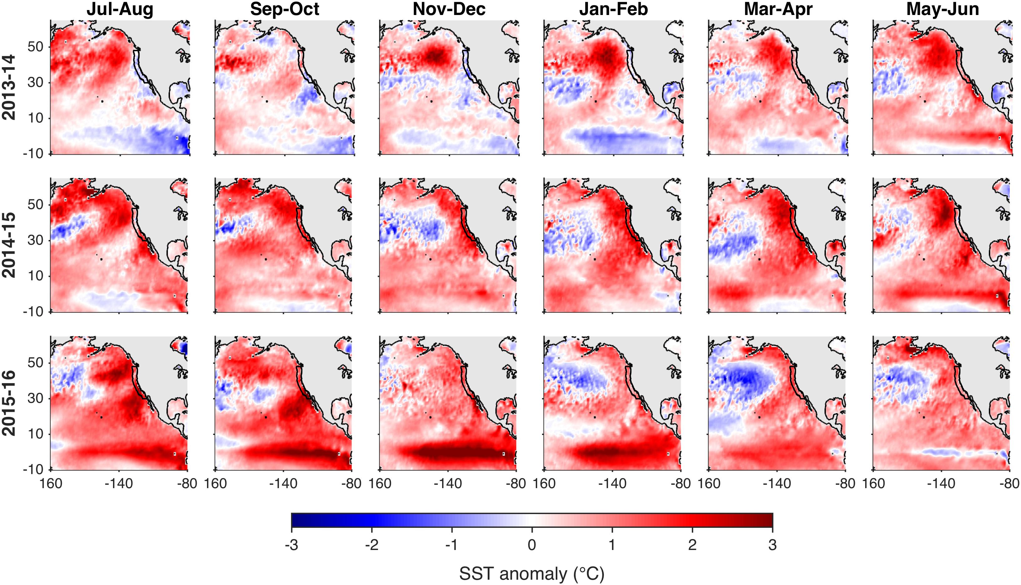
Figure 1. Observed evolution of northeast Pacific SST anomalies from July 2013 to June 2016. Anomalies are calculated relative to the 1982–2010 climatology using the 0.25° OISSTv2 product. The CCS region of interest to this paper, extending along the North American west coast from 30 to 48°N and from the coast to 300 km offshore, is outlined in black.

While the CCS was persistently anomalously warm throughout 2014–2016 (Figure 1), regional and broad-scale anomalies during that period evolved in response to a suite of forcing mechanisms (Amaya et al., 2016) including (i) the “Ridiculously Resilient Ridge,” a blocking high pressure system (Swain et al., 2014) that gave rise to the Blob by reducing wind-driven mixing and wintertime cooling in the northeast Pacific (Bond et al., 2015), (ii) the subsequent impact of offshore warm anomalies on the CCS, likely through both lateral advection and anomalous atmospheric forcing (Zaba and Rudnick, 2016; Chao et al., 2017; Jacox et al., 2018), (iii) evolution from the Blob warming pattern characteristic of North Pacific Gyre Oscillation (NPGO) variability to an arc-pattern warming resembling Pacific Decadal Oscillation (PDO) variability, a transition that may have been facilitated by tropical-extratropical teleconnections through an El Niño event in 2014–2015 that was initially predicted to be very strong but ultimately was weak (McPhaden, 2015; Amaya et al., 2016; Di Lorenzo and Mantua, 2016), and (iv) the 2015–2016 El Niño event that was one of the strongest on record based on equatorial Pacific SSTa, but whose CCS expression was quite different from that expected based on past strong El Niños (Jacox et al., 2016; Frischknecht et al., 2017).

Advance warning of events like the 2014–2016 CCS heatwave, whether it be for the onset of anomalous warming or its evolution thereafter, would enable ocean managers and other stakeholders to be proactive in their decision making. To that end, the overarching aim of this paper is to determine what about this heatwave was predictable, and why. Hu et al. (2017) examined seasonal forecasts from the National Center for Environmental Prediction’s Climate Forecast System (NCEP-CFSv2) to assess predictions in the region of the Blob, centered on ∼140°W, 45°N (see November–December 2013 in Figure 1). They found little forecast skill for the initiation of this extreme warm anomaly, which was forced by atmospheric internal variability that is inherently unpredictable. However, anomalous warming of the CCS occurred following the establishment of the offshore warm anomaly, and so prediction of CCS anomalies was not necessarily limited in the same way. It is conceivable that while the Blob was not predictable, subsequent impacts on the CCS were; such is the case for El Niño – Southern Oscillation (ENSO) events that once developed in the tropics can impart predictability in the CCS for the following months (Doi et al., 2015; Jacox et al., 2017).

Here, we explore seasonal forecasts from eight global climate forecast systems that have contributed to the North American Multi-Model Ensemble (NMME; Kirtman et al., 2014) and assess their ability to predict different phases of the 2014–2016 CCS warm anomalies. We examine variability averaged over the CCS domain as well as the spatial evolution of forecast and observed SST anomalies in the northeast Pacific, and link the success or failure of model forecasts to the mechanisms responsible for the SSTa variability. Finally, we combine individual ensemble members from each model to create a large (85-member) forecast ensemble, which can indicate the probability of extreme warm anomalies even when they are largely missed by ensemble mean forecasts.

Materials and Methods

Seasonal Forecasts

Seasonal SST forecasts are obtained from global coupled climate models contributing to the NMME. We focus on eight models whose SST forecasts are publicly available for a long re-forecast period as well as for the recent years that are the focus of this study (i.e., 1982–2016). The models are CMC1-CanCM3 and CMC2-CanCM4 (Merryfield et al., 2013) from the Canadian Meteorological Center (CMC), NCEP-CFSv2 (Saha et al., 2014) from the National Center for Environmental Prediction (NCEP), COLA-RSMAS-CCSM4 (Infanti and Kirtman, 2016) from the National Center for Atmospheric Research (NCAR), GFDL-CM2p1-aer04 (Delworth et al., 2006), GFDL-CM2p5-FLOR-A06 (Vecchi et al., 2014), and GFDL-CM2p5-FLOR-B01 (Vecchi et al., 2014) from the Geophysical Fluid Dynamics Laboratory (GFDL), and NASA-GMAO-062012 (Vernieres et al., 2012) from the National Aeronautics and Space Administration (NASA). For each model, forecasts are initialized monthly and an ensemble of forecasts is produced. For all models except CFSv2, forecasts are initialized on the first day of the month and an ensemble of 10–12 members is produced at each initialization time. Individual ensemble members are generated by introducing small perturbations to the initial conditions, which grow in time to large differences due to the chaotic nature of the climate system (Lorenz, 1963). For CFSv2, four ensemble members are initialized every fifth day, for a total of 24 per month. For consistency with other models, we use only 10 ensemble members from CFSv2, the four initialized on the first of the month and the last six initialized the previous month. Monthly average output is saved for lead times from 0 (e.g., a January 1^st forecast of mean January conditions) to 11 months, except for the CFSv2 and NASA-GMAO models, which have forecasts available for lead times up to 8 months.

Skill Evaluation

As global climate models have in some cases large SST biases, especially in eastern boundary upwelling systems like the CCS, forecasts must be bias corrected for comparison with observations. Additionally, models drift from their initialized state toward their preferred (biased) state over the course of a forecast, so bias correction is initialization month- and lead time-dependent. For each initialization month and lead time, forecast SST anomaly (SSTa) is computed by removing the 1982–2010 forecast climatology, and observed SSTa is calculated similarly by removing the 1982–2010 climatology from NOAA’s 0.25° Optimum Interpolation SST, version 2 (OISSTv2; Reynolds et al., 2007; Banzon et al., 2016). This method assumes that forecast biases are stationary in time, which is an oversimplification (Supplementary Figure 1; Kumar et al., 2012). However, there is no established protocol for dealing with non-stationarity in forecast biases. We discuss this issue more in Section “California Current System SST Anomalies,” particularly with reference to the NCEP-CFSv2 forecasts.

We evaluate SSTa forecasts with respect to observed conditions in the CCS, which we defined as extending 30–48°N and from the coast to 300 km offshore, as well as in the broader northeast Pacific (Figure 1). Past analyses of NMME forecast SSTa (Stock et al., 2015; Hervieux et al., 2017; Jacox et al., 2017) have relied on several skill metrics for evaluation: the deterministic metrics anomaly correlation coefficient (ACC) and root mean square error (RMSE), and the probabilistic Brier Score. In each case, skill scores have been calculated based on interannual variability over a long (∼30-year) time series. Such analyses have demonstrated that NMME forecasts have significant skill for SSTa in the CCS at lead times of at least 5 months and up to 11 months depending on initialization month. Furthermore, NMME SSTa forecasts outperform persistence forecasts in the CCS, primarily due to the ability of the model forecasts to capture anomalies associated with moderate to strong ENSO events (Jacox et al., 2017). While long-term skill assessments offer a baseline evaluation of model forecasts capabilities, here we aim to evaluate predictions for individual fluctuations over a much shorter time period (3 years), so the same skill metrics are not appropriate. Instead, we focus on the SSTa forecast error (forecast minus observed SSTa) to evaluate predictions of mean CCS conditions and spatial anomaly correlations to evaluate the ability of models to predict the spatial evolution of SSTa more broadly in the northeast Pacific.

Persistence Forecasts

We use a “damped persistence” forecast as a baseline against which to evaluate the skill of model forecasts. The damped persistence forecast assumes that observed SSTa decays toward zero over some characteristic timescale, and it is a more rigorous baseline for forecast skill than the climatology (which has zero skill for predicting anomalies) or a simple persistence forecast (which unrealistically maintains anomalies in the absence of additional forcing) (e.g., Mason and Mimmack, 2002). The damped persistence forecast SSTa at lead t is calculated from SSTa(t) = aSSTa(i), where SSTa(i) is the observed SSTa at forecast initialization and a is the autocorrelation coefficient of SSTa at lag t.

Results

California Current System SST Anomalies

While warm SSTa generally persisted along the North American coast from early 2014 through at least 2016, on monthly timescales the CCS saw distinct periods of increasing and decreasing SSTa. Models were able to forecast some of these fluctuations with clear skill, while in other cases they performed no better than a damped persistence forecast (Figure 2). All models predicted increasing SSTa in late winter and early spring 2014, albeit this anomalous warming was more gradual in forecasts than in observations. A warmer than average 2014 early summer was predicted by all models with a January initialization, and the multi-model mean SSTa forecast for summer 2014 fell halfway between the persistence forecast (0°C) and the observed anomaly (0.8°C). However, a second pulse of anomalous warming in late 2014, which increased observed SSTa from 0.8 to 2°C, was absent from the January initialized forecasts. In fact, even forecasts initialized in July – approximately 2 months before this second period of rapid SSTa increase – predicted SSTa to decrease toward zero rather than increase. CCS temperatures remained elevated throughout much of 2015, interrupted only by a brief but strong cooling in May–June. This pattern was missed by forecasts initialized in January 2015, which generally predicted decreasing SSTa throughout the year following the damped persistence forecast. Finally, 2016 was characterized by yet another brief period of increased SSTa in spring followed by cool and warm SSTa in summer and fall, respectively. The spring 2016 warm period was captured with impressive fidelity by model forecasts, with the January initialized multi-model mean matching observations almost exactly through June (Figure 2), although forecast skill dropped off later in 2016.

FIGURE 2

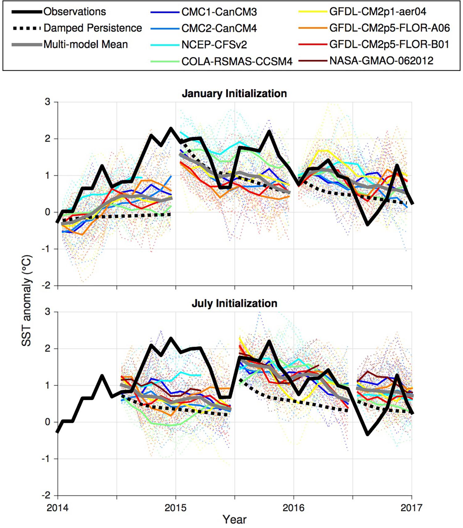
Figure 2. Global climate forecasts for mean SSTa in the CCS, initialized in (top) January and (bottom) July of each year from 2013 to 2016. Thin dotted colored lines are individual ensemble members for each model while solid colored lines are model means. For each model, anomalies are calculated relative to the lead time-and initialization month-dependent climatology.

The findings outlined above – that forecasts exhibited skill for SSTa changes in early 2014 and early 2016, but not for mid-2014 through 2015 – generally hold true across models and lead times (Figure 3). For longer leads (e.g., 8 months), skillful forecasts of early 2014 anomalous warming led to improvements over a damped persistence forecast throughout 2014, and in fact the multi-model mean forecast outperformed a damped persistence forecast for much of the study period. However, the most intense warm anomalies in late 2014 were largely missed by all models even at lead times of 2 months, as was the persistence of those anomalies into 2015. In contrast, the evolution of the early 2016 warm period, with SSTa exceeding 1°C, was forecast with very high skill even 8 months in advance (Figure 3). Forecasts from individual models differ quantitatively but exhibit skill during the same time periods, consistent with findings for large marine ecosystems around the U.S. and elsewhere (Stock et al., 2015; Hervieux et al., 2017).

FIGURE 3

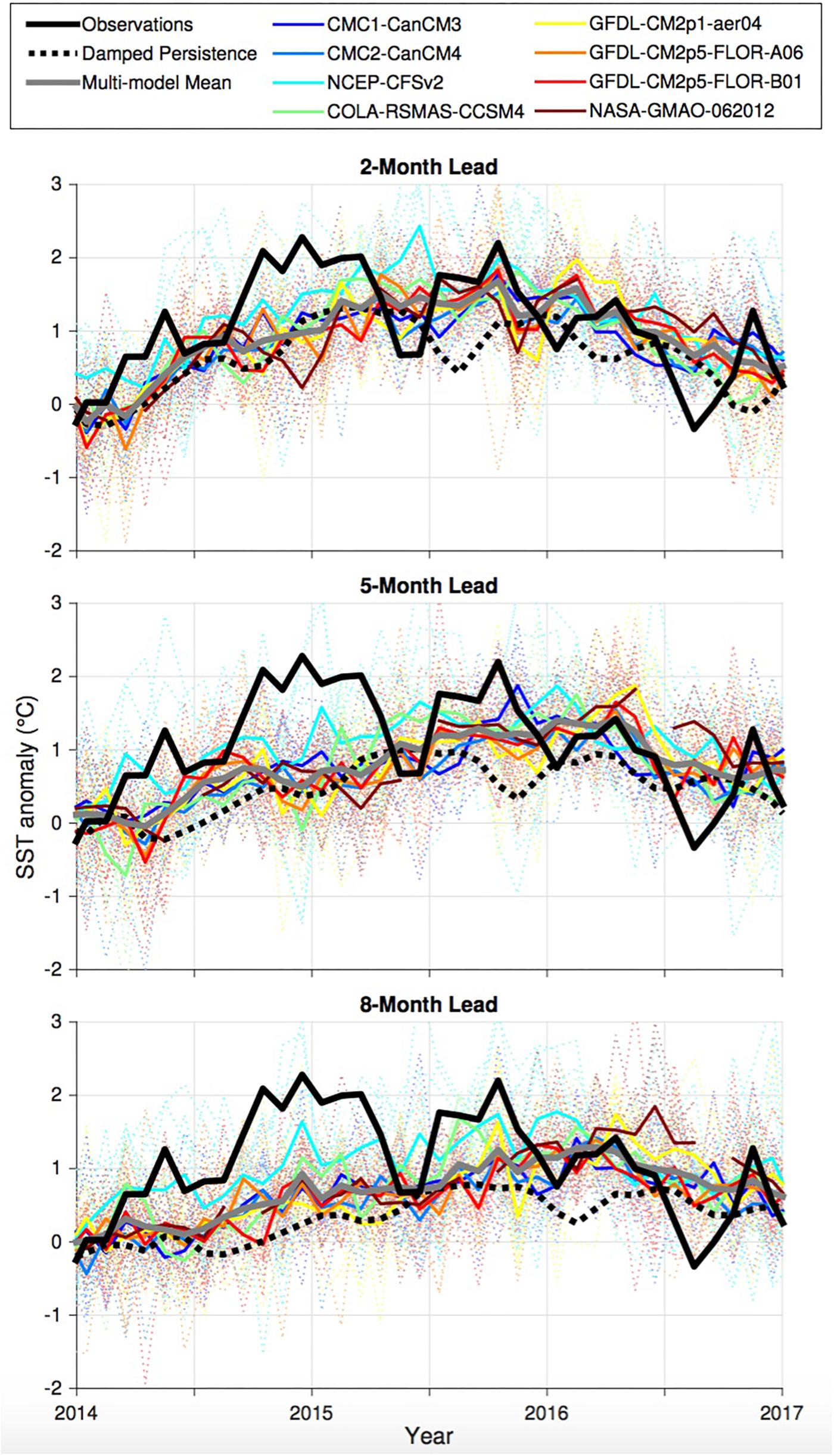
Figure 3. Global climate forecasts for SSTa in the CCS at multiple lead times. Forecasts are initialized monthly. Lines are as in Figure 2.

One model, NCEP-CFSv2, emerges as a potential outlier with forecast SSTa that is in some cases much higher than that seen in other models (Figure 2). However, interpretation of this result is challenging for several reasons. First, CFSv2 anomalies are warmer than those of other models throughout 2013–2016, not just during the observed warm periods (e.g., see 8-month lead forecasts in Figure 3), suggesting an issue with the bias correction. As mentioned earlier, anomalies are calculated relative to a 1982–2010 climatology but in fact biases change over time. The non-stationarity of CFSv2 biases was noted by Kumar et al. (2012), in particular with regards to an apparent shift to warmer biases around 1999. While this issue is not unique to CFSv2 (all models have state-dependent biases), the CFSv2 warm bias has increased relative to other models over time, especially since ∼2007 (Supplementary Figure 1). Second, the CFS Reanalysis that is used to initialized CFSv2 forecasts had a prominent tropical Atlantic cold bias that developed in October 2013 and was addressed in March 2016. The cold Atlantic bias resulted in a persistent El Niño-like state, favoring warm anomalies in the northeast Pacific (NOAA/NCEP Climate Prediction Center, 2015, 2016a,b).

Northeast Pacific Spatial SST Anomalies and Forcing

To further explore and contextualize the CCS anomalies described in the previous section, we turn our attention to the spatial evolution of observed and forecast SSTa in the broader northeast Pacific, taking the years 2014, 2015, and 2016 in turn. We focus initially on the multi-model mean forecast, as forecasts for individual models differ quantitatively but display similar structure. We discuss observed anomalies and the ability of models to forecast them here, and in the discussion we link these findings to the mechanisms that may have imparted increased predictability to early 2014 and early 2016 relative to late 2014 and 2015.

In the observations, 2014 was characterized by an intense offshore warm anomaly evolving into an arc warming pattern with concomitant increases in CCS SSTa (Figure 1). As we have seen previously this anomalous 2014 warming occurred in two stages, one in early 2014 that was also seen in model forecasts and another in late summer/fall that was not. The early 2014 SSTa increase occurred by an expansion of the offshore warm anomaly to the coast, which was forecast in the multi-model mean (Figure 4), albeit with a lag of several months relative to observations (May–June vs. March–April). Thus, while the formation of the Blob itself was not predictable (Hu et al., 2017), its subsequent influence on the CCS was somewhat predictable.

FIGURE 4

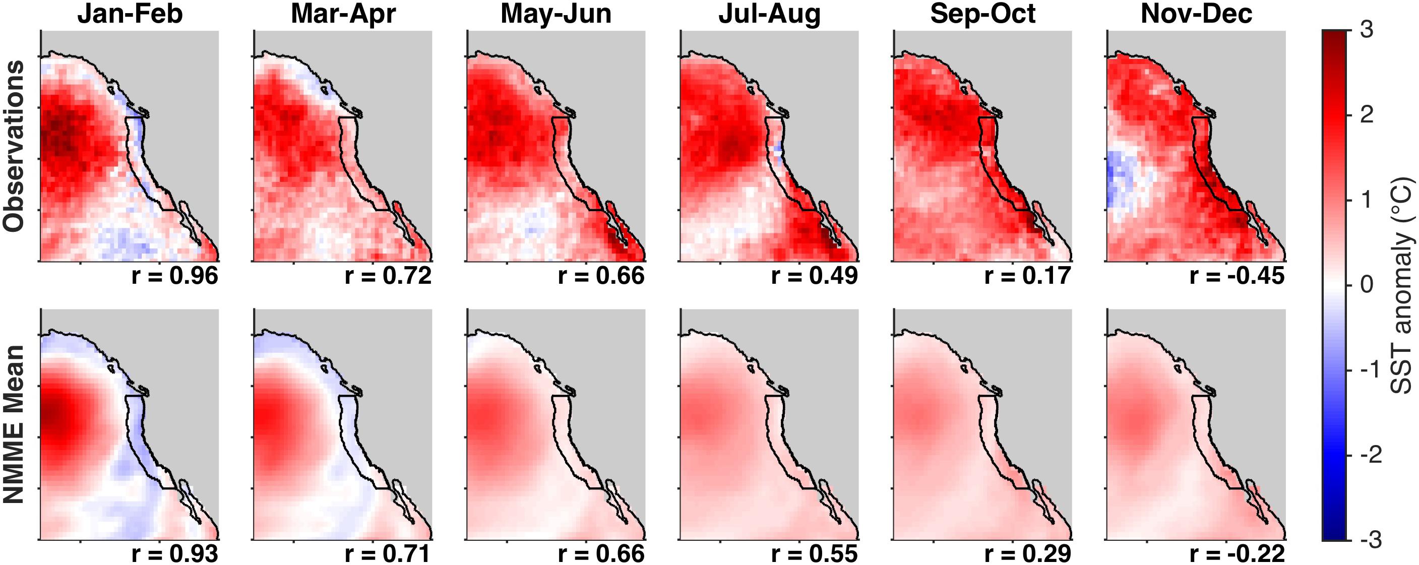
Figure 4. (Top) Observed and (bottom) forecast SSTa for 2-month periods throughout 2014. Forecasts were initialized in January. Correlation coefficients in top panels are for persistence forecasts, correlation coefficients in bottom panels are for NMME multi-model mean forecasts. The CCS region is outlined in black.

The SSTa increase of late 2014 had a very different character from that early in the year, as the spatial structure of northeast Pacific SSTa transitioned from a North Pacific Gyre Oscillation (NPGO)-like pattern with anomalies centered in the Gulf of Alaska to a Pacific Decadal Oscillation (PDO)-like arc pattern with warm anomalies along the North American coast and cold anomalies in the gyre (Di Lorenzo and Mantua, 2016). In contrast to the early part of the year, late 2014 was not characterized by clear forecast skill for the additional anomalous warming, though forecast anomalies from earlier 2014 persisted and provided model forecast skill superior to a damped persistence forecast (Figure 2). Also notable in the spatial anomaly forecasts is that forecast SSTa are muted relative to observations; in the ensemble mean forecast biases from individual ensemble members cancel each other, reducing the ensemble mean forecast variance especially at longer leads (e.g., Doblas-Reyes et al., 2005).

In 2015, the CCS remained very warm with persistent SSTa near 2°C, interrupted only by a brief cooling in May–June that while dramatic in CCS time series (Figure 2) was a very localized event in the northeast Pacific (Figure 5) driven by an anomalously strong spring 2015 upwelling season (Peterson et al., 2017). Spatial correlations for both model and persistence forecasts were briefly reduced during this late spring/summer cooling before returning to relatively high levels (r ≈ 0.5), supporting the notion that it was a brief interruption of a persistent warm period rather than a shift to a new and distinct warm event.

FIGURE 5

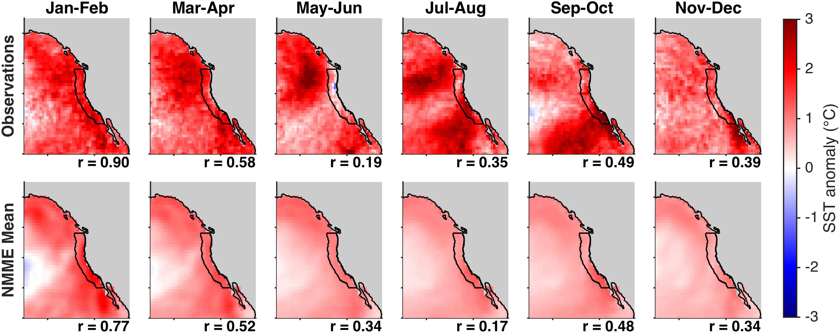
Figure 5. As in this image, but for 2015.

Finally, by late 2015 the equatorial Pacific was experiencing by some metrics (e.g., NOAA’s Oceanic Niño Index) one of the strongest El Niños on record. While its impact on the CCS was not as strong as expected based on tropical Pacific SSTa (Jacox et al., 2016), a moderate SSTa increase in spring 2016 was evident (Figures 2, 6). Model forecasts for this period were highly accurate, and much better than damped persistence, for both the CCS averaged SSTa (Figure 2) and spatial SSTa (Figure 6).

FIGURE 6

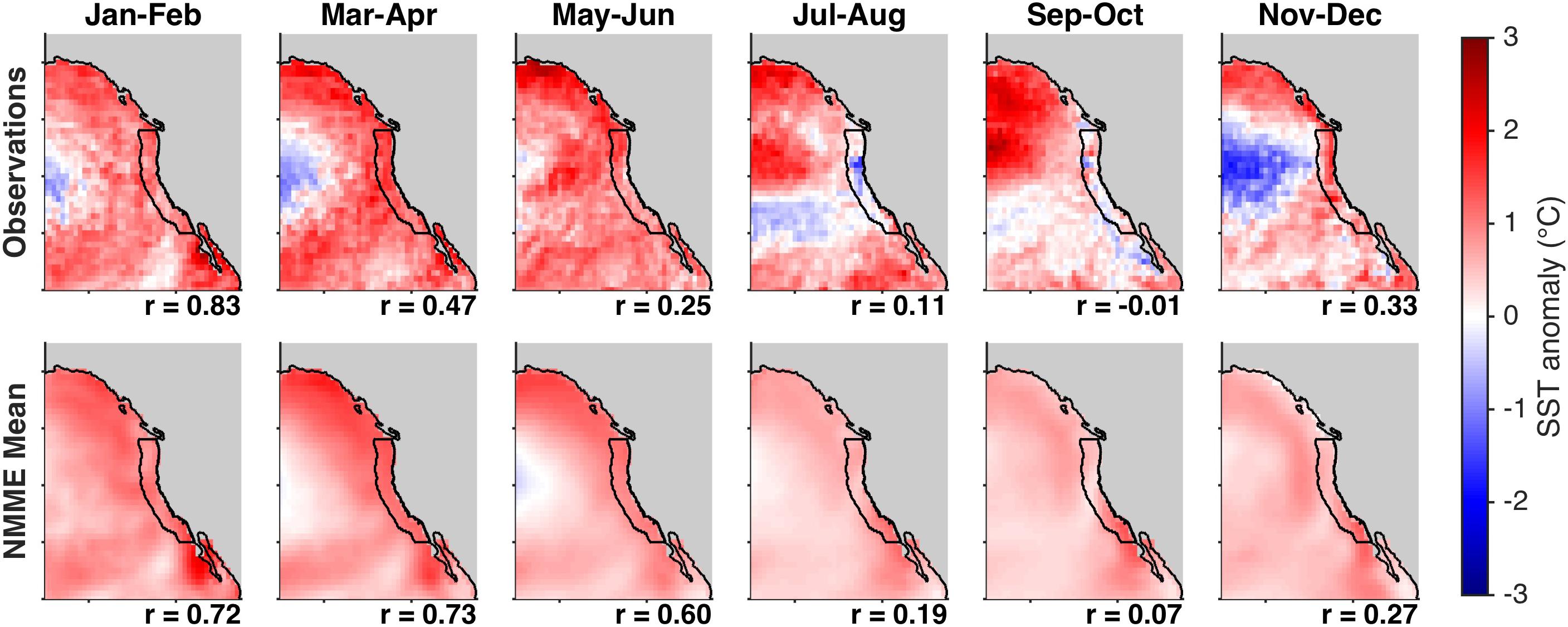
Figure 6. As in Figure 5, but for 2016.

In general, forecast errors for the mean CCS SSTa (Figure 2) mirror spatial anomaly correlations computed over the northeast Pacific (Figure 7). In other words, when forecast errors for the CCS are small, the structure of anomalies in the broader northeast Pacific tends to also be skillfully forecast. Given that our CCS region occupies a relatively small fraction of the northeast Pacific, this result is not obvious. It suggests that when CCS forecasts are skillful, their skill derives from accurate representation of the large-scale dynamics.

FIGURE 7

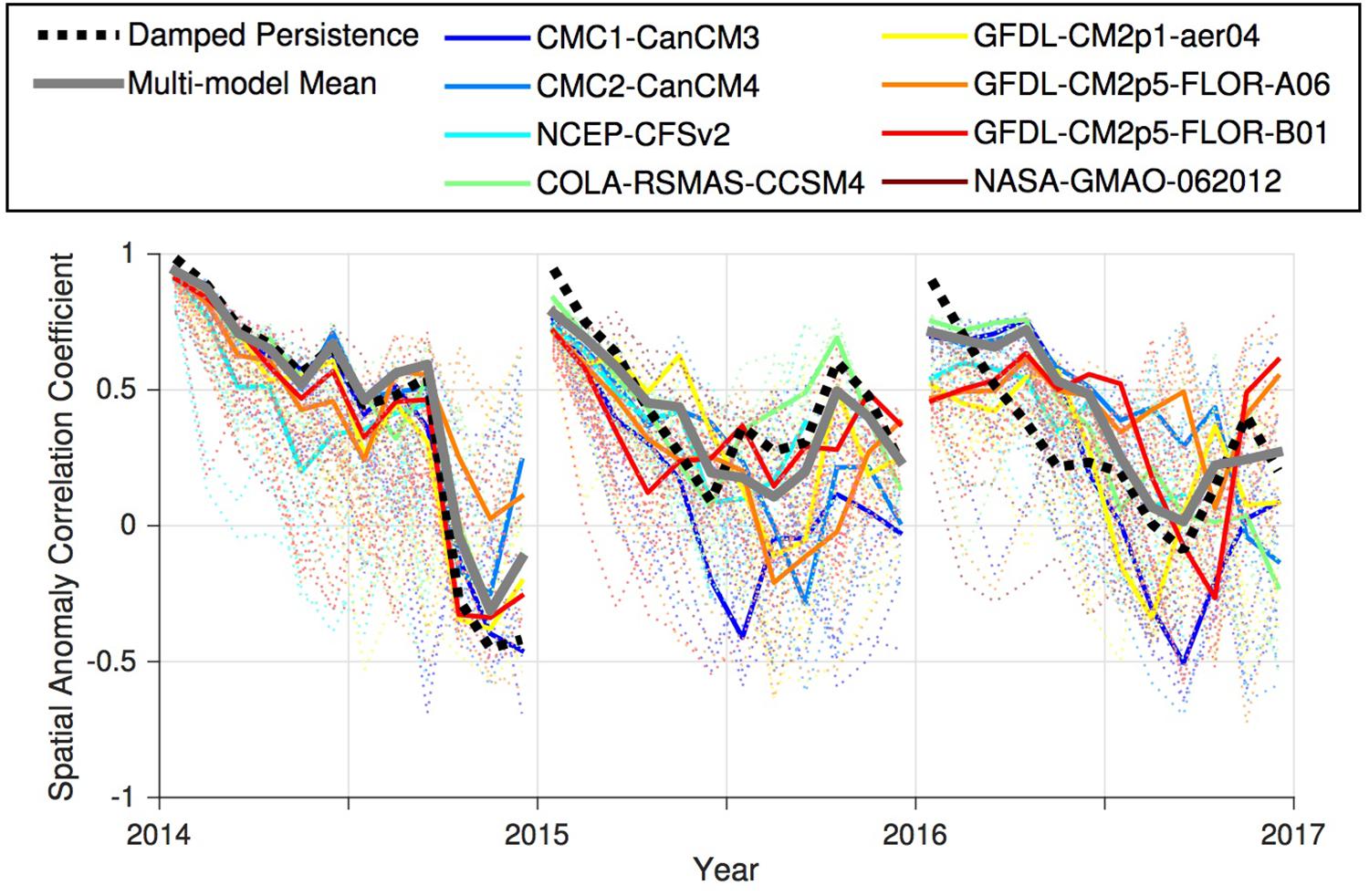
Figure 7. Spatial anomaly correlation coefficients for January-initialized forecasts. At each lead time, anomaly correlation coefficients were calculated between forecast and observed SSTa for the area plotted in Figure 5 (150–105°W, 20–65°N). Lines are as in Figure 2.

A Large Ensemble of Forecasts

To this point we have focused our analysis on NMME multi-model mean forecasts or mean forecasts for individual climate models. Overall, ensemble mean forecasts outperformed damped persistence forecasts in the 2013–2016 period, and during the peak warm anomalies from mid-2014 to the end of 2015, 8-month lead multi-model mean forecasts outperformed damped persistence in 100% of months, with a substantially lower mean forecast error (0.8 vs. 1.2°C). However, since extreme events are by definition in the tails of probability distributions, large ensembles (50–100 members) may be required to forecast them (Doi et al., 2019). It is rare for a single modeling center to produce such an ensemble, but through the NMME we can obtain one. Combining ensemble members from each of the 8 models included in this study, we have a total of 85 ensemble members for each forecast initialization, which can be used to generate forecast plumes for the focal years of this study (Figure 8).

FIGURE 8

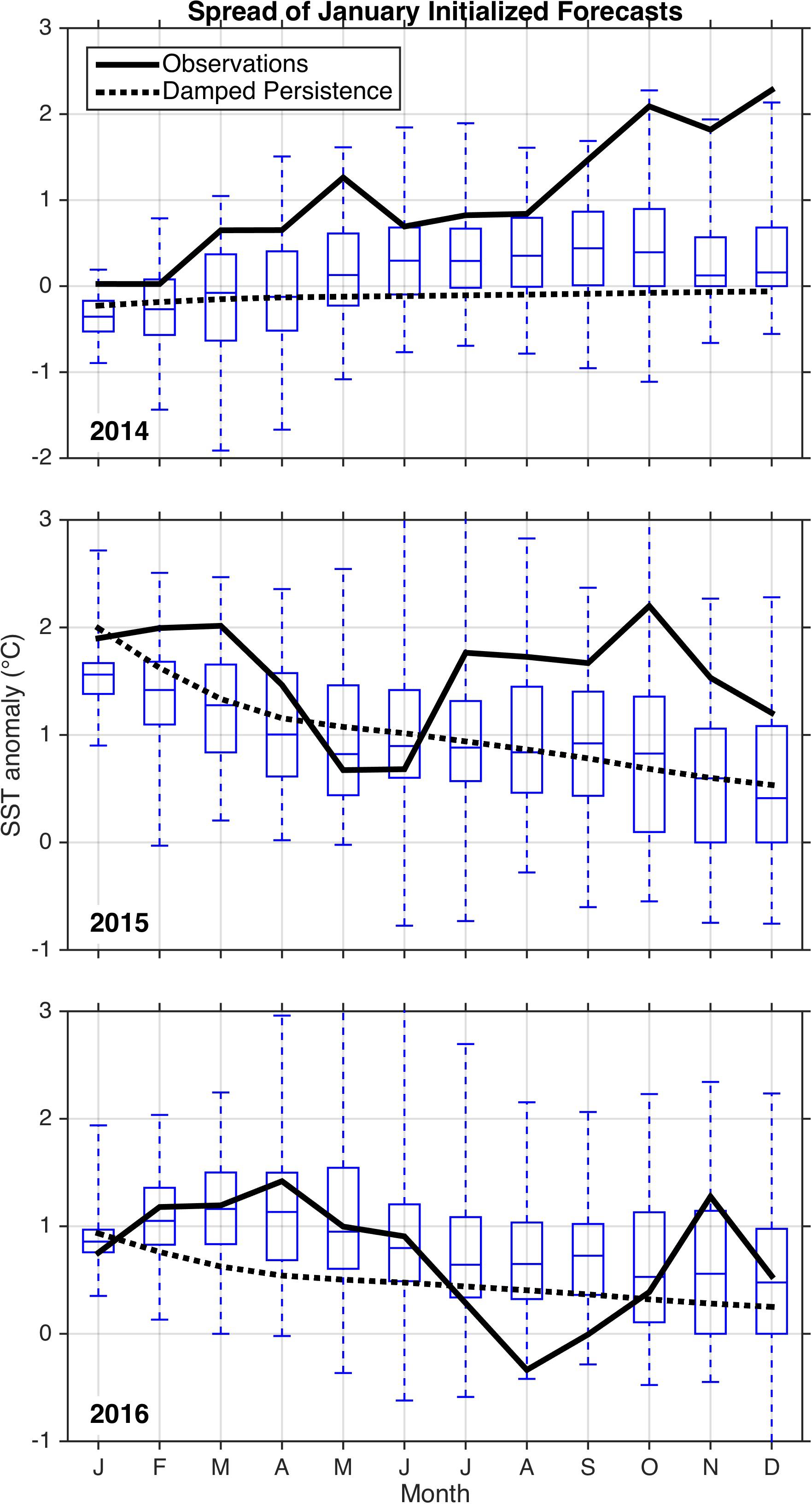
Figure 8. Forecast spread for January initialized forecasts of 2014, 2015, and 2016. For each panel, a total of 85 individual runs (10–12 runs from each of 8 models) are represented by box and whisker plots indicating the range and quartiles for each forecast month.

While model mean forecasts often evolve similarly in space and time (e.g., Supplementary Figure 2), individual ensemble members from a single model can differ dramatically (Supplementary Figure 3) such that the large ensemble forecast spread is regularly 3°C or more (Figure 8). While the multi-model ensemble mean forecast and the damped persistence forecast underestimated late 2014 and early 2015 SSTa by ∼1.5 and 2°C, respectively, the observed extremes were still within the ensemble spread at 8-month lead (Figure 9). Thus, this heatwave was forecast as an unlikely event, but not an impossible one. Furthermore, 8-month lead forecasts indicated elevated potential for extreme SSTa starting in mid-2014. The percentage of ensemble members forecasting SSTa greater than 2 standard deviations above the climatology (SSTa ≥∼1.4°C) rose from the long term mean value of approximately 3% to over 10% by late 2014 and upwards of 30% for late 2015 – early 2016 (Figure 9). The only other time in the past 35 years when this extreme positive SSTa forecast probability exceeded 10% was in early 1998, following the peak of one of the strongest El Niños on record.

FIGURE 9

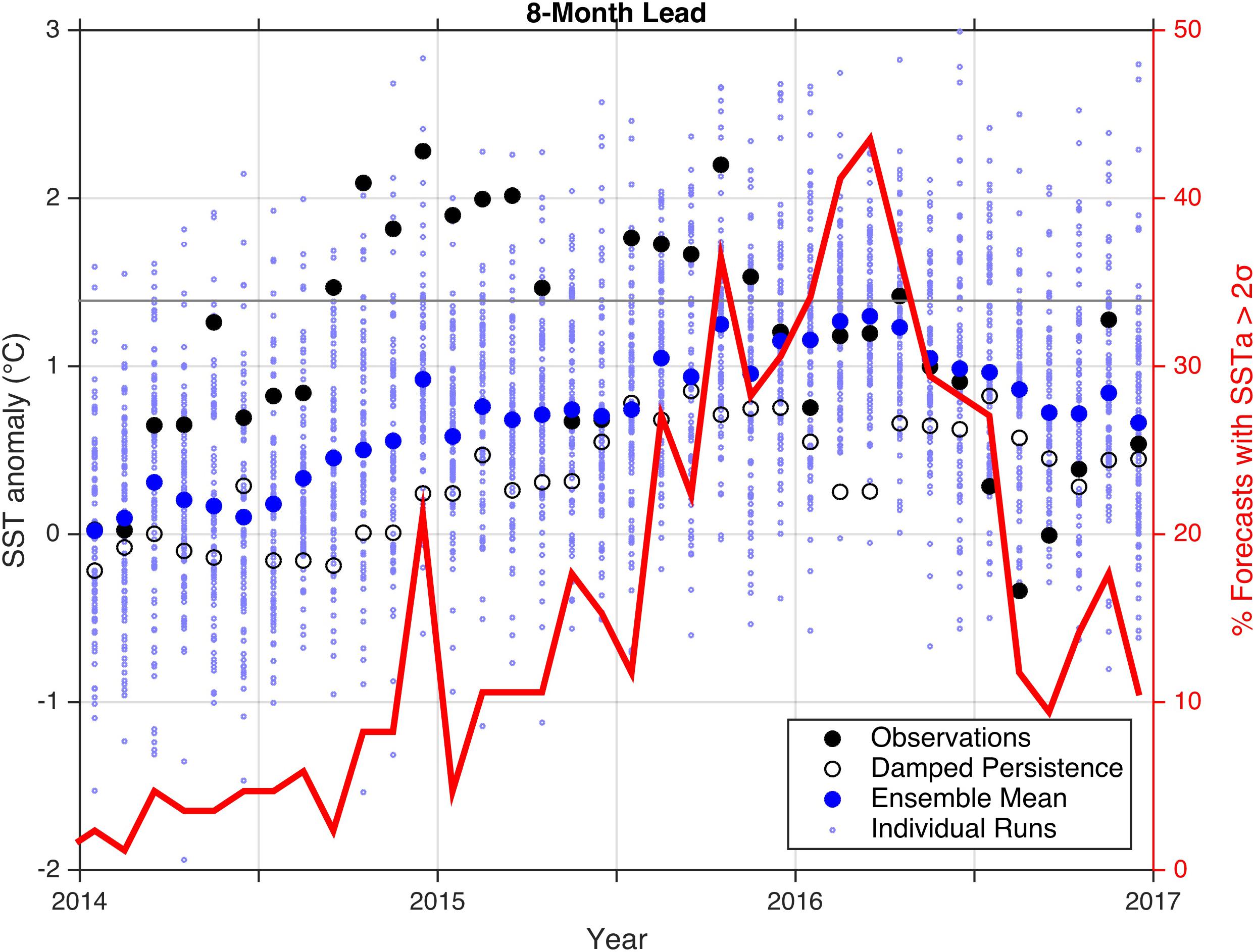
Figure 9. Monthly initialized 8-month lead forecasts are shown for each of 85 ensemble members taken from 8 models (small blue markers), the multi-model ensemble mean (large blue markers), a damped persistence forecast (open black circles), and observations (filled black circles). The red line shows the percentage of ensemble members with forecast SSTa greater than 2σ (∼1.39°C) for each forecast. The standard deviation (σ) was calculated from 1982 to 2017 observed SSTa and is marked by a thin gray line.

Discussion

Forcing Mechanisms and Predictability of 2014–2016 Heatwave

In the previous section, we evaluated global climate forecast system predictions of the evolving 2014–2016 CCS warm anomalies. Here, we put those predictions, and their success or failure, in the context of the mechanisms driving the SST fluctuations.

Rapidly increasing SSTa in the CCS in 2014 appears to have been driven by the evolution of pre-existing warm anomalies offshore toward the coast, consistent with a lagged response of the CCS to Gulf of Alaska SSTa (Jacox et al., 2018). This period of warming was forecast by models with some skill, though slightly lagged and with reduced magnitude relative to observations. Based on a heat budget analysis of a regional ocean model, Chao et al. (2017) attributed the early 2014 upper ocean temperature increase in the central CCS to a combination of anomalous surface heat fluxes and oceanic influence from the west, and Zaba and Rudnick (2016) found anomalous surface heat flux to be a dominant driver of anomalous warming in the southern CCS in the first half of 2014. Thus, a plausible explanation for forecast skill during this period is that the offshore anomalies present at initialization were conveyed to the CCS through the mean currents (i.e., eastward advection of offshore warm anomalies) and/or winds (i.e., westerlies transmitting anomalous surface heat fluxes after blowing over warm ocean anomalies upstream).

A second period of anomalous warming in late 2014 was not captured in model forecasts. During this period, the northeast Pacific SSTa pattern evolved from the “Blob” pattern with warm anomalies centered on the Gulf of Alaska to an arc pattern warming characteristic of the PDO. The positive PDO-like phase is typically characterized by anomalous northward winds and consequently reduced upwelling (or increased downwelling), which has been implicated in the anomalous CCS warming during this period (Zaba and Rudnick, 2016; Chao et al., 2017; Jacox et al., 2018). However, wind-stress driven SST anomalies along the North American west coast tend to be forecast skillfully only when they are associated with moderate to strong ENSO events (Doi et al., 2015; Jacox et al., 2017), and the lack of forecast skill in late 2014 (Figures 2, 4) is consistent with the neutral or weakly positive ENSO state.

Warm anomalies persisted through much of 2015 with a brief but strong cooling in late spring/early summer due to anomalously strong coastal upwelling (Peterson et al., 2017), which was not predicted in model forecasts. Consistent with regional upwelling being the dominant influence in this period, a regional heat budget identified vertical entrainment as the primary driver of SSTa fluctuations during 2015 (Chao et al., 2017). Remote ocean influence from the developing 2015–2016 El Niño likely also influenced the CCS in fall 2015, especially in the south (Frischknecht et al., 2017), but does not appear to have generated any appreciable forecast skill. As for late-2014, the mid-2015 variability was driven primarily by wind stress anomalies not associated with an ENSO event, so it is unsurprising that it was not predicted in the global forecasts (Jacox et al., 2017).

After a reduction of SSTa in the last months of 2015, another warm period in early 2016 was forecast with impressive skill. This last SSTa increase has been attributed to the 2015–2016 El Niño event via coastal waves and potentially anomalous poleward advection from the south (Chao et al., 2017). Winds in winter 2015–2016 were anomalously upwelling favorable, in contrast to the canonical El Niño response (Jacox et al., 2016), so the atmospheric teleconnection associated with ENSO variability does not appear to have imparted predictability in this case. The fact that the predictable influence of the 2015–2016 El Niño appears to have come through the oceanic pathway suggests that global models contain some representation of ENSO-forced coastal propagation even though they are too coarse to resolve coastal waves and currents (Capotondi et al., 2005).

By analyzing the spatiotemporal evolution of SSTa in concert with published findings on the forcing of these anomalies, we have developed hypotheses for why different phases of the 2014–2016 CCS heatwave were or were not predictable. Our analysis has focused on SST primarily for practical reasons, as the suite of variables publicly available in NMME output for recent years does not include the comprehensive diagnostics required for a full heat budget. Further exploration of these hypotheses, using heat budgets calculated from oceanic and atmospheric fluxes in model forecasts, is needed.

Ensemble Forecasts of SST Extremes

Multi-model ensemble mean forecasts outperformed damped persistence forecasts for much of the study period in terms of both forecast error and spatial anomaly correlations. During the most extreme warm anomalies in 2014 and 2015, model forecasts were consistently better than damped persistence, which had ∼50% higher mean forecast error. However, neither ensemble mean forecasts nor damped persistence forecasts predicted SSTa anywhere near those observed at their peak. We see two reasons for this discrepancy: first, the ensemble spread for individual forecasts tends to be quite large (Figure 8), such that bias cancelation in the ensemble mean produces much reduced variance in forecasts relative to observations, especially at longer lead times (e.g., Figures 4–6). This reduced variance does not affect skill metrics based on correlation, but does impact the forecast error. One potential remedy is to scale the ensemble mean variance such that forecasts at each lead time maintain the same variance as that in the observations or the zero-lead forecasts (i.e., variance inflation; Doblas-Reyes et al., 2005). Second, an ensemble mean forecast that captures the observed magnitude of an extreme event requires that a large portion of individual ensemble members agrees on the extreme forecast, which in turn requires that its forcing be primarily deterministic and that model forecasts accurately represent that deterministic forcing. However, we know that internal variability can also strongly influence seasonal forecasts, leading to a wide range of forecast outcomes (Figures 8, 9 and Supplementary Figure 3). Thus, a failed forecast could result either from unpredictable intrinsic variability or from the inability of a model forecast to capture a deterministic pathway (e.g., tropical-extratropical teleconnections proposed by Di Lorenzo and Mantua (2016) for the evolution of SSTa in 2015).

For both 2014 and 2016, the ratio of predictable components (Scaife and Smith, 2018) was greater than 1 (1.28 and 1.90, respectively), meaning that the correlation between the ensemble mean forecast and observations (r = 0.71 and 0.63, respectively) was stronger than the average correlation of the ensemble mean with individual ensemble members. Forecasts for these years were underconfident, as the ensemble mean forecast was better than what would be expected from the low model signal-to-noise ratio (Eade et al., 2014; Scaife and Smith, 2018). This is evidence of the “signal-to-noise paradox,” previously documented for ensemble climate predictions in the North Atlantic (Scaife and Smith, 2018). Scaife and Smith (2018) suggest that this underestimation of the signal-to-noise ratio in climate predictions may result from teleconnections, and their associated predictable signals, being too weak in climate models. Errors in the model signal-to-noise ratio can have a range of consequences that should be considered in forecast skill assessment, and post-processing techniques have been developed to correct for these errors (e.g., Eade et al., 2014).

Finally, rather than relying on ensemble mean forecasts to capture extremes, one can leverage the statistics of a large ensemble, which will contain members with low forecast error and high spatial correlations even when the ensemble mean predictions fail (Figures 7–9 and Supplementary Figures 2, 3). Model ensembles have been shown to improve probabilistic skill scores relative to single model forecasts (Hagedorn et al., 2005), including for warm/neutral/cool SSTa terciles along North American coasts (Hervieux et al., 2017). Given that skillful SSTa forecasts in the CCS appear to correspond to accurate representation of the broader-scale SSTa structure (i.e., low forecast errors in the CCS are associated with high spatial correlations in the northeast Pacific), one can speculate that the more skillful ensemble members are also predicting the mechanisms driving those anomalies more faithfully (i.e., they are right for the right reasons). However, such a hypothesis needs to be confirmed by comparing the heat budgets in successful and failed forecasts.

Regional Downscaling of Ocean Forecasts

One notable limitation of the climate forecast systems analyzed herein is their coarse resolution and resultant inability to resolve fine-scale ocean processes and features that are key to the functioning of the CCS and other systems. As a result, there are a number of ongoing efforts to improve regional forecasts through dynamical downscaling of global forecasts (e.g., Siedlecki et al., 2016). In such a configuration, output from global models such as those in the NMME are used as surface and lateral boundary conditions to regional ocean models that have 1–2 orders of magnitude higher resolution. Downscaled models have the advantage of being able to resolve important ocean dynamics that are sub-grid scale in global models (e.g., coastal upwelling, currents, eddies, and trapped waves). However, the downscaled model is ultimately dependent on the global model to impart forecast skill through surface or boundary forcing. For events where there is forecast skill derived from a clear deterministic pathway (e.g., surface fluxes and/or lateral advection in early 2014, poleward-propagating coastal trapped waves and/or anomalous advection in early 2016), a downscaled forecast or small ensemble of downscaled forecasts will better represent the fine scale impacts. On the other hand, for extreme events that result from unpredictable internal variability and can only be predicted in a probabilistic sense (e.g., wind driven SSTa variability in late 2014 and 2015), a downscaled ensemble of adequate size is currently computationally prohibitive and a large ensemble of global forecasts is the more appropriate tool (Doi et al., 2019).

Conclusion

An ongoing shift toward ecosystem-based management of the oceans (Levin et al., 2009; McLeod and Leslie, 2009) requires that information on the ocean state be accurate and readily available. The need for this information is even more pronounced in light of climate extremes that leave managers, fishers, and other stakeholders scrambling to adapt to rapid change. For one such extreme, the CCS marine heatwave of 2014–2016, we have outlined aspects of the ocean temperature evolution that were predictable in a deterministic sense, and others that were forecast with low probability in a large ensemble of seasonal forecasts. Incorporating ocean forecasts into management plans is a difficult task, complicated by inherent unpredictability in the climate system, an added layer of uncertainty when translating physical changes to ecological impacts, and questions surrounding the decision making process (e.g., at what probability of an extreme event is a management action initiated?). However, to the extent that skillful forecasts of ocean conditions can improve decision making relative to that possible with ocean monitoring alone (Payne et al., 2017; Tommasi et al., 2017), our findings offer hope for more effective management when forecasted marine heatwaves ultimately do transpire.

Data Availability

The NMME System Phase II data (https://www.earthsystemgrid.org/search.html?Project=NMME) were obtained from http://iridl.ldeo.columbia.edu/SOURCES/.Models/.NMME/. NOAA High Resolution SST data were provided by the NOAA/OAR/ESRL PSD, Boulder, CO, United States, from their website at https://www.esrl.noaa.gov/psd/.

Author Contributions

DT conceived the study. MJ, DT, MA, and CS designed the analysis. MJ performed the analysis with the help from GH and drafted the manuscript. All authors contributed to the writing of the manuscript.

Funding

Funding for this study was provided by the NOAA Modeling, Analysis, Predictions and Projections (MAPP) Program (NA17OAR4310108) and the NOAA/NMFS Office of Science and Technology.

Conflict of Interest Statement

The authors declare that the research was conducted in the absence of any commercial or financial relationships that could be construed as a potential conflict of interest.

Acknowledgments

This manuscript is a contribution of the NOAA Marine Prediction Task Force. We thank the two reviewers and the editor for their helpful suggestions to improve the manuscript. We acknowledge the agencies who supported the NMME-Phase II system. We also thank the climate modeling groups (Environment Canada, NASA, NCAR, NOAA/GFDL, NOAA/NCEP, and University of Miami) for producing and making available their model output. NOAA/NCEP, NOAA/CTB, and NOAA/CPO jointly provided the coordinating support and led the development of the NMME-Phase II system.

Supplementary Material

The Supplementary Material for this article can be found online at: https://www.frontiersin.org/articles/10.3389/fmars.2019.00497/full#supplementary-material

References

Amaya, D. J., Bond, N. E., Miller, A. J., and DeFlorio, M. J. (2016). The evolution and known atmospheric forcing mechanisms behind the 2013-2015 North Pacific warm anomalies. US Clivar Var. 14, 1–6.

Google Scholar

Banzon, V., Smith, T. M., Chin, T. M., Liu, C., and Hankins, W. (2016). A long-term record of blended satellite and in situ sea-surface temperature for climate monitoring, modeling and environmental studies. Earth Syst. Sci. Data 8, 165–176. doi: 10.5194/essd-8-165-2016

CrossRef Full Text | Google Scholar

Bond, N. A., Cronin, M. F., Freeland, H., and Mantua, N. (2015). Causes and impacts of the 2014 warm anomaly in the NE Pacific. Geophys. Res. Lett. 42, 3414–3420. doi: 10.1002/2015gl063306

CrossRef Full Text | Google Scholar

Capotondi, A., Alexander, M. A., Deser, C., and Miller, A. J. (2005). Low-frequency pycnocline variability in the northeast Pacific. J. Phys. Oceanogr. 35, 1403–1420. doi: 10.1175/jpo2757.1

CrossRef Full Text | Google Scholar

Cavole, L. M., Demko, A. M., Diner, R. E., Giddings, A., Koester, I., Pagniello, C. M., et al. (2016). Biological impacts of the 2013–2015 warm-water anomaly in the Northeast Pacific: winners, losers, and the future. Oceanography 29, 273–285.

Google Scholar

Chao, Y., Farrara, J. D., Bjorkstedt, E., Chai, F., Chavez, F., Rudnick, D. L., et al. (2017). The origins of the anomalous warming in the California coastal ocean and San Francisco Bay during 2014–2016. J. Geophys. Res. Oceans 122, 7537–7557. doi: 10.1002/2017jc013120

CrossRef Full Text | Google Scholar

Delworth, T. L., Broccoli, A. J., Rosati, A., Stouffer, R. J., Balaji, V., Beesley, J. A., et al. (2006). GFDL’s CM2 global coupled climate models. Part I: formulation and simulation characteristics. J. Clim. 19, 643–674.

Google Scholar

Di Lorenzo, E., and Mantua, N. (2016). Multi-year persistence of the 2014/15 North Pacific marine heatwave. Nat. Clim. Change 6:1042. doi: 10.1038/nclimate3082

CrossRef Full Text | Google Scholar

Doblas-Reyes, F. J., Hagedorn, R., and Palmer, T. N. (2005). The rationale behind the success of multi-model ensembles in seasonal forecasting—II. Calibration and combination. Tellus A Dyn. Meteorol. Oceanogr. 57, 234–252. doi: 10.1111/j.1600-0870.2005.00104.x

CrossRef Full Text | Google Scholar

Doi, T., Behera, S. K., and Yamagata, T. (2019). Merits of a 108-Member Ensemble system in ENSO and IOD predictions. J. Clim. 32, 957–972. doi: 10.1175/jcli-d-18-0193.1

CrossRef Full Text | Google Scholar

Doi, T., Yuan, C., Behera, S. K., and Yamagata, T. (2015). Predictability of the California Niño/Niña. J. Clim. 28, 7237–7249.

Google Scholar

Eade, R., Smith, D., Scaife, A., Wallace, E., Dunstone, N., Hermanson, L., et al. (2014). Do seasonal-to-decadal climate predictions underestimate the predictability of the real world? Geophys. Res. Lett. 41, 5620–5628. doi: 10.1002/2014gl061146

PubMed Abstract | CrossRef Full Text | Google Scholar

Frischknecht, M., Münnich, M., and Gruber, N. (2017). Local atmospheric forcing driving an unexpected California current system response during the 2015–2016 El Niño. Geophys. Res. Lett. 44, 304–311. doi: 10.1002/2016gl071316

CrossRef Full Text | Google Scholar

Gentemann, C. L., Fewings, M. R., and García-Reyes, M. (2017). Satellite sea surface temperatures along the West Coast of the United States during the 2014–2016 northeast Pacific marine heat wave. Geophys. Res. Lett. 44, 312–319. doi: 10.1002/2016gl071039

CrossRef Full Text | Google Scholar

Hagedorn, R., Doblas-Reyes, F. J., and Palmer, T. N. (2005). The rationale behind the success of multi-model ensembles in seasonal forecasting–I. Basic concept. Tellus A 57, 219–233. doi: 10.1111/j.1600-0870.2005.00103.x

CrossRef Full Text | Google Scholar

Hervieux, G., Alexander, M. A., Stock, C. A., Jacox, M. G., Pegion, K., Becker, E., et al. (2017). More reliable coastal SST forecasts from the North American multimodel ensemble. Clim. Dyn. 1–16. doi: 10.1007/s00382-017-3652-7

CrossRef Full Text | Google Scholar

Hobday, A. J., Oliver, E. C., Gupta, A. S., Benthuysen, J. A., Burrows, M. T., Donat, M. G., et al. (2018). Categorizing and naming marine heatwaves. Oceanography 31, 162–173.

Google Scholar

Hu, Z. Z., Kumar, A., Jha, B., Zhu, J., and Huang, B. (2017). Persistence and predictions of the remarkable warm anomaly in the northeastern Pacific Ocean during 2014–16. J. Clim. 30, 689–702. doi: 10.1175/jcli-d-16-0348.1

CrossRef Full Text | Google Scholar

Infanti, J. M., and Kirtman, B. P. (2016). Prediction and predictability of land and atmosphere initialized CCSM4 climate forecasts over North America. J. Geophys. Res. Atmos. 121, 12690–12701.

Google Scholar

Jacox, M. G., Alexander, M. A., Mantua, N. J., Scott, J. D., Hervieux, G., Webb, R. S., et al. (2018). Forcing of multiyear extreme ocean temperatures that impacted California current living marine resources in 2016. Bull. Am. Meteorol. Soc. 99, S27–S33.

Google Scholar

Jacox, M. G., Alexander, M. A., Stock, C. A., and Hervieux, G. (2017). On the skill of seasonal sea surface temperature forecasts in the California current system and its connection to ENSO variability. Clim. Dyn. 1–15. doi: 10.1007/s00382-017-3608-y

CrossRef Full Text | Google Scholar

Jacox, M. G., Hazen, E. L., Zaba, K. D., Rudnick, D. L., Edwards, C. A., Moore, A. M., et al. (2016). Impacts of the 2015–2016 El Niño on the California current system: early assessment and comparison to past events. Geophys. Res. Lett. 43, 7072–7080. doi: 10.1002/2016gl069716

CrossRef Full Text | Google Scholar

Kirtman, B. P., Min, D., Infanti, J. M., Kinter, J. L. III, Paolino, D. A., Zhang, Q., et al. (2014). The North American multimodel ensemble: phase-1 seasonal-to-interannual prediction; phase-2 toward developing intraseasonal prediction. Bull. Am. Meteorol. Soc. 95, 585–601. doi: 10.1175/bams-d-12-00050.1

CrossRef Full Text | Google Scholar

Kumar, A., Chen, M., Zhang, L., Wang, W., Xue, Y., Wen, C., et al. (2012). An analysis of the nonstationarity in the bias of sea surface temperature forecasts for the NCEP Climate Forecast System (CFS) version 2. Mon. Weather Rev. 140, 3003–3016. doi: 10.1175/mwr-d-11-00335.1

CrossRef Full Text | Google Scholar

Levin, P. S., Fogarty, M. J., Murawski, S. A., and Fluharty, D. (2009). Integrated ecosystem assessments: developing the scientific basis for ecosystem-based management of the ocean. PLoS Biol. 7:e1000014. doi: 10.1371/journal.pbio.1000014

PubMed Abstract | CrossRef Full Text | Google Scholar

Lorenz, E. N. (1963). Deterministic nonperiodic flow. J. Atmos. Sci. 20, 130–141. doi: 10.1175/1520-0469(1963)020<0130:dnf>2.0.co;2

CrossRef Full Text | Google Scholar

Mason, S. J., and Mimmack, G. M. (2002). Comparison of some statistical methods of probabilistic forecasting of ENSO. J. Clim. 15, 8–29. doi: 10.1175/1520-0442(2002)015<0008:cossmo>2.0.co;2

CrossRef Full Text | Google Scholar

McCabe, R. M., Hickey, B. M., Kudela, R. M., Lefebvre, K. A., Adams, N. G., Bill, B. D., et al. (2016). An unprecedented coastwide toxic algal bloom linked to anomalous ocean conditions. Geophys. Res. Lett. 43, 10366–10376.

PubMed Abstract | Google Scholar

McLeod, K., and Leslie, H. (eds) (2009). Ecosystem-Based Management for the Oceans. Washington, DC: Island Press.

Google Scholar

McPhaden, M. J. (2015). Playing hide and seek with El Niño. Nat. Clim. Change 5:791. doi: 10.1038/nclimate2775

CrossRef Full Text | Google Scholar

Merryfield, W. J., Lee, W. S., Boer, G. J., Kharin, V. V., Scinocca, J. F., Flato, G. M., et al. (2013). The canadian seasonal to interannual prediction system. Part I: models and initialization. Mon. Weather Rev. 141, 2910–2945. doi: 10.1175/mwr-d-12-00216.1

CrossRef Full Text | Google Scholar

Mills, K. E., Pershing, A. J., Brown, C. J., Chen, Y., Chiang, F. S., Holland, D. S., et al. (2013). Fisheries management in a changing climate: lessons from the 2012 ocean heat wave in the Northwest Atlantic. Oceanography 26, 191–195.

Google Scholar

NOAA/NCEP Climate Prediction Center (2015). 2014 Annual Ocean Review. Available at: https://www.cpc.ncep.noaa.gov/products/GODAS/ocean_briefing_gif/global_ocean_monitoring_2015_02.pdf (accessed July 30, 2019).

Google Scholar

NOAA/NCEP Climate Prediction Center (2016a). Global Ocean Monitoring: Recent Evolution, Current Status, and Predictions. Available at: https://www.cpc.ncep.noaa.gov/products/GODAS/ocean_briefing_gif/global_ocean_monitoring_2016_04.pdf (accessed July 30, 2019).

Google Scholar

NOAA/NCEP Climate Prediction Center (2016b). Available at: https://cfs.ncep.noaa.gov/cfsv2/news.html (accessed April 29, 2019).

Google Scholar

Oliver, E. C., Benthuysen, J. A., Bindoff, N. L., Hobday, A. J., Holbrook, N. J., Mundy, C. N., et al. (2017). The unprecedented 2015/16 Tasman Sea marine heatwave. Nat. Commun. 8:16101. doi: 10.1038/ncomms16101

PubMed Abstract | CrossRef Full Text | Google Scholar

Payne, M. R., Hobday, A. J., MacKenzie, B. R., Tommasi, D., Dempsey, D. P., Fässler, S. M., et al. (2017). Lessons from the first generation of marine ecological forecast products. Front. Mar. Sci. 4:289. doi: 10.3389/fmars.2017.00289

CrossRef Full Text | Google Scholar

Peterson, W. T., Fisher, J. L., Strub, P. T., Du, X., Risien, C., Peterson, J., et al. (2017). The pelagic ecosystem in the Northern California Current off Oregon during the 2014–2016 warm anomalies within the context of the past 20 years. J. Geophys. Res. Oceans 122, 7267–7290. doi: 10.1002/2017jc012952

CrossRef Full Text | Google Scholar

Reynolds, R. W., Smith, T. M., Liu, C., Chelton, D. B., Casey, K. S., and Schlax, M. G. (2007). Daily high-resolution-blended analyses for sea surface temperature. J. Clim. 20, 5473–5496. doi: 10.1175/2007jcli1824.1

CrossRef Full Text | Google Scholar

Richerson, K., Leonard, J., and Holland, D. S. (2018). Predicting the economic impacts of the 2017 West Coast salmon troll ocean fishery closure. Mar. Policy 95, 142–152. doi: 10.1016/j.marpol.2018.03.005

CrossRef Full Text | Google Scholar

Ryan, J. P., Kudela, R. M., Birch, J. M., Blum, M., Bowers, H. A., Chavez, F. P., et al. (2017). Causality of an extreme harmful algal bloom in Monterey Bay, California, during the 2014–2016 northeast Pacific warm anomaly. Geophys. Res. Lett. 44, 5571–5579. doi: 10.1002/2017gl072637

CrossRef Full Text | Google Scholar

Saha, S., Moorthi, S., Wu, X., Wang, J., Nadiga, S., Tripp, P., et al. (2014). The NCEP climate forecast system version 2. J. Clim. 27, 2185–2208.

Google Scholar

Sanford, E., Sones, J. L., García-Reyes, M., Goddard, J. H., and Largier, J. L. (2019). Widespread shifts in the coastal biota of northern California during the 2014–2016 marine heatwaves. Sci. Rep. 9:4216.

Google Scholar

Scaife, A. A., and Smith, D. (2018). A signal-to-noise paradox in climate science. NPJ Clim. Atmos. Sci. 1:28.

Google Scholar

Siedlecki, S. A., Kaplan, I. C., Hermann, A. J., Nguyen, T. T., Bond, N. A., Newton, J. A., et al. (2016). Experiments with seasonal forecasts of ocean conditions for the northern region of the California current upwelling system. Sci. Rep. 6:27203. doi: 10.1038/srep27203

PubMed Abstract | CrossRef Full Text | Google Scholar

Smale, D. A., Wernberg, T., Oliver, E. C., Thomsen, M., Harvey, B. P., Straub, S. C., et al. (2019). Marine heatwaves threaten global biodiversity and the provision of ecosystem services. Nat. Clim. Change 9, 306–312. doi: 10.1038/s41558-019-0412-1

CrossRef Full Text | Google Scholar

Stock, C. A., Pegion, K., Vecchi, G. A., Alexander, M. A., Tommasi, D., Bond, N. A., et al. (2015). Seasonal sea surface temperature anomaly prediction for coastal ecosystems. Prog. Oceanogr. 137, 219–236. doi: 10.1016/j.pocean.2015.06.007

CrossRef Full Text | Google Scholar

Swain, D. L., Tsiang, M., Haugen, M., Singh, D., Charland, A., Rajaratnam, B., et al. (2014). The extraordinary California drought of 2013/2014: character, context, and the role of climate change. Bull. Am. Meteorol. Soc. 95, S3–S7.

Google Scholar

Tommasi, D., Stock, C. A., Hobday, A. J., Methot, R., Kaplan, I. C., Eveson, J. P., et al. (2017). Managing living marine resources in a dynamic environment: the role of seasonal to decadal climate forecasts. Prog. Oceanogr. 152, 15–49.

Google Scholar

Vecchi, G. A., Delworth, T., Gudgel, R., Kapnick, S., Rosati, A., Wittenberg, A. T., et al. (2014). On the seasonal forecasting of regional tropical cyclone activity. J. Clim. 27, 7994–8016.

Google Scholar

Vernieres, G., Rienecker, M. M., Kovach, R., and Keppenne, C. L. (2012). The GEOS-iODAS: Description and Evaluation. NASA Technical Report Series on Global Modeling and Data Assimilation, NASA/TM-2012-104606/Vol 30. Greenbelt, MD: NASA Goddard Space Flight Center.

Google Scholar

Wernberg, T., Smale, D. A., Tuya, F., Thomsen, M. S., Langlois, T. J., De Bettignies, T., et al. (2013). An extreme climatic event alters marine ecosystem structure in a global biodiversity hotspot. Nat. Clim. Change 3:78. doi: 10.1038/nclimate1627

CrossRef Full Text | Google Scholar

Zaba, K. D., and Rudnick, D. L. (2016). The 2014–2015 warming anomaly in the Southern California Current System observed by underwater gliders. Geophys. Res. Lett. 43, 1241–1248. doi: 10.1002/2015gl067550

CrossRef Full Text | Google Scholar