 Thomas W. Trull
 Peter Jansen1,2
 Diana M. Davies
- 1Oceans and Atmospheres, Commonwealth Scientific and Industrial Research Organisation, Hobart, TAS, Australia
- 2Antarctic Climate and Ecosystems Cooperative Research Centre, Hobart, TAS, Australia
- 3Bureau of Meteorology, Melbourne, VIC, Australia
The timing of pelagic spring blooms has received attention to understand controls on open ocean productivity and its potential responses to climate change. Many studies have relied on surface chlorophyll (Chl) to define bloom initiation because of its availability from satellite observations, but this has limited utility because it ignores the full water column budget and because biomass represents only the small residual term in the balance between production and loss. Additional important measures include net community production (NCP) which determines maximal energy available to fuel phytoplankton and higher trophic level biomass accumulations, and particulate organic carbon export (POC flux) which determines the distribution of this energy across pelagic, mesopelagic and benthic communities. Here, we present high temporal resolution records for the winter to spring transition (July–December 2012) obtained from moored sensors at SOTS in the Subantarctic Zone (SAZ) south of Australia. Measurements included physical drivers (temperature, salinity, surface mixed layer depth, currents, wind speeds, insolation, and air-sea heat fluxes) and biological responses (Chl from fluorescence and light attenuation, NCP from O2/N2 ratios and nutrient concentrations from an autonomous water sampler, POC flux from sediment traps, and zooplankton abundances from four-frequency acoustic backscatter profiles). These observations provide a phenology across the four trophic levels (NPZD) commonly used in ocean biogeochemical models. Chl column inventories began to increase in early winter while mixed layers were still deepening, and were accompanied by increases in NCP. Acoustic metrics for grazing pressure were very low at this time. In contrast, surface Chl did not increase until later when stratification developed. The levels of spring NCP were relatively high and balanced by sinking particle fluxes close to global median values, despite the relatively low surface biomass levels. Overall this phenology suggests that the extent of exchange with SAMW waters via deep mixing is a key driver of the seasonality of production, support of higher trophic levels, and the mediation of pelagic-benthic coupling, and occurs sequentially via trophodynamic (de-coupling of production and grazing) and physical (stratification) mechanisms.
Introduction
Rapid accumulation of phytoplankton biomass is commonly referred to as a bloom. Early observations in the North Atlantic over 60 years ago identified a rapid bloom occurring reproducibly in spring, and demonstrated that this behavior could be reproduced with a simple model relating it to the relief of light limitation of phytoplankton growth rates by the onset of water column stratification as measured by the depth of the surface mixed layer (Sverdrup, 1953). This insight has been a major influence on the understanding of seasonal blooms, in particular among physical oceanographers, who have recognized additional processes involved in stratification (Mahadevan and Archer, 2000; Taylor and Ferrari, 2011a; Mahadevan et al., 2012) and proposed the seasonal transition from cooling to warming (i.e., the change in the sign of the surface heat flux) as an improved metric for the timing of stratification (Taylor and Ferrari, 2011b). Because phytoplankton biomass accumulation originates as a small imbalance between relatively large terms for its production and loss (typically more than 90% of production is removed daily by grazing), ecologists focused additional attention on the influence of the loss term. A simple model was also instrumental in the development and spread of this insight and showed that seasonal changes in zooplankton grazing rates could simulate both the large spring and smaller autumn blooms observed in temperate waters (Evans and Parslow, 1985). In this initial model, seasonal grazing efficiency was modulated by mixed layer depth via its dilution of phytoplankton but not mobile zooplankton, but additional aspects of zooplankton seasonal life cycles may be involved, such as egg maturation rates and diapausal migrations (Lindemann and St. John, 2014).
Recent comparison of physical and biological controls has noted that the ecological control of loss by grazing would be expected to lead to an earlier seasonal bloom (possibly in winter rather than in spring) than would the control of production by stratification (Behrenfeld, 2010). Of course, both processes are likely to be involved, and thus the eventual response of blooms to evolving climate is likely to be mediated by a multitude of linkages (Lindemann and St. John, 2014), which may well vary regionally. This is an important perspective for our study, in that the Southern Ocean has been suggested to be a place in which physical stratification controls of light availability appear insufficient to explain seasonal biomass variations (Obata et al., 1996), and the timing of biomass accumulation is known to vary spatially based on satellite observations (Thomalla et al., 2011).
In this paper we examine the seasonality of biomass production, accumulation, and loss for the Subantarctic Zone (SAZ), using results obtained at the Australian Southern Ocean Time Series southwest of Tasmania. The SAZ is a region of particular importance for the marine biological carbon pump because it lies at the interface between the nutrient rich polar seas and the nutrient poor subtropical gyres, and changes in the efficiency of its nutrient consumption appear to have modulated atmospheric CO2 levels (Sigman and Boyle, 2000), a process that also strongly influences modern ocean productivity outside the Southern Ocean, via the control of nutrient delivery in the upper limb of the overturning circulation (Sarmiento et al., 2004). Notably, the SAZ south of Australia differs significantly from the North Atlantic where the concepts of spring bloom formation were initially investigated and defined. In particular, SAZ chlorophyll biomass accumulation is only moderate (never exceeding 1 mg m–3 and generally less than 0.6 mg m–3 (Trull et al., 2001a, c; Mongin et al., 2011), in contrast to values of >2.5 mg m–3 in the North Atlantic (Yoder et al., 1993). This reflects both iron and light limitation in this region of the SAZ (Sedwick et al., 1999; Boyd et al., 2001). Relief of the iron limitation can occur by aerosol iron supply in summer; a mechanism for primary production control that differs from the seasonality of deep mixing that provides an initial winter reserve of iron (Bowie et al., 2009). Nearly complete silicic acid depletion occurs in surface waters in summer (Bowie et al., 2011a, b), potentially influencing phytoplankton community composition, although nitrate concentrations remain high (Lourey and Trull, 2001). This contrasts with nearly complete depletion of both nutrients by the North Atlantic bloom (Altabet et al., 1991; Sieracki et al., 1993).
The structure of the paper is as follows. Firstly, we present detailed physical conditions for the water column during the winter to summer transition, including measures of stratification and energy available for mixing from winds and waves. Secondly, we present multi-trophic ecosystem response variables, including phytoplankton chlorophyll (Chla), net community production (NCP), particulate organic carbon export to the ocean interior (POC flux), and an indication of the development of higher trophic levels from acoustic scattering measurements. NCP is defined as the fraction of gross primary production (i.e., photosynthetic reduction of CO2 to organic matter) which is not respired back to CO2 by either phytoplankton or other trophic levels in the pelagic community. It is thus a measure of the material available to expand the ecosystem. The POC flux determines the distribution of this energy across pelagic, mesopelagic and benthic communities, with concomitant influences on fisheries (Legendre, 1990). Finally, we examine the relative timing of the biological events with respect to physical drivers, for the overall seasonal transition from winter to summer. In order to maintain a manageable scope, we leave interpretation of shorter duration events to future study.
Materials and Methods
Regional Characteristics of the SOTS Site
The SOTS location in the SAZ (at ∼ 47°S, 142°E) makes it ideal for examination of the role of the upper limb of the Southern Ocean overturning circulation in global climate, CO2 uptake, oxygen ventilation of mode waters, and nutrient supply to the subtropical gyres. The site is also representative of temperate southern hemisphere pelagic productivity and ecology; SOTS conditions are typical of a large portion of the Indian sector SAZ, from ∼90 to 145°E (Trull et al., 2001a, c; Mongin et al., 2011). Detailed descriptions of the oceanographic properties and circulation, biogeochemical conditions, carbon fluxes, productivity, and plankton ecology are available from previous moored observations, two multi-disciplinary process studies, and two decades of WOCE/CLIVAR occupations of the SR3 hydrographic section from Tasmania to Antarctica (Rintoul and Trull, 2001; Bowie et al., 2011a, b; Weeding and Trull, 2014; Shadwick et al., 2015).
SOTS is located in the middle of a gyre in the SAZ (Herraiz-Borreguero and Rintoul, 2011) between westward flowing subtropical waters to the north (∼ 43–45°S) that include leakage from the Tasman Sea as part of the Southern Hemisphere super-gyre (Ridgeway and Dunn, 2007), and the eastward flowing Antarctic Circumpolar Current (ACC) to the south near 50–51°S (Trull et al., 2001a). Occasionally, parcels of warmer, saltier, and sub-tropical waters pass from the north, and colder, fresher polar waters from the south, but these do not dominate the seasonal thermal cycle (small at ∼3°C) which is largely explained by local air-sea fluxes (Schulz et al., 2012). The passage of these parcels may also contribute to variability in biomass levels at SOTS, through several mechanisms, e.g., delivery of iron and or biomass from Tasmanian shelf waters, arrival of macro-nutrient poor subtropical waters, or arrival of silicate rich polar waters (Sedwick et al., 1997; Bowie et al., 2009). Although, as with the thermal cycle, these impacts are small in comparison to the locally driven seasonal cycle (Weeding and Trull, 2014; Shadwick et al., 2015). These thermal and phytoplankton biomass variations are illustrated in monthly satellite estimates of sea surface temperature (SST) and chlorophyll (SChl) around the SAZ site to provide spatial context over the winter to summer transition period studied in this paper (Figure 1). The SST images illustrate clearly meanders of the SAF to the south of SOTS (cold SST in blue) and sub-tropical eddies to the north (warm SST in yellow). The chlorophyll images show the overall southward seasonal progression of biomass accumulation, as well as the occasional offshore transfer of biomass rich waters from the Tasmanian shelf to the northeast of SOTS. In contrast, no enhancement of biomass occurs over the Tasman Rise to the east of SOTS or the Mid-ocean Ridge to its south (these seafloor features are shown in Figure 2), although it is possible that they could serve as sources of resuspended sediments.
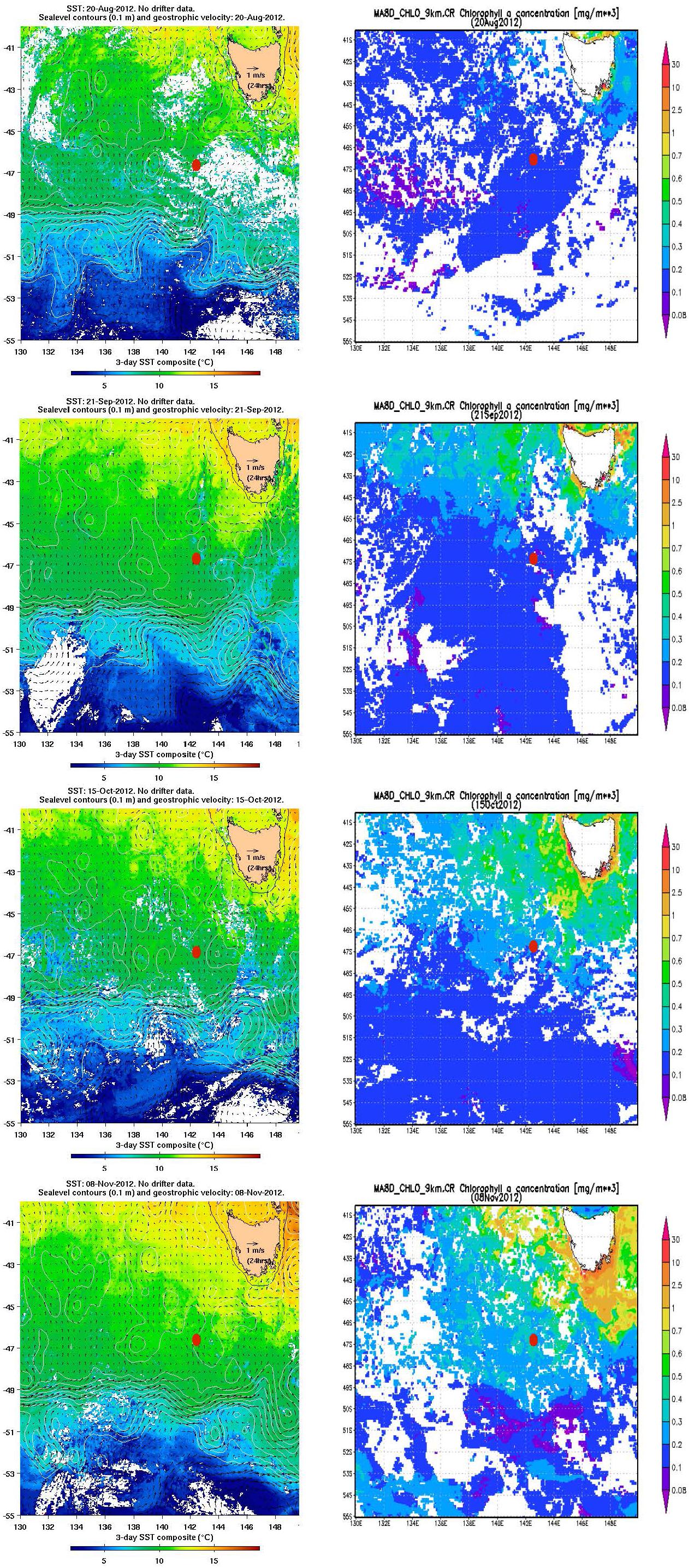
Figure 1. Maps of sea surface temperature (SST) and surface currents (left panels), and surface chlorophyll (Chla) (right panels) at approximately monthly intervals. The specific dates (20 August, 21 September, 15 October, and 8 November 2012) were selected for image quality (cloud cover precluded any clear images in December). The SOTS site is indicated by the red dots. In the SST images (left panels), the black line around Tasmania indicates the 200 m depth contour. Images produced by the IMOS Ocean Currents Facility (www.imos.org.au).
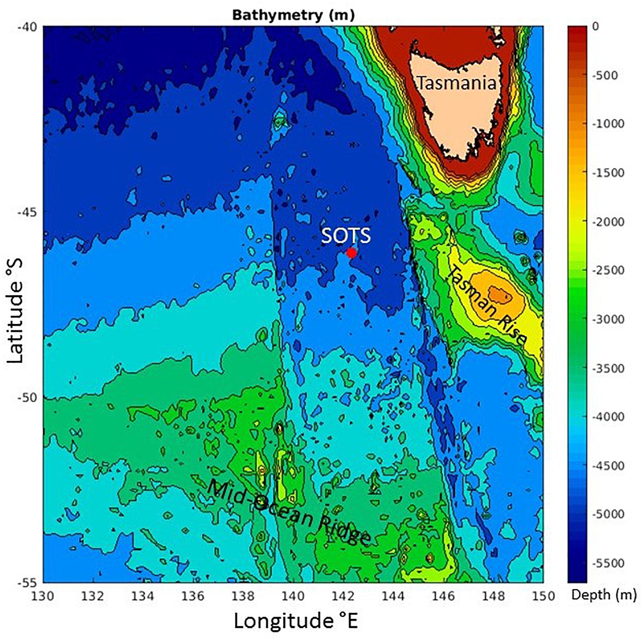
Figure 2. Bathymetric map of seafloor features near the Southern Ocean Time Series (SOTS). Image produced by the IMOS Ocean Currents Facility (www.imos.org.au).
Seasonally, SOTS exhibits deep winter mixing (to more than 500 m) accompanying SAMW formation, followed by spring stratification to yield mixed layers of ∼60–100 m depth that persist until autumn and are maintained by persistently high winds of ∼10 m s–1 and waves of ∼5 m significant height (Rintoul and Trull, 2001; Weeding and Trull, 2014). Seasonal chlorophyll accumulation is low (typically less than 0.6 μg L–1) and almost always homogeneously distributed through the mixed layer without a subsurface chlorophyll maximum, in contrast to conditions south of the Subantarctic Front (Parslow et al., 2001; Bowie et al., 2011b). Mixed layer oxygen and nitrate budgets suggest NCP is approximately 3–6 mol C m–2 year–1 (Lourey and Trull, 2001; Weeding and Trull, 2014; Cassar et al., 2015) and sinking POC export to depth as estimated from deep ocean sediment traps (deployed over full annual cycles at nominal depths of 1000, 2000, and 3800 m in the 4500 m deep water column) varies from values as low 0.13 mol POC m–2 year–1, i.e., equivalent to the global median value of ∼1 g POC m–2 year–1 (Trull et al., 2001a) to ∼10 times higher (unpublished SOTS data available on-line via IMOS), and specifically for the year examined here was ∼ 0.5 mol POC m–2 year–1 (as presented below). Shallow short-term free-drifting sediment trap deployments and 234Th surface water deficits measurements, both carried out in March 2007, suggest export production rates of 3–6 mmol POC m–2 day–1 from traps (Ebersbach et al., 2011) to 12 mmol POC m–2 day–1 from 234Th (Jacquet et al., 2011) and assuming these rates apply for the spring, summer, and autumn 9 months suggests export of 0.8 to 3.2 mol C m–2 year–1, i.e., at the lower range of the mixed layer gas and nutrient budget estimates.
As is typical of the SAZ (Lourey and Trull, 2001), nitrate remains high year round, but is accompanied by depletion of silicate to below 1 μmol L–1 (Bowie et al., 2011a, b; Eriksen et al., 2018). Iron limitation appears to be the major control on productivity (Sedwick et al., 1997, 1999; Bowie et al., 2009; Cassar et al., 2011). The phytoplankton community is diverse, with major contributions from diatoms, haptophytes, and flagellates (Kopczynska et al., 2001; de Salas et al., 2011; Cassar et al., 2015; Eriksen et al., 2018). Export fluxes to deep sediment traps are dominated by carbonates (Trull et al., 2001b) derived approximately equally from coccolithophore phytoplankton and foraminifera zooplankton (King and Howard, 2003) with significant additional contributions of biogenic silicates from diatoms (Rigual-Hernández et al., 2015) but negligible lithogenic materials.
SOTS Automated Observatory Platforms
SOTS has been based around three annually serviced moorings: (i) the Southern Ocean Flux Station (SOFS) which has a large surface float equipped with a tower and provides meteorological measurements, (ii) the Pulse biogeochemistry mooring which elastically suspends a large instrument package at 30 m depth to measure biogeochemical properties and also collects water samples, and (iii) the SAZ sediment trap mooring which collects sinking particles using conical sediment traps (Parflux-21, McLane Inc., Falmouth, MA, United States) at nominal depths of 1000, 2000, and 3800 m, and has co-located current meters. The SOFS and Pulse moorings also have temperature, salinity, and oxygen sensors distributed along their mooring lines, and the SOFS mooring supports a seawater pCO2 system in its surface float and a multi-frequency acoustic water column profiler at 30 m depth. The mooring deployments are numbered sequentially. For the July to December 2012 period studied here, the data were from SOFS-3, Pulse-9, and SAZ-15. In later years, from 2016 onward, the Pulse and SOFS capabilities were combined into a single platform.
All three platforms and most associated sensors have been described in detail previously (Trull et al., 2010; Schulz et al., 2011, 2012; Weeding and Trull, 2014; Shadwick et al., 2015). These references provide methodological details for determinations of salinity, temperature, and mixed layer depth (selected as the shallowest depth from 3 algorithms based on a temperature threshold of 0.3°C, a maximum temperature gradient, and a temperature gradient threshold of 0.005°C m–1) from sensors distributed along the Pulse and SOFS mooring lines (Weeding and Trull, 2014), heat fluxes from the SOFS mooring (Schulz et al., 2012), wave heights from accelerometers on both the Pulse and SOFS platforms (Schulz et al., 2011), and mass and POC (and other component) fluxes from the SAZ sediment traps (Trull et al., 2001b).
Automated Nutrient Sample Collections and uv-Spectrometric Nitrate Analyses
In addition to the sensor observations, autonomous samplers are used at SOTS. Specifically, the Pulse instrument pack is built around a water sampler that collects 48 × 500 mL water samples (RAS-500, McLane Inc., Falmouth, MA, United States), mounted inside a protective black plastic shroud to exclude light (Pender et al., 2010; Trull et al., 2010). The water samples were collected from a copper-screened inlet outside the shroud, in pairs, to yield approximately fortnightly resolution over the annual deployment. Nitrate and silicic acid concentrations were determined on water samples collected into 500 mL Tedlar polymer bags pre-filled with mercuric chloride to achieve a final poison concentration of 80 μM. The poisoned samples were analyzed using a continuous segmented-flow multi-channel spectrometer (Lachat, Inc.) against gravimetric seawater standards following WOCE protocols in the CSIRO Hydrochemistry Facility. Precision was ∼2% for silicate and 1% for nitrate. Comparison of nutrients to ship collected water samples suggest no biases; additional details of the processing of the RAS-500 samples are available, including protocols for phytoplankton identification from the second sample in each pair (Eriksen et al., 2018). Nitrate was also measured using a ISUS UV-spectrometric sensor (Satlantic, Inc.) operated with default factory settings and nitrate calculated using separate temperature and salinity measurements from the SBE16+ CTD following published methods (Sakamoto et al., 2009).
Chlorophyll Estimates From Fluorescence
In situ estimates of chlorophyll were obtained from measurements of chlorophyll fluorescence (stimulation at 470 nm, emission at 695 nm) using a downward facing fluorometer with a shutter (FLNTUS, Wetlabs Inc., Philomath, OR, United States) mounted on a copper plate to further inhibit bio-fouling beneath the large shrouded RAS instrument package at 30 m depth on the Pulse mooring. Sampling occurred once per hour, consisting of 5 packets of 31 flashes. Calibration prior to the deployment in February 2011 was done by the manufacturer against fluorescent solutions to determine the linear response sensitivity, with conversion to chlorophyll units based on a Thalassiosira weissflogii phytoplankton culture. Characterization of the response after the deployment in March 2016 at CSIRO using a 5-point fluorescein dilution sequence in deionized water (0 to 210 μg L−1) suggested a 7.5% decrease in sensitivity, and a dark count increase of 0.8%. Because these were within the manufacturer specified precision of 10%, we made no temporal drift correction and used the February 2011 manufacturer calibration. We found no evidence for bio-fouling during this winter through spring deployment, in either the conditions of the instruments on recovery (free of exterior surface films, but with sparse attachments of gooseneck barnacles to crevices in the shroud) or the data. In particular, the FLNTUS 700 nm backscatter channel did not exhibit high values (above 2000 m–1) that we have found are a good indicator of biofouling (Figure 3).
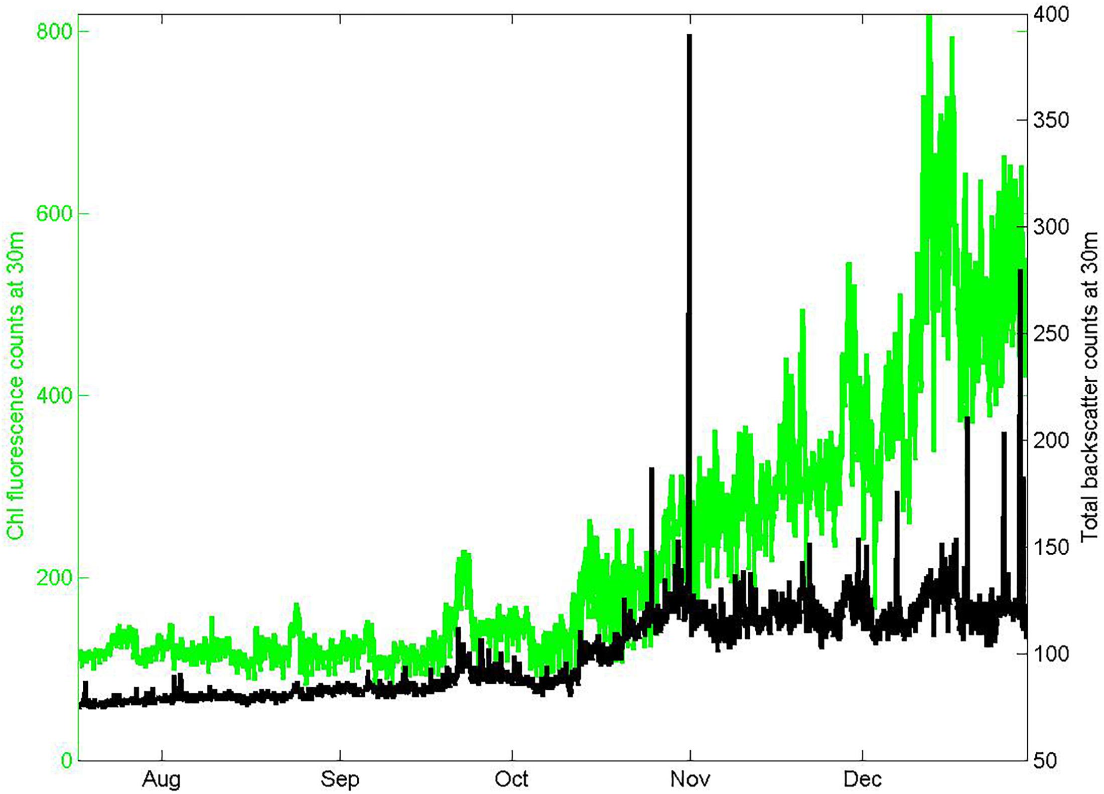
Figure 3. Seasonal records of chlorophyll fluorescence and total red light (700 nm) backscatter from the FLNTUS instrument deployed at 30 m depth on the Pulse-9 mooring. The low values of backscatter and absence of spikes are consistent with negligible bio-fouling.
Use of the manufacturer’s fluorescence calibration does not address the significant variations in fluorescence per quantity of chlorophyll that occur among different phytoplankton taxa (Proctor and Roesler, 2010). We do not have paired night time surface water moored fluorometer and pigment analyses at the SOTS site for 2012, but limited subsequent work in March 2015 (4 samples) and March 2016 (2 samples) suggests the manufacturer’s calibration over-estimates SOTS regional chlorophyll values by a factor of 2.31 ± 0.35 (unpublished data), and we have adjusted our chlorophyll estimates on this basis. This is less than the average over-estimation factor of 4 which we previously used for SOTS fluorometer results (Eriksen et al., 2018), based on comparison of radiometric and fluorescence estimates from autonomous profiling floats for the Indian sector of the Southern Ocean (Roesler et al., 2017). Clearly, these levels of characterization are insufficient to fully calibrate the fluorescence signal over the seasonal cycle. For this reason, we consider our estimates of chlorophyll concentrations as indicative only and focus our interpretation on large seasonal variations, rather than the absolute values.
Insolation and Light Attenuation
Photosynthetically active radiation (PAR) was measured in the air on the Pulse surface float using a spherical detector (MDS-MkVl, Alec Electronics Inc., Kobe, Japan), and in the ocean at the top of the RAS instrument with an upward-facing copper-shuttered planar detector (EcoPAR, Wetlabs Inc., Philomath, OR, United States). For both instruments we relied on the manufacturers’ calibrations. Quality control was assessed using syntax, range, and climatology tests following a QARTOD approach suggesting precision to a few percent but accuracies of only ∼20% (Harley et al., 2019). Therefore, as with the fluorescence chlorophyll values, we focus on large seasonal changes.
Net Community Production From Dissolved Gas Measurements
The Pulse instrument pack includes a CTD (SBE16, Seabird Inc., Seattle WA, United States) that logs two oxygen sensors (SBE 43 electrode on a pumped circuit and Aanderaa 3835 optode (Bergen, Norway) mounted to protrude into the sea beneath the shroud) and a gas tension device (GTD, Pro-Oceanus, Inc., Bridgewater, Nova Scotia, Canada). Estimation of NCP from these oxygen and total gas tension measurements on the Pulse mooring coupled with winds and atmospheric pressure data from the SOFS mooring follows the approach of Emerson et al. (2008) as used previously for SOTS observations from the 2010–2011 season (Weeding and Trull, 2014). There are many steps in this method. To provide perspective on their importance for our 2012 period we show intermediate results in Figure 4. The top panel (Figure 4A) shows the estimate of N2 saturation as derived from the gas tension device, used as a constraint on the thermal contribution to O2 saturation (Figure 4B). This allows the sum of diffusive and bubble injection contributions to the mixed layer oxygen budget to be determined from bulk air-sea gas exchange parameterizations, yielding the net biological O2 for the surface mixed layer to be obtained as a residual (Figure 4C). This budget uses the conventional assumption of negligible entrainment of oxygen poor subsurface waters from below the mixed layer, as is also generally applied to O2/Ar based NCP estimates (Cassar et al., 2007; Reuer et al., 2007; Castro-Morales et al., 2013). Unfortunately, that is a very poor assumption in the SAZ in winter when mixed layers deepen and in spring when mixed layer depth variability is large. Including entrainment estimated from mixed layer depth variations and oxygen depth profiles greatly increases the NCP estimates (Figure 4D). Thus uncertainty in the extent of entrainment dominates the NCP uncertainty estimates (Weeding and Trull, 2014), and also means that their seasonal timing is not fully independent of the stratification observations.
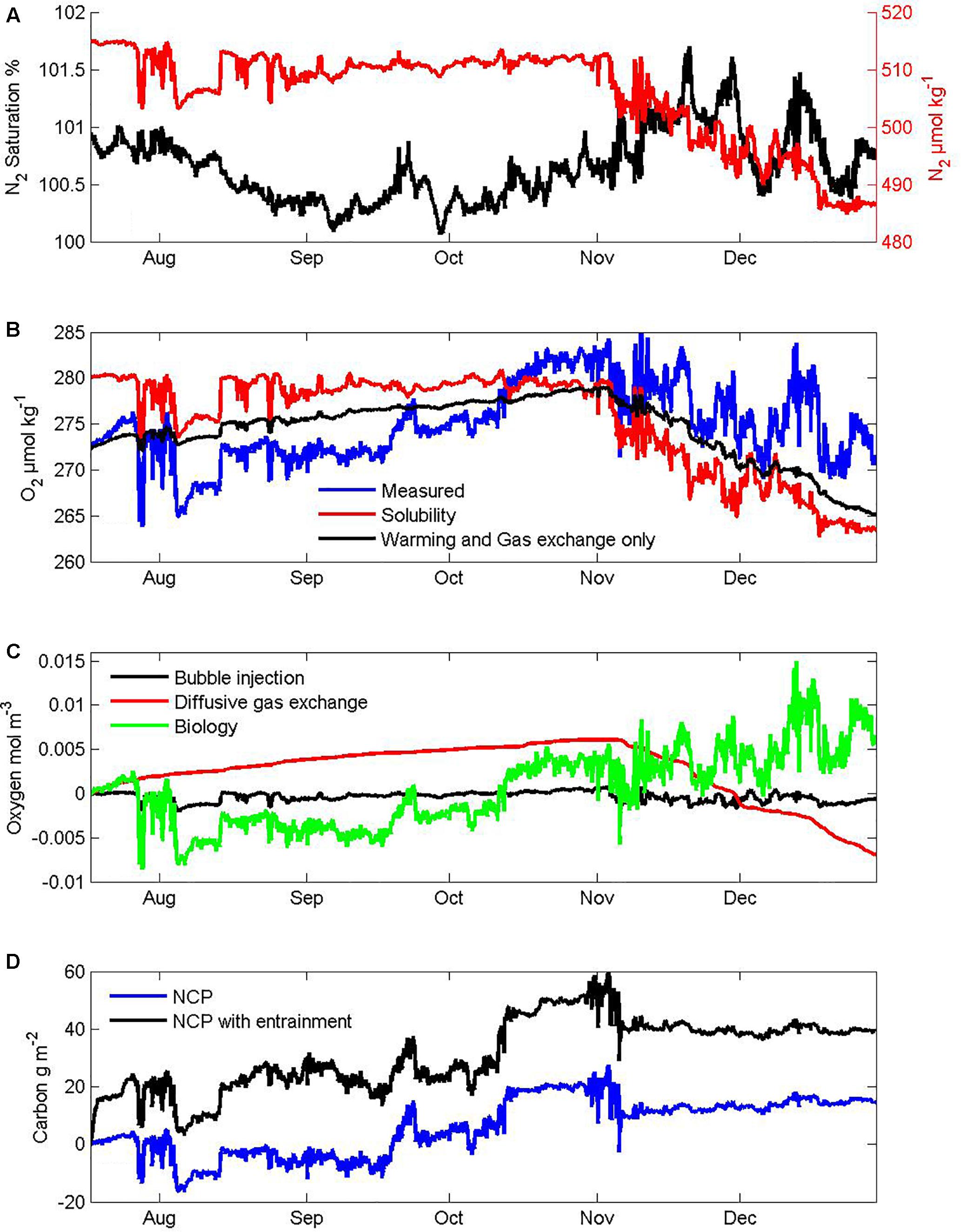
Figure 4. Intermediate steps in the derivation of net community production (NCP) from dissolved gas measurements: (A) N2 gas concentration and saturation state, (B) measured O2 concentration compared to its solubility and an expected seasonal cycle based on warming and gas exchange. Note the transition from undersaturation in winter when oxygen poor subsurface SAMW is entrained and ventilated, to supersaturation in summer that exceeds expectations from warming and gas exchange and thus indicates biological production. (C) partitioning of the oxygen inputs into contributions from diffusive gas exchange, bubble injection components, and biological processes assuming no entrainment into the mixed layer. Note the small amount of net respiration in winter and larger net production in summer. (D) cumulative net community production with and without accounting for entrainment.
Zooplankton and Higher Trophic Levels From Active Acoustics
A four-frequency (38, 125, 200, and 455 kHz) acoustic backscatter instrument (AZFP, ASL Environmental Sciences, Inc., Victoria, BC, Canada) mounted in a downward-looking configuration at 30 m depth on the SOFS platform was used to provide depth resolved estimates of the volume scattering function (Sv) as a proxy for zooplankton abundances. No evaluation of target strengths or numbers was carried out, and thus no attempt at classification of the organisms. The battery power limited sampling to a burst of 20 sound pulses every 30 min. This was just sufficient to resolve diel migration of the bulk population, but not to trace migration of individual targets. Calculation of Sv followed the procedures outlined in Deines (1999) using the beam spreading, sensitivity, and noise background recommendations from the manufacturer. Based on calibrations at 19°C versus a reference hydrophone at 1 m range and a target sphere at 4.4 m range, the manufacturer estimates an overall accuracy of ±2 dB. In producing water column maps of Sv we have retained only those Sv values more than 6 dB above the depth varying noise background. Emission off the back of the instrument and its reflection from the surface ∼30 m above produces artifacts of high scatter at ∼60 m depth, which were removed from the Sv time series.
Satellite Observations
The satellite SST observations and altimetry based estimates of currents (Figure 1) were produced by CSIRO and provided by the Australian Integrated Marine Observing System Ocean Currents Facility (technical details are available on-line: oceancurrent.imos.org.au/sourcedata/). In brief, the geostrophic currents are derived from radar altimetry using observations merged from multiple satellites, as provided by the Radar Altimetry Data Service (rads.tudelft.nl/rads/rads.shtml). The SST images are based on the L3U product from Group for High Resolution Sea Surface Temperature. The SST time series shown in Figure 5 are weekly mean values for the region 46–48°S, 140.5–142.5°E based on the NOAA optimal interpolation of in situ and satellite observations, as described and available on-line: www.esrl.noaa.gov/psd/data/gridded/data.noaa.oisst.v2.html.
Figure 5. Seasonal physical evolution of SOTS surface waters: (A) temperature and salinity in the mixed layer at 30 m depth, and an envelope of maximum and minimum satellite SST, (B) cumulative downwards heat flux and mixed layer depth, (C) wind speed and wind stress (hourly data and 8 day smoothing), (D) significant wave height (hourly data and 8 day smoothing).
The images of satellite surface chlorophyll (SChl) concentrations shown in Figure 1 are based on the MODIS Aqua, 8-day, 9 km product retrieved from the NASA Giovanni interface (Acker and Leptoukh, 2007). This provides for easy comparison to other regions of the global ocean. Comparison to pigment analyses suggests it underestimates Chl south of Australia by an average factor of 1.74 (mode of 95% range from 0.4 to 4) (Johnson et al., 2013) and accordingly we have multiplied the SChl values by this factor for comparison to the SOTS fluorescence and PAR based chlorophyll estimates in Figure 6.
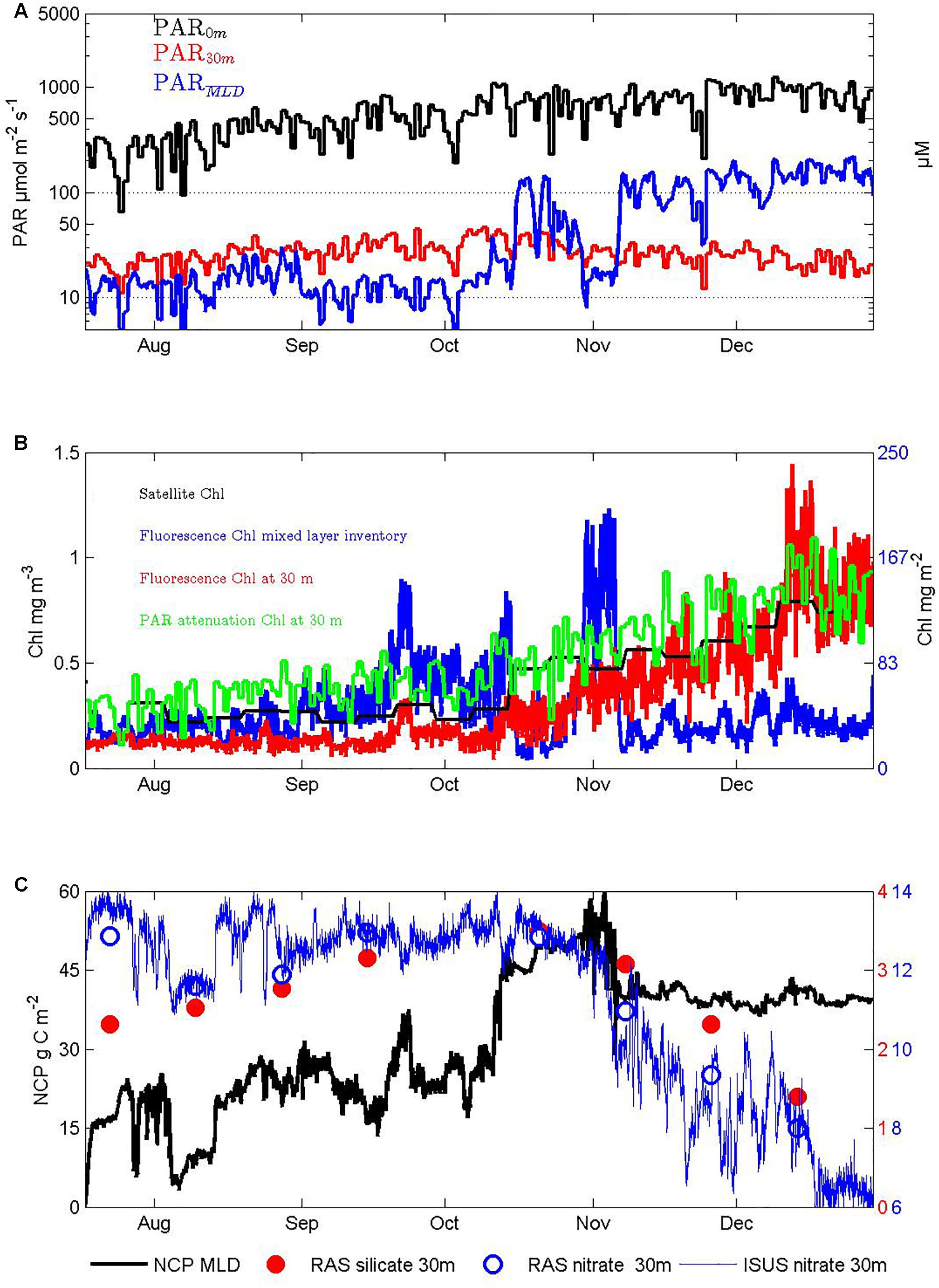
Figure 6. Seasonal response of autotrophs and their impacts on nutrients: (A) PAR at the surface, 30 m depth, and averaged over the surface mixed layer depth using the attenuation observed between 0 and 30 m depth, (B) chlorophyll estimates from satellite ocean color, PAR attenuation, the fluorometer at 30 m depth, and its integration to the mixed layer depth, (C) nitrate and silicate concentrations in the surface mixed layer at 30 m depth from the RAS water sampler, nitrate from the ISUS UV-spectrometer, and cumulative NCP from the O2-optode/N2-gas-tension-device mixed layer oxygen budget technique, after accounting for entrainment.
Results and Discussion
We focus on the timing of physical, biogeochemical, and biological events over the transition from austral winter to summer, from late July to end December 2012. We first discuss the seasonal evolution of the water column structure, then the lower trophic levels (macro-nutrients and phytoplankton), and finally zooplankton abundances and sinking particle export.
Stability and Seasonality of the Physical Environment
In general, the temporal variations in physical conditions in the SAZ were small. Salinity variations were <0.4 and seasonal warming less than 3.5°C (Figure 5A). These are typical results, as also revealed in decadal SST records (Trull et al., 2001b) and repeat WOCE/CLIVAR hydrography along 140°E south of Tasmania (Trull et al., 2001b). Winds were high on average, near 10 m s–1 (20 knots), modulated mainly on the ∼5–10 day timescales of the passage of circumpolar low pressure weather systems, with lesser seasonal variation (Figure 5C). There was a small ∼20% decrease in average wind speed in spring compared to winter, but no significant change in wind stress because the spring weather systems have higher peak wind speeds that compensate via the quadratic relationship between speed and stress. Wave contributions were also rather invariant seasonally (Figure 5D). Thus, local dynamical forcing of mixed layer depth had little seasonality, yet mixed layer depths showed extreme variation between 450 m in winter and 50 m in summer (Figure 5B), and can reach 600m in some years, as a result of both local heat fluxes (Figure 5B; Schulz et al., 2012) and Ekman transport of colder waters northward (Rintoul and Trull, 2001; Rintoul and England, 2002). Heat flux was out of the ocean until approximately 9 September (Figure 5B), and temperatures remained very close to their winter minimum of 9.1°C until the second week of October, when the first shallowing of the mixed layer began achieving depths of <100 m.
The shallow seasonal stratification was interrupted in late October when a mixed layer >400 m was again observed, but this was most likely advective in nature, rather than the result of local surface forced convection or mixing. This conclusion is based on modeling of the upper 500 m of the ocean with the Price, Weller and Pinkel one-dimensional upper ocean model (Price et al., 1986) using mooring observations for the initial ocean structure, which verified that the observed surface fluxes were insufficient to produce such a deep mixed layer. In the model this required the latent and sensible heat flux loss and wind stresses to be increased to 300 Wm–2, 200 Wm–2 and 1 Nm–2, respectively, for the two-week period, which far exceeded those observed during the November 2012 period (although equivalent fluxes have been observed in extreme winter-time cooling events when cool and dry air masses pass over the site (Schulz et al., 2012).
Seasonal Light Availability and Autotroph Responses
Daily averages of the light available for photosynthesis (PAR) measured at the surface and in the mixed layer at 30 m depth show that throughout winter these measures track each other and both slowly increase (Figure 6A). Then, from mid-October onward, while the surface PAR continues to rise, the 30 m PAR levels begin to decrease indicating additional attenuation by increasing biomass.
Exponential attenuation coefficients calculated from daily daytime average PAR values at these two depths increased seasonally from 0.08 to 0.13 m–1, i.e., even in winter there are sufficient absorbers to approximately double attenuation above that of pure seawater. The daytime PAR level averaged over the mixed layer provides one measure of light availability to fuel autotroph growth and ranged 10-fold from ∼20 to ∼200 μmol m–2 s–1 from winter into summer (Figure 6A), with primary control by mixed layer depth and only secondary influence from increasing attenuation (i.e., self-shading), which reduced mixed layer summer daytime average PAR by at most 40% (not shown).
Autotroph seasonal abundance estimates are shown in Figure 6B. Satellite Chl estimates increased ∼ 3-fold from 0.25 to 0.75 μg L–1. Similar estimates were obtained from the depth attenuation of PAR using a model that assumes it derives solely from water and chlorophyll (Morel and Maritorena, 2001). Our local calibration of fluorescence from limited pigment analyses on two voyages in autumn (see section “Materials and Methods”) agreed with these estimates in summer, but suggested lower biomass in winter, possibly as a result of lower fluorescence yield in winter when iron sufficiency is higher (Behrenfeld et al., 2009; Schallenberg et al., unpublished). Most importantly for the assessment of overall productivity, the mixed layer inventory of chlorophyll biomass showed much less seasonality, with significant inventories throughout winter and highest values in spring before stratification developed. This result adds to other recent evidence, from autonomous profiling floats equipped with fluorometers and optical back scatter sensors in both northern and southern high latitude seas (Grenier et al., 2015; Lacour et al., 2017), that satellite and in situ surface measurements are poor guides to total biomass levels, especially in winter. Biomass production in winter is also indicated by our O2/N2 based NCP estimates (Figure 6C) and by mid-winter increases in the ratio of chlorophyll fluorescence to 700 nm optical backscatter (Schallenberg et al., unpublished). Because the mean daytime light levels in the deep mixed layers in winter are quite low (∼10 μmol m–2 s–1 equating to ∼1 μmol m–2 d–1) and thus likely to be insufficient to drive production even in winter when Fe levels increase (Blain et al., 2013), it seems likely that the production occurs near the surface in periods in which the actual mixing depth is shallower than our temperature derived mixed layer depth estimates (Lindemann and St. John, 2014).
The seasonal increases in chlorophyll fluorescence in the in situ sensor record (red line in Figure 6B) included interesting shorter duration variations, such as the small peak in late September, rapid rise followed by a plateau in mid-October, narrow peak in late November, and stronger and longer peak in the first third of December. These events could arise in a multitude of ways, including resupply of iron from aerosols or deeper mixing (whether or not captured by the imperfect lens of mixed layer depth), changes in fluorescence per unit cell in response to light level variations from cloudiness or mixing or both, or the passage of parcels of water with differing autotrophic to heterotrophic activities resulting from their over-wintering histories. Their interpretation is well beyond the scope of this paper, and the complexities of separating Eulerian and Lagrangian contributions suggests progress is likely to require a statistical approach applied to the growing multi-annual records at SOTS. In this paper, we remain focused on the broad seasonal variations, and note that examination of 6 years of fluorescence records confirms that the overall seasonality described here is persistent (Schallenberg et al., unpublished).
The estimated magnitude of NCP in winter from the O2/N2 technique is very much controlled by the estimated entrainment of low oxygen deep waters, a difficult quantity to constrain (see section “Materials and Methods” and Figure 4). During the period of July to early October when mixed layers were still deepening the inferred cumulative NCP was ∼20 g m–2 (Figure 6C) equating to ∼50 mg m–3 over the 400 m deep mixed layer, and thus to ∼0.5 to 1 mg m–3 Chla, assuming phytoplankton C/Chl ratios in the range of 50 to 100 (Cloern et al., 1995); and references therein. This biomass production exceeds the winter time standing stock of ∼ 0.2 to 0.3 mg m–3 Chl (Figure 6B), and thus suggests significant transfer of carbon ∼40 to 80% of the NCP, i.e., 8 to 16 g C m–2 either to higher trophic levels or to the deep sea in the form of sinking particles (further evaluation of these possibilities is provided below in sections “Higher Trophic Level Responses” and “Pelagic-Benthic Coupling”). An alternate fate for the NCP is accumulation as dissolved organic carbon (DOC). We do not have seasonally resolved DOC data to address this, but results from the late summer SAZ Project voyage in March 1998 suggest labile surface mixed layer accumulations can reach 15–20 μmol kg–1 above deep water recalcitrant values near 45 μmol kg–1 (T. Trull and D. Davies, unpublished), equivalent over the typical 50 m summer mixed layer depth to 9–12 g C m–2, and thus 20–30% of the total seasonal NCP.
Throughout the austral winter, surface water nitrate and silicate concentrations measured in the RAS autonomous water samples (from 30 m depth) steadily increased, consistent with dominance of the system by entrainment and precluding an independent measure of NCP from nutrient drawdown. After water column stratification was complete in November, the O2/N2 mixed layer mass balance technique is more reliable (see Weeding and Trull, 2014 and Shadwick et al., 2015 and references therein for discussion), and the implied NCP between then and the end of December was relatively small ∼12 g C m–2. During this same period, the nitrate concentration decreased by ∼5 mmol m–3, equating at Redfield stoichiometry (C/N of 6.7) and integrated over the 50 m deep mixed layer to ∼20 g C m–2. This value is likely to be over-estimated because of the concomitant ∼0.1 salinity increase in this period from the summertime increase in supply of low nutrient subtropical waters. Correcting for this using typical nitrate versus salinity gradients for SAZ surface waters (Lourey and Trull, 2001) suggests nitrate consumption closer to 16 g C m–2. Given the uncertainties in the O2/N2 technique of order 50% (Weeding and Trull, 2014), these two estimates are in accord. By mid-December, the silicic acid concentration has decreased to ∼1.3 μM, and linearly extrapolating to the end of the record suggests complete depletion. This is consistent with the longer record of RAS samples from the previous year (Eriksen et al., 2018).
Higher Trophic Level Responses
The four-frequency acoustic profiler data contain a wealth of information about the abundance, water column distribution, diel cycling, and size distributions of grazing organisms and their predators. We focus on two aspects: seasonal variations in the total volume scattering above 100 m (Figure 7), and representative diel cycles from each month (Figure 8). The top 100 m volume scattering signals show similar seasonality at the three frequencies (38, 125, and 200 kHz in Figure 7; the 455 kHz signal was unable to image the full top 100 m and is not shown). Their volume scattering values decreased in July and August to minima in September and then increased 10-fold by late December. Throughout the record, volume scattering at 200 kHz was more than 10-fold greater than the lower frequency signals, consistent with dominance by smaller organisms (zooplankton) relative to larger organisms (fish). During the month of October, as water column stratification developed (Figure 7B) the lower frequency scattering increased particularly strongly. Overall, the acoustic signals suggest that the upper trophic levels disappear from surface waters in autumn and throughout the winter, and then begin to increase in early October when the mixed layer shallows and Chl concentrations increase, and thus later than the beginning of the seasonal increase in total chlorophyll inventories (Figure 6B). Unfortunately, it is not yet possible to express the acoustic signals in terms of metabolic demand, owing to insufficient information regarding the conversion of the acoustic signals into specific organism abundances (a gap we are working to fill via targeting netting and optical imaging techniques). According, we cannot yet evaluate whether the winter populations are low enough to free phytoplankton from grazing pressure and can only say that this pressure does diminish in winter.
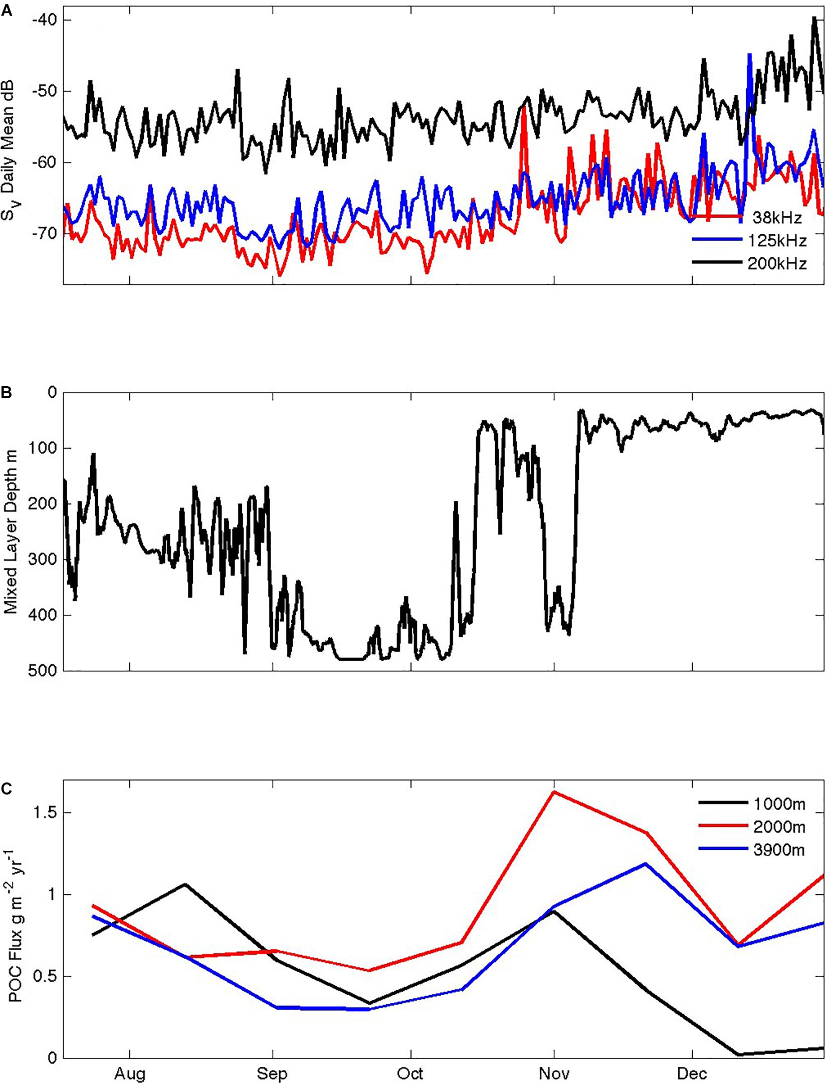
Figure 7. Seasonal responses of heterotrophs and POC fluxes to the ocean interior: (A) total volume scattering (Sv) in the top 100 m at 38, 125, and 200 kHz, (B) mixed layer depth, (C) POC fluxes at ∼1000, 2000, and 3800 m depth measured by sediment traps.
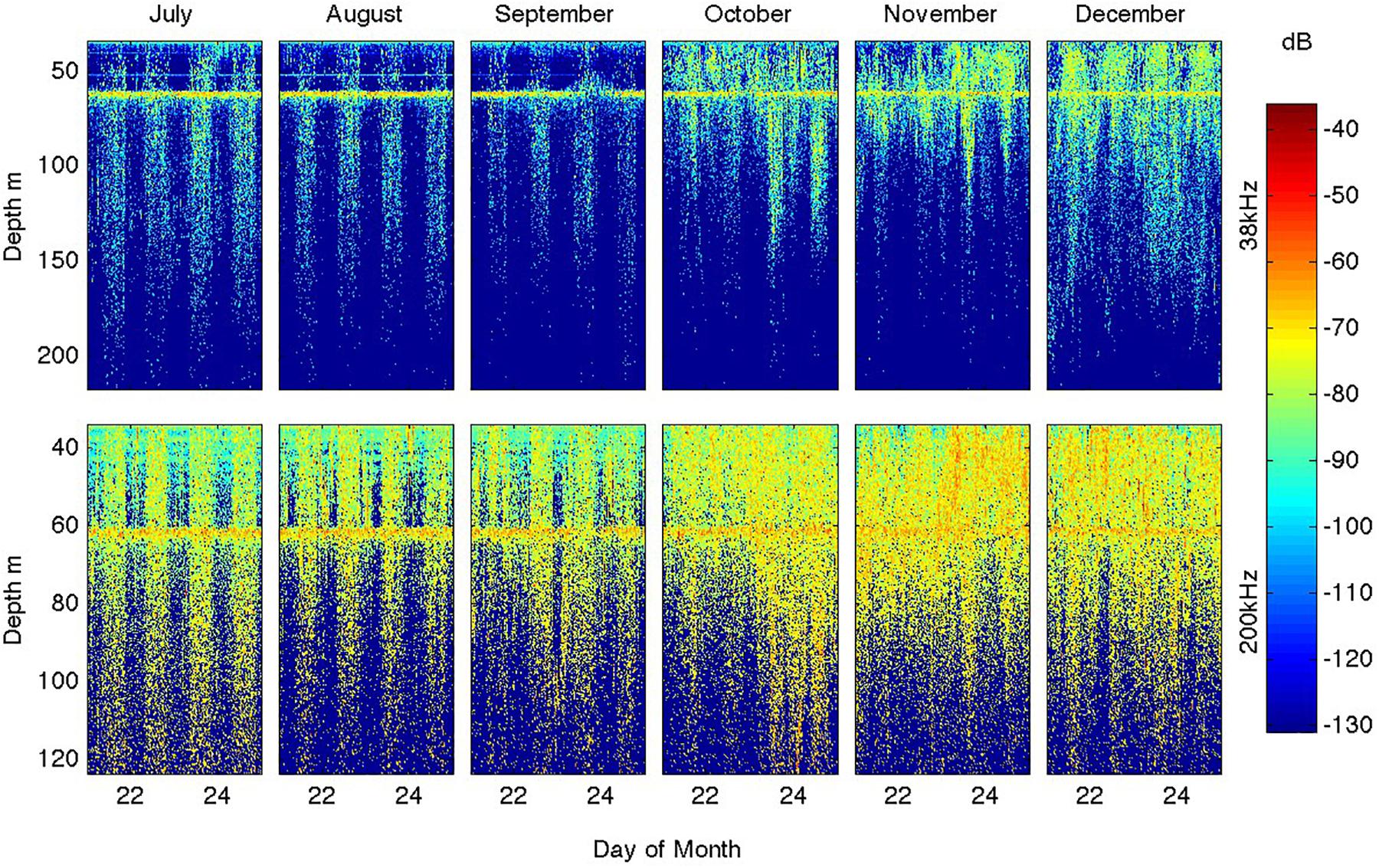
Figure 8. Seasonal evolution of heterotrophic diel migrations as revealed by the distribution of volume scattering (Sv) for 5 representative days in each of the months of July through December (left to right) at 38 and 200 kHz. The line of high-scattering at ∼60 m depth is and artifact from reflection off the surface ∼30 m above the instrument (and was removed from the total Sv time series shown in Figure 6).
In addition to the overall seasonal increases in volume scattering amplitudes, there were marked changes in their diel cycles as shown for the 38 and 200 kHz signals in Figure 8 (the 125 kHz signal showed characteristics intermediate to these frequencies). In July, August, and September the diel cycle was very sharp, with almost no scatterers present except at night and the day-night transition occurring in less than an hour (close to the 30’ acoustic sampling resolution). The night time scatterer distribution showed only weak concentration toward the surface. These characteristics applied to both the 38 and 200 kHz channels. In October, the night time increase in scatterers continued but started to be more concentrated toward the surface and was accompanied by persistence within the top ∼70 m throughout the day. This persistence was stronger for the 200 kHz channel that more effectively images small scatterers. In November, these trends intensified so that by December the 200 kHz signals showed little day-night variations within the now shallow (∼50 m) mixed layers, although night time scattering remained elevated in the 38 kHz signal. The 38 kHz signal also suggests that these larger organisms migrated to only ∼100 m depth after the water column was stratified.
Pelagic-Benthic Coupling
The coupling of upper ocean productivity to mesopelagic and benthic ecosystems is complex (Boyd and Newton, 1999; Boyd et al., 1999). In general higher productivity leads to greater particle export (Suess, 1980; Bishop, 1989), but in addition, in global comparisons, systems with strong seasonality appear to transfer a larger fraction of their production and this can be the dominant influence on POC fluxes arriving in the deep sea (Lampitt and Antia, 1997; Lutz et al., 2007). Particle export at the SOTS site as measured by deep ocean sediment traps has been previously described from an initial October to March deployment (Trull et al., 2001a) and for the slightly greater than 2 year period from July 1999 to October 2001 (Rigual-Hernández et al., 2015). These (and subsequent full annual records available on-line) show seasonal POC flux amplitudes ranging approximately 10-fold (i.e., not as peaked as in polar waters yet more strongly seasonal than in oligotrophic gyres) and also that the POC flux seasonality often includes two periods of higher flux. These are generally in spring and autumn, but sometimes merge into a broad period of higher flux that lasts throughout the summer. The timing of the spring export event varies considerably inter-annually. In the 1999–2000 year it began in July, reached a maximum in late October and was followed by very low fluxes in November (as low as those of the subsequent winter). In contrast, in the 2000–2001 record the August flux was very low; the spring peak did not start until October and reached its maximum in early December. These seasonal export records are obtained at only low temporal resolution, precluding detailed evaluation of their timing relative to features in the sensor records, and are also affected by the nature of sediment trap particle collections, which show important variations derived from the limited averaging of mesoscale spatial variability, i.e., the “statistical funnel effect” (Siegel et al., 1990; Siegel and Deuser, 1997).
In the 2011–2012 year examined here, POC fluxes were moderate in August and decreased to a seasonal low in September before increasing again in October to a spring high that peaked by late November in traps at ∼1000, 2000, and 3800 m depth (Figure 7C). It is possible that the August winter export is a remnant driven by slow sinking particles left over from production in the previous summer and autumn – a possibility suggested from silicon isotope analyses of diatoms in traps in the Polar Frontal Zone further south (Closset et al., 2015). The October increase in flux which declines again by early December is more in keeping with the seasonal timing of the mixed layer chlorophyll inventory (which peaks while mixed layers are still deep in spring) than with the surface chlorophyll concentrations (which continue to rise through December; Figure 6B). However, this correlative assessment of the phasing of production, mixed layer biomass accumulation, and export to the deep sea does not address possible seasonal variations in attenuation in the intervening mesopelagic realm, and thus further work is needed to understand the full seasonal dynamics of biological carbon pump efficiency. The apparent increase of POC fluxes with depth in Figure 7 provides another cautionary note. Multi-year records (as yet unpublished but available on-line via IMOS as detailed above) exhibit this feature in some years and not in others. Under-collection at the shallowest depth as a result of greater mooring motions coupled with less-consolidated particle structures is one possible explanation (Yu et al., 2001), which we favor over the possibility of advective supply to only the deeper traps from resuspended sediments (because there is little compositional change with depth across the major measured components of POC, biogenic silica and biogenic carbonates).
CONCLUSION
The SAZ south of Australia has one of the largest annual variations in mixed layer depth in the global ocean (Rintoul and Trull, 2001), but all other physical forcing displays only low to moderate seasonal amplitudes. Surface biomass accumulations are also relatively small, rarely exceeding 0.5 μg Chl L–1 and thus much less than classical spring blooms such as those in the North Atlantic (see section “Introduction” for citations). The autonomous observations at SOTS show that the limited biomass accumulation begins in winter, well before the establishment of warming and stratification. Moreover, when integrated over the mixed layer, biomass and NCP are similar in winter and in summer and reach their maxima in spring. The low overall, and especially daytime, acoustic volume scattering signals in winter suggest that escape from grazing pressure is a likely explanation for production initiation, i.e., tropho-dynamic decoupling as envisioned by Evans and Parslow (1985) and championed by Behrenfeld (2010). Other processes may also contribute. For example, the deepening of the mixed layer in winter entrains dissolved iron from below and this may allow phytoplankton to function at lower light levels and increase their growth rates. Observations from the SOTS region suggest this will occur when mixed layers reach the deep regional ferricline near 400–600 m depth (Sedwick et al., 1997, 2008; Lannuzel et al., 2011), and thus the timing is approximately correct (although no Fe data is available from winter or the year studied here). This effect will of course operate in concert with tropho-dynamics, and thus this view of SAZ seasonality is in essence a natural analog of the “ecumenical hypothesis” for the tropho-dynamic pre-requisites necessary for a significant response to artificial iron fertilization (Morel et al., 1991). Moreover, this winter period of production is followed by a further increase in biomass as stratification develops later in spring, presumably following the tenets regarding growth rate responses as laid out by Sverdrup (1953). Thus it seems there are multiple drivers for the initiation and development of seasonal production in the SAZ, a point recently and beautifully made for the North Atlantic (Lindemann and St. John, 2014). In this context, our most important results are the extension of the assessment of seasonal production from a traditional focus on surface phytoplankton biomass to measures of its total water column inventory, level of NCP, and coupling to trophic responses. These observations show that despite the lower biomass and lack of a marked spring bloom, the productivity and transfer of organic carbon to the ocean interior in the SAZ operates at rates close to the global median of ∼1 mg C m–2 year–1 (Trull et al., 2001a) in large part because of under-recognized winter and early spring activity.
Data Availability
All data are freely available via the Australian Ocean Data Network portal: https://portal.aodn.org.au/.
Author Contributions
TT conceived the study and wrote the manuscript. PJ was the SOTS project managing engineer, and processed all the ocean sensor records. ES processed all the atmospheric sensor records and carried out the ocean mixed layer modeling. BW computed NCP from the oxygen, total gas tension, and mixed layer depth records. DD led the RAS water sample acquisition and oversaw the nutrient analyses. SB led the SAZ sediment trap sample acquisition and oversaw the particle flux analyses. All authors contributed to the refinements of the submitted manuscript, which was further improved by the constructive and insightful inputs during the formal journal review process.
Funding
Operating support for SOTS was provided from the Australian National Collaborative Research Infrastructure Strategy via the Integrated Marine Observing System Deepwater Arrays (Southern Ocean Time Series) Facility, the Australian Commonwealth Cooperative Research Centre Program via the Antarctic Climate and Ecosystems CRC, and the Australian Marine National Facility.
Conflict of Interest Statement
The authors declare that the research was conducted in the absence of any commercial or financial relationships that could be construed as a potential conflict of interest.
Acknowledgments
We thank Mark Rosenberg (ACE CRC), the CSIRO Moored Sensor Systems teams, and the crews of the RV Southern Surveyor and RV Investigator for their expertise and good cheer during long days on deck. Thanks to postdoctoral scholars Bozena Wojtasiewicz (CSIRO) and Christina Schallenberg (ACE CRC) for suggestions for evaluation and application of the PAR and fluorescence records, and to Rudy Kloser (CSIRO) for acoustic processing guidance. RAS nutrient analyses were provided by the CSIRO Hydrochemistry Facility. Sediment trap POC analyses were provided by the UTAS Central Science Laboratory. We also thank Madelaine Cahill and the IMOS Ocean Currents Facility for assistance with Figures 1, 2.
References
Acker, J. G., and Leptoukh, G. (2007). Online analysis enhances use of NASA earth science data. Eos Trans. Am. Geophys. Union 88, 14–17.
Altabet, M. A., Deuser, W. G., Honjo, S., and Stienen, C. (1991). Seasonal and depth-related changes in the source of sinking particles in the North Atlantic. Nature 354, 136–139. doi: 10.1038/354136a0
Behrenfeld, M. J. (2010). Abandoning Sverdrup’s critical depth hypothesis on phytoplankton blooms. Ecology 91, 977–989. doi: 10.1890/09-1207.1
Behrenfeld, M. J., Westberry, T. K., Boss, E. S., O’Malley, R. T., Siegel, D. A., Wiggert, J. D., et al. (2009). Satellite-detected fluorescence reveals global physiology of ocean phytoplankton. Biogeosciences 6, 779–794. doi: 10.5194/bg-6-779-2009
Bishop, J. K. B. (1989). “Regional extremes in particulate matter composition and flux: effects on the chemistry of the ocean interior,” in Dahlem Workshop Life Sciences Report - Productivity of the oceans: Present and Past, Vol. 55, eds W. H. Berger, V. S. Smetacek, and G. Wefer, (New York, NY: John Wiley and Sons), 117–138.
Blain, S., Renaut, S., Xing, X., Claustre, H., and Guinet, C. (2013). Instrumented elephant seals reveal the seasonality in chlorophyll and light-mixing regime in the iron-fertilized Southern Ocean. Geophys. Res. Lett. 40, 6368–6372. doi: 10.1002/2013GL058065
Bowie, A. R., Griffiths, F. B., Dehairs, F., and Trull, T. W. (2011a). Oceanography of the subantarctic and Polar Frontal Zones south of Australia during summer: setting for the SAZ-Sense study. Deep Sea Res. II 58, 2059–2070. doi: 10.1016/j.dsr2.2011.05.033
Bowie, A. R., Trull, T. W., and Dehairs, F. (2011b). Estimating the sensitivity of the subantarctic zone to environmental change: the SAZ-Sense project. Deep Sea Res. II 58, 2051–2058. doi: 10.1016/j.dsr2.2011.05.034
Bowie, A. R., Lannuzel, D., Remenyi, T. A., Wagener, T., Lam, P. J., Boyd, P. W., et al. (2009). Biogeochemical iron budgets of the Southern Ocean south of Australia: decoupling of iron and nutrient cycles in the subantarctic zone by the summertime supply. Glob. Biogeochem. Cycles 23:GB4034. doi: 10.1029/2009gb003500
Boyd, P. W., Crossley, A. C., DiTullio, G. R., Griffiths, F. B., Hutchins, D. A., Queguiner, B., et al. (2001). Control of phytoplankton growth by iron supply and irradiance in the subantarctic Southern Ocean: experimental results from the SAZ project. J. Geophys. Res. 106, 31573–31584.
Boyd, P. W., and Newton, P. (1999). Does planktonic community structure determine downward particulate organic carbon flux in different oceanic provinces? Deep Sea Res. I 46, 63–91. doi: 10.1016/s0967-0637(98)00066-1
Boyd, P. W., Sherry, N. D., Berges, J. A., Bishop, J. K. B., Calvert, S. E., Charette, M. A., et al. (1999). Transformations of biogenic particulates from the pelagic to the deep ocean realm. Deep Sea Res. II 46, 2761–2792. doi: 10.1016/s0967-0645(99)00083-1
Cassar, N., Bender, M. L., Barnett, B. A., Fan, S., Moxim, W. J., Levy, H 2nd, et al. (2007). The Southern Ocean biological response to aeolian iron deposition. Science 317:1067. doi: 10.1126/science.1144602
Cassar, N., DiFiore, P., Barnett, B. A., Bender, M. L., Bowie, A. R., Tilbrook, B., et al. (2011). The influence of iron and light on net community production in the Subantarctic and Polar Frontal Zones. Biogeosciences 7, 5649–5674. doi: 10.5194/bgd-7-5649-2010
Cassar, N., Wright, S. W., Thomson, P., Trull, T. W., Westwood, K. J., De Salas, M., et al. (2015). The relation of mixed-layer carbon export production to plankton community in the Southern Ocean. Glob. Biogeochem. Cycles 29, 446–462. doi: 10.1002/2014GB004936
Castro-Morales, K., Cassar, N., and Shoosmithand Kaiser, J. (2013). Biological production in the Bellingshausen Sea from oxygen-to-argon ratios and oxygen triple isotopes. Biogeosciences 10, 2273–2291. doi: 10.5194/bg-2210-2273-2013
Cloern, J. E., Grenz, C., and Vidergar-Lucas, L. (1995). An empirical model of the phytoplankton chlorophyll: carbon ratio-the conservation factor between productivity and growth rate. Limnol. Oceanogr. 40, 1313–1321. doi: 10.4319/lo.1995.40.7.1313
Closset, I., Cardinal, D., Bray, S. G., Thil, F., Djouraev, I., Rigual-Hernandez, A. S., et al. (2015). Seasonal variations, origin, and fate of settling diatoms in the Southern Ocean tracked by silicon isotope records in deep sediment traps. Glob. Biogeochem. Cycles 29, 1495–1510. doi: 10.1002/2015gb005180
Deines, K. L. (1999). “Backscatter estimation using broadband acoustic Doppler current profilers,” in Proceedings of the IEEE Sixth Working Conference on Current Measurement (San Diego, CA: IEEE), 249–253.
de Salas, M. F., Eriksen, R., Davidson, A. T., and Wright, S. W. (2011). Protistan communities in the Australian sector of the Sub-Antarctic Zone during SAZ-SENSE. Deep Sea Res. Part II Top. Stud. Oceanogr. 58, 2135–2149. doi: 10.1016/j.dsr2.2011.05.032
Ebersbach, F., Trull, T. W., Davies, D. M., and Bray, S. G. (2011). Controls on mesopelagic particle fluxes in the Sub-Antarctic and Polar Frontal Zones in the Southern Ocean south of Australia in summer-Perspectives from free-drifting sediment traps. Deep Sea Res. Part II Top. Stud. Oceanogr. 58, 2260–2276. doi: 10.1016/j.dsr2.2011.05.025
Emerson, S., Stump, C., and Nicholson, D. (2008). Net biological oxygen production in the ocean: remote in situ measurements of O2 and N2 in surface waters. Glob. Biogeochem. Cycles 22:GB3023.
Eriksen, R., Trull, T. W., Davies, D., Jansen, P., Davidson, A. T., Westwood, K., et al. (2018). Seasonal succession of phytoplankton community structure from autonomous sampling at the Australian Southern Ocean Time Series (SOTS) observatory. Mar. Ecol. Prog. Ser. 589, 13–31. doi: 10.3354/meps12420
Evans, G. T., and Parslow, J. S. (1985). A model of annual plankton cycles. Biol. Oceanogr. 3, 327–347.
Grenier, M., Della Penna, A., and Trull, T. W. (2015). Autonomous profiling float observations of the high-biomass plume downstream of the Kerguelen Plateau in the Southern Ocean. Biogeosciences 12, 2707–2735. doi: 10.5194/bg-12-2707-2015
Harley, J., Schallenberg, C., Jansen, P., and Trull, T. W. (2019). Southern Ocean Time Series (SOTS) Quality Assessment and Control Report PAR Instruments Version 1.0. Hobart, TAS: CSIRO. doi: 10.26198/5ce4a647af256
Herraiz-Borreguero, L., and Rintoul, S. R. (2011). Regional circulation and its impact on upper ocean variability south of Tasmania (Australia). Deep Sea Res. II 58, 2071–2081. doi: 10.1016/j.dsr2.2011.05.022
Jacquet, S. H. M., Lam, P. J., Trull, T. W., and Dehairs, F. (2011). Carbon export production in the Polar Front Zone and Subantarctic Zone south of Tasmania. Deep Sea Res. II 58, 2277–2292. doi: 10.1016/j.dsr2.2011.05.035
Johnson, R., Strutton, P. G., Wright, S. W., McMinn, A., and Meiners, K. M. (2013). Three improved satellite chlorophyll algorithms for the Southern Ocean. J. Geophys. Res. Oceans 118, 1–10.
King, A. L., and Howard, W. R. (2003). Planktonic foraminiferal flux seasonality in Subantarctic sediment traps: a test for paleoclimate reconstructions. Paleooceanography 18:1019.
Kopczynska, E. E., Dehairs, F., Elskens, M., and Wright, S. (2001). Phytoplankton and microzooplankton variability between the Subtropical and Polar Fronts south of Australia (SAZ’ 98): thriving under regenerative and new production in late summer. J. Geophys. Res. 106, 597–531.
Lacour, L., Ardyna, M., Stec, K., Claustre, H., Prieur, L., Poteau, A., et al. (2017). Unexpected winter phytoplankton blooms in the North Atlantic subpolar gyre. Nat. Geosci. 10, 836–839. doi: 10.1038/ngeo3035
Lampitt, R. S., and Antia, A. N. (1997). Particle flux in deep seas: regional characteristics and temporal variability. Deep Sea Res. I 44, 1377–1403. doi: 10.1016/s0967-0637(97)00020-4
Lannuzel, D., Bowie, A. R., Remenyi, T., Lam, P. J., Townsend, A. T., Ibisanmi, E., et al. (2011). Distributions of dissolved and particlulate iron in the sub-Antarctic and Polar Frontal Southern Ocean (Australian sector). Deep Sea Res. II 58, 2094–2112. doi: 10.1016/j.dsr2.2011.05.027
Legendre, L. (1990). The significance of microalgal blooms for fisheries and for the export of particulate organic carbon in oceans. J. Plankton Res. 12, 681–699. doi: 10.1093/plankt/12.4.681
Lindemann, C., and St. John, M. A. (2014). A seasonal diary of phytoplankton in the North Atlantic. Front. Mar. Sci. 1:37. doi: 10.3389/fmars.2014.00037
Lourey, M. J., and Trull, T. W. (2001). Seasonal nutrient depletion and carbon export in the Subantarctic and Polar Frontal Zones of the Southern Ocean south of Australia. J. Geophys. Res. Oceans 106, 31463–31487. doi: 10.1029/2000jc000287
Lutz, M. J., Caldeira, K., Dunbar, R. B., and Behrenfeld, M. J. (2007). Seasonal rhythms of net primary production and particulate organic carbon flux to depth describe the efficiency of biological pump global ocean. J. Geophys. Res. 112:C10011.
Mahadevan, A., and Archer, D. (2000). Modeling the impact of fronts and mesoscale circulation on the nutrient supply and biogeochemistry of the upper ocean. J. Geophys. Res. 105, 1209–1225. doi: 10.1029/1999jc900216
Mahadevan, A., D’Asaro, E., Lee, C., and Perry, M. J. (2012). Eddy-driven stratification initiates North Atlantic spring phytoplankton blooms. Science 337, 54–58. doi: 10.1126/science.1218740
Mongin, M., Matear, R. J., and Chamberlain, M. (2011). Seasonal and spatial variability of remotely sensed chlorophyll and physical fields in the SAZ-Sense region. Deep Sea Res. II 58, 2082–2093. doi: 10.1016/j.dsr2.2011.06.002
Morel, A., and Maritorena, S. (2001). Bio-optical properties of oceanic waters- a reappraisal. J. Geophys. Res. 106, 7163–7180. doi: 10.1029/2000jc000319
Morel, F. M. M., Reuter, J. G., and Price, N. M. (1991). Iron nutrition of phytoplankton and its possible importance in the ecology of ocean regions with high nutrient and low biomass. Oceanography 4, 56–61. doi: 10.5670/oceanog.1991.03
Obata, A., Ishizaka, J., and Endoh, M. (1996). Global verification of critical depth theory for phytoplankton bloom with climatological in situ temperature and satellite ocean color data. J. Geophys. Res. Oceans 101, 20657–20667. doi: 10.1029/96jc01734
Parslow, J., Boyd, P., Rintoul, S. R., and Griffiths, F. B. (2001). A persistent sub-surface chlorophyll maximum in the Polar Frontal Zone south of Australia: seasonal progression and implications for phytoplankton-light-nutrient interactions. J. Geophys. Res. 106, 31543–31557. doi: 10.1029/2000jc000322
Pender, L., Trull, T. W., Mclaughlan, D., and Lynch, T. (2010). “Pulse – a mooring for mixed layer measurements in the open ocean and extreme weather,” in Proceedings of the OCEANS 2010 IEEE Sydney Conference, Sydney, NSW.
Price, J. F., Weller, R. A., and Pinkel, R. (1986). Diurnal cycling: observations and models of the upper ocean response to diurnal heating, cooling, and wind mixing. J. Geophys. Res. 91, 8411–8427.
Proctor, C. W., and Roesler, C. S. (2010). New insights on obtaining phytoplankton concentration and composition from in situ multispectral chlorophyll fluorescence. Limnol. Oceanogr. Methods 8, 695–708. doi: 10.4319/lom.2010.8.0695
Reuer, M. K., Barnett, B. A., Bender, M. L., Falkowski, P. G., and Hendricks, M. B. (2007). New estimates of Southern Ocean biological production rates from O2/Ar ratios and the triple isotope composition of O2. Deep Sea Res. Part I Oceanogr. Res. Pap. 54, 951–974. doi: 10.1016/j.dsr.2007.02.007
Ridgeway, K. R., and Dunn, J. R. (2007). Observational evidence for a Southern Hemisphere oceanic supergyre. Geophys. Res. Lett. 34:L13612.
Rigual-Hernández, A. S., Trull, T. W., Bray, S. G., Cortina, A., and Armand, L. K. A. (2015). Latitudinal and temporal distributions of diatom populations in the pelagic waters of the Subantarctic and Polar Frontal zones of the Southern Ocean and their role in the biological pump. Biogeosciences 12, 5309–5337. doi: 10.5194/bg-12-5309-2015
Rintoul, S. R., and England, M. H. (2002). Ekman transport dominates local air–sea fluxes in driving variability of Subantarctic mode water. J. Phys. Oceanogr. 32, 1308–1321. doi: 10.1175/1520-0485(2002)032<1308:etdlas>2.0.co;2
Rintoul, S. R., and Trull, T. W. (2001). Seasonal evolution of the mixed layer in the Subantarctic Zone south of Australia. J. Geophys. Res. Oceans 106, 31447–31462. doi: 10.1029/2000jc000329
Roesler, C., Uitz, J., Claustre, H., Boss, E., Xing, X., Organelli, E., et al. (2017). Recommendations for obtaining unbiased chlorophyll estimates from in situ chlorophyll fluorometers: a global analysis of WET Labs ECO sensors. Limnol. Oceanogr. Methods 15, 572–585. doi: 10.1002/lom3.10185
Sakamoto, C. M., Johnson, K. S., and Coletti, L. J. (2009). Improved algorithm for the computation of nitrate concentrations in seawater using an in situ ultraviolet spectrophotometer. Limnol. Oceanogr. Methods 7, 132–143. doi: 10.4319/lom.2009.7.132
Sarmiento, J. L., Gruber, N., Brzezinski, M. A., and Dunne, J. P. (2004). High-latitude controls of thermocline nutrients and low latitude biological productivity. Nature 427, 56–60. doi: 10.1038/nature02127
Schulz, E. W., Grosenbaugh, M. A., Pender, L., Greenslade, D. J. M., and Trull, T. W. (2011). Mooring design using wave-state estimate from the Southern Ocean. J. Atmos. Ocean. Technol. 28, 1351–1360. doi: 10.1175/jtech-d-10-05033.1
Schulz, E. W., Josey, S. A., and Verein, R. (2012). First air-sea flux mooring measurements in the Southern Ocean. Geophys. Res. Lett. 39:L16606. doi: 10.1029/2012GL052290
Sedwick, P., Bowie, A., and Trull, T. (2008). Dissolved iron in the Australian sector of the Southern Ocean (CLIVAR SR3 section): Meridional and seasonal trends. Deep Sea Res. Part I Oceanogr. Res. Pap. 55, 911–925. doi: 10.1016/j.dsr.2008.03.011
Sedwick, P. N., DiTullio, G. R., Hutchins, D. A., Boyd, P. W., Griffiths, F. B., Crossley, A. C., et al. (1999). Limitation of algal growth by iron deficiency in the Australian Subantarctic region. Geophys. Res. Lett. 26, 2865–2868. doi: 10.1029/1998gl002284
Sedwick, P. N., Edwards, P. R., Mackey, D. J., Griffiths, F. B., and Parslow, J. S. (1997). Iron and manganese in surface waters of the Australian Subantarctic region. Deep Sea Res. I 44, 1239–1253. doi: 10.1016/s0967-0637(97)00021-6
Shadwick, E. H., Trull, T. W., Tilbrook, B., Sutton, A. J., Schulz, E., and Sabine, C. L. (2015). Seasonality of biological and physical controls on surface ocean CO2 from hourly observations at the Southern Ocean Time Series site south of Australia. Glob. Biogeochem. Cycles 29, 223–238. doi: 10.1002/2014gb004906
Siegel, D., and Deuser, W. G. (1997). Trajectories of sinking particles in the Sargasso Sea: modeling of statistical funnels above deep-ocean sediment traps. Deep Sea Res. I 44, 1519–1541. doi: 10.1016/s0967-0637(97)00028-9
Siegel, D. A., Granata, T. C., Michaels, A. F., and Dickey, T. D. (1990). Mesoscale eddy diffusion, particle sinking, and the interpretation of sediment trap data. J. Geophys. Res. 95, 5305–5311.
Sieracki, M. E., Verity, P. G., and Stoecker, D. K. (1993). Plankton community response to sequential silicate and nitrate depletion during the 1989 North Atlantic spring bloom. Deep Sea Res. Part II Top. Stud. Oceanogr. 40, 213–225. doi: 10.1016/0967-0645(93)90014-e
Sigman, D. M., and Boyle, E. A. (2000). Glacial/interglacial variations in atmospheric carbon dioxide. Nature 407, 859–869. doi: 10.1038/35038000
Suess, E. (1980). Particulate organic carbon flux in the oceans-surface productivity and oxygen utilization. Nature 288, 260–263. doi: 10.1038/288260a0
Sverdrup, H. U. (1953). On the conditions for the vernal blooming of phytoplankton. Journal du Conseil Internationale Permanente pour l’Exploration de la Mer 18, 287–295. doi: 10.1093/icesjms/18.3.287
Taylor, J. R., and Ferrari, R. (2011a). Ocean fronts trigger high latitude phytoplankton blooms. Geophys. Res. Lett. 38, 1–5. doi: 10.1029/2011GL049312
Taylor, J. R., and Ferrari, R. (2011b). Shutdown of turbulent convection as a new criterion for the onset of spring phytoplankton blooms. Limnol. Oceanogr. 56, 2293–2307. doi: 10.4319/lo.2011.56.6.2293
Thomalla, S. J., Fauchereau, N., Swart, S., and Monteiro, P. M. S. (2011). Regional scale characteristics of the seasonal cycle of chlorophyll in the Southern Ocean. Biogeosciences 8, 2849–2866. doi: 10.5194/bg-8-2849-2011
Trull, T., Bray, S. G., Manganini, S. J., Honjo, S., and Francois, R. (2001a). Moored sediment trap measurements of carbon export in the Subantarctic and Polar Frontal Zones of the Southern Ocean, south of Australia. J. Geophys. Res. 106, 31489–31509. doi: 10.1029/2000JC000308
Trull, T., Rintoul, S. R., Hadfield, M., and Abraham, E. R. (2001b). Circulation and seasonal evolution of polar waters south of Australia: Implications for iron fertilization of the Southern Ocean. Deep Sea Res. Part II Top. Stud. Oceanogr. 48, 2439–2466. doi: 10.1016/s0967-0645(01)00003-0
Trull, T., Sedwick, P. N., Griffiths, F. B., and Rintoul, S. R. (2001c). Introduction to special section: SAZ Project. J. Geophys. Res. 106, 31425–31429. doi: 10.1029/2001JC001008
Trull, T. W., Schulz, E., Bray, S. G., Pender, L., McLaughlan, D., Tilbrook, B., et al. (2010). “The Australian integrated marine observing system Southern Ocean time series facility,” in Proceedings of the OCEANS 2010 IEEE - Sydney, Sydney, NSW, doi: 10.1109/oceanssyd.2010.5603514
Weeding, B., and Trull, T. W. (2014). Hourly oxygen and total gas tension measurements at the Southern Ocean time series site reveal winter ventilation and spring net community production. J. Geophys. Res. Oceans 119, 348–358. doi: 10.1002/2013JC009302
Yoder, J. A., McClain, C. R., Feldman, G. C., and Esaias, W. E. (1993). Annual cycles of phytoplankton chlorophyll concentrations in the global ocean: a satellite view. Glob. Biogeochem. Cycles 7, 181–193. doi: 10.1029/93gb02358
Keywords: Southern Ocean, autonomous observations, time series, seasonality, productivity, export, physical-biological coupling
Citation: Trull TW, Jansen P, Schulz E, Weeding B, Davies DM and Bray SG (2019) Autonomous Multi-Trophic Observations of Productivity and Export at the Australian Southern Ocean Time Series (SOTS) Reveal Sequential Mechanisms of Physical-Biological Coupling. Front. Mar. Sci. 6:525. doi: 10.3389/fmars.2019.00525
Received: 17 April 2019; Accepted: 12 August 2019;
Published: 28 August 2019.
Edited by:
Carol Robinson, University of East Anglia, United KingdomReviewed by:
Frank Dehairs, Vrije University Brussel, BelgiumScott Doney, University of Virginia, United States
Copyright © 2019 Trull, Jansen, Schulz, Weeding, Davies and Bray. This is an open-access article distributed under the terms of the Creative Commons Attribution License (CC BY). The use, distribution or reproduction in other forums is permitted, provided the original author(s) and the copyright owner(s) are credited and that the original publication in this journal is cited, in accordance with accepted academic practice. No use, distribution or reproduction is permitted which does not comply with these terms.
*Correspondence: Thomas W. Trull, VG9tLlRydWxsQGNzaXJvLmF1