Factors Controlling the Lack of Phytoplankton Biomass in Naturally Iron Fertilized Waters Near Heard and McDonald Islands in the Southern Ocean

Introduction

Phytoplankton are responsible for more than 45% of the global primary production (Field et al., 1998) and the sequestration of 5–10 Gt of carbon per year in the ocean through the biological pump and thus play an important role in controlling the concentration of atmospheric carbon dioxide. The Southern Ocean is the largest high-nutrient low-chlorophyll (HNLC) region in the global ocean, where phytoplankton primary production is mostly controlled by the availability of iron (e.g., Martin et al., 1990) and/or light, mainly due to little surface solar irradiance, weak density stratification, and deep mixed layers (Mitchell et al., 1991). However, in some regions, e.g., downstream of islands or in coastal polynyas, surface waters are naturally fertilized by iron, relaxing the iron limitation and leading to the occurrence of extensive phytoplankton blooms in these areas. This iron supply can come from a number of different sources, including a small input from atmospheric deposition (e.g., Jickells et al., 2005; Mahowald et al., 2005), entrainment from the deep ocean during winter mixing (e.g., Blain et al., 2008; Tagliabue et al., 2014), riverine input associated with snowmelt (van der Merwe et al., 2015), melting of sea ice and icebergs (Sedwick and DiTullio, 1997), release from sediments (e.g., de Jong et al., 2012; Hatta et al., 2013), and underwater hydrothermal activity (Holmes et al., 2017 and references therein). However, due to a relatively short lifetime of bioavailable iron in the ocean (Moore and Braucher, 2008), the regions of increased primary productivity are closely associated with local sources of this micronutrient (e.g., Blain et al., 2007; Boyd et al., 2012).

The impact of iron on phytoplankton communities in HNLC regions has been well-studied over the past few decades during a number of large scale iron fertilization experiments (e.g., Boyd et al., 2000; Coale et al., 2004; Harvey et al., 2011; Smetacek et al., 2012; Martin et al., 2013). In all of the experiments one of the direct responses of the phytoplankton to the addition of iron was an up to 20-fold increase in chlorophyll-a (chl-a) concentration from the background level to concentrations reaching 3.8 mg m⁻³ (Coale et al., 2004). Usually the photosynthetic competency response, seen as an increase in the maximum quantum yield of photosystem II (F_v/F_m), was relatively quick. It was observed in the first 2–3 days (Coale et al., 2004; Peloquin et al., 2011) and sometimes even in the initial 24 h after iron addition (Boyd et al., 2000) with the magnitude of F_v/F_m exceeding 0.6 (Coale et al., 2004; Peloquin et al., 2011). However, primary production in these areas may still be affected by light limitation in cases of deep mixed layers (Gall et al., 2001). Apart from productivity, iron addition also impacts the composition of phytoplankton communities. In the experiments performed under silica—replete conditions, diatoms eventually dominated the phytoplankton community, however in the SOIREE experiment an initial increase in the relative number of nano- and picophytoplankton was observed (Boyd et al., 2000). In cases when silica was limiting, no transition to diatom domination could be observed (e.g., Coale et al., 2004; Peloquin et al., 2011).

The Australian Territory of Heard Island and McDonald Islands (HIMI), situated in the Indian sector of the Southern Ocean, is one of the most remote places on Earth. The islands were formed by plume volcanism and are the only sub-Antarctic islands which are still volcanically active. This region is known as one of the most biologically pristine areas, because it is the only major subantarctic island group which is believed to contain no species directly introduced by human activity (AAD and Director of National Parks, 2005). It is located in the northern part of the Kerguelen Plateau, which is an area known for annual formation of phytoplankton blooms mainly due to subsurface supply of iron (e.g., Blain et al., 2001) enhanced by interaction between internal tidal waves and bathymetry (Park et al., 2008). It was observed that generally in summer these blooms were dominated by diatoms, especially Thalassiothrix antarctica and Fragilariopsis kerguelensi with variability in the taxonomic composition dependent on the location over the Plateau (Armand et al., 2008). The peak chl-a concentrations, used often as biomass proxy, are usually observed in early summer (late November/December) and generally start to fade so that by late January high biomass is limited to the plateau between Kerguelen and Heard islands (Mongin et al., 2008; Schallenberg et al., 2018).

The analysis of a time series of ocean color data (OC-CCI) from 1997 to 2015 revealed that chl-a concentrations close to HIMI were much lower compared to the central Kerguelen Plateau (Figure 1). Such a pattern was also observed by Uitz et al. (2009), who found relatively low chl-a concentrations in samples collected near Heard Island. Armand et al. (2008) also found lowest average cell abundances, lowest integrated biomass over the mixed layer and generally the least diverse phytoplankton community at a station close to Heard Island compared to other stations located over the Plateau. These observations are surprising, considering underwater hydrothermal activity, a potential source of iron, has been confirmed close to McDonald Island (Lupton et al., 2017). The concentrations of dissolved iron were relatively high and above the background levels in this area. Holmes et al. (2019) observed that among all the stations sampled during the Heard Earth-Ocean-Biosphere Interactions (HEOBI) voyage, the concentrations of dissolved Fe were sufficient to support full consumption of the available nitrogen and phosphorus only in the waters directly surrounding HIMI. However, the concentrations of all macronutrients in this area were above the limiting levels.

FIGURE 1

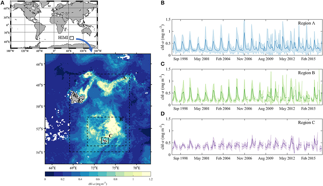
Figure 1. Variability of chlorophyll a concentration (chl-a) on the Kerguelen Plateau; (A) average chl-a in January 2013; Average chl-a between September 1997 and December 2015 in areas A, B, and C marked by dashed rectangles are presented in plots (B–D), respectively. The lines are the average chl-a and the shaded areas reflect the average ± 1 standard deviation. Pixels with no data are marked in white. All plots prepared with the use monthly OC-CCI data (http://www.esa-oceancolour-cci.org/).

The aim of this study was to investigate changes in the chl-a concentration and community structure of phytoplankton in this naturally iron-fertilized region of the Southern Ocean. The phytoplankton growth close to Heard and McDonald Islands was not limited by either dissolved iron or macronutrients, however biomass accumulation in this region was lower compared to the surrounding areas. Based on observations performed during the HEOBI voyage, we investigated a number of possible controls on biomass accumulation and changes in the phytoplankton community structure, including dilution of biomass, light limitation enhanced by the presence of resuspended sediments in the coastal shallow areas as well as the removal of phytoplankton by zooplankton grazing.

Methods

Sampling and Oceanographic Measurements

Samples were collected during the HEOBI voyage on board R/V Investigator between 8th January and 26th February 2016. Generally the measurement stations were divided into three categories; (1) stations at which only CTD casts were performed, (2) stations at which both CTD and bio-optical casts were performed, and (3) sampling stations at which both CTD and bio-optical casts were performed and water samples for laboratory analysis were collected. The sensors used at each of the CTD and bio-optical casts and types of samples collected at each of the station types are listed in Table 1. The locations of all stations analyzed in this study are given in Figure 2. During the voyage, a total of 49 CTD casts and 37 bio-optical casts were performed, and water samples were collected from 18 stations (Table 2, Figure 2). At some stations trace metal rosette (TMR) casts were performed to collect samples for determination of trace metal concentrations, including iron (Holmes et al., 2019).

TABLE 1

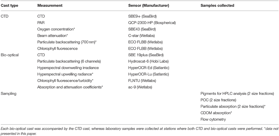
Table 1. Cast types with list of sensors used and sample types collected.

FIGURE 2

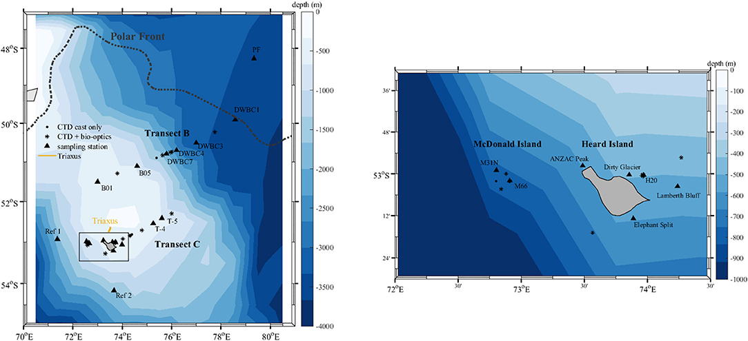
Figure 2. Geographic location of sampling stations. Colors indicate the bathymetry.

TABLE 2

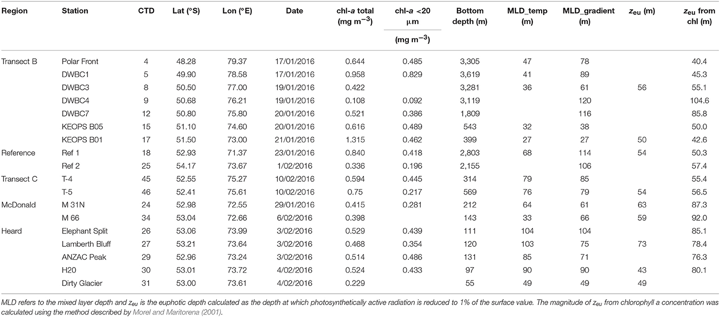
Table 2. Sampling stations during the HEOBI voyage.

The stations were further divided into five categories depending on the location; transect across the Kerguelen Plateau (transect B), transect offshore from Heard Island (transect C), McDonald Island and Heard Island (HIMI), and two off-plateau “reference” stations intended to represent HNLC oceanographic conditions in the Antarctic Circumpolar Current before contact with the Kerguelen Plateau (Figure 2). Sampling at reference station 1 revealed that it had relatively high biomass and mixed layer nutrient depletion and was likely to have formed over the plateau followed by advection off plateau (this paper; Holmes et al., 2019). For this reason, the reference station 2 was carried, which did exhibit the desired low iron, high nutrient, low biomass characteristics. This categorization of stations into regions will be used throughout the manuscript for statistical tests and analysis (including treating the reference stations as separate entities). At most sampling stations seawater was collected at three depths, but to minimize the influence of photoacclimation in the analysis of the phytoplankton community structure based on the pigment composition we only used pigment samples collected in the first optical depth, calculated as z_eu/4.6 (Gordon and McCluney, 1975), where z_eu (m) is the euphotic depth. The euphotic depth was determined using PAR profiles or fluorescence-derived chlorophyll profiles using the model of Morel and Maritorena (2001) in the case of night-time stations (Table 2). The model was only used for the open ocean stations due to high amounts of suspended sediments at stations close to HIMI.

The mixed layer depth (MLD) is a useful, though complex, concept for the evaluation of the depth of homogenization of surface derived properties downward into the water column, and for the exchange between the mixed layer and deeper waters (especially via the rate of change of the MLD as an indicator of entrainment). Here we use it primarily to estimate the average and median light levels experienced by phytoplankton and thus to compare the likelihood of light limitation among the different stations. Secondarily, we use it as an indicator of when surface forced mixing is sufficient to entrain particles resuspended from underlying sediments. Many possible MLD estimates can be calculated (for a recent review see Table 1 of Carvalho et al., 2017). Broadly speaking, these can be divided into two classes: threshold criteria which represent the depth at which properties first change significantly from surface values, and gradient criteria which determine the depth where subsurface properties change rapidly (typically either as the location of the maximum gradient, or as the first depth at which the gradient exceeds a threshold). The MLD evaluation can be done on temperature, salinity, density, or in principle any other property including biomass itself. The best choice depends on the intended subsequent use of the MLD estimate. The chosen method used often reflects a timescale, and can also provide some separation between the mixing depth to which turbulence is currently stirring the water column and the mixed depth to which past events have homogenized its properties (e.g., Brainerd and Gregg, 1995; Lacour et al., 2017, 2019).

Our two chosen MLD methods illustrate these issues. Estimating MLD using a 0.2°C decrease from surface values threshold criterion (de Boyer Montégut et al., 2004) yields relatively shallow MLD estimates (Table 2), and was equivalent to a ~0.02 kg m⁻³ density decrease (downward salinity variations were negligible). Estimating MLD using the depth of the maximum density gradient yields deeper values (Table 2). In the temporal perspective, the shallower MLD estimates reflect the extent of recent mixing, while the deeper estimates are remnants from earlier deep mixing events, often reflective of end of winter mixing. This is typical of the seasonal progression described previously for the waters of the Kerguelen plateau and its downstream biomass plume from profiling float records (Grenier et al., 2015), which reveal the abandonment of biomass below the mixed layer in response to seasonal insolation. Because of our focus on light limitation of production, we use the shallower temperature threshold MLD estimates, reflecting contemporaneous stirring, as the main criterion for comparing sites, but also comment on how the deeper maximum density gradient MLD estimates would influence our conclusions.

Pigment Measurements

High-Performance Liquid Chromatography (HPLC)

At each sampling station two 2-liter seawater samples were collected from the Niskin bottles for the size-fractionated pigment analysis. One of the samples contained all particles whereas the second one was pre-filtered through a 20 μm filter. Next, samples were filtered through 0.7 μm glass-fiber Whatman GF/F filters, frozen in liquid nitrogen and kept at −80°C until analysis. Pigments were extracted in acetone and analyzed by High-Performance Liquid Chromatography (HPLC) with a Waters-Alliance system, following the CSIRO protocol, as described by Clementson (2012). Pigments were identified by retention time and the absorption spectra from a photo-diode array detector and their concentrations were determined through peak integration performed in Empower software. The detection limit of this method for most pigments is within the range of 0.001–0.005 mg m⁻³.

Pigment-Based Phytoplankton Community Size Structure

The phytoplankton community size structure, i.e., the contribution of micro-, nano-, and picophytoplankton, was derived using the pigment-based method (Uitz et al., 2006). The method is based on seven diagnostic pigments for specific phytoplankton groups, which have been assigned to size classes based on the average size of the cells with coefficients derived using a global database of HPLC measurements. For example, fucoxanthin and peridin are used as marker pigments for diatoms and dinoflagellates, respectively, which are both classified as microphytoplankton. The contribution of each of the size classes was calculated as:

$\begin{array}{ll}{f}_{\text{micro\_HPLC}}=(1.41\text{ Fuco}+1.41\text{ Peri})/\text{wDp}& (\mathrm{1a})\end{array}$

$\begin{array}{l}{f}_{\text{nano}\_\text{HPLC}}=(1.27 19^{\prime }-\text{HF}+0.60 \text{Allo}\\ +0.35{19}^{\prime }-\text{BF})/\text{wDP}& (\mathrm{1b})\end{array}$

$\begin{array}{ll}{f}_{\text{pico\_HPLC}}=(0.86\text{ Zea}+1.01\text{ Tchl}b)/\text{wDP}& (\mathrm{1c})\end{array}$

where Fuco, Peri, 19′-HF, Allo, 19′-BF, Zea and Tchlb are concentrations of fucoxanthin, peridinin, 19′-hexanoyloxyfucoxanthin, alloxanthin, 19′-butanoyloxyfucoxanthin, zeaxanthin, and total chlorophyll b, respectively, and wDP is the weighted sum of the concentrations of the diagnostic pigments with the coefficients calculated using a global database of HPLC pigments:

$\begin{array}{l}\text{wDP}=1.41\text{ Fuco }+1.41\text{ Peri }+1.2719^{\prime }-\text{HF}+0.60\text{ Allo}\\ +0.3519^{\prime }-\text{BF}+0.86\text{ Zea}+1.01\text{ Tchl}b& (2)\end{array}$

The joint contribution of pico- and nanophytoplankton was also calculated using our size fractionated (SF) pigment data:

$\begin{array}{ll}{f}_{\text{nano\_SF}}+f_{\text{pico\_SF}}=\frac{\text{Tch}{\text{l}}_{<20\mu \text{m}}}{\text{Tch}{\text{l}}_{\text{total}}}& (\mathrm{3a})\end{array}$

$\begin{array}{ll}{f}_{\text{micro\_SF}}=1-(f_{\text{nano\_SF}}+f_{\text{pico\_SF}})& (\mathrm{3b})\end{array}$

where Tchl is total chlorophyll a concentration calculated as a sum of mono- and divinyl chlorophyll a and chlorophyllide a.

Chlorophyll-a Concentration From Fluorescence

In addition to pigment concentrations, chlorophyll-a (chl-a) fluorescence was also measured with a fluorometer (ECO, FLBBRTD-3698, WetLabs) on the CTD rosette during all casts. Another fluorometer (AQUATRACKA MKIII 11-8206-001, Chelsea) was used in the underway system allowing for measurements being taken continuously during the entire voyage. For both devices the raw counts were converted into chl-a concentration using factory-provided calibration sheets. It is worth noting that the retrievals of chl-a concentration from in situ fluorometers in the global ocean on average differ from the concentrations measured by the HPLC technique by a factor of 2, and in the Southern Ocean by a factor of 8, due to variations in the community composition of the phytoplankton assemblage (Roesler et al., 2017). Therefore, chl-a concentrations derived from fluorescence were compared to chl-a concentrations measured using the HPLC method, and the obtained relations were used to calibrate both fluorometers.

Phytoplankton fluorescence is also affected by a process known as non-photochemical quenching (NPQ), which manifests itself as a decrease in the fluorescence to chl-a concentration ratio in the surface layer during the day. Therefore, only surface and underway measurements collected at night were used for calibration of both fluorometers and taken into further analysis. When entire chl-a profiles were analyzed, the parts of the profiles with photosynthetically active radiation (PAR) higher than 20 μmol photons m⁻² s⁻¹ were discarded as being affected by NPQ.

Flow Cytometry

Samples (1 mL) were collected from the Niskin bottles, preserved with glutaraldehyde (0.1% final concentration), quick frozen in liquid nitrogen and kept deep frozen at −80°C until analysis. Samples were analyzed using flow cytometry to enumerate picophytoplankton and nanophytoplankton. Samples were thawed at 37°C, 1 μm beads (Polysciences) added as an internal standard and analyzed using a FACSVerse (Becton Dickenson) flow cytometer fitted with a 488 nm laser. To enumerate smaller picophytoplankton, acquisition was run for 3 min on a medium flow rate (~63 μL min⁻¹). To enumerate larger picophytoplankton (i.e., picoeukaryotes) and nanophytoplankton, the settings were adjusted so as to include all picoeukaryotes and nanophytoplankton, and run for 5 min on a high flow rate (111 μL min⁻¹). Each sample tube was weighed before and after flow cytometric analysis to calculate the sample volume analyzed.

Following flow cytometric analysis, picophytoplankton and nanophytoplankton groups were discriminated on the basis of red and orange auto-fluorescence of chlorophyll and the accessory pigment phycoerythrin and side-angle light scatter (SSC) and forward-angle light scatter (FSC) properties, using the flow cytometry analysis software FlowJo^®.

Photosynthetic Physiological Parameters

Phytoplankton photo-physiological parameters were estimated from continuous measurements of fluorescence induction and relaxation using a FIRe instrument (SN27; Firm/Soft-ware FIReCOM 1.1.4; Satlantic Inc.), installed in-line via opaque plumbing to the ship scientific seawater supply with a flow rate of ~0.5 L min⁻¹ through its optical cell. The FIRe technique stimulates fluorescence with a blue flash (450 nm) and measures the red-light response (680 nm). The default single turnover flash (STF) sequence was used, consisting of an initial 14 μs of dark measurements (the average of the last 11 of these are used to correct subsequent fluorescence measurements for the instrument dark current); a number of intense induction flash (~50,000 photons m⁻² s⁻¹) for a period of 80 μs (with individual flashes space 1 μs apart) during which the fluorescence yield rises to a maximum and is measured approximately every 1 μs; and a relaxation phase of 15,000 μs during which the drop in fluorescence is measured at temporally increasing intervals designed to optimize determination of its multi-exponential decay. The sequence of fluorescence yields are interpreted by fitting to the model of Kolber et al. (1998). This yields a suite of photo-physiological parameters, including the photosystem (PSII) absorption cross-section and the variable fluorescence (F_v) determined from the asymptotic rise from the dark-adapted initial fluorescence (F₀) to the saturated maximal fluorescence (F_m).

Here we focus on estimates of the quotient F_v/F_m, which provides an estimate of the quantum efficiency of photosynthetic electron transport, i.e., a measure of the effectiveness of the phytoplankton at converting light into chemical energy. F_v/F_m reaches values of ~0.67 at maximal efficiency. Lower values may indicate physiological deficiencies, often as a result of insufficiency of Fe or other nutrients (Smyth, 2004; Peloquin and Smith, 2007), although variations also occur with changes in community composition (Suggett et al., 2009). We do not address the causes of low F_v/F_m values here and only interpret values of F_v/F_m > 0.5 as indicating that those phytoplankton communities are likely to have been Fe replete. This is consistent with results for Southern Ocean phytoplankton from both laboratory mono-cultures and ocean community samples (Strzepek et al., 2012; Alderkamp et al., 2019), which have also shown that light limitation can further (but secondarily) increase F_v/F_m when Fe is replete. We use only results measured at night, to ensure accordance with the definition of F₀ as pertaining to dark-adapted cells.

Particulate Organic Carbon (POC) and Particulate Nitrogen (PN)

At each of the stations sampled for pigment analyses, duplicate samples were collected from Niskin bottles via cleaned silicon hose into pre-rinsed 2-liter sample bottles. Both samples passed through 200 μm Nitex mesh in-line 47 mm diameter pre-filters to remove zooplankton, and one of the pair also passed through 20 μm Nitex mesh to remove micro-plankton. The particulate matter in these 2-liter samples was then filtered onto 1.2 μm pore size Sterlitech 25 mm diameter silver filters, dried at 60°C under cover in a dedicated clean oven, stored and transferred to shore in sealed plastic containers. The samples were exposed to HCl to remove inorganic carbonates and then analyzed for POC and PN by high-temperature combustion at the University of Tasmania Central Sciences Laboratory against casein and sulphanilamide standards with precision of a few percent, following the methods detailed by Trull et al. (2018). Corrections in the order of 10% were made for processing blanks (based on performing shipboard protocols to filter only a few mL), and their variability is the source of our overall precision estimate of 15%.

Optical Backscattering

The particulate backscattering coefficient, b_bp, was determined at 6 wavelengths (442, 488, 550, 589, 676, 850 nm) with the use of a Hydroscat-6 (HOBILabs) as detailed in Maffione and Dana (1997). The profiles were taken down to 240 m and the data were binned into 1-m bins. The volume scattering function at chosen wavelength λ and angle θ_c, β(λ, θ_c), measured by Hydroscat-6 consists of the input of backscattering from particles β_p(λ, θ_c) and molecular scattering of light by seawater β_w(λ, θ_c). The backscattering by seawater at the sensor scattering angle (140°) and each wavelength was calculated using temperature and salinity profiles measured at the same time with the use of a SeaBird 19plus CTD following Zhang et al. (2009) with a depolarization ratio of 0.039. Then the total hemisphere particulate backscattering coefficient from particles (b_bp) was calculated as:

$\begin{array}{ll}{b}_{\text{bp}}(\lambda )=2\pi \chi \left[\beta (\lambda ,{\theta }_c)-{\beta }_w(\lambda ,{\theta }_c)\right]& (4)\end{array}$

where χ = 1.08 (Maffione and Dana, 1997) is the ratio of the total hemispheric signal to the sensor angle signal.

Due to the contamination of the signal at the surface by the presence of air bubbles the upper 5 m of data were not used in the analysis. Some backscattering profiles exhibited significant spikes which were probably associated with large particle aggregates (Briggs et al., 2011). Therefore, we used a 7-point running median followed by a running mean filter to smooth the profiles following the recommendations given by Briggs et al. (2011).

Radiometry

Profiles of hyperspectral downward irradiance were measured during the bio-optical casts using the HyperOCR radiometer (Satlantic Inc.). The measurements were taken between 350 and 800 nm with a resolution of ~3.3 nm. All measurements were dark-corrected using values measured during each profile with the internal shutter covering the sensor. For PAR, the measurements from the sensor mounted on the main CTD rosette were used in order to increase the amount of available data. After calibration all radiometric measurements were binned into 1-meter bins. The profiles were quality checked and those displaying non-realistic shape diverging from the expected exponential decrease with depth were discarded from the analysis. The euphotic depth, z_eu, was calculated as the depth at which the surface PAR is reduced by 99%. In order to calculate the diffuse light attenuation coefficients, K_d(490) and K_d(PAR), a linear function was fitted to the depth and natural logarithm of E_d(490) or PAR, respectively. K_d(490) and K_d(PAR) were calculated for the mixed layer and for specific depths in the profiles. In the first case, the linear fitting was performed in the layer from the surface down to mixed layer depth. In the latter case, data in the 20-meter layer centered on the depth of interest were used for the fitting.

Triaxus

During the voyage we also performed a short Triaxus transect (Figure 2). Triaxus is a towed vehicle gliding between surface and ~200 m that can be equipped with multiple sensors. In this study, data on temperature, salinity, PAR, particulate backscattering at 700 nm and chlorophyll-a fluorescence were collected. All data from sensors mounted on Triaxus were processed in the same manner as data from the main CTD or bio-optical package. Chlorophyll-a concentration was derived using the factory calibration, but due to the lack of any HPLC samples collected concurrently we did not perform the second step calibration. This will not affect our analysis because with this data set we were interested in the relative change of the chlorophyll-a concentration and the particulate backscattering to chlorophyll-a ratios, not their actual magnitude. All data from the Triaxus transect are available on-line (http://www.marlin.csiro.au/geonetwork/srv/eng/search#!4efe89e1-b55d-435f-bd31-dc3fbe83ab95).

Results

Phytoplankton Biomass

The total surface chlorophyll a (chl-a) concentration in the sampled region varied between 0.2 and 1.3 mg m⁻³ (Table 2, Figure 3A). Due to scarcity of HPLC samples we used the night data from the fluorometer mounted on the CTD to compare different regions indicated in Figure 2. The highest surface chl-a concentrations, calculated as the median within the upper 20 meters of the profile, were observed at transect B stations ranging between 0.17 and 1.10 mg m⁻³ with a median of 0.51 mg m⁻³. The lowest concentrations ranging from 0.17 to 0.26 mg m⁻³ with a median of 0.26 mg m⁻³ were recorded close to Heard Island. The chl-a concentration in this region was statistically different from the values observed at transect B (Kruskal-Wallis test, p = 0.002) and transect C stations (Kruskal-Wallis test, p = 0.015). A similar trend was obtained when all the underway chl-a concentration data were analyzed (Figure 3B).

FIGURE 3

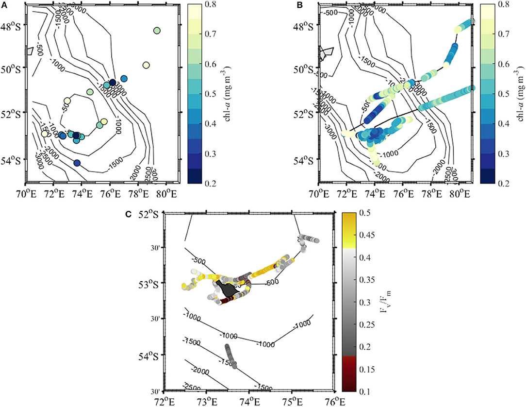
Figure 3. Concentration of chlorophyll a (chl-a) at the surface measured by (A) HPLC and (B) underway fluorometer, and (C) maximum quantum yield of photosystem II (PSII)—F_v/F_m in the vicinity of Heard and McDonald islands.

Although it has been shown that the analysis of phytoplankton spatial trends using chl-a alone has its limitations (Siegel et al., 2013) mostly because carbon to chlorophyll ratios in phytoplankton can vary within a relatively broad range, we did not see any statistically significant differences in the surface POC to chlorophyll ratios among different regions (Kruskal-Wallis test, p = 0.308) with the values ranging between 34.0 to 187.9 with median values of 77.6, 69.0, 76.9, and 94.0 for reference, transect B, transect C and Heard and McDonald Islands, respectively. The highest magnitude of the ratio (187.9) was observed to the north of Heard Island at the station (Dirty Glacier) directly affected by the glacier outflow.

The highest values of the maximum quantum yield of PSII (photosystem II), F_v/F_m, around 0.5 were found around McDonald Island, north-east of Heard Island and about half way along transect C. On the other hand the lowest values of ~0.1 were detected to the south of Heard Island and all the way down to reference station 2 (Figure 3C).

Phytoplankton Community Size Structure

At most sampling stations the phytoplankton community was dominated (>50%) by microphytoplankton (phytoplankton larger than 20 μm) with the contribution of this fraction decreasing to about 20% close to Heard and McDonald Islands (Figure 4A). The phytoplankton size structure derived using marker pigments (Equations 1, 2) overestimated the contribution of microphytoplankton, by 35.7 ± 14.5% compared to the size-fractionated chlorophyll concentration (Figure 4B). However, the pattern with the decrease of the microphytoplankton contribution in the vicinity of the islands was observed with both methods. One of the reasons for the overestimation of the pigment-derived microphytoplankton contribution was the relatively high concentration of fucoxanthin in the <20 μm fraction (Figure 4C), which may point to the abundance of diatoms smaller than 20 μm or possibly haptophytes.

FIGURE 4

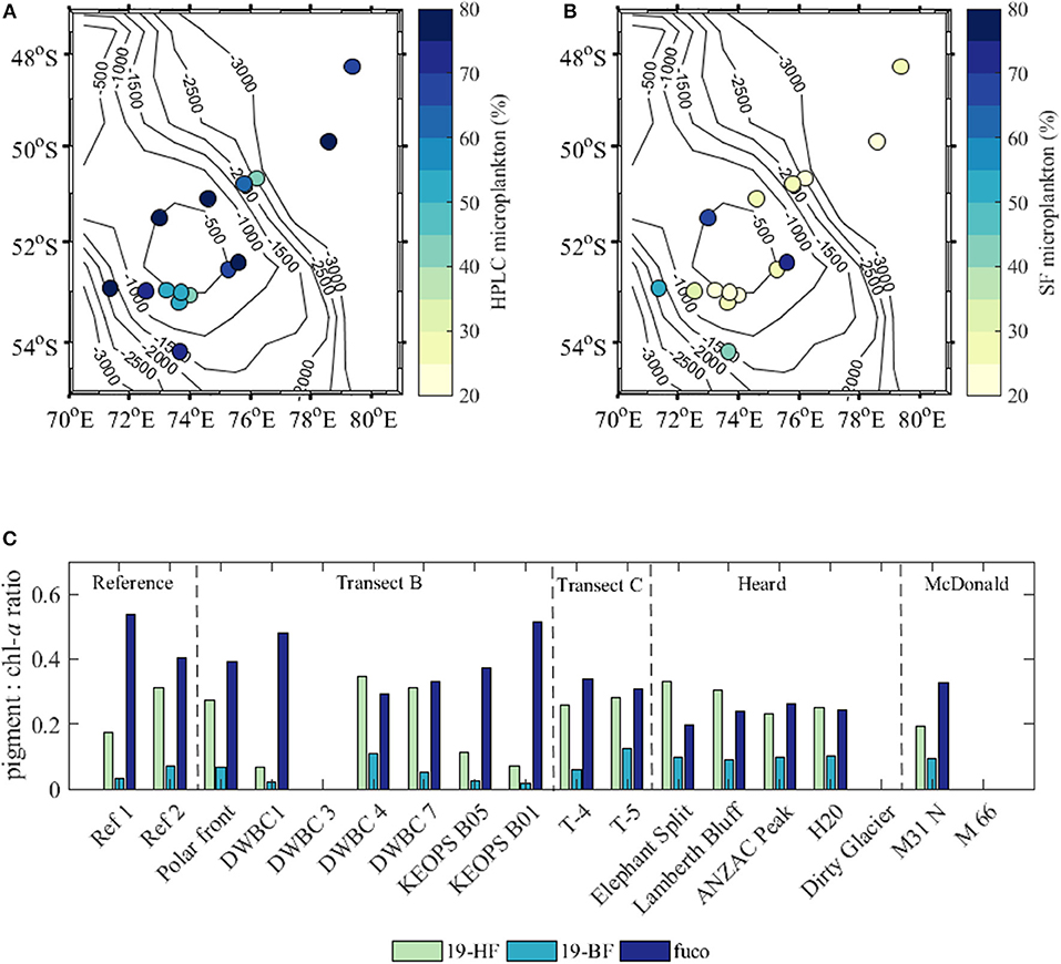
Figure 4. Contribution of microphytoplankton [as percentage (%)] to total phytoplankton biomass (A) using the Uitz et al. (2009) model based on the pigment concentration and (B) size-fractionated total chl-a data; (C) ratios of pigments 19′-hexanoyloxyfucoxanthin (19-HF), 19′-butanoyloxyfucoxanthin (19-BF), and fucoxanthin (fuco) to chlorophyll a concentration (chl-a) in the <20 μm size fraction.

In this study, the concentration of fucoxanthin relative to the chl-a concentration was higher at reference and transect B and C stations compared to Heard and McDonald Island stations, at which a high magnitude of 19′-HF and 19′-BF to chl-a was observed (Figure 4C). Peridinin, another marker pigment for microphytoplankton (Equation 1a), was only found at some transect B stations, which indicates quasi-absence of dinoflagellates at most locations within the study region.

The flow cytometric analysis distinguished three picoplankton groups (Synechococcus and two likely picoeukaryote groups (P1 and P2) and three nanoplankton groups (N1, N2, N3) (Figure 5). Relatively low cell abundances of Synechococcus occurred at the beginning of Transect B, at the station located close to the Polar Front (Figure 5A). From the Polar Front station south-west toward the Plateau and Heard Island the total number of cells and the contribution of picoplankton steadily decreased (Figure 5B). At Heard and McDonald stations the total number of phytoplankton cells, including both pico- and nanoplankton, was considerably lower than measurements conducted at Transect B stations (Figure 5C) with nanoplankton dominating (i.e., >80%) the total picoplankton and nanoplankton cell counts at all HIMI stations (Figure 5D). The N3 group was relatively more abundant at Heard Island stations and contributed up to 30% of total picoplankton plus nanoplankton cell counts (Figure 5D) compared to its marginal contribution below 5% at transect B stations (Figure 5B), but this group was absent at McDonald stations. Domination of nanoplankton as determined with flow cytometry agrees with the results of the pigment analysis.

FIGURE 5

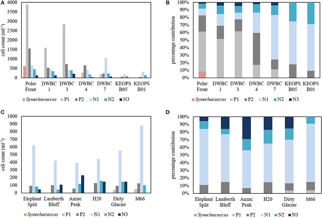
Figure 5. Variability in the pico- (Synechococcus, P1, and P2) and nanophytoplankton (N1, N2, N3) cell counts and community composition from flow cytometry measurements; (A) cell counts for all Transect B stations; (B) Percentage contribution of pico- and nanophytoplankton groups to total cell counts at stations along Transect B; (C,D) the same as (A,B) for Heard and McDonald Island stations. Note different y-axis scales for (A,C).

Discussion

The dissolved Fe and macronutrient concentrations measured in the vicinity of both Heard and McDonald Islands were sufficient to prevent limitation of phytoplankton growth in the areas where relatively low phytoplankton biomass was observed (Holmes et al., 2019). Generally, concentrations of macronutrients in the surface layer close to Heard or McDonald Islands were not statistically different from other regions (Kruskal-Wallis test, p < 0.05). Therefore, the lack of phytoplankton biomass in the surface layer in this region is surprising, especially given the observed high F_v/F_m values indicating healthy phytoplankton communities (Figure 3C; see also Methods section Photosynthetic Physiological Parameters for background on the relative impacts of iron and light limitation on Fv/Fm values). This result may be caused by a number of processes among which dilution of biomass caused by deep and lateral mixing, removal of biomass by circulation and/or zooplankton grazing and light limitation of phytoplankton growth are the most probable ones and will be discussed further.

Possible Explanations for the Low Biomass

Vertical Mixing

Low concentrations of chl-a at the surface as seen in the ocean color products (Figure 1) and our in situ samples (Figure 3) could simply be caused by the dilution of biomass due to deep mixing. However, the depth-integrated chl-a concentrations within the water column at HIMI stations were significantly lower than those observed at stations on both transects (Kruskal-Wallis test, p < 0.05). The mixed layer depth in the vicinity of the islands was in some cases extended to the seabed, especially in the case of stations located close to Heard Island (Table 2). This resulted from merging of the surface wind-driven mixed layer with the bottom boundary layer indicated by the increase in the particulate backscattering caused by the resuspended sediments (Figure 6). To increase spatial coverage, we used the fluorescence-derived chl-a concentration profiles measured at night in order to calculate phytoplankton biomass inventories. When only the mixed layer inventory was considered, the median depth-integrated chl-a at HIMI stations of 26.9 mg m⁻² was not statistically different from the median chlorophyll inventories at transect B (20.6 mg m⁻²) and transect C stations (38.0 mg m⁻²) (Figure 7A). However, when we analyzed inventories within the entire water column (either to the threshold of 0.05 mg m⁻³ within the profile or down to the bottom when chl-a concentration was higher than the threshold value within the entire profile), the difference between the regions became more evident. The median chl-a inventories at transect B and C stations were 114.0 and 54.5 mg m⁻², respectively, whereas for Heard and McDonald Islands they were 17.1 and 20.3 mg m⁻², respectively (Figure 7C). This difference between the MLD vs. full water column chlorophyll inventories arises because significant portions of the phytoplankton biomass at the transect B and C stations lies below the shallow mixed layer depths defined by the 0.2°C temperature threshold criterion. Using the alternate maximum density gradient criterion for MLD (Figure 7B) places almost all the biomass within the MLD and thus leads to significant differences between the transects and the HIMI stations for both the MLD and total water column chlorophyll inventories, strengthening the viewpoint that the HIMI stations have low biomass.

FIGURE 6

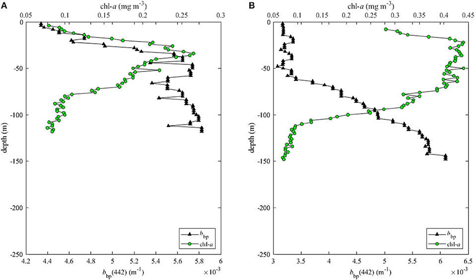
Figure 6. Vertical profiles of chlorophyll concentration (chl-a) and particulate backscattering at 442 nm [b_bp(442)] at (A) M66 station located close to McDonald Island and (B) T2 station located close to Heard at the beginning of Transect C.

FIGURE 7

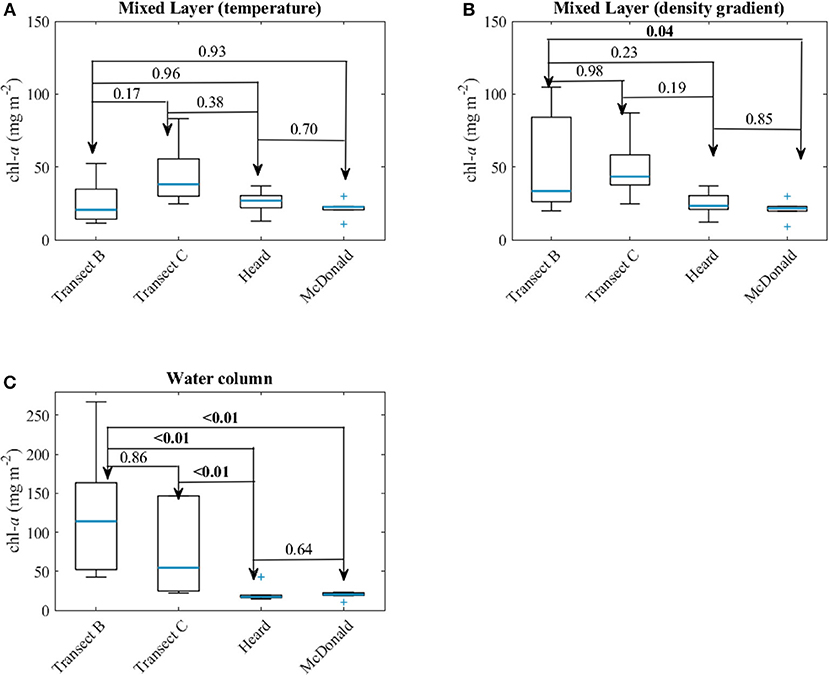
Figure 7. Chlorophyll a (chl-a) inventories (A) in the mixed layer calculated using the temperature criterion, (B) using the density gradient criterion, and (C) within the entire water column. The blue lines indicate the median and the box represents the range between 25 and 75% quartile and the whiskers correspond to ±2.7 standard deviation (99.3% of data if normally distributed). The numbers given are the p-values for the Kruskal-Wallis test. Numbers in bold indicate statistically significant differences.

Zooplankton Grazing

The accumulation of biomass is determined by the imbalance between the phytoplankton growth and loss due to grazing, mortality and export. The zooplankton grazing pressure varies for different phytoplankton groups. Generally, it is assumed that maximum grazing occurs for small phytoplankton (Wang and Moore, 2011) and the grazing pressure diminishes with increasing phytoplankton cell size (Acevedo-Trejos et al., 2015). Therefore, in areas dominated by smaller-sized species grazing should be the main control of the phytoplankton biomass. The phytoplankton community close to Heard and McDonald Islands was dominated by relatively small phytoplankton, i.e., nanoplankton (<20 μm; Figure 4), therefore the resulting increased growth rate of zooplankton may potentially lead to grazing control being dominant in this area, which hence could lead to decreased biomass concentration in the vicinity of the islands. Due to lack of any direct measurements of zooplankton abundance we looked at the content of degradation products of chl-a, i.e., chlorophyllide-a and phaeophorbide-a, as an indirect indicator of zooplankton grazing and phytoplankton mortality, via the presence of zooplankton fecal pellets and degradation of phytoplankton cells (Bidigare et al., 1986; DiTullio and Smith, 1996; Fundel et al., 1998). Increased chlorophyllide-a concentrations generally indicates cellular senescence of phytoplankton, whereas elevated phaeophorbide-a is generally a consequence of zooplankton activity, through transformation of chl-a and/or chlorophyllide-a (see Figure 1 in Bidigare et al., 1986). Ratios of both chlorophyllide a and phaeophorbide a to total chl-a concentration, were lower at the stations around Heard and McDonald Islands (Figure 8), however the difference was not statistically significant. Lower concentrations of chl-a degradation products, especially chlorophyllide a, indicates healthy, non-senescent, phytoplankton communities, as also indicated by the high F_v/F_m values above 0.5 in the vicinity of the islands (Figure 3C). The concentration of phaeophorbide a below the detection limit at stations close to HIMI suggest lower zooplankton activity in this area compared to the surrounding waters.

FIGURE 8

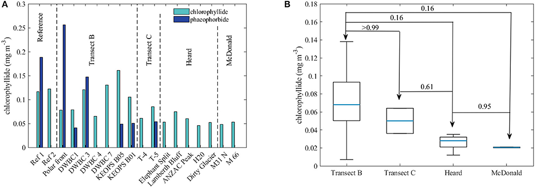
Figure 8. (A) Ratios of concentrations of degradation products of chlorophyll a (phaeophorbide and chlorophyllide) and total chlorophyll a concentration (chl-a) at all measurements stations, (B) average concentration of chlorophyllide in samples from reference, transect B and C, Heard and McDonald stations. All data presented in this figure are non-size-fractionated (total) concentrations. In the boxplot (B) the blue lines indicate the median and the box represents the range between 25 and 75% quartile and the whiskers correspond to ±2.7 standard deviation (99.3% of data if normally distributed). The numbers given are the p-values for the Kruskal-Wallis test.

Another indirect measure of possible increased grazing activity may be a change in the particulate organic carbon (POC) to particulate nitrogen (PN) ratios to chlorophyll a concentration. However, at all measurement stations the POC to PN ratios were close to the Redfield ratio of 6.625 (Redfield, 1934) and varied between 5.6 (station T-4) and 6.9 (M31N station) with the average values of 6.2, 6.2, 5.9 and 6.2 for reference, transect B, transect C, Heard and McDonald stations, respectively. It has also been recently observed that phytoplankton in the Southern Ocean can be grazed substantially by dinoflagellates (Christaki et al., 2015), but we found no evidence of the presence of dinoflagellates in our samples because at all stations close to HIMI the concentration of peridinin was below the detection limit. Measurable concentrations were only observed at Transect B stations and reference station #1. However, without the microscopic examination of the samples it is not possible to rule out the presence of dinoflagellates completely.

Light Limitation

Light availability has been considered as limiting factor for primary production in the Southern Ocean because of deep mixed layer depths, low sun angles and high cloud cover (e.g., Mitchell et al., 1991). Waters around Heard and McDonald Islands were characterized by relatively higher values of the particulate backscattering coefficient (Figure 9), which in this region was not correlated with chl-a concentration (Figure 10A). This indicates that water clarity in this area was strongly affected by non-algal particles (NAP), i.e., sediments and/or detritus. The source of this particulate material may be either the subglacial melting water as pointed out by van der Merwe et al. (2019) or the input of the resuspended sediments from the bottom due to the merging of the surface and bottom boundary layer due to deep mixing. High backscattering signal could be seen at depth at some stations relatively close to the islands, but with a mixed layer too shallow to mix up the sediments (Figure 6). Then at stations close to the islands and or at stations with mixed layers deep enough to reach the bottom boundary layer, the profiles of particulate backscattering were almost uniform (Figure 9).

FIGURE 9

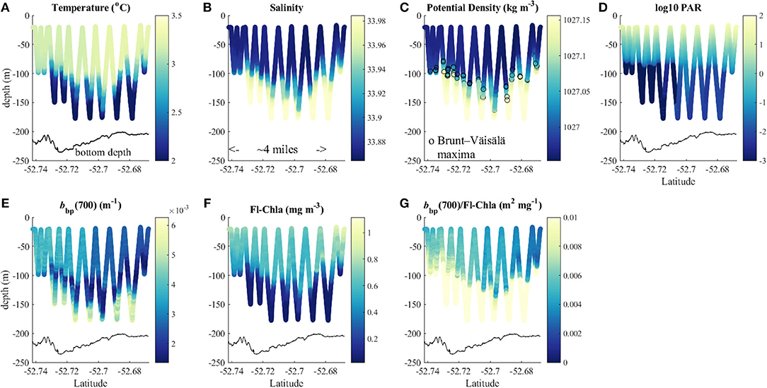
Figure 9. Triaxus transect (A) temperature (°C), (B) salinity, (C) potential density, (D) log₁₀(PAR), particulate backscattering coefficient at 700 nm [b_bp(700 nm)], (E) fluorescence derived chlorophyll a concentration (Fl-Chla), (F) ratio between particulate backscattering coefficient and chlorophyll a concentration [b_bp(700 nm)/Fl-Chla] (G); black line in each plot presents the bottom depth.

FIGURE 10

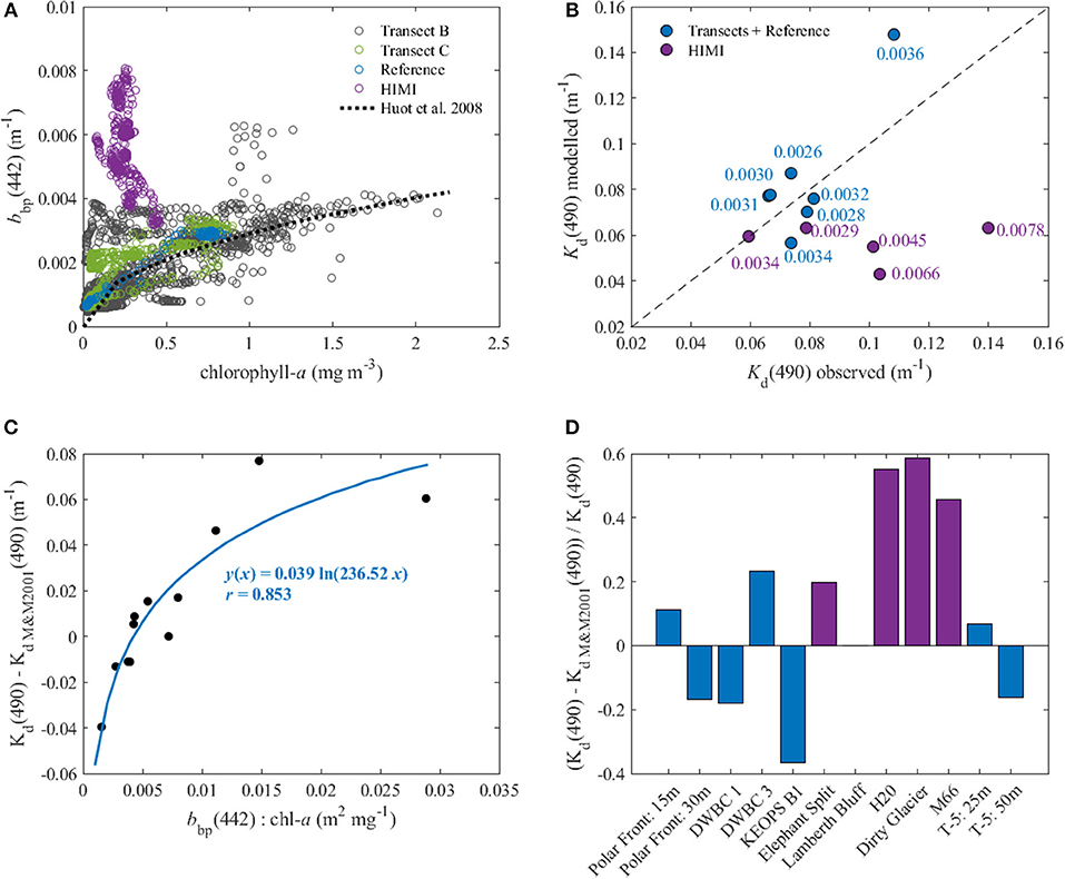
Figure 10. (A) Relationship between chlorophyll a concentration (chl-a) and particulate backscattering at 442 nm [b_bp(442)]; the black dotted line is the relationship between particulate backscattering coefficients at 442 nm and chl-a obtained for Case 1 waters (Huot et al., 2008); (B) comparison between the observed and modeled (Morel and Maritorena, 2001) values of K_d(490); the numbers are the values of b_bp(442) and the black dashed line is the 1:1 line; (C) dependency between K_{d_NAP}(490) { = K_d(490)—[K_{d_sw}(490) + K_{d_sw}(490)]} and the ratio between b_bp(442) and chl-a; the line is the best fit line to the data; (D) relative contribution of the light attenuation of non-algal particles to total light attenuation in the studied region.

The light attenuation in the water column can be described by the diffuse attenuation coefficient K_d, whose magnitude, in ocean waters, depends on the amount and optical properties of optically active seawater constituents like seawater itself (K_{d_sw}), phytoplankton and associated non-algal particles and CDOM (K_{d_bio}) and other non-algal substances (K_{d_NAP}):

$\begin{array}{ll}{K}_d(490)=K_{\text{d\_sw}}(490)+K_{\text{d\_bio}}(490)+K_{\text{d\_NAP}}(490)& (5)\end{array}$

In open ocean waters, where the contribution of non-algal particles not correlated to the chlorophyll concentration can be neglected (K_{d_NAP} = 0), the magnitude of the attenuation coefficient can be described by a relatively simple relationship with chl-a concentration, e.g., the one proposed by Morel and Maritorena (2001):

$\begin{array}{l}{K}_d\left(490\right)=K_{\text{d}\_\text{sw}}\left(490\right)+K_{\text{d}\_\text{bio}}\left(490\right)\\ =K_{\text{d}\_\text{MM2001}}\left(490\right)\\ =0.0166+0.07242{\left[\text{chl}-a\right]}^{0.68955}& (6)\end{array}$

For transect B and C and reference stations, we found good agreement between modeled and measured K_d(490), whereas at the stations close to Heard and McDonald Islands, that were characterized by relatively high values of the particulate backscattering coefficient, the model underestimated the value of K_d(490) by ~2-fold (Figure 10B). This indicates that in this region the attenuation of light by non-algal particles (K_{d_NAP}), most probably sediments present in the water column due to the merge of the surface and benthic boundary layers, plays a significant role in light limitation.

Changes in the particulate matter composition can be detected when looking at the ratio between backscattering coefficient and chl-a concentration (e.g., Barbieux et al., 2018). In the data from the Triaxus transect, a clear shift in this ratio could be observed with relatively high values in the areas close to Heard Island and gradually decreasing with increasing distance from the island (Figure 9). In our data set we found a strong (r = 0.85) relation between K_{d_NAP}(490) and the backscattering at 442 nm and chl-a ratio (Figure 10C). Using this approximation of K_{d_NAP}(490) in Equation (5) and assuming the relationship between K_{d_bio}(490) to stay the same as in the Morel and Maritorena (2001) model substantially improved the fit between modeled and observed values of K_d(490) in all regions, including the shallow coastal areas.

The values of K_d(PAR) did not show a clear spatial pattern in the study area. No increase was observed at the coastal stations, despite their higher b_bp values. However, deep vertical mixing, apart from dilution of biomass within the water column mentioned before, influences phytoplankton production and phenology also by controlling the balance between nutrient (including Fe) supply from greater depths and the light limitation through decreasing the mean light levels within the mixed layer (Ardyna et al., 2017; Llort et al., 2019). To compare the availability of light that may be used by the phytoplankton for primary production we calculated the median irradiance within the mixed layer (ML), PAR_ML (Behrenfeld et al., 2015):

$\begin{array}{ll}PA{R}_{ML}=PAR(z=0)\times e^{-0.5K_d(PAR)\times MLD}& (7)\end{array}$

and the average irradiance within the mixed layer as done by Blain et al. (2013):

$\begin{array}{ll}\overline{PA{R}_{ML}}=\frac{PAR(z=0)}{K_d(PAR)xMLD}(1-e^{-K_d(PAR)\times MLD})& (8)\end{array}$

We investigated both of these parameters, given it is has not been resolved as to whether phytoplankton acclimate to daily mean or median light levels within the mixed layer (Graff and Behrenfeld, 2018). The average daily surface PAR was retrieved from the MODIS-Aqua monthly remote sensing products captured between 2002 and 2017 (and released by NASA) by extracting the monthly data for the region situated in the Kerguelen Plateau (see region B in Figure 1). The yearly variability of surface PAR is shown in Figure 11A. For example, the average daily doses of PAR in the vicinity of Heard and McDonald Islands (Region C in Figure 1) were 28.67 ± 4.25 and 19.46 ± 2.28 mol photons m⁻² day⁻¹ in January and February, respectively. The highest daily dose of PAR at the surface of 39.80 ± 4.26 mol photons m⁻² day⁻¹ in this region was observed in November (Figure 11A).

FIGURE 11

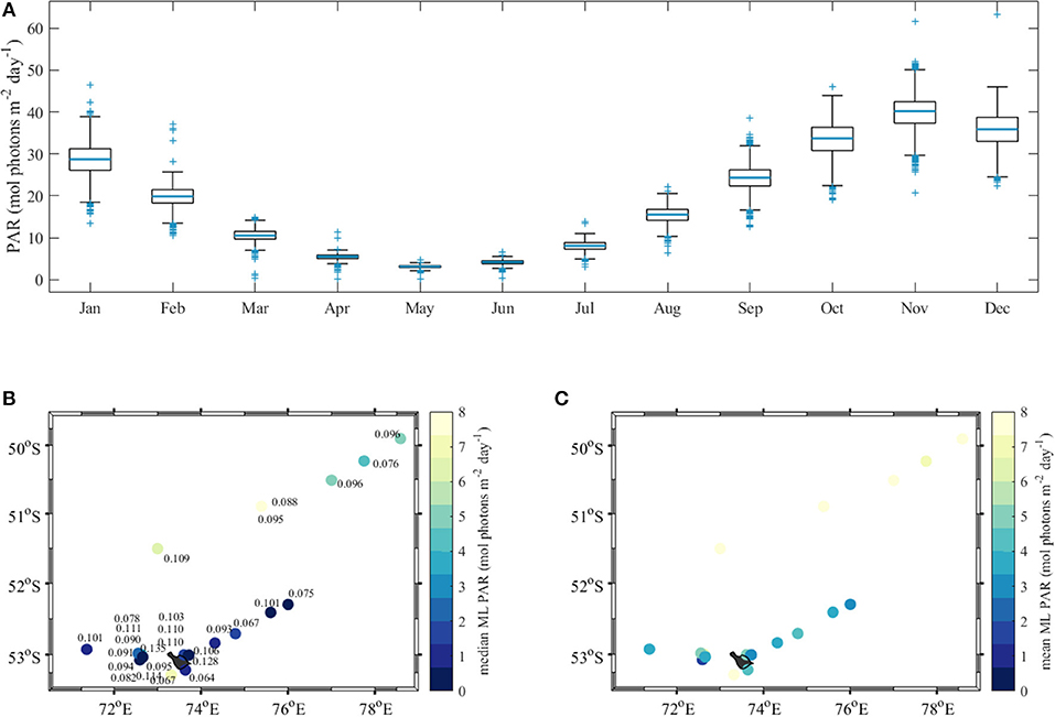
Figure 11. (A) Monthly surface daily PAR dose in the vicinity of Heard and McDonald islands between 2002 and 2017; (B) median and (C) average mixed layer daily doses of PAR. In the boxplot (A) the blue lines indicate the median and the box represents the range between 25 and 75% quartile and the whiskers correspond to ±2.7 standard deviation (99.3% of data if normally distributed). The numbers in (B) are the K_d(PAR) values.

Next, the magnitude of PAR just below the surface was calculated allowing for a 7.6% reduction of the above surface PAR (Morel, 1991). For the assessment of the light availability within the ML we chose the average value observed in this region in summer (December–February) assuming constant surface insolation at all stations and using K_d(PAR) and MLD values calculated from our in situ profiles. Among all stations, K_d(PAR) varied by about a factor 2, with minimum K_d(PAR) values of 0.064 m⁻¹ south of Heard Island to 0.128 m⁻¹ north of Heard Island, measured at the station directly affected by the glacier outflow (van der Merwe et al., 2019) (Figure 11B).

The median of the average daily dose of PAR within the mixed layer showed a clear distinction between Transect B and the rest of the stations, which were closer to the islands. Transect B stations received much higher daily doses of PAR than stations near the islands, including Transect C, with one exception south of Heard Island. In the areas close to Heard Island and on Transect C, the median daily dose of PAR within the mixed layer was 4.2, 3.3, and 2.3 mol photons m⁻² day⁻¹ for the average December, January, and February surface PAR levels (Figure 12). A previous Southern Ocean study found that average light levels below 3.5 mol photons m⁻² day⁻¹ indicated light limiting conditions (Blain et al., 2013), suggesting that in January and February most Heard Island and Transect C stations were light limited. Interestingly, we did not observe much variability in both mean and median mixed layer PAR between HIMI and Transect C stations (Figures 11B,C) even though the non-algal particle loading was much more significant at the HIMI stations (Figure 10D). While on Transect C self-shading by the phytoplankton paired with deep mixed layers was the main driver for the light reduction, light attenuation by mineral suspensions was significant in the shallower regions around the islands, being responsible for more than 50% of the decrease in light intensity (Figure 10D). As a result, the point at which the light availability starts to be limiting for phytoplankton was reached at lower biomass levels, thus capping the amount of phytoplankton that could be maintained. This contention is also supported by the fact that the PAR profiles measured in the study region did not reveal any decrease in the euphotic depth close to the island (Table 2). The median and average light levels are of course dependent on the choice of MLD criterion, and using the deeper MLD obtained with the alternate maximum density gradient criterion (see Methods section Sampling and Oceanographic Measurements), the differences between the HIMI and transect B sites are reduced, with essentially all sites exhibiting close to limiting light levels. This does not change the conclusion that biomass concentrations proceed until light limitation arises, with lower biomass accumulation occurring near the islands where non-algal particles reduce light penetration.

FIGURE 12

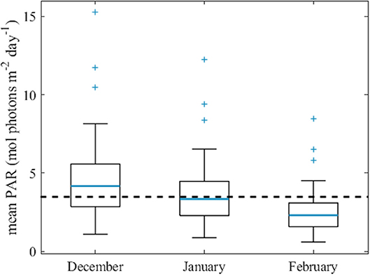
Figure 12. Average daily dose of PAR within the mixed layer for the Heard and McDonald Islands and transect C stations. The average monthly surface PAR obtained from MODIS-Aqua was used for the calculations. Black dashed line represents mean daily PAR of 3.5 mol photons m⁻² day⁻¹ and indicates light limitation conditions (Blain et al., 2013).

Therefore, it is probable that the phytoplankton growth at both HIMI and transect C stations was light limited (and also within the deeper portions of the water column at the transect B stations). One could also expect that the composition of photoprotective (PP) and photosynthetic (PS) pigments would reflect differences in the light regimes in different regions because the underwater light field properties, both light intensity and chromatic composition, directly affect pigment composition in phytoplankton (e.g., Falkowski and LaRoche, 1991). However, we have found no statistically significant differences between relative concentrations of either PP or PS carotenoids within the mixed layer in the different regions (Kruskal-Wallis test, p < 0.05); possibly reflecting the generally low light levels at all sites. Significantly lower concentrations of accessory chlorophylls (Kruskal-Wallis test, p < 0.05) were observed in the samples collected close to HIMI, and are possibly primarily the result of the different, smaller cell, community that was present.

Dilution of Biomass Through Lateral Mixing

In addition to light limitation, it is possible that the lower chl-a accumulation near HIMI occurs in part because this region is close to the edge of the plateau, so that dilution via mixing with surrounding low chl-a waters reduces biomass in comparison to the central plateau. The spatial distribution of this lateral dilution has been mapped, in units of water mass residence times in days, using a high resolution tide and wind driven mixing model (Maraldi et al., 2009). The model suggests that residence times are >10 days over the central plateau and decrease to 2–5 days in the region north of HIMI (their Figure 7) where both satellite and our in-situ observations show lower biomass. As a first assessment of whether this shorter residence time can explain the lower biomass, requires we use scaling arguments. Accumulation of phytoplankton biomass expressed in chl-a concentration from its initial off plateau level chl-a₀ over the residence time τ at a net daily rate μ can be described by:

$\begin{array}{ll}\text{chl}-a={\text{chl}-a}_0{e}^{(\mu \tau )}& (9)\end{array}$

The net accumulation rate in the iron-fertilized waters over the central plateau must be high enough to yield the observed chl-a concentrations (0.5 to 2.5 mg m⁻³) within the residence time. This suggests μ must be >0.2 d⁻¹. For example, starting from a winter chl₀ value of 0.03, 20 days are required to reach 1.6 mg m⁻³, or 15 days starting from a spring chl-a₀ value of 0.1 mg m⁻³ (both for μ = 0.2 d⁻¹). These times are similar or longer than the time of ~2 weeks to reach this biomass level in spring as seen in satellite ocean color images (Blain et al., 2007; Maraldi et al., 2009). Conversely, μ is unlikely to be >0.3 d⁻¹, or biomass would exceed 2 mg m⁻³ within 10 days and 9 mg m⁻³ by 15 days—rates and peak accumulations that are higher than those observed.

With these bounds of 0.2 < μ < 0.3 d⁻¹ we can assess whether the variation in residence time is sufficient to explain the difference in biomass levels, by writing (Equation 9) for our two locations with different residence times (τ_central and τ_edge) and solving for the biomass ratio:

$\begin{array}{ll}\frac{{\text{chl}-a}_{\text{central}}}{{\text{chl}-a}_{edge}}=R_{\text{chl}-a}=e^{-\mu ({\tau }_{\text{central}}-{\tau }_{\text{edge}})}={\text{e}}^{-\mu (\delta \tau )}& (10)\end{array}$

For (δτ) of 10 days, R_chl is in the range 0.05 to 0.14 (for 0.2 < μ < 0.3 d⁻¹), and thus when the central bloom has reached 3 mg m⁻³, lateral dilution would reduce the levels near HIMI to 0.15 to 0.42 mg m⁻³ (above the background HNLC off-plateau levels of ~0.25 mg m⁻³), which is similar to the levels observed.

This scaling emphasizes that lateral mixing is likely to be a significant factor in the observation of the low biomass “halo” around the islands. Nonetheless, other factors are also likely to be important, as we have emphasized above, and are required to explain the observed community structure variations.

Possible Explanations for the Changes in the Phytoplankton Community Structure

The phytoplankton community close to both Heard and McDonald Islands was generally dominated by nanoplankton. The relatively high concentration of 19′-HF indicates an increase of the contribution of haptophytes, most probably Phaeocystis spp. due to relatively high concentrations of 19′-BF (Zapata et al., 2004), compared to diatoms close to Heard and McDonald Islands, especially in the <20 μm fraction (Figure 4C). Similarly, Iida and Odate (2014) observed domination of phytoplankton smaller than 10 μm and based on CHEMTAX analysis they found domination of haptophyte type 4 (i.e., Phaeocystis antarctica) at latitudes between 50 and 54°S.

Even though, diatoms are the main phytoplankton group dominating in the Southern Ocean, Phaeocystis blooms have been observed in some regions (DiTullio et al., 2000; Smith and Asper, 2001; Poulton et al., 2007; Feng et al., 2010). The changes in the dominant species have been explained by the different response of diatoms and haptophytes to the light conditions induced by mixing. In the Ross Sea, for example, diatom-dominated communities were mostly found in highly-stratified waters, whereas Phaeocystis antarctica communities typically prevailed in deeply mixed waters (Arrigo, 1999). Therefore, the most possible environmental factor controlling the composition of the community in the waters surrounding HIMI was deep mixing and the associated light regime in this region (Figure 10). In this study we found a strong positive correlation between the mixed layer depth and the ratios between chlorophyll a and 19′-HF (r > 0.83) and 19′-BF (r > 0.77) concentration in both the total (Figure 13A) and <20 μm (Figure 13B) phytoplankton size fractions. The prevalence of Phaeocystis spp. in deeply mixed regimes most probably results from relatively faster photorecovery of Phaeocystis spp. compared to diatom species, suggesting better adaptation to fluctuating light regimes (Tozzi et al., 2017). Other observations have indicated that Phaeocystis spp. adapts better to low light conditions and can be found even below the sea ice (e.g., Tang et al., 2009) and therefore can compete with diatoms. By comparison, Feng et al. (2010) in their incubation experiments under high light conditions, observed increased abundances of Phaeocystis spp. compared to diatoms.

FIGURE 13

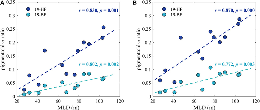
Figure 13. Relation between mixed layer depth (MLD) and ratios between 19′-hexanoyloxyfucoxanthin (19-HF), 19′-butanoyloxyfucoxanthin (19-BF), and chlorophyll a concentration (chl-a) in (A) the total and (B) <20 μm size fraction.

Looking at the relation between MLD and Phaeocystis abundance through the ratios of 19′-HF and 19′-BF to chl-a is very simplistic, as these ratios are strongly dependent on iron availability and they increase when moving from high to low iron concentrations (DiTullio et al., 2007; van Leeuwe et al., 2014). Additionally, the increase in the abundance of haptophytes may be caused by the higher dissolved iron concentration in the vicinity of the islands itself. Iron addition experiments in the Ross Sea clearly showed strong response of Phaeocystis spp. to iron addition, which resulted in a switch of the phytoplankton community structure from diatoms to Phaeocystis spp. (Coale et al., 2003), indicating that iron distribution plays an important role in controlling the distribution of various phytoplankton groups in the Southern Ocean. Also in the SOIREE experiment (Boyd et al., 2000) the phytoplankton response in the few initial days after Fe addition was a relative increase in the autotrophic flagellates (mainly haptophytes), and only after 6 days the shift into a diatom-dominated community was observed.

Conclusions

The HIMI region is a very dynamic system, experiencing intense inputs of the micro-nutrient iron from glaciers and volcanic islands into coastal waters that are rapidly mixed by the high winds and strong currents that are typical for the Southern Ocean. The iron inputs stimulate phytoplankton growth, but the dynamics limit biomass accumulation via multiple processes. Near the edge of the plateau, the biomass is diluted by horizontal mixing with surrounding waters in the Antarctic Circumpolar Current. Deep wind-induced mixing reduces light levels, slowing growth. Near the islands, this wind mixing reaches into the benthic boundary layers and re-suspends sediments that further limits light availability, producing a halo of low biomass despite the iron enrichment. This case study demonstrates the importance of considering overall system dynamics, including nutrient/light availability and local circulation, in the assessment of Southern Ocean ecosystem.

Data Availability

The datasets generated for this study are available on request to the corresponding author.

Author Contributions

BW and TT conceived the study and carried out the field work. LC, DD, and NP analyzed samples. All authors contributed to manuscript revision, read, and approved the submitted version.

Funding

BW was funded via a CSIRO Office of the Chief Executive Postdoctoral Fellowship. Fieldwork was supported by the Australian Marine National Facility and the ACE CRC.

Conflict of Interest Statement

NP was employed by company JBS&G.

The remaining authors declare that the research was conducted in the absence of any commercial or financial relationships that could be construed as a potential conflict of interest.

Acknowledgments

We thank the officers, crew, and science party of RV Investigator Voyage IN2016-01 for support and good cheer. The ocean color data were obtained from ESA OC-CCI http://www.esa-oceancolour-cci.org/ and NASA https://oceandata.sci.gsfc.nasa.gov/MODIS-Aqua/.

References

AAD and Director of National Parks (2005). Heard Island and McDonald Islands Marine Reserve Management Plan. Kingston, ACT: Australian Antarctic Division.

Acevedo-Trejos, E., Brandt, G., Bruggeman, J., and Merico, A. (2015). Mechanisms shaping size structure and functional diversity of phytoplankton communities in the ocean. Sci. Rep. 5:8918. doi: 10.1038/srep08918

PubMed Abstract | CrossRef Full Text | Google Scholar

Alderkamp, A., van Dijken, G., Lowry, K., Lewis, K., Joy-Warren H, L., de Poll, W., et al. (2019). Effects of iron and light availability on phytoplankton photosynthetic properties in the Ross Sea. Mar. Ecol. Prog. Ser. 621, 33–50. doi: 10.3354/meps13000

CrossRef Full Text | Google Scholar

Ardyna, M., Claustre, H., Sallée, J.-B., D'Ovidio, F., Gentili, B., van Dijken, G., et al. (2017). Delineating environmental control of phytoplankton biomass and phenology in the Southern Ocean: phytoplankton dynamics in the SO. Geophys. Res. Lett. 44, 5016–5024. doi: 10.1002/2016GL072428

CrossRef Full Text | Google Scholar

Armand, L. K., Cornet-Barthaux, V., Mosseri, J., and Quéguiner, B. (2008). Late summer diatom biomass and community structure on and around the naturally iron-fertilised Kerguelen Plateau in the Southern Ocean. Deep Sea Res. Part II Top. Stud. Oceanogr. 55, 653–676. doi: 10.1016/j.dsr2.2007.12.031

CrossRef Full Text | Google Scholar

Arrigo, K. R. (1999). Phytoplankton community structure and the drawdown of nutrients and CO₂ in the Southern Ocean. Science 283, 365–367. doi: 10.1126/science.283.5400.365

PubMed Abstract | CrossRef Full Text | Google Scholar

Barbieux, M., Uitz, J., Bricaud, A., Organelli, E., Poteau, A., Schmechtig, C., et al. (2018). Assessing the variability in the relationship between the particulate backscattering coefficient and the chlorophyll a concentration from a global biogeochemical-argo database. J. Geophys. Res. Oceans 123, 1229–1250. doi: 10.1002/2017JC013030

CrossRef Full Text | Google Scholar

Behrenfeld, M. J., O'Malley, R. T., Boss, E. S., Westberry, T. K., Graff, J. R., Halsey, K. H., et al. (2015). Revaluating ocean warming impacts on global phytoplankton. Nat. Clim. Change 6, 323–330. doi: 10.1038/nclimate2838

CrossRef Full Text | Google Scholar

Bidigare, R. R., Frank, T. J., Zastrow, C., and Brooks, J. M. (1986). The distribution of algal chlorophylls and their degradation products in the Southern Ocean. Deep Sea Res. Part Oceanogr. Res. Pap. 33, 923–937. doi: 10.1016/0198-0149(86)90007-5

CrossRef Full Text | Google Scholar

Blain, S., Quéguiner, B., Armand, L., Belviso, S., Bombled, B., Bopp, L., et al. (2007). Effect of natural iron fertilization on carbon sequestration in the Southern Ocean. Nature 446, 1070–1074. doi: 10.1038/nature05700

PubMed Abstract | CrossRef Full Text | Google Scholar

Blain, S., Quéguiner, B., and Trull, T. (2008). The natural iron fertilization experiment KEOPS (KErguelen Ocean and Plateau compared Study): an overview. Deep Sea Res. Part II Top. Stud. Oceanogr. 55, 559–565. doi: 10.1016/j.dsr2.2008.01.002

CrossRef Full Text | Google Scholar

Blain, S., Renaut, S., Xing, X., Claustre, H., and Guinet, C. (2013). Instrumented elephant seals reveal the seasonality in chlorophyll and light-mixing regime in the iron-fertilized Southern Ocean: chlorophyll and light in Southern Ocean. Geophys. Res. Lett. 40, 6368–6372. doi: 10.1002/2013GL058065

CrossRef Full Text | Google Scholar

Blain, S., Tréguer, P., Belviso, S., Bucciarelli, E., Denis, M., Desabre, S., et al. (2001). A biogeochemical study of the island mass effect in the context of the iron hypothesis: Kerguelen Islands, Southern Ocean. Deep Sea Res. Part Oceanogr. Res. Pap. 48, 163–187. doi: 10.1016/S0967-0637(00)00047-9

CrossRef Full Text | Google Scholar

Boyd, P. W., Arrigo, K. R., Strzepek, R., and van Dijken, G. L. (2012). Mapping phytoplankton iron utilization: insights into Southern Ocean supply mechanisms. J. Geophys. Res. Oceans 117:C06009. doi: 10.1029/2011JC007726

CrossRef Full Text | Google Scholar

Boyd, P. W., Watson, A. J., Law, C. S., Abraham, E. R., Trull, T., Murdoch, R., et al. (2000). A mesoscale phytoplankton bloom in the polar Southern Ocean stimulated by iron fertilization. Nature 407, 695–702. doi: 10.1038/35037500

PubMed Abstract | CrossRef Full Text | Google Scholar

Brainerd, K. E., and Gregg, M. C. (1995). Surface mixed and mixing layer depths. Deep Sea Res. Part Oceanogr. Res. Pap. 42, 1521–1543. doi: 10.1016/0967-0637(95)00068-H

CrossRef Full Text | Google Scholar

Briggs, N., Perry, M. J., Cetinić, I., Lee, C., D'Asaro, E., Gray, A. M., et al. (2011). High resolution observations of aggregate flux during a sub-polar North Atlantic spring bloom. Deep Sea Res. I 58, 1031–1039. doi: 10.1016/j.dsr.2011.07.007

CrossRef Full Text | Google Scholar

Carvalho, F., Kohut, J., Oliver, M. J., and Schofield, O. (2017). Defining the ecologically relevant mixed-layer depth for Antarctica's coastal seas: MLD in Coastal Antarctica. Geophys. Res. Lett. 44, 338–345. doi: 10.1002/2016GL071205

CrossRef Full Text | Google Scholar

Christaki, U., Georges, C., Genitsaris, S., and Monchy, S. (2015). Microzooplankton community associated with phytoplankton blooms in the naturally iron-fertilized Kerguelen area (Southern Ocean). FEMS Microbiol. Ecol. 91:fiv068. doi: 10.1093/femsec/fiv068

PubMed Abstract | CrossRef Full Text | Google Scholar

Clementson, L. A. (2012). “The CSIRO method,” in The Fifth SeaWiFS HPLS Analysis Round-Robin Experiment (SeaHARRE-5) NASA Technical Memorandum 2012-217503, eds S. B. Hooker, L. Clementson, C. S. Thomas, L. Schlüter, M. Allerup, J. Ras, et al. (Greenbelt, MD: NASA Goddard Space Flight Center), 44–50.

Google Scholar

Coale, K. H., Johnson, K. S., Chavez, F. P., Buesseler, K. O., Barber, R. T., Brzezinski, M. A., et al. (2004). Southern Ocean iron enrichment experiment: carbon cycling in high- and low-Si waters. Science 304, 408–414. doi: 10.1126/science.1089778

PubMed Abstract | CrossRef Full Text | Google Scholar

Coale, K. H., Wang, X., Tanner, S. J., and Johnson, K. S. (2003). Phytoplankton growth and biological response to iron and zinc addition in the Ross Sea and Antarctic Circumpolar Current along 170°W. Deep Sea Res. Part II Top. Stud. Oceanogr. 50, 635–653. doi: 10.1016/S0967-0645(02)00588-X

CrossRef Full Text | Google Scholar

de Boyer Montégut, C., Madec, G., Fischer, A. S., Lazar, A., and Iudicone, D. (2004). Mixed layer depth over the global ocean: an examination of profile data and a profile-based climatology. J. Geophys. Res. 109:C12003. doi: 10.1029/2004JC002378

CrossRef Full Text | Google Scholar

de Jong, J., Schoemann, V., Lannuzel, D., Croot, P., de Baar, H., and Tison, J.-L. (2012). Natural iron fertilization of the Atlantic sector of the Southern Ocean by continental shelf sources of the Antarctic Peninsula. J. Geophys. Res. Biogeosci. 117:G01029. doi: 10.1029/2011JG001679

CrossRef Full Text | Google Scholar

DiTullio, G. R., Garcia, N., Riseman, S. F., and Sedwick, P. N. (2007). “Effects of iron concentration on pigment composition in Phaeocystis antarctica grown at low irradiance,” in Phaeocystis, Major Link in the Biogeochemical Cycling of Climate-Relevant Elements, eds M. A. van Leeuwe, J. Stefels, S. Belviso, C. Lancelot, P. G. Verity, and W. W. C. Gieskes (Dordrecht: Springer, 71–81.

Google Scholar

DiTullio, G. R., Grebmeier, J. M., Arrigo, K. R., Lizotte, M. P., Robinson, D. H., Leventer, A., et al. (2000). Rapid and early export of Phaeocystis antarctica blooms in the Ross Sea, Antarctica. Nature 404, 595–598. doi: 10.1038/35007061

PubMed Abstract | CrossRef Full Text | Google Scholar

DiTullio, G. R., and Smith, W. O. (1996). Spatial patterns in phytoplankton biomass and pigment distributions in the Ross Sea. J. Geophys. Res. Oceans 101, 18467–18477. doi: 10.1029/96JC00034

CrossRef Full Text | Google Scholar

Falkowski, P. G., and LaRoche, J. (1991). Acclimation to spectral irradiance in algae. J. Phycol. 27, 8–14. doi: 10.1111/j.0022-3646.1991.00008.x

CrossRef Full Text | Google Scholar

Feng, Y., Hare, C. E., Rose, J. M., Handy, S. M., DiTullio, G. R., Lee, P. A., et al. (2010). Interactive effects of iron, irradiance and CO₂ on Ross Sea phytoplankton. Deep Sea Res. Part Oceanogr. Res. Pap. 57, 368–383. doi: 10.1016/j.dsr.2009.10.013

CrossRef Full Text | Google Scholar

Field, C. B., Behrenfeld, M. J., Randerson, J. T., and Falkowski, P. (1998). Primary production of the biosphere: integrating terrestrial and oceanic components. Science 281, 237–240. doi: 10.1126/science.281.5374.237

PubMed Abstract | CrossRef Full Text | Google Scholar

Fundel, B., Stich, H.-B., Schmid, H., and Maier, G. (1998). Can phaeopigments be used as markers for Daphnia grazing in Lake Constance? J. Plankton Res. 20, 1449–1462. doi: 10.1093/plankt/20.8.1449

CrossRef Full Text | Google Scholar

Gall, M. P., Strzepek, R., Maldonado, M., and Boyd, P. W. (2001). Phytoplankton processes. Part 2: rates of primary production and factors controlling algal growth during the Southern Ocean Iron RElease Experiment (SOIREE). Deep Sea Res. Part II Top. Stud. Oceanogr. 48, 2571–2590. doi: 10.1016/S0967-0645(01)00009-1

CrossRef Full Text | Google Scholar

Gordon, H. R., and McCluney, W. R. (1975). Estimation of the depth of sunlight penetration in the sea for remote sensing. Appl.Opt. 14, 413–416. doi: 10.1364/AO.14.000413

PubMed Abstract | CrossRef Full Text | Google Scholar

Graff, J. R., and Behrenfeld, M. J. (2018). Photoacclimation responses in Subarctic Atlantic phytoplankton following a natural mixing-restratification event. Front. Mar. Sci. 5:209. doi: 10.3389/fmars.2018.00209

CrossRef Full Text | Google Scholar

Grenier, M., Della Penna, A., and Trull, T. W. (2015). Autonomous profiling float observations of the high-biomass plume downstream of the Kerguelen Plateau in the Southern Ocean. Biogeosciences 12, 2707–2735. doi: 10.5194/bg-12-2707-2015

CrossRef Full Text | Google Scholar

Harvey, M. J., Law, C. S., Smith, M. J., Hall, J. A., Abraham, E. R., Stevens, C. L., et al. (2011). The SOLAS air–sea gas exchange experiment (SAGE) 2004. Deep Sea Res. Part II Top. Stud. Oceanogr. 58, 753–763. doi: 10.1016/j.dsr2.2010.10.015

CrossRef Full Text | Google Scholar

Hatta, M., Measures, C. I., Selph, K. E., Zhou, M., and Hiscock, W. T. (2013). Iron fluxes from the shelf regions near the South Shetland Islands in the Drake Passage during the austral-winter 2006. Deep Sea Res. Part II Top. Stud. Oceanogr. 90, 89–101. doi: 10.1016/j.dsr2.2012.11.003

CrossRef Full Text | Google Scholar

Holmes, T. M., Chase, Z., van der Merwe, P., Townsend, A. T., and Bowie, A. R. (2017). Detection, dispersal and biogeochemical contribution of hydrothermal iron in the ocean. Mar. Freshw. Res. 68, 2184–2204. doi: 10.1071/MF16335

CrossRef Full Text | Google Scholar

Holmes, T. M., Wuttig, K., Chase, Z., van der Merwe, P., Townsend, A. T., Schallenberg, C., et al. (2019). Iron availability influences nutrient drawdown in the Heard and McDonald Island region, Southern Ocean. Mar. Chem. 211, 1–14. doi: 10.1016/j.marchem.2019.03.002

CrossRef Full Text | Google Scholar

Huot, Y., Morel, A., Twardowski, M. S., Stramski, D., and Reynolds, R. A. (2008). Particle optical backscattering along a chlorophyll gradient in the upper layer of the eastern South Pacific Ocean. Biogeosciences 5, 495–507. doi: 10.5194/bg-5-495-2008

CrossRef Full Text | Google Scholar

Iida, T., and Odate, T. (2014). Seasonal variability of phytoplankton biomass and composition in the major water masses of the Indian Ocean sector of the Southern Ocean. Polar Sci. 8, 283–297. doi: 10.1016/j.polar.2014.03.003

CrossRef Full Text | Google Scholar

Jickells, T. D., An, Z. S., Andersen, K. K., Baker, A. R., Bergametti, G., Brooks, N., et al. (2005). Global iron connections between desert dust, ocean biogeochemistry, and climate. Science 308, 67–71. doi: 10.1126/science.1105959

PubMed Abstract | CrossRef Full Text | Google Scholar

Kolber, Z. S., Prášil, O., and Falkowski, P. G. (1998). Measurements of variable chlorophyll fluorescence using fast repetition rate techniques: defining methodology and experimental protocols. Biochim. Biophys. Acta 1367, 88–106. doi: 10.1016/S0005-2728(98)00135-2

PubMed Abstract | CrossRef Full Text | Google Scholar

Lacour, L., Ardyna, M., Stec, K. F., Claustre, H., Prieur, L., Poteau, A., et al. (2017). Unexpected winter phytoplankton blooms in the North Atlantic subpolar gyre. Nat. Geosci. 10, 836–839. doi: 10.1038/ngeo3035

CrossRef Full Text | Google Scholar

Lacour, L., Briggs, N., Claustre, H., Ardyna, M., and Dall'Olmo, G. (2019). The intra-seasonal dynamics of the mixed layer pump in the subpolar North Atlantic Ocean: a BGC-Argo float approach. Glob. Biogeochem. Cycles 33, 266–281. doi: 10.1029/2018GB005997

CrossRef Full Text | Google Scholar

Llort, J., Lévy, M., Sallée, J. B., and Tagliabue, A. (2019). Nonmonotonic response of primary production and export to changes in mixed-layer depth in the Southern Ocean. Geophys. Res. Lett. 46, 3368–3377. doi: 10.1029/2018GL081788

CrossRef Full Text | Google Scholar

Lupton, J. E., Arculus, R. J., Coffin, M. J., Bradney, A., Baumberger, T., and Wilkinson, C. (2017). Hydrothermal Venting on the Flanks of Heard and Mcdonald Islands, Southern Indian Ocean. New Orleans, LA: American Geophysical Union.

Google Scholar

Maffione, R. A., and Dana, D. R. (1997). Instruments and methods for measuring the backward-scattering coefficient of ocean waters. Appl. Opt. 36, 6057–6067. doi: 10.1364/AO.36.006057

PubMed Abstract | CrossRef Full Text | Google Scholar

Mahowald, N. M., Baker, A. R., Bergametti, G., Brooks, N., Duce, R. A., Jickells, T. D., et al. (2005). Atmospheric global dust cycle and iron inputs to the ocean. Glob. Biogeochem. Cycles 19:GB4025. doi: 10.1029/2004GB002402

CrossRef Full Text | Google Scholar

Maraldi, C., Mongin, M., Coleman, R., and Testut, L. (2009). The influence of lateral mixing on a phytoplankton bloom: distribution in the Kerguelen Plateau region. Deep Sea Res. Part Oceanogr. Res. Pap. 56, 963–973. doi: 10.1016/j.dsr.2008.12.018

CrossRef Full Text | Google Scholar

Martin, J. H., Gordon, R. M., and Fitzwater, S. E. (1990). Iron in Antarctic waters. Nature 345, 156–158. doi: 10.1038/345156a0

CrossRef Full Text | Google Scholar

Martin, P., van der Loeff, M. R., Cassar, N., Vandromme, P., d'Ovidio, F., Stemmann, L., et al. (2013). Iron fertilization enhanced net community production but not downward particle flux during the Southern Ocean iron fertilization experiment LOHAFEX: NCP AND PARTICLE FLUX DURING LOHAFEX. Glob. Biogeochem. Cycles 27, 871–881. doi: 10.1002/gbc.20077

CrossRef Full Text | Google Scholar

Mitchell, B. G., Brody, E. A., Holm-Hansen, O., McClain, C., and Bishop, J. (1991). Light limitation of phytoplankton biomass and macronutrient utilization in the Southern Ocean. Limnol. Oceanogr. 36, 1662–1677. doi: 10.4319/lo.1991.36.8.1662

CrossRef Full Text | Google Scholar

Mongin, M., Molina, E., and Trull, T. W. (2008). Seasonality and scale of the Kerguelen plateau phytoplankton bloom: a remote sensing and modeling analysis of the influence of natural iron fertilization in the Southern Ocean. Deep Sea Res. Part II Top. Stud. Oceanogr. 55, 880–892. doi: 10.1016/j.dsr2.2007.12.039

CrossRef Full Text | Google Scholar

Moore, J. K., and Braucher, O. (2008). Sedimentary and mineral dust sources of dissolved iron to the world ocean. Biogeosciences 5, 631–656. doi: 10.5194/bg-5-631-2008

CrossRef Full Text | Google Scholar

Morel, A. (1991). Light and marine photosynthesis: a spectral model with geochemical and climatological implications. Prog. Oceanogr. 26, 263–306. doi: 10.1016/0079-6611(91)90004-6

CrossRef Full Text | Google Scholar

Morel, A., and Maritorena, S. (2001). Bio-optical properties of oceanic waters: a reappraisal. J. Geophys. Res. 106, 7163–7180. doi: 10.1029/2000JC000319

CrossRef Full Text | Google Scholar

Park, Y.-H., Fuda, J.-L., Durand, I., and Naveira Garabato, A. C. (2008). Internal tides and vertical mixing over the Kerguelen Plateau. Deep Sea Res. Part II Top. Stud. Oceanogr. 55, 582–593. doi: 10.1016/j.dsr2.2007.12.027

CrossRef Full Text | Google Scholar

Peloquin, J., Hall, J., Safi, K., Smith, W. O., Wright, S., and van den Enden, R. (2011). The response of phytoplankton to iron enrichment in Sub-Antarctic HNLCLSi waters: results from the SAGE experiment. Deep Sea Res. Part II Top. Stud. Oceanogr. 58, 808–823. doi: 10.1016/j.dsr2.2010.10.021

CrossRef Full Text | Google Scholar

Peloquin, J. A., and Smith, W. O. (2007). Phytoplankton blooms in the Ross Sea, Antarctica: interannual variability in magnitude, temporal patterns, and composition. J. Geophys. Res. 112:C08013. doi: 10.1029/2006JC003816

CrossRef Full Text | Google Scholar

Poulton, A. J., Mark Moore, C., Seeyave, S., Lucas, M. I., Fielding, S., and Ward, P. (2007). Phytoplankton community composition around the Crozet Plateau, with emphasis on diatoms and Phaeocystis. Deep Sea Res. Part II Top. Stud. Oceanogr. 54, 2085–2105. doi: 10.1016/j.dsr2.2007.06.005

CrossRef Full Text | Google Scholar

Redfield, A. C. (1934). “On the proportions of organic derivatives in sea water and their relation to the composition of plankton,” in James Johnstone Memorial Volume, ed. R. J. Daniel (Liverpool: University Press, 176–192.

Google Scholar

Roesler, C., Uitz, J., Claustre, H., Boss, E., Xing, X., Organelli, E., et al. (2017). Recommendations for obtaining unbiased estimates from in situ chlorophyll fluorometers: a global analysis of WET Labs ECO sensors. Limnol. Oceanogr. Meth. 15, 527–585. doi: 10.1002/lom3.10185

CrossRef Full Text | Google Scholar

Schallenberg, C., Bestley, S., Klocker, A., Trull, T. W., Davies, D. M., Gault-Ringold, M., et al. (2018). Sustained upwelling of subsurface iron supplies seasonally persistent phytoplankton blooms around the southern Kerguelen plateau, Southern Ocean. J. Geophys. Res. Oceans. 123, 5986–6003. doi: 10.1029/2018JC013932

CrossRef Full Text | Google Scholar

Sedwick, P. N., and DiTullio, G. R. (1997). Regulation of algal blooms in Antarctic shelf waters by the release of iron from melting sea ice. Geophys. Res. Lett. 24, 2515–2518. doi: 10.1029/97GL02596

CrossRef Full Text | Google Scholar

Siegel, D. A., Behrenfeld, M. J., Maritorena, S., McClain, C. R., Antoine, D., Bailey, S. W., et al. (2013). Regional to global assessments of phytoplankton dynamics from the SeaWiFS mission. Remote Sens. Environ. 135, 77–91. doi: 10.1016/j.rse.2013.03.025

CrossRef Full Text | Google Scholar

Smetacek, V., Klaas, C., Strass, V. H., Assmy, P., Montresor, M., Cisewski, B., et al. (2012). Deep carbon export from a Southern Ocean iron-fertilized diatom bloom. Nature 487, 313–319. doi: 10.1038/nature11229

PubMed Abstract | CrossRef Full Text | Google Scholar

Smith, W. O., and Asper, V. L. (2001). The influence of phytoplankton assemblage composition on biogeochemical characteristics and cycles in the southern Ross Sea, Antarctica. Deep Sea Res. Part Oceanogr. Res. Pap. 48, 137–161. doi: 10.1016/S0967-0637(00)00045-5

CrossRef Full Text | Google Scholar

Smyth, T. J. (2004). A methodology to determine primary production and phytoplankton photosynthetic parameters from fast repetition rate fluorometry. J. Plankton Res. 26, 1337–1350. doi: 10.1093/plankt/fbh124

CrossRef Full Text | Google Scholar

Strzepek, R. F., Hunter, K. A., Frew, R. D., Harrison, P. J., and Boyd, P. W. (2012). Iron-light interactions differ in Southern Ocean phytoplankton. Limnol. Oceanogr. 57, 1182–1200. doi: 10.4319/lo.2012.57.4.1182

CrossRef Full Text | Google Scholar

Suggett, D., Moore, C., Hickman, A., and Geider, R. (2009). Interpretation of fast repetition rate (FRR) fluorescence: signatures of phytoplankton community structure versus physiological state. Mar. Ecol. Prog. Ser. 376, 1–19. doi: 10.3354/meps07830

CrossRef Full Text | Google Scholar

Tagliabue, A., Sallée, J.-B., Bowie, A. R., Lévy, M., Swart, S., and Boyd, P. W. (2014). Surface-water iron supplies in the Southern Ocean sustained by deep winter mixing. Nat. Geosci. 7, 314–320. doi: 10.1038/ngeo2101

CrossRef Full Text | Google Scholar

Tang, K. W., Smith, W. O., Shields, A. R., and Elliott, D. T. (2009). Survival and recovery of Phaeocystis antarctica (Prymnesiophyceae) from prolonged darkness and freezing. Proc. R. Soc. B Biol. Sci. 276, 81–90. doi: 10.1098/rspb.2008.0598

PubMed Abstract | CrossRef Full Text | Google Scholar

Tozzi, S., and O. Smith, W.. Virginia Institute of Marine Science College of William Mary, Gloucester Pt. VA 23062 USA (2017). Contrasting photo-physiological responses of the haptophyte Phaeocystis antarctica and the Diatom Pseudonitzschia sp. in the Ross Sea (Antarctica). AIMS Geosci. 3, 142–162. doi: 10.3934/geosci.2017.2.142

CrossRef Full Text | Google Scholar

Trull, T. W., Passmore, A., Davies, D. M., Smit, T., Berry, K., and Tilbrook, B. (2018). Distribution of planktonic biogenic carbonate organisms in the Southern Ocean south of Australia: a baseline for ocean acidification impact assessment. Biogeosciences 15, 31–49. doi: 10.5194/bg-15-31-2018

CrossRef Full Text | Google Scholar

Uitz, J., Claustre, H., Griffiths, F. B., Ras, J., Garcia, N., and Sandroni, V. (2009). A phytoplankton class-specific primary production model applied to the Kerguelen Islands region (Southern Ocean). Deep Sea Res. Part Oceanogr. Res. Pap. 56, 541–560. doi: 10.1016/j.dsr.2008.11.006

CrossRef Full Text | Google Scholar

Uitz, J., Claustre, H., Morel, A., and Hooker, S. B. (2006). Vertical distribution of phytoplankton communities in open ocean: an assessment based on surface chlorophyll. J. Geophys. Res. 111:C08005. doi: 10.1029/2005JC003207

CrossRef Full Text | Google Scholar

van der Merwe, P., Bowie, A. R., Quéroué, F., Armand, L., Blain, S., Chever, F., et al. (2015). Sourcing the iron in the naturally fertilised bloom around the Kerguelen Plateau: particulate trace metal dynamics. Biogeosciences 12, 739–755. doi: 10.5194/bg-12-739-2015

CrossRef Full Text | Google Scholar

van der Merwe, P., Wuttig, K., Holmes, T., Trull, T. W., Chase, Z., Townsend, A. T., et al. (2019). High lability Fe particles sourced from glacial erosion can meet previously unaccounted biological demand: Heard Island, Southern Ocean. Front. Mar. Sci. 6:332. doi: 10.3389/fmars.2019.00332

CrossRef Full Text | Google Scholar

van Leeuwe, M. A., Visser, R. J. W., and Stefels, J. (2014). The pigment composition of Phaeocystis antarctica (Haptophyceae) under various conditions of light, temperature, salinity, and iron. J. Phycol. 50, 1070–1080. doi: 10.1111/jpy.12238

PubMed Abstract | CrossRef Full Text | Google Scholar

Wang, S., and Moore, J. K. (2011). Incorporating Phaeocystis into a Southern Ocean ecosystem model. J. Geophys. Res. 116:C01019. doi: 10.1029/2009JC005817

CrossRef Full Text | Google Scholar

Zapata, M., Jeffrey, S., Wright, S., Rodríguez, F., Garrido, J., and Clementson, L. (2004). Photosynthetic pigments in 37 species (65 strains) of Haptophyta: implications for oceanography and chemotaxonomy. Mar. Ecol. Prog. Ser. 270, 83–102. doi: 10.3354/meps270083

CrossRef Full Text | Google Scholar

Zhang, X., Hu, L., and He, M.-X. (2009). Scattering by pure seawater: effect of salinity. Opt. Express 17, 5698–5710. doi: 10.1364/OE.17.005698

PubMed Abstract | CrossRef Full Text | Google Scholar