Coastal Harmful Algae Bloom Monitoring via a Sustainable, Sail-Powered Mobile Platform

Introduction

In the last few decades, harmful algae blooms (HABs) have increased in number, intensity, and duration due to cultural eutrophication, increasing rainfall, and warming temperatures (Brand and Compton, 2007; O’Neil et al., 2012). Through the generation of toxins or by creating locally hypoxic conditions, HAB effects can range from acute sickness and respiratory irritation potentially affecting local economies (Kirkpatrick et al., 2006; Hoagland et al., 2009; Backer et al., 2010) to massive marine fish and mammal mortality events (Scholin et al., 2000; Gannon et al., 2009), or even to chronic human poisoning and death through ingestion of contaminated shellfish or drinking water (Carmichael, 2001; Fleming et al., 2002; Reich et al., 2015). HAB blooms are most frequently observed and display the most detrimental ecosystem and human health impacts in coastal or inland marine and freshwater bodies (Anderson et al., 2002), for example, in areas with coastal recreation, fishing, mari/aquaculture, and drinking water intake systems. Recent years have experienced extreme HAB events with unparalleled public recognition, for example, the summer of 2014 and 2016 Microcystis aeruginosa blue-green cyanoblooms in Lake Erie and the Indian River Lagoon (Florida) (Smith et al., 2015; Stockley et al., 2018) that poisoned drinking water and decreased property values, respectively, the Pseudo-nitzschia bloom of 2015 in California waters that led to the closing of the Dungeness crab fishing season (McCabe et al., 2016), and the 2017–2018 Karenia brevis bloom in west Florida (ongoing as of the time of writing) that has led to a declaration of a state of emergency. This “Florida Red Tide” bloom is poised to be the worst on record and has brought an unprecedented amount of national attention to this particular HAB (Ducharme, 2018).

To plan for and mitigate the occurrence and effects of HABs, it is ideal to both monitor the algae and/or toxins directly and collect additional ancillary information regarding the chemical and physical ecology of the ecosystems. Traditional routine monitoring is inherently expensive and time consuming, and the spatial and temporal resolution of discrete measurements in many HAB-prone regions is often not sufficient to elucidate bloom causes or properly initiate models. According to a recent HAB scientist community consensus, an observing system consisting of satellite, moored, and mobile data collection platforms will most likely emerge as the most effective holistic approach (Bowers and Smith, 2017). Careful consideration must be given to important trade-offs existing between desired sensor specificity (e.g., pigments, species, or toxins) and platform compatibility (i.e., fixed location versus mobile), which together determine cost, sampling resolution, and reliability. For example, while satellite-based remote sensing is inexpensive, the technique suffers from low temporal (e.g., daily) and spatial resolution (e.g., ∼1 km), non-species specificity, and interferences from the seafloor, suspended sediment, and clouds. Fixed-location, unattended monitoring devices (i.e., shoreline or moorings) have drastically advanced the temporal resolution of data collection, especially at the species level (Smith et al., 2015; Stockley et al., 2018), but the installation of enough locations to provide sufficient spatial resolution is cost-prohibitive (Shapiro et al., 2015). Given the vertical heterogeneity of HABs, three-dimensional monitoring platforms, such ocean-going autonomous underwater vehicle buoyancy gliders, are promising and have been successfully deployed in near-shore and open ocean environments (Robbins et al., 2006). However, the submerged nature of these vehicles creates communications, power, and reliability constraints that currently limit sensor options and few species-level options exist. In turn, two-dimensional Autonomous Surface Vehicles (ASV) such as those powered by sail or waves, e.g., “Wave Gliders” or Saildrone (Daniel et al., 2011; Mordy et al., 2017), while not providing depth data, may alleviate these constraints and are more conducive in accepting complex instrumentation payloads. However, to our knowledge, all existing long-duration autonomous vehicles are not designed to operate effectively in shallow and/or near-shore waters less than a few meters depth, their size, form, or performance prohibit shallow water operation, and their operation is challenging for non-expert resource managers.

For over a decade on the southwest Florida Shelf, fixed-location, species-specific optical devices (i.e., Optical Phytoplankton Discriminators; OPD) have been employed as part of a State of Florida- and NOAA-funded HAB observatory (Sarasota Operations of the Coastal Ocean Observing Lab of Mote Marine Laboratory; SO-COOL). Additionally, AUVs (Slocum gliders) outfitted with either an OPD or a chl. a fluorometer are also routinely used to locate and track K. brevis HABs (Shapiro et al., 2015). While these efforts have yielded valuable insights into the conditions surrounding HAB bloom formation, these glider operations have presented challenges over the years. Deployments are logistically challenging, requiring an initial transit to deeper waters, and once deployed, have a minimum depth limitation of 10 m (i.e., 20 km from the coast). Finally, cost has prohibited sufficient spatial and temporal coverage, and deployments have been met with unanticipated buoyancy-related operational challenges such as aborts due to nuisance remora “suckerfish” attacking and sinking gliders (there are widespread anecdotal observations by USF, UGA, and Mote scientists).

In 2016, Mote Marine Laboratory began a collaboration with Navocean, Inc., to utilize their autonomous sail-powered surface vehicle for K. brevis bloom monitoring. Navocean offers small, 2-m-long vessels that are reliable, and can accept versatile sensors. Navocean boats fill a current niche in both the Autonomous Surface Vehicle (ASV) and the HAB mapping markets, being powered solely from renewable sources, inexpensive, navigable in shallow waters (>1 m), and deployable from shore by a single person. To demonstrate proof of concept for HAB monitoring, a Navocean Nav2 boat was outfitted with a three-channel fluorometer (Turner Designs) configured to measure chl. a as a proxy for phytoplankton pigments, as well as CDOM and turbidity to provide ancillary environmental information. The boat was deployed for periods of up to 1 week in the winter of 2017, during the start of what has become one of the worst K. brevis blooms on record. This work describes the system design, testing, and in situ validation, and then discusses other potential applications for HAB monitoring and other environmental applications for this unique vehicle.

Vessel Design and Operation

The Nav2 ASV (Figure 1 and Table 1) is small, lightweight, easy to launch/land, and non-hazardous in the event of collision. The base cost is <$75k and daily operating costs are primarily satellite data fees ($25–$55 typical). The vessel is 2 m in length, drafts 0.75 m, and weighs between 38 and 45 kg (depending on battery configuration). The boat has a fiberglass shell with a thick foam core providing reserve buoyancy. The fin keel and rudder are designed to shed seaweed and debris and have proven resistant to tangling in fishing lines and lobster and crab gear in previous missions. The 2-m-tall mast has a bright orange sail for high visibility. A “Bermudan” style rig consists of a reinforced carbon mast with high-strength Dacron sails (main sail and a small jib) and chafe-resistant lines. The Nav2 is outfitted with an Airmar 200WX IPX7 marine grade meteorological sensor for wind speed and direction for navigation/scientific purposes, as well as air temperature and barometric pressure for scientific purposes. The Nav2 is controlled via an iOS application (iPad or iPhone) that is in constant communication to the boat using WiFi, Cellular, or Iridium satellite in either manual mode for line of sight control or autonomous mode for waypoint navigation (Figure 2), which includes up-wind tacking in variable wind and sea states. For most missions, the operator must only monitor the vessel a few times per day to ensure that mission goals are being met, with very few adjustments necessary under normal circumstances. However, adjustments can be made to meet science goals (e.g., surveying HAB bloom patches) or during launch and recovery, or if the ASV enters an unfavorable zone of currents. An onboard, standard passive AIS receiver relays nearby broadcasting ship locations to the user for collision avoidance purposes, although no active avoidance systems are present. A small electric thruster also provides back-up propulsion for flat calm-wind conditions and for facilitating deployment and recovery, as needed. The standard battery bank consists of up to 5 × LiFePO4 batteries, for a total of 100 A h and 1200 W h. Nominal 35-W solar panels provide solar recharge of the onboard battery bank for long-duration missions (up to several months).

FIGURE 1

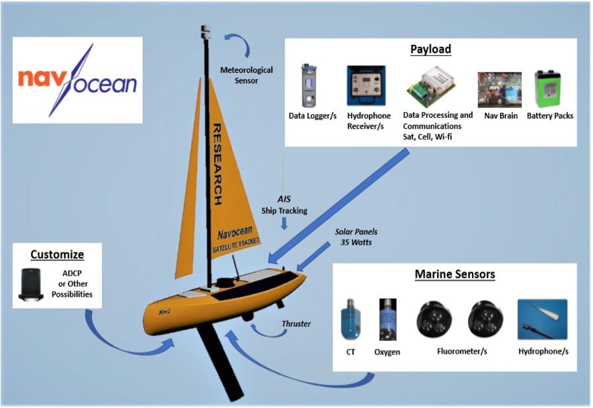
Figure 1. Diagram of the Navocean Nav2 Autonomous Sail Vehicle and components.

TABLE 1

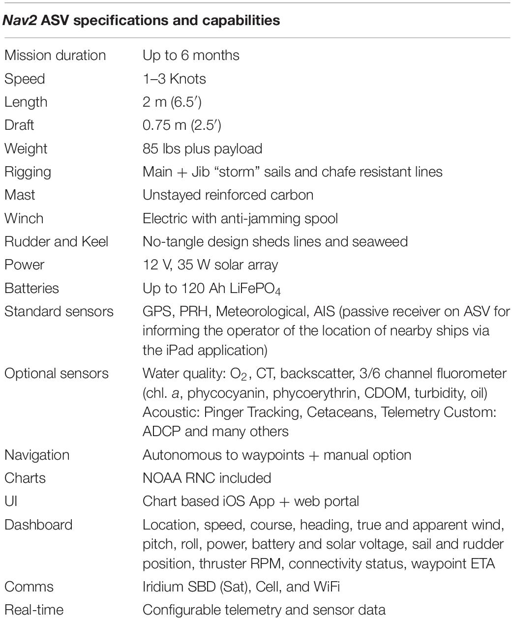
Table 1. Specifications for the Nav2 Autonomous Sail Vehicle (Navocean).

FIGURE 2

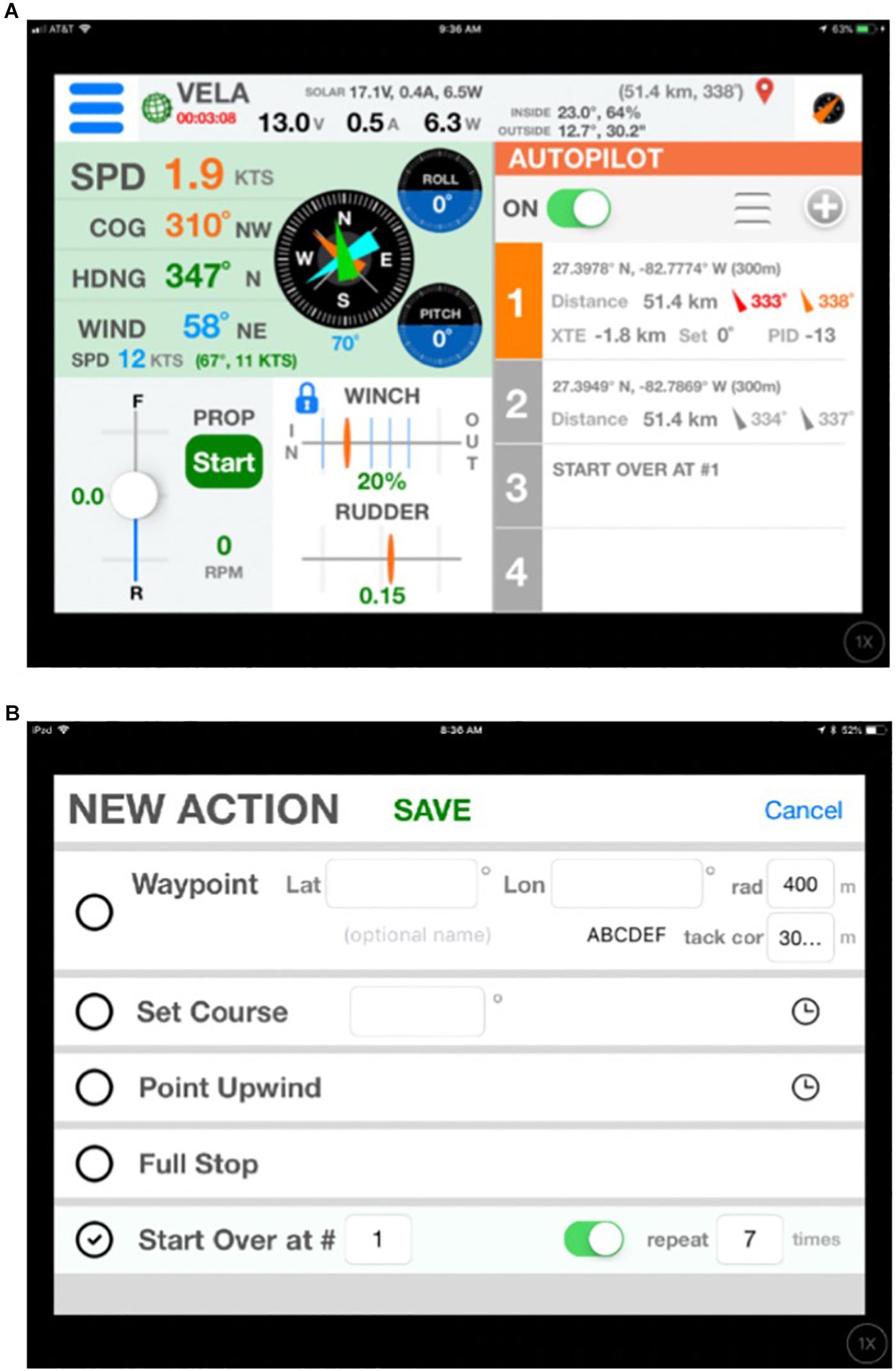
Figure 2. Screenshots of the iOS control software running on an iPad, illustrating operation via Manual Control (A) or via Waypoint navigation (B).

A three-channel fluorometer (Turner Designs Cyclops Integrator/C3) configured for measurement of chlorophyll a (Excitation 465 nm/Emission 696 nm), colored dissolved organic matter (CDOM; measured via fluorescence proxy at 325/470 nm), and turbidity (backscatter at 850 nm) was installed in the hull, behind the main keel, facing downward. The chl. a and turbidity channels underwent single-point linear cross-calibration in the laboratory using ultrapure deionized water and a natural estuarine surface grab sample from Sarasota Bay. The reference measurement was made with a Turner-7F fluorometer operating at the same wavelengths as the sailboat sensor (the surface bottle sample had a turbidity of 0.48 NTU and 0.58 μg L^–1 chl. a). The CDOM channel was calibrated using the same surface bottle sample, but first filtered (0.2 μm). As the CDOM fluorometric measurement is a relative index of CDOM concentration and not a true absorption measurement, the response from the CDOM channel was operationally calibrated based on relationships to CDOM absorption at 440 nm measured on field samples in the laboratory (the surface bottle sample a₄₄₀ was 0.127 m^–1).

Assessment

Vehicle Performance

For the HAB monitoring trials, the Nav2 vehicle was deployed from the beach three times between December 18, 2017 and February 7, 2018, for deployments of increasing length of 1, 3, and 7 days (Table 2 and Figure 3), in which case the boat traveled a total of 254 nautical miles (i.e., 470 km; 1 NM = 1.9 km) at an average rate of 1.0 knots (1 knot = 1 NM h^–1). Winds were relatively low during this time period, corresponding to an overall average of 6.3 knots as compared to average monthly December and January magnitudes of 10–13 knots¹.

TABLE 2

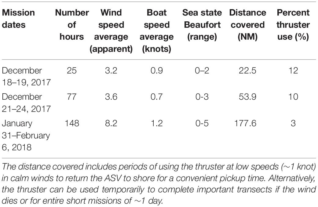
Table 2. Summary of the environmental conditions and the Nav2 ASV performance during harmful algae bloom tracking deployments.

FIGURE 3

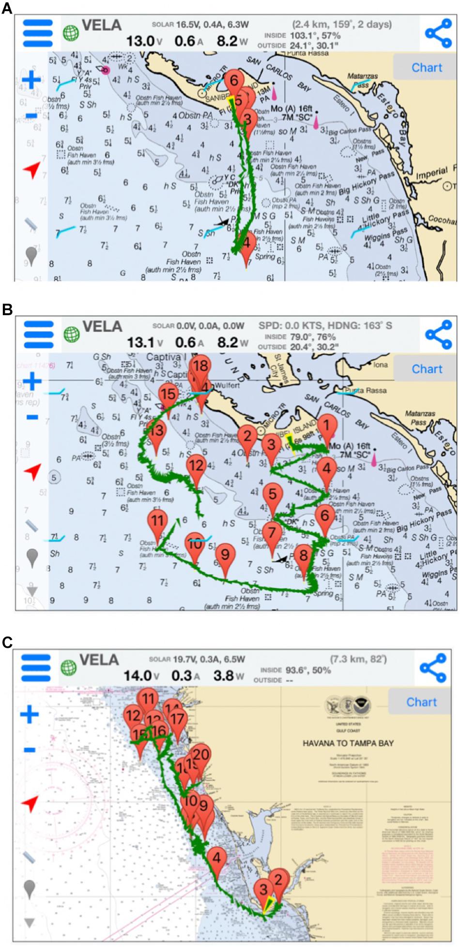
Figure 3. Screenshots of the iOS control software running on an iPad, illustrating the three ASV tracks in southwest Florida for the purposes of harmful algal bloom monitoring from deployments between (A) December 18 and 19, 2017, (B) December 20 and 23, 2017, and (C) January 31 and February 6, 2018.

Each mission was operated in a similar manner. The initial waypoints were entered in advance via WiFi using the chart-based app. Iridium satellite communication was used after deployment to monitor the vehicle’s progress and send updated waypoints as desired, but all navigation was controlled autonomously. To start each mission, the Nav2 was deployed from Sanibel Beach by hand rolling the ASV on its cart out to a depth of >0.75 m, pointing it offshore, and providing a mild push. At the end of each mission, the Nav2 was directed to sail straight to shore until the keel grounded in shallow water. The Nav2 was then placed back onto the wheel cart and pulled on-shore. For the 25-h deployment beginning 2040 UTC December 18, 2017 (Figure 3A), the Nav2 was directed to head straight out and back; sailing first nearly due south to a point 10 NM offshore and then returning north to the beach. On the way back, in response to very calm winds, the thruster was turned on at minimal power to provide a speed of 1 knot, which was enough to reach shore at a convenient time for pick-up. Some drift was caused by local currents, which presents as a bend in the transect line. Despite the boat experiencing a near full tidal cycle in both the southward and northward direction of travel and experiencing winds between 0 and 3 knots for most of the deployment, the Nav2 steadily progressed. This first short mission served as a data collection test of the fluorometer, which was logging to an SD card on board. For the 77-h deployment beginning 1422 UTC December 20, 2017 (Figure 3B), the Nav2 was again deployed directly from Sanibel Beach. The intent of this mission was to sail through an area with a known HABs bloom. The Nav2 was directed to first travel south in a zig-zag pattern to cover increased area compared to the first deployment. In response to updated satellite imagery, the Nav2 was then directed west 15 NM and then north returning to a convenient pick up location at the NE limits of Sanibel Island. The decision was made to persist with sail power for nearly the entire mission to better assess performance in the very calm wind conditions. Depending on solar gain and battery status, the thruster can be used for up to 48 + continuous hours to complete straight transects in a timely manner. Tidal current drift effected the precision of transect lines when the wind was <3 knots. The vessel was removed from the water mid-deployment by a recreational boater, who mistakenly assumed the vessel was lost, and who then traveled with the Nav2 in a northwest direction for 5 km. The Nav2 was tracked during this time and contact was established with the recreational boaters, who were instructed to place the vessel back into the water. At the end of this mission, a more prominent statement was added to the Nav2’s sail, indicating boldly its nature as a tracked and monitored research vessel. No such problem has occurred since. Near the end of the mission, the winds were calm and the thruster was used at low power to return in a timely manner for pickup at the beach. For the 148-h deployment beginning1841 UTC January 31, 2018 (Figure 3C), the vessel was again deployed from Sanibel Beach with the intent of traversing a significant distance of the West Florida Shelf. The vessel traveled west around Sanibel Island and then proceeded northward along the coast between 10 and 30 km offshore. After approaching Tampa Bay, the Nav2 was given waypoints to perform several longitudinal transects, until eventually being directed to the south for retrieval at Venice Beach.

To evaluate the sailing capabilities of the Nav2 vessel, a polar diagram was constructed (Figure 4). The diagram illustrates the obtained vessel speed as a function of realized apparent winds as sensed by the onboard wind sensor (Figure 1). For winds from angles directly behind the vessel to as far as 45° into the wind while under waypoint navigation, the vessel autonomously steers directly to the desired destination and the colored lines represent Velocity Made good on Course (VMC). If the Nav2 is traveling toward a desired waypoint that happens to be directly into the wind (with a threshold of 45° port or starboard), the vessel instead autonomously chooses to tack and achieves a net Velocity Made Good (VMG) toward the waypoint. Represented in Figure 4 are therefore two separate calculations; if winds are < 45° off of the bow, the VMG instead represents the apparent velocity with respect to the destination. Increasing apparent wind velocities results in higher Nav2 velocities for speeds at least as high as 25 knots, under which conditions the vessel is capable of traveling at average speeds >2 knots. The Nav2 is capable of reaching average speeds >1 knot if winds are at least 5–10 knots and greater than 60° away from the wind. Under low wind conditions <5 knots, the vessel realizes VMC/VMG > 0.5 knots for all apparent wind directions >30°. Overall, the vessel is capable of realizing significant forward progress, regardless of wind direction, in all but the most unfavorable wind conditions (>40 km day^–1).

FIGURE 4

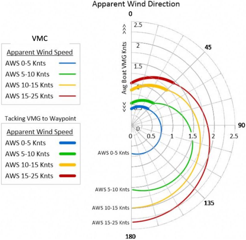
Figure 4. A polar diagram illustrating averaged Nav2 velocity magnitude while sailing as a function of apparent wind magnitude and direction for all deployments. The four colors represent data for intervals for binned wind speeds. Between angles of 45° and 180°, the magnitude is the actual realized velocity over ground of the vehicle in the intended direction, or the “Velocity Made Good on Course.” The Nav2 tracks as does a traditional sailboat at wind angles <45°, realizing VMG (“Velocity Made Good”), and the vessel makes significant forward progress even when traveling at very low angles relative to the wind.

To evaluate if there were effects of bubbles on the fluorometric data, the three measured parameters were binned according to the wind speed at the time of data collection (Figure 5). We are assuming in this case that higher wind speeds would generate more choppy ocean conditions and thus a larger number of bubbles that may provide measurement artifacts both attenuating and amplifying signals, depending on several factors. However, we observe that the fluorometric data do not appear to depend on wind speed. While there is an increase in chl. a values at lower apparent wind speeds, this is likely just coincident with the Nav2 experiencing lower winds closer to shore in the first two deployments, in the presence of the confirmed algae bloom (described in the next section).

FIGURE 5

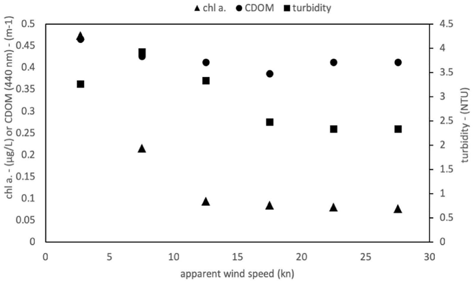
Figure 5. For all deployments, the fluorometer data were binned by their associated 5-knot interval apparent winds speeds to determine if wind and associated bubbles exhibited an artifact.

Harmful Algal Bloom and Environmental Monitoring

To explore the utility of the Nav2 as a platform for HAB detection and mapping, the chl. a fluorometer was used as a semi-quantitative proxy for algal presence. The CDOM and turbidity channels provide additional insights into particulate densities and environmental conditions. These results are placed in the context of ancillary/confirmatory low spatial resolution water sampling and satellite remote sensing measurements. Sentinel-3A level-1 data were acquired from the European Space Agency web portal² and processed to level 2 using NASA’s SeaDAS package (version 7.5). Satellite chlorophyll and spectral remote sensing reflectance image data were extracted from Nav2 GPS matchup positions. Two individual images from December 17, 2017 and February 1, 2018 were used to generate matchups for the three tracks. In this case, the two Nav2 segments from December (December 19–24) were applied to December 17, 2017, and the track data from January 31 to February 6 were applied to the February 1 image.

For the first two, shorter deployments, a large and intense K. brevis (Florida Red Tide) bloom was present nearshore (∼2 km) toward which the vessel was directed (Figures 6A,B). These deployments simulate a potential mission to map spatial HAB bloom patterns in localized areas in response to a bloom, perhaps to guide adaptive sampling, generate semi-quantitative spatial maps and locate hotspots, and determine bloom heterogeneity (i.e., patchiness). The third deployment of 1-week duration on the other hand was intended to demonstrate the potential for the boat to be used for sustained, large-area monitoring, perhaps in a situation where no known blooms are expected, even in off-shore environments (Figure 6C). Generally, the spatial trends of the in situ fluorometric data were consistent with results from water samples and satellite imagery (Figure 7). Elevated chl. a south/southwest of Sanibel Island was probably due primarily to K. brevis, given that this species was identified locally at >10⁶ cells L^–1 (discrete samples in Figures 6A–C). However, chl. a concentrations derived via remote sensing (see color bars in Figure 6 and satellite matchups in Figures 7D–F) were significantly higher than the in situ fluorometer data (∼10×). In situ measurements also revealed more bloom heterogeneity than did the satellite data.

FIGURE 6

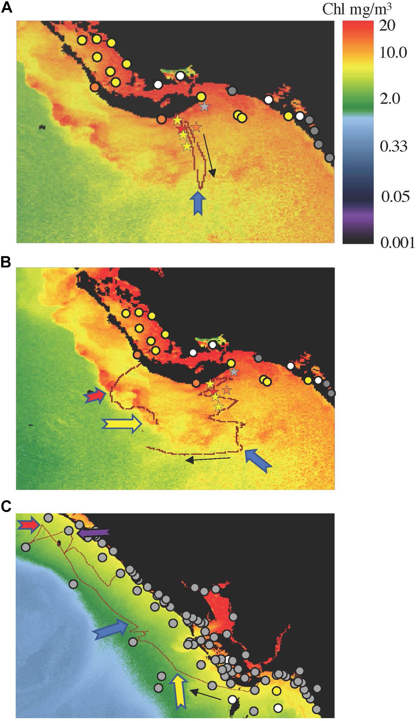
Figure 6. Nav2 deployment tracks (red line) overlain upon Sentinel3A OLCI satellite imagery, as well as enumerated K. brevis cell count data from the Florida Fish and Wildlife Commission (circles) and the Sanibel-Captiva Conservation Foundation (stars). A satellite track image from December 17, 2019 is used to represent the December 18–19, 2017 (A) and December 20–23, 2017 track (B), while the January 31–February 6, 2018 track is on an image from February 2, 2018 (C). The black arrows indicate the direction of the Nav2 track, and the colored block arrows indicate specific locations in the transect that correspond to those in the time-series data in Figure 7. Discrete samples collected and enumerated for K. brevis cells are within 1 week of the deployment in (A,B) but 1 month of the deployment in (C) as sampling was less intense because the major bloom temporarily dissipated. Gray indicates not present/background levels, white indicates very low densities >1,000–10,000 cells L^–1, yellow indicates low densities 10,000–100,000 cells L^–1, orange indicates medium densities 100,000–1,000,000 cells L^–1, and red indicates high >1,000,000 cells L^–1.

FIGURE 7

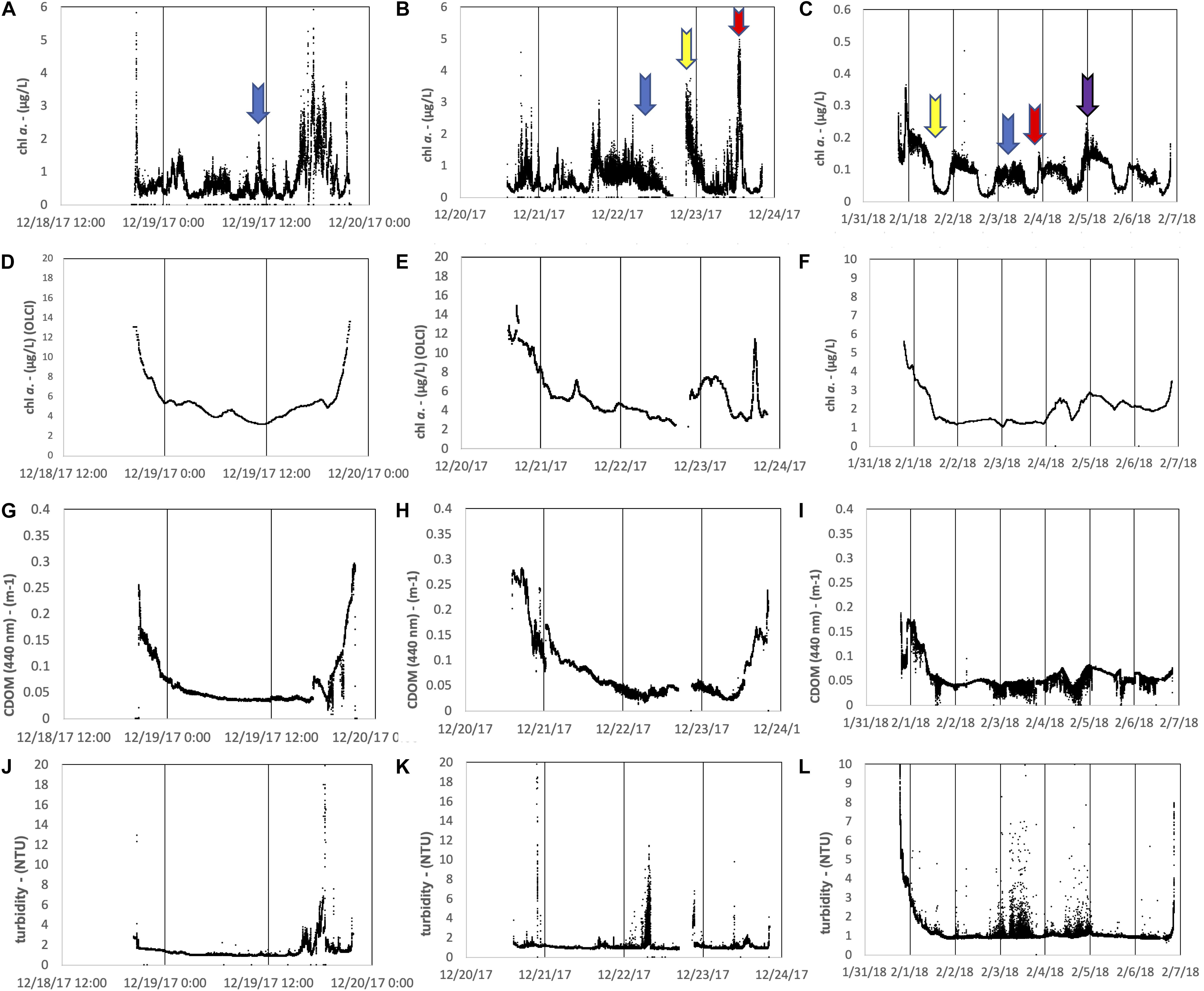
Figure 7. For the December 18–19, 2017, December 20–23, 2017, and January 31–February 6, 2018 deployments, the Nav2 fluorometrically measured chl. a time series is represented in (A–C) respectively, Sentinel3A OLCI satellite chl. a is measured in (D–F), CDOM measured via fluorometric proxy is represented in (G–I), and turbidity is represented in (J–L). Note that the y-axis magnitudes are different for the January 31–February 6, 2018 deployment.

For the first deployment between December 18 and 19, 2017 (Figure 6A), the vessel encountered an elevated chl. a patch immediately south of the beach deployment location. Peak in situ concentrations in the patch were ∼6 μg L^–1 but were more typically between 1 and 3 μg L^–1. Interestingly, the initial Nav2 transect (i.e., southward) only recorded chl. a concentrations less than 1.5 μg L^–1, illustrating the heterogeneity within the patch. In contrast, the remotely sensed background patch was larger and concentrations were higher, between 5 and 20 μg L^–1. The second deployment between December 20 and 23, 2017, again revealed a high degree of spatial heterogeneity. For the first portion of the deployment, chl. a concentrations rarely exceeded 2 μg L^–1. After traveling further west, the vessel soon encountered two chl. a patches greater than 5 μg L^–1, consistent with a concentrated bloom on the SW end of Sanibel observable via satellite (Figure 6B), which also illustrated a patchy distribution. For the final deployment beginning 5 weeks later, between January 31 and February 6, 2018, in situ chl. a values were an order of magnitude lower than in December 2017. Just south of Sanibel Island, chl. a approached as high as 0.4 μg L^–1, but then remained less than 0.2 μg L^–1 for most of the remainder of the deployment. The higher values are consistent with the vessel being closer to shore, but also probably also with the residual bloom, as K. brevis cell counts were still detectable at very low concentrations to the west of the deployment location. Indeed, routine monitoring grab samples did not indicate the presence of K. brevis. While satellite chl. a was again much greater than the in situ Nav2 data, its relative magnitude also decreased by approximately an order of magnitude, with concentrations ∼5 μg L^–1 nearshore and less than 2 μg L^–1 for the offshore portion of the deployment. Interestingly, several portions of the color track show conspicuously less chl. a when unexpected, such as traveling parallel to shore along an isobath. Upon further investigation, this phenomenon was revealed to be the result of diel variations (Figure 8C). Very distinct depressions of the chl. a signal were observed between the daylight hours of 1300 and 2300 UTC (8:00 am and 6:00 pm locally). These variations are likely explainable by vertical diel migration (Happey-Wood, 1976) or by variations in pigment expression, quenching, or measurement artifacts (Babin et al., 1996). These intraday variations were not observed in other deployments where K. brevis was likely present (i.e., patchy, elevated chlorophyll in Figures 8A,B), or during the very first day of the 2018 deployment (most elevated chl. a values in Figure 7A near the probable K. brevis, consistent with the knowledge that this organism does not migrate downward during the day) (Schofield et al., 2006).

FIGURE 8

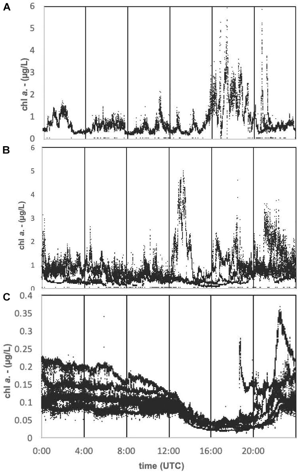
Figure 8. To examine diel trends, daily time series for chl. a are presented for the (A) December 18–19, 2017, (B) December 20–23, 2017, and (C) January 31–February 6, 2018 deployments. Multiple days are depicted on the same plots. Note that the y-axis magnitudes are different for the January 31–February 6, 2018 deployment.

Turbidity and CDOM data provide further information regarding the environmental context of these organisms (Figures 7G–L), as well as evidence for the proper functioning of the Nav2/fluorometer package, i.e., that the data are consistent with expectations. The CDOM data are represented as absorption at 440 nm despite being fluorometrically obtained. While this is not traditional, we argue that an estimation of CDOM absorption is arguably more useful than representing data in more traditional units (e.g., quinine-sulfate units), and a linear response would be expected either way. Thus, while the CDOM magnitude may not be completely accurate (although values between 0.05 and 0.3 m^–1 are consistent with CDOM data measured at the Caloosahatchee River outflow) (Del Castillo et al., 2000), the spatial variance in the observed CDOM should in fact be accurate. For all three deployments, CDOM increased nearshore, consistent with freshwater discharge from inlets, both at deployment and retrieval sites but also during mid-deployment transects (e.g., February 2, 2018; Figure 7I). Other increases appear associated with K. brevis patches (based on the chl. a signature) or river plumes (e.g., December 19, 2017; Figure 7G).

Along these lines, in the absence of a bloom and in a coastline receiving discharge from a single freshwater source, the CDOM data may serve as a rough proxy for salinity (although the presence of CDOM-generating HABs may affect accuracy). Turbidity, being measured as the amount of light scattered at 90° from a source at a single wavelength, appears to more reflect a combination of suspended sediment and phytoplankton cells (Figures 7J–L). Turbidity measurements were more transient and less precise at a single location than CDOM (e.g., February 3 and 4, 2018; Figure 7L), consistent with transient suspended sediments and a heterogeneous water column. Winds were indeed in the 12- to 25-knot range on February 3 from around UTC 0600 to 2200, and then periodically elevated on February 4 throughout the day, which may provide an explanation for these observations. Turbidity increases were also observed near K. brevis bloom patches (evidenced by elevated chl. a; Figure 7J). It is notable that CDOM measurements have a higher precision than the turbidity measurements (e.g., Figures 7I,L). This is expected because the dissolved CDOM will be much more homogenously mixed than will particulates measured via turbidity.

Interestingly, the Sentinel3 OLCI satellite matchup data (Figures 7D–F) matched much more closely with Nav2 CDOM measured in situ with the fluorometer (Figures 7G–I) than it did with either chl. a or turbidity Nav2 measurements. Correlation coefficients between OCLI CDOM and Nav2 CDOM were between 0.65 and 0.39 (Table 3), with the strength of the correlation decreasing with increasing mission duration, probably an analytical artifact because a single satellite image corresponding to a single day was compared to multiple-day Nav2 missions.

TABLE 3

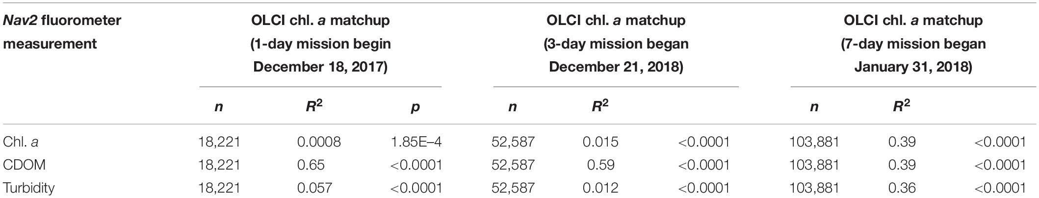
Table 3. Sentinel3 satellite (OLCI) chl. a data matchup statistics revealed from linear regression analysis when correlated to each of the parameters measured using in situ fluorometry by the Nav2 boat.

Discussion

Platform Functionality

Though three deployments of increasing duration, the Nav2 autonomous sail vehicle successfully demonstrated the potential for the platform to provide mobile, unattended monitoring of the surface coastal ocean. The Nav2 is a unique platform in that it is small enough to be deployed in coastal and inland waters, and by functioning identically to a real sailboat, it can obtain high speeds relative to most other autonomous ocean-going platforms and accurately navigate and map areas of interest. The deployments demonstrated that the vessel is robust enough to reliably operate and survey under non-ideal sea states with winds up to 25 knots (although we have tested the vehicle in winds >30 knots in coastal waters of New England and Washington State and more recently > 40 knots on the east coast of Florida, unpublished). Under conditions encountered in southwest Florida with winds averaging less than 4 knots, however, the boat still managed to cover 17–22 NM per day, and 29 NM per day with winds averaging eight knots (Table 2). These winds were not necessarily directed from behind the boat; indeed, the vessel can sail into the wind via autonomous tacking, under which significant forward progress is still made at a VMG of 10 NM per day (Figure 4). The vessel is capable of efficiently reaching preselected (or adjusted on the fly) waypoints (Figures 2, 3). On the other hand, during deployment and retrieval, the boat can be operated manually in sailing mode, or with a thruster (Table 2). The thruster is particularly useful in areas of high currents or ship traffic. Using the thruster only, the Nav2 can be used for short missions (up to 48 h) without the sail. The thruster is manually operated by the user depending on vehicle performance under sail propulsion.

We demonstrated deployments of up to 1 week. The vessel was operating exceptionally at the time of retrieval and could have continued longer. Indeed, Nav2 deployments since the time of writing this report have lasted for 15 + days. Power efficiency improvements are ongoing with multi-sensor, multi-month mission lengths feasible. Approximately 1–5 W extra power is available for sensors. The power availability and length of mission will vary with solar conditions. In solar conditions typical of Florida, the panels typically provide an average of 200 W h day^–1. In low-light conditions typical of northern latitudes in the winter, mission planning needs to be adjusted accordingly.

Deployment or retrieval of the Nav2 is simple but exciting and can be achieved from a boat ramp or from the beach under calm seas by a single operator. All three deployments described herein were initiated from the beach. For deployment, the operator simply walks the small hand-held trailer into the surf zone into waist-deep water until it is floating, and then slides the trailer out from underneath the vessel. The operator can leave the iOS device on shore during the actual deployment or place it into a waterproof case and hold with a lanyard. For retrieval, the vehicle can be lifted back onto its wheel cart by hand in shallow water and then pulled on shore. The Nav2 is also capable of being lifted from the water directly from a small boat. An easily overlooked aspect of using the vehicle is the attention that it garners from beachgoers. This is an opportunity for community outreach, and the southwest Florida HAB monitoring deployments were met with great inquiry and enthusiasm, eventually becoming the subject of several media features. Unfortunately, however, this curiosity also led to mission interruption on December 22, 2017, when a recreational boater pulled the Nav2 from the water and proceeded toward shore until seeing the contact information and statement on the ASV. Under extremely low winds, if the vessel is not obviously making forward progress, it can appear “lost.” Of course, theft is always an issue, especially of a smaller 2-m-long boat. Future versions of the vehicle are expected to be slightly larger to hold a larger number of sensors; this may also serve the dual purpose of being a theft deterrent. The “curiosity” effect has been better managed since these deployments by adding a large bold statement directly on the sail indicating the Nav2 is a “RESEARCH VESSEL” “TRACKED AND MONITORED AT ALL TIMES.” Boaters are increasingly aware that drones of all types on land or sea are carefully monitored. No problems with curiosity or theft have occurred since. Other ongoing improvements with the Nav2 vehicle include an increased vehicle size to more easily accommodate a variety of sensors, the integration and testing of additional sensors, refinements to the autonomous steering algorithm to reduce oversteering and increase average speed, improved consistency of performing desirable straight data collection transects in variable currents, and improved power efficiency to provide greater power for sensors and in low-light conditions.

Applications for Marine HAB Monitoring

The utility of the platform was demonstrated for the specific application of harmful algal bloom monitoring of the Florida Red Tide species K. brevis. The recurring K. brevis blooms ravaging southwest Florida are challenging to monitor because blooms are most detrimental nearshore but in many cases are transported shoreward from deeper waters (Vargo, 2009). Depth-resolved measurements are ideal and have been routinely obtained with AUV buoyancy gliders as part of the State of Florida monitoring program. These deployments have provided extremely valuable insights into waters >10 m deep. In shallower systems, however, gliders progress slowly horizontally, especially in physically dynamic environments. Gliders are also more expensive to operate in shallow waters (they require more frequent attention and battery and buoyancy pump servicing), prohibiting continuous operation. Finally, gliders possess a limited selection of sensors and face many sensor design constraints especially when fluidics are involved (as buoyancy is affected), currently limiting the wide use of species-level detection techniques. Regardless, by the time K. brevis blooms approach the coast within a few kilometers, they are usually at the surface of a well-mixed water column and the need for depth-resolved measurements is decreased (Robbins et al., 2006). Thus, there will, for the foreseeable future, be a niche that must be filled for sustained coastal surface monitoring for this species.

The work presented herein used a fluorometric chl. a sensor, which has since 2015 been the primary sensor employed on Slocum buoyancy gliders for K. brevis monitoring by the State of Florida. The success of the platform/sensor combination for monitoring K. brevis and in generating high-quality fluorometric data is demonstrated by good relationships between water sample K. brevis cell counts (i.e., highest chl. a measured nearshore and to the SW in Figures 6, 7), good matchup to satellite remotely sensed chl. a in the areas with the most intense blooms (i.e., nearshore in Figure 6A and to the west in Figure 6B), repeatable diel variations (Figure 8C), high resolution of bloom “patchiness” (Figures 7A–C), obtainment of reasonable ancillary fluorometric data (Figures 7G–L), and a lack of discernible bubble artifacts (Figure 5). The reproducible diel Nav2 chl. a variations during the 7-day mission in which the vessel encountered Beaufort sea states as high as 5 suggest that bubbles are not an issue (Figure 8). Overall, the excellent time resolution and reproducibility (i.e., Figure 8C) of the measurements highlight the appropriateness of the platform for use in surface water quality monitoring when employing a fluorometric sensor.

Interestingly, the chl. a data obtained in situ were of much lower concentration than those detected by satellite. These variations are expected based on the very different nature of the measurements. Satellite measurements integrate over a depth interval and calculated concentrations are therefore representative of an average concentration of the surface water column. Fluorometric chl. a is only considered to be semi-quantitative, so absolute chl. a concentrations are probably not as informative as spatial variations. In situ chl. a measurements reveal much greater spatial variability than the satellite measurements, consistent with our knowledge of K. brevis in which cell concentrations can easily vary by an order of magnitude just a few meters from each other. Satellite measurements are also more challenging in turbid and CDOM-rich optically complex waters where we conducted the deployments. Indeed, the far greater correlation between Nav2 chl. a and OLCI CDOM (Table 3) is sensible in this context. Indeed, certain regional correction algorithms have been demonstrated to be more accurate for determining the presence of K. brevis, and these may be evaluated in the future (Hu et al., 2005). Overall, however, results serve as justification for the investment into compatible HAB species-specific sensors and satellite algorithms.

An unexpected result was the repeatable diel variations observed during the longer mission (Figure 8C). Fluorometric measurements of chl. a can be subject to solar-induced photoinhibition (e.g., Kiefer, 1973), various packaging effects, and fluorescence quenching, especially at higher concentrations. Numerous accessory pigments can also contribute to the signal (Babin et al., 1996; Schofield et al., 2006). Similar results are routinely observed on the West Florida Shelf during multi-day, routine glider missions in which no K. brevis is present based on cell counts (example datasets are available in the GCOOS repository)³. K. brevis cells exhibit positive phototaxis migratory behavior during the daylight hours, which may increase the fluorescence signature (Schofield et al., 2006). K. brevis blooms also typically dominate the taxa when present and exhibit extreme small-scale spatial variability. We therefore propose that in this geographic region subject to frequent K. brevis blooms, elevated and patchy chl. a patterns like those in Figures 8A,B that far exceed a background diel signature (i.e., Figure 8C) can be used as a potential signature for K. brevis. While the presence of the organism would of course need to be verified, the Nav2 dataset could, in this fashion, be used to guide adaptive sampling. With a fleet of Nav2 vehicles traveling ∼20 NM per day in a repeatable triangular or “lawnmower” raster pattern, several vehicles have the potential to continuously survey a large area, regardless of water depth. The Nav2 equipped with a fluorometer, while perhaps not as accurate at a species level as satellite remote sensing using the most current and optimal algorithms, can reveal K. brevis surface heterogeneity at a high spatial resolution once a bloom has been confirmed.

Other Monitoring Applications

While chl. a measurements were the primary focus of this project, the ancillary fluorometric data streams also shed light on some in-water processes and allude to future applications of the Nav2 vessel. The fluorescence response of organic matter has been extensively used as a proxy since terrestrially based coastal CDOM can, for discrete regions and time intervals, display nearly linear relationships with salinity and FDOM (Coble, 1996; Del Castillo et al., 2000). CDOM is of interest to biogeochemists for its role in dominating ocean color, playing a critical role in photobiology, photochemistry (Helms et al., 2008), and photoproduction of CO₂ (Clark et al., 2004), contributing to aspects of the oceanic sulfur cycle (Gali et al., 2016), and controlling the absorption of light energy and the subsequent impacts on heat flux (Hill, 2008) and other ocean–climate interactions, and in serving as a tracer of freshwater (Fichot and Benner, 2012). The fluorometrically measured CDOM exhibited intensities and spatial concentration distributions that are expected in southwest Florida (Del Castillo et al., 2000). Earlier in the project, we did install a conductivity-temperature-depth CTD package onto the vehicle. However, conductivity measurements were unreasonable, perhaps because the CTD was configured immediately behind the rudder in an area where bubble creation is visibly intense. While we still aim to resolve this issue with a different installation configuration, it is worth considering the use of CDOM as a rough proxy for salinity, with the assumption that there is a single source of freshwater input that has a high CDOM concentration (i.e., the Charlotte Harbor and the Caloosahatchee River). The use of CDOM as a rough proxy for salinity has been well demonstrated by several research groups and is one of the primary means to estimate salinity from remote sensing as long as the regional proxy is well defined and the inputs into the system are known (Bowers and Brett, 2008; Del Castillo and Miller, 2008).

The Nav2 is inherently a meteorological sensor (e.g., for wind speed and magnitude, atmospheric temperature, and humidity). Previously, the Nav2 has been successfully configured with fisheries sensors, including a pinger tracking hydrophone system (Sonotronics) and a cetacean and noise monitoring hydrophone (Song Meter). Trials demonstrated successful location of crab tracking pingers on the Washington coast and acoustic detection of various cetacean species. As of the time of writing, we are currently adding a Wetlabs BB3 Scatterometer and a Solinst CT logger for HABs surveys on Lake Okeechobee and the Indian River Lagoon in Florida. Addition of Oxygen/Temp Optode (Aanderaa AADI) and CT sensors as well as an ADCP (Nortec) are under consideration to provide a complete water quality monitoring suite.

Conclusion

The Navocean autonomous sail vehicle (Nav2) has been demonstrated to serve as a reliable mobile platform for wide-area surface coastal monitoring. To our knowledge, this is the first demonstration of a sail-driven vessel used for coastal HAB monitoring. The scientific results were shown to be reasonable and demonstrate the potential for mapping unispecies HAB blooms and guiding adaptive sampling, while simultaneously collecting important environmental data. While the Nav2 does not capture depth variations or collect instantaneous large surface area measurements as do underwater gliders and satellites, respectively, the platform is a useful tool in a larger arsenal for coastal or inland monitoring. The primary benefits of using the Nav2 vehicle are that it is fast and has reliable, autonomous navigation, has a completely renewable power source with no consumables, can function in shallow or deep water inland or offshore, and is operable by a single person. There are several additional demonstrated payload options as well as some currently in preparation. At least with the planar-style optical sensors, bubbles do not appear to contribute significant artifacts.

Harmful cyanobacterial blooms are also increasing in intensity in global freshwater bodies (Paerl et al., 2018). The Nav2 vehicle is ideal for monitoring blooms in these frequently shallow lakes, especially by limnologists who may have less training with more traditional oceanographic tools. To this end, we have recently deployed the Nav2 for freshwater M. aeruginosa HAB monitoring in Lake Okeechobee in February 2019. A second three-channel fluorometer was installed to provide phycocyanin and phycoerythrin measurements that help discriminate multiple algal species. The deployment garnered press from at least eight news outlets and the vehicle successfully navigated a series of transects in the lake (available on GCOOS Gandalf, 2019 data archive). Until the summer of 2018, there were few traditional monitoring efforts and no real-time water quality monitoring sensors on Lake Okeechobee, and even now, only one stationary optical sensor is providing ground-truthing data for satellite efforts. We plan in the future to augment this fixed location monitoring with Nav2 surveys to both add a mobile monitoring element and constrain the spatial variability of the surface optical properties in relation to remote sensing data. Ultimately, we envision the Nav2 platform becoming a critical tool in multiple monitoring programs.

Author Contributions

JB authored the manuscript, provided scientific oversight, and participated in field campaigns. EA was the lead designer of the autonomous vehicle hardware and software. TM performed the satellite matchup validation. BC developed the live data visualization interface. EM coordinated the field campaigns. SD designed the sailboat and conducted the deployments.

Funding

This work was supported in part by a National Academies Gulf Research Program Early-Career Fellowship award #2000007281 that supported salary and supplies, and the Gulf of Mexico Coastal Ocean Observation System #NA16NOS0120018 that supported salaries.

Conflict of Interest

EA and SD were employed by Navocean, Inc.

The remaining authors declare that the research was conducted in the absence of any commercial or financial relationships that could be construed as a potential conflict of interest.

Acknowledgments

We would like to thank L. Kellie Dixon, Jim Hillier, and Karl Henderson at Mote, and last but not least our former high school intern Gabriel Rey for assistance with the field work.

Footnotes

1. ^ https://www.windfinder.com/windstatistics/southwest_of_tampa_bay_buoy
2. ^ https://scihub.copernicus.eu/
3. ^ https://gandalf.gcoos.org/data/gandalf/mote/mote-genie/2016/2016_12_12/plots/

References

Anderson, D. M., Glibert, P. M., and Burkholder, J. M. (2002). Harmful algal blooms and eutrophication: nutrient sources, composition, and consequences. Estuaries 25, 704–726. doi: 10.1007/bf02804901

CrossRef Full Text | Google Scholar

Babin, M., Morel, A., and Gentili, B. (1996). Remote sensing of sea surface sun-induced chlorophyll fluorescence: consequences of natural variations in the optical characteristics of phytoplankton and the quantum yield of chlorophyll a fluorescence. Int. J. Remote Sens. 17, 2417–2448. doi: 10.1080/01431169608948781

CrossRef Full Text | Google Scholar

Backer, L. C., McNeel, S. V., Barber, T., Kirkpatrick, B., Williams, C., Irvin, M., et al. (2010). Recreational exposure to microcystins during algal blooms in two California lakes. Toxicon 55, 909–921. doi: 10.1016/j.toxicon.2009.07.006

PubMed Abstract | CrossRef Full Text | Google Scholar

Bowers, D. G., and Brett, H. L. (2008). The relationship between CDOM and salinity in estuaries: an analytical and graphical solution. J. Mar. Sys. 73, 1–7. doi: 10.1016/j.jmarsys.2007.07.001

CrossRef Full Text | Google Scholar

Bowers, H., and Smith, G. J. (2017). “Sensors for monitoring of harmful algae, cyanobacteria and their toxins,” in Workshop Proceedings, ed. A. F. C. Technologies (Moss Landing, CA: Moss Landing Marine Laboratories).

Google Scholar

Brand, L. E., and Compton, A. (2007). Long-term increase in Karenia brevis abundance along the Southwest Florida coast. Harmful Algae 6, 232–252. doi: 10.1016/j.hal.2006.08.005

PubMed Abstract | CrossRef Full Text | Google Scholar

Carmichael, W. W. (2001). Health effects of toxin-producing cyanobacteria: “The CyanoHABs”. Hum. Ecol. Risk Assess. Int. J. 7, 1393–1407. doi: 10.1080/20018091095087

CrossRef Full Text | Google Scholar

Clark, C. D., Hiscock, W. T., Millero, F. J., Hitchcock, G., Brand, L., Miller, W. L., et al. (2004). CDOM distribution and CO(2) production on the southwest Florida shelf. Mar. Chem. 89, 145–167. doi: 10.1016/j.marchem.2004.02.011

CrossRef Full Text | Google Scholar

Coble, P. G. (1996). Characterization of marine and terrestrial DOM in seawater using excitation emission matrix spectroscopy. Mar. Chem. 51, 325–346. doi: 10.1016/0304-4203(95)00062-3

CrossRef Full Text | Google Scholar

Daniel, T., Manley, J., and Trenaman, N. (2011). The wave glider: enabling a new approach to persistent ocean observation and research. Ocean Dyn. 61, 1509–1520. doi: 10.1007/s10236-011-0408-5

CrossRef Full Text | Google Scholar

Del Castillo, C. E., Gilbes, F., Coble, P. G., and Muller-Karger, F. E. (2000). On the dispersal of riverine colored dissolved organic matter over the West Florida Shelf. Limnol. Oceanogr. 45, 1425–1432. doi: 10.4319/lo.2000.45.6.1425

CrossRef Full Text | Google Scholar

Del Castillo, C. E., and Miller, R. (2008). On the use of ocean color remote sensing to measure the transport of dissolved organic carbon by the Mississippi River Plume. Remote Sens. Environ. 112, 836–844. doi: 10.1016/j.rse.2007.06.015

CrossRef Full Text | Google Scholar

Ducharme, J. (2018). Red tide is killing marine life and scaring away tourists in Florida. Here’s what to know about it Time Magazine Online. doi: 10.1016/j.rse.2007.06.015

CrossRef Full Text | Google Scholar

Fichot, C. G., and Benner, R. (2012). The spectral slope coefficient of chromophoric dissolved organic matter (S275–295) as a tracer of terrigenous dissolved organic carbon in river-influenced ocean margins. Limnol. Oceanogr. 57, 1453–1466. doi: 10.4319/lo.2012.57.5.1453

CrossRef Full Text | Google Scholar

Fleming, L. E., Rivero, C., Burns, J., Williams, C., Bean, J. A., Shea, K. A., et al. (2002). Blue green algal (cyanobacterial) toxins, surface drinking water, and liver cancer in Florida. Harmful Algae 1, 157–168. doi: 10.1016/s1568-9883(02)00026-4

CrossRef Full Text | Google Scholar

Gali, M., Kieber, D. J., Romera-Castillo, C., Kinsey, J. D., Devred, E., Perez, G. L., et al. (2016). CDOM sources and photobleaching control quantum yields for oceanic DMS photolysis. Environ. Sci. Technol. 50, 13361–13370. doi: 10.1021/acs.est.6b04278

PubMed Abstract | CrossRef Full Text | Google Scholar

GCOOS Gandalf (2019). The Gulf AUV Network and Data Archiving Long-term Storage Facility. https://gandalf.gcoos.org/data/gandalf/mote/mote-genie/2016/2016_12_12/plots/ (accessed June 8, 2019).

Google Scholar

Gannon, D. P., Berens McCabe, E. J., Camilleri, S. A., Gannon, J. G., Brueggen, M. K., Barleycorn, A. A., et al. (2009). Effects of Karenia brevis harmful algal blooms on nearshore fish communities in southwest Florida. Mar. Ecol. Prog. Ser. 378, 171–186. doi: 10.3354/meps07853

CrossRef Full Text | Google Scholar

Happey-Wood, C. M. (1976). Vertical migration patterns in phytoplankton of mixed species composition. Br. Phycol. J. 11, 355–369. doi: 10.1080/00071617600650411

CrossRef Full Text | Google Scholar

Helms, J. R., Stubbins, A., Ritchie, J. D., Minor, E. C., Kieber, D. J., and Mopper, K. (2008). Absorption spectral slopes and slope ratios as indicators of molecular weight, source, and photobleaching of chromophoric dissolved organic matter. Limnol. Oceanogr. 53, 955–969. doi: 10.4319/lo.2008.53.3.0955

CrossRef Full Text | Google Scholar

Hill, V. J. (2008). Impacts of chromophoric dissolved organic material on surface ocean heating in the Chukchi Sea. J. Geophy. Res. Oceans 113:C07024.

Google Scholar

Hoagland, P., Jin, D., Polansky, L. Y., Kirkpatrick, B., Kirkpatrick, G., Fleming, L. E., et al. (2009). The costs of respiratory illnesses arising from Florida Gulf Coast Karenia brevis blooms. Environ. Health Perspect. 117, 1239–1243. doi: 10.1289/ehp.0900645

PubMed Abstract | CrossRef Full Text | Google Scholar

Hu, C., Muller-Karger, F. E., Taylor, C., Carder, K. L., Kelble, C., Johns, E., et al. (2005). Red tide detection and tracing using MODIS fluorescence data: a regional example in SW Florida coastal waters. Remote Sens. Environ. 97, 311–321. doi: 10.1016/j.rse.2005.05.013

CrossRef Full Text | Google Scholar

Kiefer, D. A. (1973). Fluorescence properties of natural phytoplankton populations. Mar. Biol. 22, 263–269. doi: 10.1007/bf00389180

CrossRef Full Text | Google Scholar

Kirkpatrick, B., Fleming, L. E., Backer, L. C., Bean, J. A., Tamer, R., Kirkpatrick, G., et al. (2006). Environmental exposures to Florida red tides: effects on emergency room respiratory diagnoses admissions. Harmful Algae 5, 526–533. doi: 10.1016/j.hal.2005.09.004

PubMed Abstract | CrossRef Full Text | Google Scholar

McCabe, R. M., Hickey, B. M., Kudela, R. M., Lefebvre, K. A., Adams, N. G., Bill, B. D., et al. (2016). An unprecedented coastwide toxic algal bloom linked to anomalous ocean conditions. Geophys. Res. Lett. 43, 10366–10376.

PubMed Abstract | Google Scholar

Mordy, C. W., Cokelet, E. D., De Robertis, A., Jenkins, R., Kuhn, C. E., Lawrence-Slavas, N., et al. (2017). Advances in ecosystem research saildrone surveys of oceanography, fish, and marine mammals in the Bering Sea. Oceanography 30, 113–115.

Google Scholar

O’Neil, J. M., Davis, T. W., Burford, M. A., and Gobler, C. J. (2012). The rise of harmful cyanobacteria blooms: the potential roles of eutrophication and climate change. Harmful Algae 14, 313–334. doi: 10.1016/j.hal.2011.10.027

CrossRef Full Text | Google Scholar

Paerl, H. W., Otten, T. G., and Kudela, R. (2018). Mitigating the expansion of harmful algal blooms across the freshwater-to-marine continuum. Environ. Sci. Technol. 52, 5519–5529. doi: 10.1021/acs.est.7b05950

PubMed Abstract | CrossRef Full Text | Google Scholar

Reich, A., Lazensky, R., Faris, J., Fleming, L. E., Kirkpatrick, B., Watkins, S., et al. (2015). Assessing the impact of shellfish harvesting area closures on neurotoxic shellfish poisoning (NSP) incidence during red tide (Karenia brevis) blooms. Harmful Algae 43, 13–19. doi: 10.1016/j.hal.2014.12.003

CrossRef Full Text | Google Scholar

Robbins, I. C., Kirkpatrick, G. J., Blackwell, S. M., Hillier, J., Knight, C. A., and Moline, M. A. (2006). Improved monitoring of HABs using autonomous underwater vehicles (AUV). Harmful Algae 5, 749–761. doi: 10.1016/j.hal.2006.03.005

CrossRef Full Text | Google Scholar

Schofield, O., Kerfoot, J., Mahoney, K., Moline, M., Oliver, M., Lohrenz, S., et al. (2006). Vertical migration of the toxic dinoflagellate Karenia brevis and the impact on ocean optical properties. J. Geophys. Res. Oceans 111:C06009.

Google Scholar

Scholin, C. A., Gulland, F., Doucette, G. J., Benson, S., Busman, M., Chavez, F. P., et al. (2000). Mortality of sea lions along the central California coast linked to a toxic diatom bloom. Nature 403, 80–84. doi: 10.1038/47481

PubMed Abstract | CrossRef Full Text | Google Scholar

Shapiro, J., Dixon, L. K., Schofield, O. M., Kirkpatrick, B., and Kirkpatrick, G. J. (2015). “Chapter 18—New sensors for ocean observing: The optical phytoplankton discriminator,” in Coastal Ocean Observing Systems, eds Y. Liu, H. Kerkering, and R. H. Weisberg (Boston: Academic Press), 326–350. doi: 10.1016/b978-0-12-802022-7.00018-3

CrossRef Full Text | Google Scholar

Smith, D. R., King, K. W., and Williams, M. R. (2015). What is causing the harmful algal blooms in Lake Erie? J. Soil Water Conserv. 70, 27A–29A. doi: 10.2489/jswc.70.2.27a

CrossRef Full Text | Google Scholar

Stockley, N. D., Sullivan, J. M., Hanisak, D., and McFarland, M. N. (2018). “Using observation networks to examine the impact of Lake Okeechobee discharges on the St. Lucie Estuary, Florida,” in in Proceedings of SPIE Defense + Security, (Bellingham, WA: SPIE), 8.

Google Scholar

Vargo, G. A. (2009). A brief summary of the physiology and ecology of Karenia brevis Davis (G. Hansen and Moestrup comb. nov.) red tides on the West Florida Shelf and of hypotheses posed for their initiation, growth, maintenance, and termination. Harmful Algae 8, 573–584. doi: 10.1016/j.hal.2008.11.002

CrossRef Full Text | Google Scholar