Deep Currents in the Rift Valley of the North Mid-Atlantic Ridge

1. Introduction

Mid-Ocean ridges are regions where tectonic plates spread apart and new seafloor is formed (Baker and German, 2004). They contain most of the hydrothermal vents, which are associated with an important biogeochemical activity (e.g., iron input—Tagliabue et al., 2010; Conway and John, 2014), and host specific ecosystems characterized by a high degree of endemicity (e.g., Van Dover, 1995, 2000; Herring, 2002). The interactions between the abyssal currents and the topography give rise to complex flows, and these regions are associated with a high level of turbulence and mixing (Polzin et al., 1997). The impact of the deep circulation and hydrography on the hydrothermal habitats and the input of geochemical elements in the water column has received growing interest over the last few decades (e.g., Mcduff, 2013). It is admitted that the dynamics and the connectivity of biological habitats are strongly impacted by the currents (e.g., Mullineaux and France, 2013), and that taking into account the submesoscale (0.1–10 km) variability in ocean models can substantially change the patterns of larval dispersion and biogeochemical tracers (Werner et al., 2007; Vic et al., 2018). A few recent studies have investigated the transport of deep-sea larvae using high-resolution realistic modeling, including the high frequency tidal motions, coupled with a Lagrangian particle tracking tool (Vic et al., 2018; Xu et al., 2018). They showed that topographically-constrained flows dominate the patterns of larval dispersal and that topographic features—such as transform faults—can act as barriers. The presence of submesoscale activity and tidally-induced vertical excursion and mixing can help the larvae overcome these obstacles.

These studies did not aim at understanding thoroughly the abyssal dynamics, and numerous aspects remain poorly understood due to the great complexity of abyssal flows and their variability. However, the mean flow and associated upwelling in deep canyons were investigated in the context of mixing and water masses transformation at several locations over the mid-ocean ridges, especially in the Brazil basin (St. Laurent et al., 2001; Thurnherr and Speer, 2003; Thurnherr et al., 2005; Clément et al., 2017) and over the North Mid-Atlantic Ridge (Thurnherr et al., 2002). The currents in these locations present Ekman-like dynamics (e.g., Phillips, 1970; Wunsch, 1970), with the bottom-enhanced mixing over a slope inducing horizontal density gradients that push the flow upslope at depth. However, due to the sparsity of in-situ observations, little is known about the spatial structure of the currents and the variability of the deep circulation, especially in the sub-inertial range. The direct impacts of the (sub-)mesoscale eddies and internal waves on the mean flow in such realistic configuration remain largely unknown as well, while several possible mechanisms have been identified (Holloway and Wang, 2009; Venaille et al., 2011; Grisouard and Bühler, 2012; Xie et al., 2018). For instance, Clément and Thurnherr (2018) recently reported evidence of non-linear interactions between internal waves and the mean flow in a submarine valley, thus showing that these mechanisms could play a significant role in the deep-ocean dynamics.

The North Mid-Atlantic Ridge (MAR) is very representative of the dynamics depicted above. Between the Oceanographer Fracture Zone (near 35°N) and the Azores archipelago (near 38°N), the rift valley hosts three major vent fields (Figure 1): Rainbow (36°14′N, 33°54′W), Lucky Strike (37°18′N, 32°17′W), and Menez-Gwen (37°50′N, 31°31′W), and several other vent sites that were either directly observed or inferred from plume detection (Beaulieu and Szafranski, 2018). Several cruises have been conducted in the region to investigate the dynamics of the vent fields and hydrothermal plumes, as well as the associated ecosystems. The Lucky Strike vent field is one of the most studied site and has been chosen by the European Multi-disciplinary Subsea and water column Observatory (EMSO-Azores) to develop a long-term seafloor observatory deployed in 2010. In this context, the transport of deep-sea larvae from the hydrothermal vent field was investigated using high-resolution numerical modeling by Vic et al. (2018), showing significant transport and impact of the submesoscale dynamics.

FIGURE 1

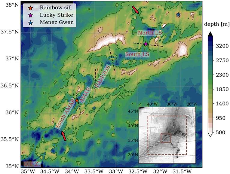
Figure 1. Bathymetry of the North Mid-Atlantic Ridge in the region discussed in this paper (taken from the SRTM30plus database). Black contours indicate iso-depth at 2,000 and 1,000 m. Dashed lines delimitate basins and segments of interest (written in brown). These are usually associated with fracture zones aligned along the West-East direction. The rift valley water is mostly isolated below 2,000 m, except at a few locations: red arrows indicate identified connections (inflows) from the exterior ridge flanks to the inside valley at some of these passages. O.F.Z., Oceanographer Fracture Zone.

The first observations of the hydrography and currents in the rift valley of the MAR date back to Keller et al. (1975) and Fehn et al. (1977), who reported the existence of a northeast mean flow in the FAMOUS channel (near 36°50′N) and a south-to-north density gradient, later confirmed by Saunders and Francis (1985) in several regions of the North Atlantic ridge. Fehn et al. (1977) also reported that the stratification within the rift valley is weaker than over the ridge flank, an observation later confirmed by Wilson et al. (1995, FAZAR cruise) between 33°N and 40°N (with particular emphasis on the Lucky Strike segment), who further inferred the role of enhanced mixing in the region (although considering lateral mixing only). The existence of decreased stratification within the rift valley and up-valley (south-to-north) deep flow associated with a mean density gradient (decreasing upward) have been repeatedly confirmed ever since (Thurnherr and Richards, 2001; Thurnherr et al., 2002, 2008).

Most of the studies mentioned above investigated specific aspects of the deep-ocean dynamics on a local (segment) scale, and were based on observational data. To gain further knowledge on the rift-valley dynamics at a regional scale (from the Oceanographer Fracture Zone up to Menez Gwen hills) as well as its potential implications for transport of biogeochemical species and larvae, we used a high-resolution realistic numerical model to simulate the flow over the North MAR combined with in-situ data gathered from previous surveys. The latter are used to describe the rift-valley flow at a few locations and serve as a basis for evaluating and validating the numerical simulation, while the former offers a more continuous view of the dynamics and allows us to go further in understanding the dynamical aspects of the deep circulation. It also provides some insights on the dynamical forcings and the role of internal tides. All together, these results draw the first description of the deep currents over the scale of the whole rift valley, all the more so using realistic modeling.

The paper is organized as follows. In section 2, we describe the observational datasets and the numerical simulations. A description of the rift valley topography and the mean circulation and hydrography is given in section 3. In section 4 we discuss the variability of the currents together with their dynamical origin. Finally, conclusions are given in section 5.

2. Data and Methods

2.1. Data

We use currents from long-term (typically 1 year) moorings that were deployed near the Rainbow and Lucky-Strike vent fields, providing hourly data. At Rainbow, 7 moorings with 21 current-meters where deployed between the two FLAME cruises (1997–1998, Thurnherr et al., 2002). At Lucky Strike, we use the data from two moorings with two current meters on each, deployed inside the east canyon (see Figure 1) during the Graviluck cruise (2006–2007, Pasquet, 2011; Pasquet et al., 2016) and additional data from ATOS (one current meter between 2001–2002, see Khripounoff et al., 2008) and DIVA (two current meters between 1994–1995, see Jean-Baptiste et al., 1998; Khripounoff et al., 2000) located over the volcano near the segment center (see Figure 1). We also use LADCP data from the Graviluck cruise (Thurnherr et al., 2008).

The hydrographic properties (T, S, and ρ) are estimated using CTD data from several projects: the FLAME experiment (German et al., 1998), FAZAR project in 1992 (Wilson et al., 1995), and HEAT project in 1994 (German et al., 1996), as well as the MOMARdream (in 2007) and Graviluck (Thurnherr et al., 2008) surveys. All CTD data were processed with standard methods and averaged in fixed vertical bins.

2.2. Numerical Modeling

High resolution numerical simulations were done using the Regional Ocean Modeling System (ROMS, Shchepetkin and McWilliams, 2005). The numerical domain is 1,500km wide in both directions, extending between 41.8°W and 23.2°W in longitude, and 30.5°N and 44.2°N in latitude (see inset in Figure 1), with a horizontal resolution dx = 750 m. 80 vertical levels refined near the surface and the seafloor (with corresponding stretching parameters θ_s = 6 and θ_b = 4) are used: the typical vertical resolution in the rift valley ranges between 20 m near the seafloor to 100 m at 2,000 m, over the deepest basins. Data from simulations in a larger domain are prescribed at the boundaries using a one-way nesting approach with two steps: the simulation in the largest domain, extensively described in Gula et al. (2015), covers most of the North-Atlantic ocean and has a horizontal resolution dx = 6 km. The second simulation was used as a buffer with 2 km horizontal resolution and covers a domain slightly larger than the one used here. The bathymetry is taken from the SRTM30plus dataset (Becker et al., 2009), with additional smoothing to limit discretization errors, and KPP parameterization is used for the vertical mixing (Large et al., 1994). Details on the numerical setup are given in Vic et al. (2018).

Three different types of numerical simulations were performed. The first two are “realistic” setups which include surface forcing (heat flux and wind stress) and nesting from the parent simulation prescribed at the boundaries. One of these runs further includes barotropic tidal forcing, which is imposed at the boundaries by interpolating the TPXO7 global inverse model (Egbert and Erofeeva, 2002). Tidal potential, with tidal self-attraction and loading taken from GOT99.2b model, is further added in the domain. The eight dominant tidal components (M2, S2, N2, K2, K1, O1, P1, and Q1) are used. The model is run for 1 year, after an initial-spin up (from the parent nest state) of 2 months. In addition, a third set of numerical simulations were performed with an idealized setup consisting of tide-only forcing with horizontally uniform stratification, starting from a state at rest. Wind stress and surface heat fluxes were deactivated in these runs, as well as the nesting from parent simulation. The stratification corresponds to a mean profile over the numerical domain computed from the monthly-averaged SODA climatology outputs (Carton and Giese, 2008), i.e., the same as taken for the original, largest simulation. This simulation is run over 2 months. In the following, these runs will be referred as the “no-tide” (nest without tidal forcing), “fully-forced” (nest with tidal forcing), and “tide-only” simulations (cf. Table 1).

TABLE 1

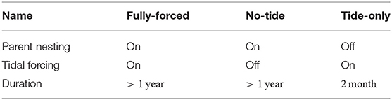
Table 1. Description of the different numerical simulations.

3. Rift Valley, Hydrography, and Circulation: Regional Description

In this section, we describe the topography in the rift valley. We then characterize the mean flow (i.e., over a timescale of a few months to a year) that takes place below 2,000 m, based on observational data and results from the numerical simulation, and finally discuss the density distribution within the rift valley and how it is impacted by this mean circulation.

3.1. Rift Valley Topography

The main bathymetric features of the North Mid-Atlantic Ridge south of the Azores archipelago, which is our region of interest, are illustrated in Figure 1. There is a median valley running along the SW-to-NE-ward trending MAR crest in this region, which is characteristic of slow-spreading ridges. The valley is 500 to 1,000-m deep and several tens of kilometers wide. While individual peaks of the MAR crest extend above 500 m, the rift valley is topographically closed below ≈2,000 m, i.e., the rift-valley water below this depth is largely isolated from the waters over both ridge flanks. The floor of the rift valley is characterized by a sequence of basins and troughs deeper than 3,000 m and separated by topographic structures forming sills and narrows. Most segments are deepest near their ends and have shallower regions near their centers. In the case of the Lucky Strike segment there is an active volcano rising to about 1,700 m in the center of the rift valley and hosting several active hydrothermal vents (magenta star in the figure). Two canyons connecting the North and South basins run on both sides of the volcano. Additional shallow regions are found at lateral discontinuities (transform faults and non-transform discontinuities) of the MAR crest, such as the narrow meridional ridge separating the AMAR from the FAMOUS segment or the Rainbow Ridge/Sill complex separating South AMAR from AMAR and hosting the Rainbow hydrothermal vent field (red star in the figure). On a larger scale the MAR crest in this region is sloping upward northeastward toward the Azores—within the rift valley the main signature of this slope is a tendency of the sills connecting the deeper basins in the valley floor to shallow toward the north.

In the rest of the paper, we will discuss the deep flow characteristics both at the regional scale over the portion shown in Figure 1 and at specific locations of interest—namely Rainbow, AMAR-FAMOUS and Lucky-Strike passages—where many data from in-situ observations are available.

3.2. Mean Currents in the Rift-Valley

3.2.1. Along-Valley Flow

All the velocity measurements collected in the rift valley over the last 45 years consistently show northward sub-inertial along-valley currents at depths below ≈2,000 m. These measurements include LADCP surveys near the Rainbow and Lucky Strike hydrothermal vent fields (Thurnherr and Richards, 2001; Thurnherr et al., 2008; Tippenhauer et al., 2015), short-term moorings near the centers of the FAMOUS and Lucky Strike segments (Keller et al., 1975; Thurnherr et al., 2008), as well as long-term moorings near the Rainbow and Lucky Strike vent fields and near the center of the AMAR segment (Khripounoff et al., 2000, 2008; Thurnherr et al., 2002). The consistency of the main spatial patterns in the surveys that took many days to complete implies that the along-valley currents are associated with time scales of weeks at least, which greatly increases advective dispersal in the along-valley direction.

The presence of a mean continuous up-valley deep current is supported by results from the high-resolution realistic simulation (“fully-forced” run), as seen in the 4-month average of the circulation shown in Figure 2. At 2,000 m, there is a clear pattern of streamlines connecting the different basins within the rift valley, in agreement with the magnitude and orientation of the mean currents from observations (red arrows in the figure).

FIGURE 2

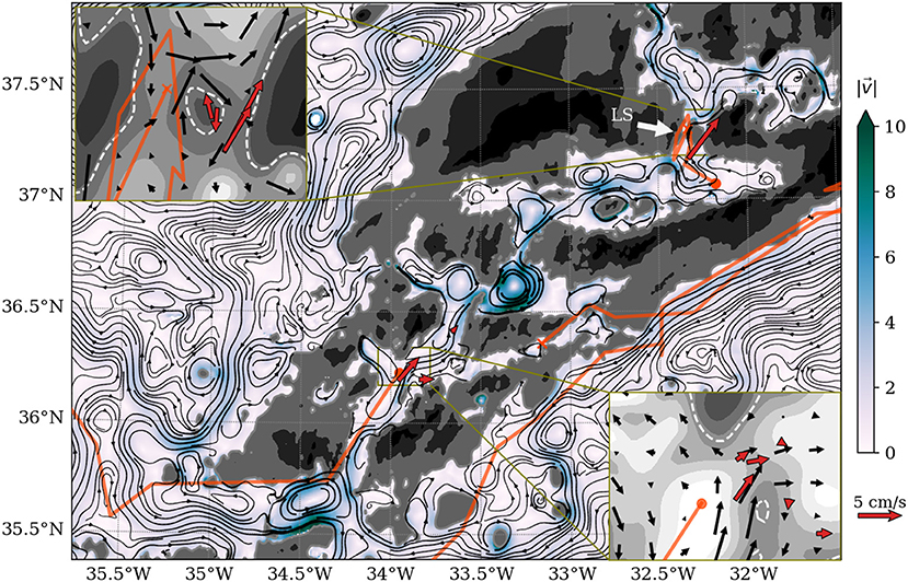
Figure 2. Rift valley circulation at 2,000 m. The mean flow from numerical modeling is shown in black (“streamplot” with the line thickness proportional to the speed amplitude) and colors further indicate its magnitude. Superimposed are two ARGO float tracks near 1,990 m inside the rift valley and two other ones near 1,500 m flowing southward along the eastern flank of the ridge (orange, with the location of the release and last record indicated by a plain circle and a cross, respectively). Red arrows represent the mean velocity from selected moorings near the Rainbow vent field (2,100 m deep) and in the East canyon at Lucky Strike (1,875 m, LS label). Insets show zooms over these regions, representing the mean flow with black arrows. Black shading indicates bathymetry (using the same convention as in Figure 1) and white dashed contours in the insets indicate the depth at which the mean velocity is computed from the simulation (2,100 m at Rainbow, 1,800 m at Lucky-Strike, to match most of the available observations). At Rainbow, all 6 moorings available in the region are plotted. At Lucky-Strike, moorings are taken from (going west to east): Momar (1,700 m), DIVA (1,680 m), and Graviluck (1,930 and 1,874 m).

At most locations, the up-valley current is intensified along the right flank (looking downstream) of the rift valley. It is particularly visible in the AMAR and FAMOUS segments (see also the vertical cross-sections of the mean flow discussed in the next section). A general feature of the rift-valley dynamics is that currents are flowing along the topography in the direction of Kelvin wave propagation. Correspondingly, a weaker return branch flows downward along the opposite flank within the valley (e.g., southward along the west inner flanks), as further described below. This is consistent with the presence of cyclonic gyres within the basins, e.g., near 33.3°W, 36.6°N, with associated velocity of magnitude up to 10 cm/s, size of a few tens of kilometers, and associated value of relative vorticity of order 0.5f. Finally, a mean flow is also observed along the outside flanks of the ridge, again flowing in the direction of Kelvin wave propagation, i.e., in the Northeastward/Southwestward direction along the West/East flank. The direction of the mean flow along the East flank is supported by the trajectory of two distinct ARGO floats (calculated by linearly interpolating consecutive surfacing positions, every 20 days), albeit at shallower depths (1,500 m, IDs: 6900166 and 6900212).

Insets in Figure 2 show the currents zoomed over the Rainbow and Lucky-Strike passages, including additional in-situ data. At Rainbow, water coming from the south and flowing along the right flank (right of the float release point) turns eastward into the sill. A very good agreement is observed between the observations and the numerical simulation at this passage. A fraction of the flow, downstream of the passage, continues veering southward along the slope of the Rainbow ridge. The mean velocity reaches 5 cm/s, but much higher values can occur, as discussed in the next section.

The flow is more complex at the Lucky-Strike passage. Observed velocities suggest a strong northward flow in the East canyon, which is associated with increased dissipation and mixing (St. Laurent and Thurnherr, 2007) and well evidenced by the two current time series around 1,900 m from the Graviluck cruise (2006–2007). Over the volcano, two moorings (Momar, 2015–2016, 1,700 m and DIVA, 1994–1995, 1,680 m), which are less than 2 km apart from each other, show year-mean currents in opposite directions. While this could be associated with different flow patterns at a timescale of a year, it is also compatible with the general pattern of currents flowing along the wall to their right within the canyon. With that in mind, the southward current corresponds to the shallower return branch that flows along the west wall of the east canyon, while the northward current takes place outside of the canyon, being closer to the lavae lake at the center of the volcano. In the numerical model, the topography is too smoothed to properly reproduce the east canyon passage: the maximum depth of the canyon is less than 1,950 m, while it is deeper than 2,000 m in reality. Consequently, the main northward flow between the two basins is largely blocked in the east canyon by the under-resolved topography and is thus deviated to the west canyon, which is visible as a thicker streamline connecting the two basins in the global streamplot (Figure 2). The chaotic behavior of the trajectory of the float deployed in the south Lucky-Strike basin (ID: 4900302) could be consistent again with the up- and down-valley flow structure on the east and west flank of the west canyon, and also with the higher variability of the currents at this location (see discussion in the next section).

Velocity records with similar characteristics—6-week-average velocities directed up-valley with typical amplitude between 3 and 8 cm/s—were collected with current meters moored near the seabed in the FAMOUS segment in the 1970s (Keller et al., 1975), and 2-week long records from a bottom-mounted ADCP deployed in an overflow in the Lucky Strike segment (Thurnherr et al., 2008). This supports that the velocity records shown in Figure 2 can be considered representative for the flow in this section of the rift valley.

3.2.2. Cross-Valley Structure of the Mean Flow

The available velocity data from moored instruments only provide limited information on the lateral (cross-valley) structure of the sub-inertial circulation in the rift valley. However, they can be used collectively and in combination with numerical simulations to build a three-dimensional picture of the mean flow. Vertical sections of the mean current at three passages (sills) are shown in Figure 3. The data shown are 3-month averages from the numerical simulation and mean currents from year-long moorings that are close enough to the section (within 700 m). In the case of the Rainbow and AMAR-FAMOUS passages, the actual location of the sill corresponds to the deepest passage in the left part in the section, while the other one is the intersecting downstream basin.

FIGURE 3

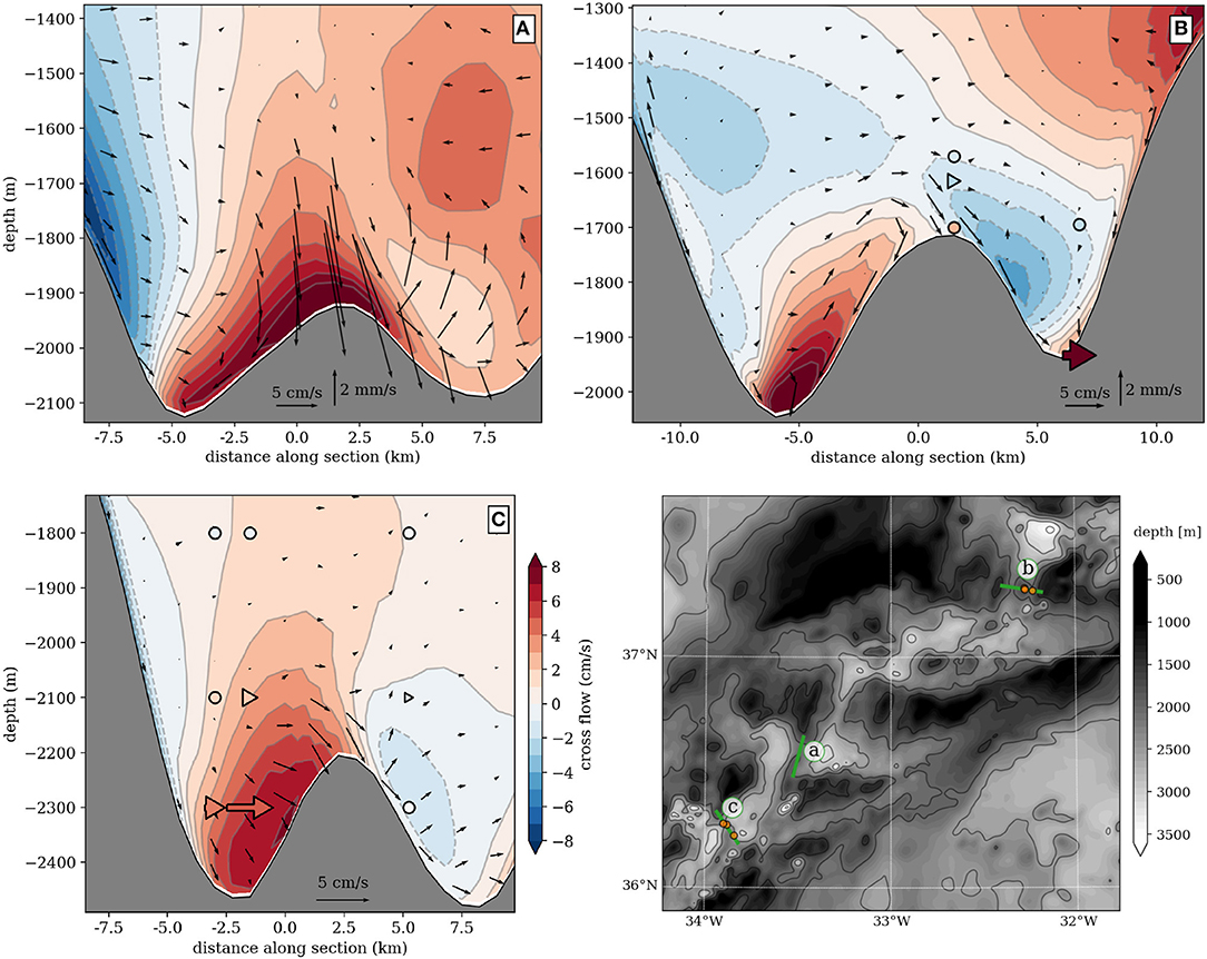
Figure 3. Mean flow at vertical sections across the AMAR-FAMOUS (A), Lucky-Strike (B), and Rainbow (C) passages, over the 700 m above the deepest point. Colors indicate the cross-section velocity, for an observer oriented in the same direction as the dominant up-valley flow, and arrows represent the velocity in the section plane. Note that arrows pointing toward (or away from) the topography result from the combination of the cross-section component of the flow and cross-section gradient of the topography (e.g., at Rainbow, the flow is flowing downward along the downstream flank of the sill). Additional velocity data from observations are superimposed in plain arrows for Rainbow and Lucky-Strike, using the same color-scheme for the cross-section component and the same scale for the along-section component (vertical velocity was not measured). A dot is used if the along-section observed velocity is smaller than 0.4 cm/s. The topography is taken from the numerical simulation. The lower right panel shows the location of the sections (green line) over the topography (shallower depth are darker, following the same convention as in Figure 1), as well as the locations of the in-situ data (orange circles). All observations are within 700 m of the closest point on the sections.

At the Rainbow sill, the agreement between the numerical simulation and the observations is remarkable, as previously noticed in the corresponding inset of Figure 2. The agreement is not so good at the Lucky-Strike passage, most likely because of topographic smoothing as previously discussed. Velocity records from the Graviluck cruises show a very strong current in the East canyon (at a depth which is actually below the seafloor in the smoothed topography used for the simulation). At the scale of the entire passage (containing both canyons), the model reproduces a net up-valley flow below 1,800 m. The corresponding transport is 0.05 Sv (0.06 Sv up-valley, 0.02 Sv down-valley), to be compared with previous estimates from observations of 0.1 Sv (Thurnherr et al., 2008).

At all three passages, the mean flow exhibits a strong up-valley branch with speeds greater than 8 cm/s, bottom intensified on the right flank of the valley, and extending a few hundred meters above with a slight tilt to the right. On the other side of the valley, a thinner return branch is visible, with lower speeds, and partially extending above the up-going branch. The latter feature is clearly visible in the western Lucky-Strike canyon (Figure 3, right panel). At Rainbow, the observations indicate a weak down-valley flow at 1,800 m, which will be further discussed in section 4.1. An analogous record collected on a mooring deployed upstream in the same overflow at Rainbow shows the same pattern, thus supporting that the northeastward deep overflow fills the entire width of the deep rift valley. Estimates of the mean transport across the Rainbow sill below 2,000 m were made by Thurnherr and Richards (2001) and Thurnherr et al. (2002) who found Q = 0.065 and 0.07 Sv, respectively. In our realistic numerical simulation, the integrated transport below 2,000 m is 0.095 Sv.

LADCP velocities from surveys carried out near the Rainbow (Thurnherr and Richards, 2001) and Lucky Strike (Thurnherr et al., 2008) vent fields also contain useful information on the spatial structure of the rift-valley circulation on time scale of a few weeks, although the dominant semi-diurnal tidal variability obscures the sub-inertial patterns in many of the individual profiles. At the two sites there are clear indications of an up-valley deep current and a shallower down-valley current flowing with the (rising) bottom slope on their right. This pattern is particularly clear in the center of the Lucky Strike segment, where the water flowing along the rift valley below 1,600 m must pass through either of the two canyons (Figure 4). During two LADCP surveys carried out 1 year apart, the northeastward (up-valley) currents were stronger in the eastern passage, whereas the southwestward flow was only observed west of the volcano at depths shallower than 1,900 m. At even shallower depths there are indications that a down-valley flow is prevalent in the Lucky Strike segment, as also shown in the numerical simulations (Figure 3, right panel). In particular, 2 year-long current-meter records collected near 1,600 m at the peak of the Lucky Strike volcano, show southward mean currents both in 1994–95 and 2001–02 (Khripounoff et al., 2000, 2008; Thurnherr et al., 2008).

FIGURE 4

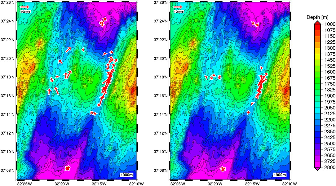
Figure 4. LADCP velocities at 1,900 m observed during two surveys of the Lucky-Strike segment center in 2006 and 2007 (St. Laurent and Thurnherr, 2007; Thurnherr et al., 2008).

Direct evidence for the potential transport induced by the rift-valley circulation is provided by the trajectories of a neutrally buoyant Argo float (ID: 5902322) deployed in the rift valley in 2007 and programmed to drift around 1,990 m (±15 m). The float was released near the Rainbow overflow and drifted along the rift valley for about a month before leaving the MAR crest through a channel north of the Oceanographer fracture zone (Figure 2). The first two 20-day displacements of the float are consistent with strong down-valley flow with mean straight-line speeds of 3.5 and 5 cm/s, respectively, and the surfacing positions strongly suggest advection along the northwestern rift-valley wall.

3.3. Rift Valley Hydrography

We now describe the stratification and density distribution in the rift valley, in connection with the topography and the mean currents.

3.3.1. Region-Scale Hydrography

Since the deep rift valley is topographically separated from the ridge flanks below 2,000 m, water renewal is driven by inflows across the sills on the valley walls (Fehn et al., 1977; Saunders and Francis, 1985). The inflow from the eastern ridge flank (Thurnherr et al., 2002) already identified in Figure 1 is recognizable in Figure 2 near 34.2°W, 35.6°N. From the numerical simulation, it is difficult to tell whether additional water could come from the West ridge flank through the stream flowing along the fracture zone north of the Oceanographer fracture zone, and adjacent to a cyclonic gyre located at 34.4°W, 35.7°N, or whether these currents mostly consist of recirculating water. The topography suggests that the flow is largely blocked west of this gyre, near 34.65°W, which agrees with previous estimates that this branch is weak compared to the main inflow from the East (Thurnherr et al., 2002). Further North, other possible inflows can be inferred near 34°W, 36.7°N and up in the western corner of the North Lucky-Strike basin, near 32.5°W, 37.9°N. Only the latter passage has been identified from hydrographic evidences and reported in the literature (Fehn et al., 1977; Saunders and Francis, 1985; Thurnherr et al., 2008). The available data suggest however that this northern water does not flow southward along the rift valley but, rather, upwells locally within the deep basin north of the Lucky Strike segment center (Thurnherr et al., 2008).

The properties of the deep rift-valley water are therefore largely determined by the properties of a thin layer of inflowing water. Likewise, the presence of sills and overflows in the rift valley is associated with density selection: each basin receives water with a narrow range of T/S properties from the upstream basin. In the region studied here, the main known source for rift valley water below 2,000 m is an about 200 to 300-m-thick inflow across the eastern rift-valley wall near 35.5°N (see Figures 1, 2; Thurnherr et al., 2002). As the thin layer of inflowing water fills the entire rift valley below the inflow depth, the vertical property gradients, including density stratification, are significantly reduced everywhere in the valley, compared to the corresponding gradients in the ridge-flank water (Fehn et al., 1977; Saunders and Francis, 1985, and see Figure 6 discussed below). The narrow temperature and salinity ranges at the inflow furthermore cause the entire rift valley to have tight T/S characteristics, which facilitates detection of hydrographic anomalies, including those due to lateral exchanges with ridge-flank waters at shallower depths where the valley walls are permeable (Wilson et al., 1995) as well as due to hydrothermal sources and geothermal heating (Thurnherr and Richards, 2001; Thurnherr et al., 2002). Apart from these two types of hydrographic “anomalies,” the T/S properties of the rift valley in our study region are well-described by a linear relationship with an approximately constant stability ratio R_ρ = α∂_zθ/(β∂_zS) ≈ 2.3 (with θ the potential temperature, S the practical salinity, α = 1.47 × 10⁻⁴ °C⁻¹ and β = 7.53 × 10⁻⁴ psu⁻¹) (Thurnherr et al., 2002).

A consistent northeastward along-valley density gradient is visible in the observations and in the model. Segment-scale surveys of the rift-valley hydrography in our study region were carried out in 1992 (FAZAR project), in 1994 (HEAT project), and in 1998 (FLAME project). Inspection of the individual data sets (Figure 5) reveals a consistent northeastward decrease in the temperature and density [the linearity of the T/S properties in the rift valley implies that temperature can be used as an (inverse) proxy for density] of the rift-valley water in each case. (For a detailed discussion of the segment scale hydrographic gradients observed in 1998 see Thurnherr et al., 2002). Since the rift-valley profiles show mutually consistent temperatures and along-valley temperature gradients in the 3 years (left figure panel) we conclude that the data indicate a quasi steady state on time scale of years, at least.

FIGURE 5

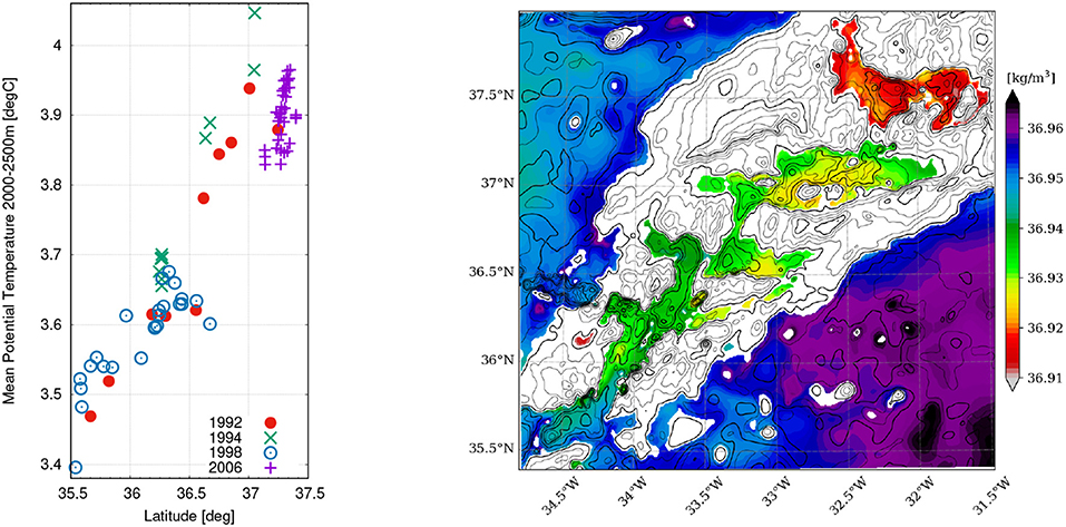
Figure 5. (Left) Vertically averaged potential temperature in the rift valley between 2,000 and 2,500 m from four segment-scale surveys carried out in 1992, 1994, 1998, and 2006; only profiles extending below 2,300 m are shown. (Right) Mean potential density at 2,100 m from the numerical simulation. Topography contours (from the numerical model) are shown in black every 250 m (with a thick contour at 2,000 m).

These hydrographic properties evidenced from multiple surveys are also clearly visible in the numerical simulation (Figure 5, right panel). In particular, water masses at 2,100 m depth are lighter inside the rift valley compared to outside (the mean difference is about 20 g/m²), and potential density exhibits an along-valley gradient with water getting lighter northward.

3.3.2. Evidence of Blockage and Mixing at Sills

The topographic sills impedes exchange of water properties between the basins not only directly by topographic blocking, but also indirectly by causing hydraulic overflows that act as one-way valves for the deep valley water, as previously reported at Rainbow (Thurnherr and Richards, 2001) and Lucky-Strike (Thurnherr et al., 2008). As a result, the dominant horizontal patterns of the deep water temperatures and densities in the rift valley commonly mirror the basin/sill topographic structure, with the horizontal gradients concentrated across narrow sills (Fehn et al., 1977; Thurnherr and Richards, 2001). Indeed, both the observations reported here and the numerical simulations reveal the presence of steps in the density distribution (Figure 5). In particular, the main density drops are associated with the overflow across the sills between the AMAR and the FAMOUS segments, north of 36.5°N. In the numerical simulations, density steps appear more clearly at the Lucky-Strike passage in the northern part of the domain, and to a lesser degree at the passage between the AMAR and FAMOUS segments.

Figure 6 shows density profiles across the three prominent sills of the region. All profiles are characterized by a reduction in density stratification below ≈2,000 m, i.e., in the topographically isolated rift valley water. At each sill the density of the deep rift-valley water on the upstream side of the sill (with respect to the deep mean northeastward along-valley current; see below) is higher than the corresponding density on the downstream side. The density drop extends 100–400 m above the sill depth, and in each case a layer of reverse gradients is visible above. Assuming flat isopycnals higher in the water column, the cross-sill density gradients imply corresponding pressure gradients that force water across the sills. Comparison of the individual panels of Figure 6 supports the continuous north-eastward density decrease in the rift valley water.

FIGURE 6

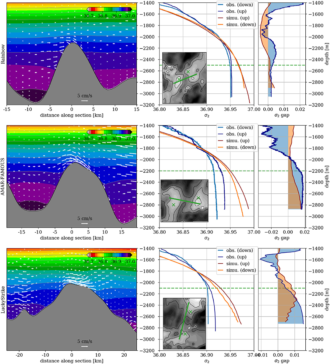
Figure 6. Density changes across three prominent sills in the rift valley, namely the Rainbow sill near 36.25°N (upper row), the AMAR-FAMOUS overflow sill near 33.5°W, 36.5°N (middle row), and the Lucky-Strike segment center near 37.25°N (lower row). Left panels show mean potential density anomaly referenced at 2,000 m at vertical sections across the sill, together with the along-section component of the mean flow in white arrows. Location of the sections are indicated by green lines on the mapped bathymetry (gray) shown in the middle panels. Middle column: upstream (darker) and downstream (lighter) potential density vertical profiles from CTD stations (blue shade) and from the numerical simulation (red shade—3-month average). Right column: upstream—downstream potential density difference. The location of the profiles are indicated by green crosses in the inset maps of the middle panels. The dashed green horizontal line indicates the maximum depth of the sill. CTD profiles at the AMAR-FAMOUS passage are taken in 2007 (MOMARdream cruise) and are very similar to equivalent profiles in 1997 (Thurnherr and Richards, 2001, Figure 7A).

In the numerical simulation, the upstream-downstream density difference is qualitatively reproduced, although the stratification is larger compared to the observations over the full range of depths shown. Numerical ocean models have a perennial problem of misrepresenting the water mass properties, and in particular the salinity. This is caused, among other things, by the fact that the initial state from the parent simulation is imperfect (in our case, SODA is known to overestimate salinity in some regions). Furthermore, the model is missing some sources of mixing due to the missing geothermal heating, and partially underresolved processes at high-frequency (see subsection 4.1 for a description of the currents variability). The T/S/ρ properties must be compared keeping in mind these biases, therefore we will only comment qualitative comparisons and favoring spatial gradients. The exact locations of the upstream and downstream profiles are important because horizontal gradients of density are also present within the basins at each edge of the passage due to the basin-scale circulation (through thermal-wind relationship), especially in the FAMOUS basin. Ideally, density differences should be evaluated along streamlines, which is not practicable (streamlines are not constant). We chose to use the location of the observations for the vertical profiles of density in the simulations, while the sections are approximately tangent to the flow at the center of the sills.

At two sills, out of the three shown in the figure, direct velocity observations confirm the presence of hydraulically controlled overflows (Thurnherr and Richards, 2001; Thurnherr et al., 2008), which is largely consistent with the structure of the mean along-section flow from the numerical simulation observed at all three passages (Figure 6, left column). There is a vast literature on hydraulic control at overflows in the ocean, from theoretical studies—mostly using reduced-gravity layered models (e.g., Whitehead, 1998; Nielsen et al., 2004)—to in-situ observations (Pratt et al., 2000; Clément et al., 2017). It shows that such overflows are associated with enhanced mixing, in particular when the flow becomes supercritical (with respect to the local Froude number) and gives rise to a hydraulic jump downstream of the sill. This provides another mechanism for the observed reduction in stratification within the rift valley, in addition to the density selection mentioned above. Mixing associated with supercritical overflows at Rainbow and Lucky-Strike has indeed been evidenced by several observational studies (Thurnherr et al., 2002; St. Laurent and Thurnherr, 2007; Tippenhauer et al., 2015). The dipolar structure of the upstream-downstream density difference is a signature of such overflow-induced mixing (Thurnherr et al., 2005).

A possible explanation for the numerical simulation showing reduced density gap and greater stratification within the rift valley could be a lack of mixing, e.g., at the overflows. Investigation of the structure of the overflow at Rainbow along the same vertical section as shown in Figure 6 (upper row) in the numerical simulation indeed reveals that events of strong current at the passage are associated with higher values of vertical diffusivity in the model, of the order 5 × 10⁻² m²/s (the background value used in the simulation is 10⁻⁵ m²/s). However, the region of enhanced vertical shear and diffusivity extends only over a few grid points (less than 10, both in the vertical and the along-stream directions), henceforth the dynamics is certainly not accurately resolved and more quantitative investigation is left for future work.

The dependence of the upstream-downstream density difference with the location is however in qualitative agreement between the simulation and the observations: for instance, it is clearly smaller at Rainbow compared to the other two passages. Repeated samplings at the Rainbow sill and Lucky Strike indicate that the situation is more complex than the above discussion suggests. In particular, out of four distinct profiles across Rainbow Sill, only two look like the figure while the other two show a much smaller density drop across the sill—thus mitigating the apparent discrepancy between observations and numerical simulations at this passage. We checked in the simulations that, considering two points relatively close (around 5 km) and approximately lying over the same streamline on each side of the sill, the density difference and the current indeed exhibit temporal variations (not shown). Both quantities are correlated and the time average is consistent with the vertical dipole depicted above and inferred from the observations. The three repeated profiles at Lucky Strike also show significant variability in the vertical structure of the cross-sill density differences.

4. Variability and Forcing

4.1. Temporal Variability

We previously described the spatial structure of the mean flow, using long-time in-situ records and numerical simulation. The dynamics in the rift valley exhibits significant temporal variability, as already discernible from Figure 4, which shows differences in the horizontal patterns of the current at two different times. The time variability is investigated here based on 2 year-long time series recorded in 1997–1998 at Rainbow (FLAME D) and in the AMAR region (FLAME F), at three different depths. The two locations were previously shown to have very different dynamics (Thurnherr et al., 2002). Figure 7 shows Horizontal Kinetic Energy (HKE) spectra and Kernel Density Estimate¹ (KDE) of the current from the in-situ data (blue lines), in comparison with similar quantities computed from the numerical simulation (red lines).

FIGURE 7

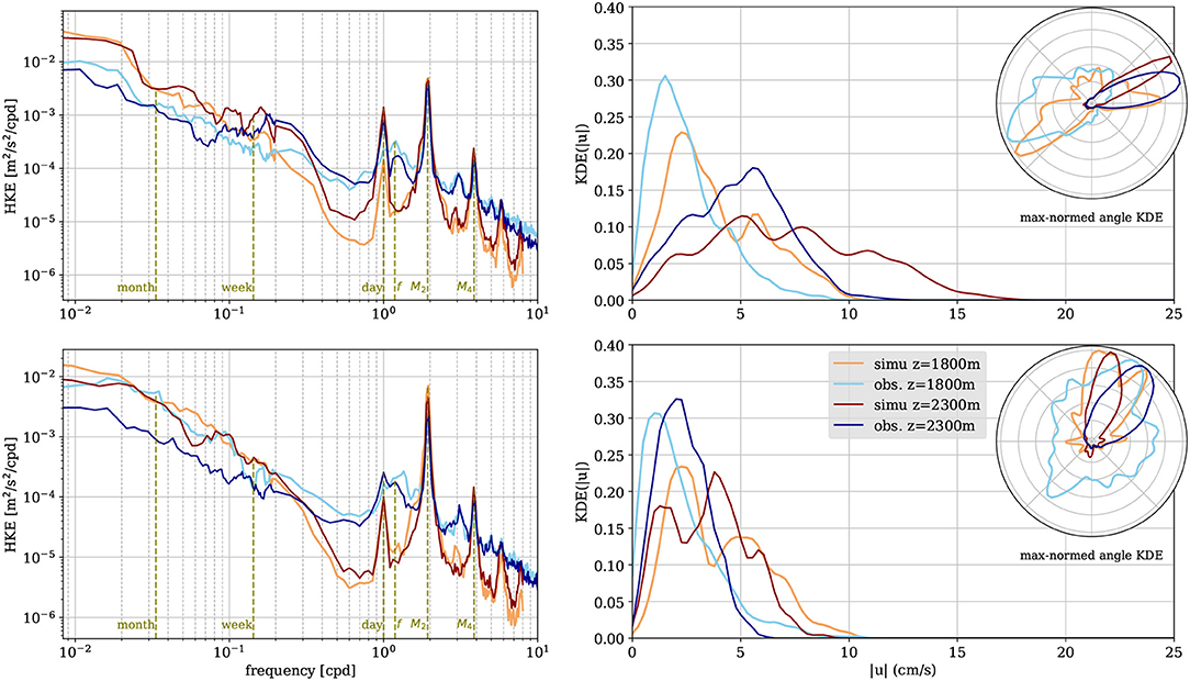
Figure 7. Left column: Horizontal Kinetic Energy Power Spectral Density, and right column: Kernel Density Estimates of low-pass filtered velocity magnitude and angle (polar-coordinate insets, normalized by the max value of the distribution to improve readability), in the Rainbow overflow (upper row) and downstream in the AMAR segment (lower row), from the numerical simulations (red/orange colors) and in-situ observations (blue).

The HKE spectra show very similar variability at the different depths (Figure 7, left panels). Peaks appear at diurnal and semi-diurnal frequencies and at their harmonics, with a good agreement between the observations and the simulation. The numerical model lacks energy in the near-inertial band (≈ 0.5–2 cpd) by almost an order of magnitude, except at the diurnal frequency. A probable reason is the daily wind forcing, used for imposing the wind stress at the surface of the simulation, which does not inject enough near-inertial wave energy. Another possibility is that the resolution is too coarse for the model to fully capture near-inertial currents and oscillations generated through current-topography interactions. The model also lacks energy in between the tidal harmonic peaks (M₂, M₄, …), which may reflect an imperfect resolution of wave-wave interaction mechanisms, and/or the lack of energy in the near-inertial band resulting in weaker harmonics generated through wave-wave interaction (van Haren, 2016).

The energy content at sub-inertial frequencies is of particular interest for the deep currents that are discussed in this paper. HKE spectra show that significant variability is present below f, in particular at a time scale of about 1 week at Rainbow, meaning that the deep rift-valley currents are turbulent. Kernel Density Estimates (KDE) of the low-pass time filtered time series (using an order 4 Butterworth filter with frequency cutoff 1/30 h⁻¹, thus filtering out mostly wave-related motions) are given in Figure 7. The most glaring differences—the magnitude and direction in particular of the deep currents—appear consistent with the distinct dynamical settings, as well as with topographic steering effects at the two sites. At both locations, the current at 2,300 m is mostly unidirectional, directed northeastward (up-valley flow), with typical magnitude of around 5 cm/s at Rainbow and 2.5 cm/s at AMAR. Out of the 372 daily averaged records (not shown), only 3% show reversal of the along-valley flow at Rainbow, while this value increases to 15% at AMAR. The current is mostly in the same direction at 2,100 m (not shown), although much weaker in magnitude and more spread in the angular distribution. Correspondingly, the fraction of days with flow reversals is significantly higher at 27%. At 1,800 m depth, the counter-flow is clearly visible at Rainbow with typical values of 2 cm/s. Hence, during the year-long sampling, the overflow near the Rainbow vent field acted as a one-way valve for the along-valley flow below 2,000 m. At 1,800 m, which is above the layer of weakly stratified valley water (Figure 6), the current-meter records from the overflow show long (several days up to more than a month) pulses of strong (≈ 5 cm/s) down-valley currents, and these pulses dominate the yearly average. The downstream (AMAR) record at 1, 800 m is qualitatively more different from the one in the overflow, as there were no strong down-valley pulses recorded and, as a result, a weaker mean current. The angular KDE is indeed more isotropic for the in-situ record, whereas a net up-valley flow is still visible in the simulation.

The currents in the rift valley can be discussed in terms of two major dynamical components: the internal tides and the low-frequency current. We investigate more carefully the characteristics of each kind of motion by repeating the previous diagnostics for different frequency bands, and computing the HKE spectra from the different numerical simulations with different forcings (with tides, without tides, and tide-only without nesting nor surface forcings). The results are shown in Figure 8 (left panel) using data in the East Lucky-Strike canyon (in-situ record from Graviluck survey). The simulation without tidal forcing has less variability at timescales shorter than a few days. Including tidal forcing thus adds variability not only in the super-inertial frequency range, but although in the near- and sub-inertial range, which confirms the importance of internal tides for the ocean energetic and the accuracy of ocean numerical models (e.g., Arbic et al., 2012). Conversely, the tide-only simulation exhibits tidal peaks magnitude similar to the simulation with full forcing, but lacks energy in-between the peaks—which supports the fact that a significant fraction of the wave continuum requires energy in the near-inertial band or interaction with the vortical turbulence (in a broad sense, i.e., motions already present in the no-tide simulation). Moreover, low energy values on each side of the diurnal peak indicates that variability at these frequencies results from non-linear interactions between internal tides and balanced turbulence.

FIGURE 8

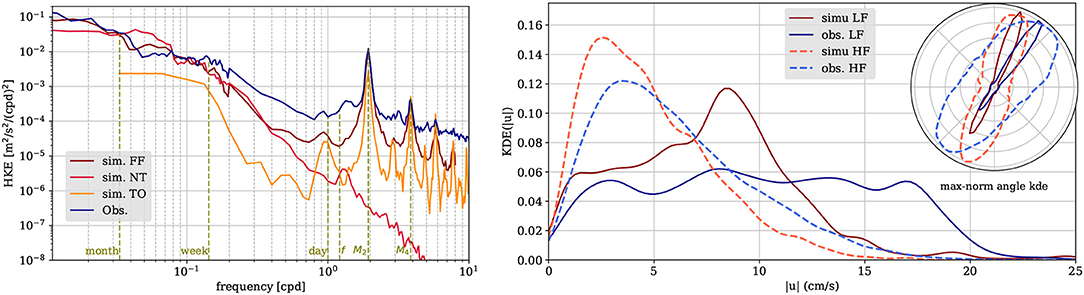
Figure 8. Kinetic Energy spectra (left) and Kernel Density Estimates (right) at a mooring from Graviluck experiment (M1, 1,870 m). The different curves in red to orange shades correspond to different numerical simulations (FF, Full Forcing; NT, No Tidal forcing; TO, Tidal forcing Only). In the right panel, Kernel density estimates are computed on low-pass and high-pass filtered time series (“LF” and “HF,” respectively).

In the right panel of Figure 8, Kernel Density Estimates of low-pass and high-pass time-filtered data (with cutoff frequencies of 1/30 h⁻¹ and f, resp.) are presented. The low-frequency component shows the same unidirectional current as mentioned previously at Rainbow and AMAR. However, the angular distribution extends toward the opposite direction (with fewer occurrences: about 10% of the values are in the down-valley direction), which is indicative of flow reversals in the canyon. Because of the downgraded local topography in the simulation and the resulting lack in up-valley currents in the East Lucky-Strike canyon, the corresponding speed is smaller (reaching ≈10 cm/s) compared to the observations, which has typical values reaching ≈17 cm/s. Likewise, the angle shift between the numerical simulation and the observations reflects the different topography. The high-frequency component is dominated by the tides: the angular distributions show ellipses, aligned along the same axis as the low-frequency component, thus reflecting the strong topographic constraint. The distributions in current amplitude are very different between the high-frequency and the low-frequency components. The former is narrower with a peak at ≈4 cm/s and decreases at higher values, reflecting the regularity of the tidal flow. On the contrary, the distribution of the low-frequency flow is nearly flat over a wide range of values, thus associated with a high variance and relatively high occurrence of intense currents.

4.2. Dynamical Origin and Forcing

Upwelling currents within narrow canyons can be forced by the density gradient resulting from bottom-enhanced mixing over the sloping topography (e.g., St. Laurent et al., 2001; Thurnherr et al., 2005; Clément and Thurnherr, 2018), which is often predominantly generated by internal tides. Because of topographic blocking, the cross-slope component of the Ekman-like response is suppressed, and the resulting flow is mostly an along-canyon overturning cell with the density field in advective-diffusive balance. The Earth rotation affects the dynamics of the along-valley flow which gets deflected along the topographic slope to its right, especially in larger valleys with typical width of a few internal deformation radii. This mechanism, however, ignores the potential impact of (sub-)mesoscale turbulence and associated pressure and velocity perturbations. Given this complex configuration, it is very challenging to attribute the dynamical origin of the deep currents and of their variability. While density gradients induced by differential mixing is likely an important mechanism at play, the role of mesoscale eddies, e.g., in transferring momentum to the mean field (Holloway and Wang, 2009; Venaille et al., 2011) could be important as well.

To get some insight on the relative importance of these different dynamical factors, we compare the deep-ocean currents between the three different numerical configurations introduced previously: tide-only, no-tide, and full-forcing. This comparison allows to investigate the impact of each dynamical component—namely the tides and the mesoscale turbulence—on the low-frequency deep currents, neglecting their interaction. Some aspects of the corresponding dynamics were already discussed in the previous subsection (see Figure 8, left panel and corresponding discussion), and it was shown that the tide-only simulation is much less energetic in the sub-inertial frequency range. However, it does have a low-frequency circulation emerging from the initial rest state. Figure 9 shows the horizontal structure of the mean flow obtained in the different runs at 2,000 m depth, as well as the vertical structure at a section located near the center of the FAMOUS sector, around 36.8°N [this passage corresponds to the first observations of deep currents and associated density gradients reported in the region by Keller et al. (1975) and Fehn et al. (1977)]. The time average is computed over four months for the realistic runs with and without tides and 2 weeks (starting at 1 month) for the tide-only simulation.

FIGURE 9

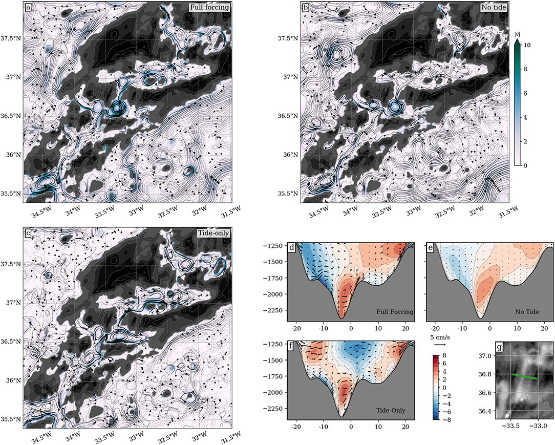
Figure 9. Comparison of different simulations with different forcing, as seen from the mean horizontal current at 2,000 m (a–c—same convention as in Figure 2) and the vertical structure across a section in the Famous segment (d–f, and localization of the section in g—same convention as in Figure 3). The different configurations correspond to full forcing (a,d), no tide (b,e), and tide-only (c,f).

As expected, none of the simulations with partial forcings reproduces the structure of the flow as observed in the fully-forced simulation. However, it appears that some portions of the current are adequately reproduced independently in these truncated configurations. For instance, the circulation in the fracture zone between the AMAR and the FAMOUS segments (around 36.6°N) does have a cyclonic gyre in the simulation with no tidal forcing. The circulation in the FAMOUS passage, near 36.7°N, produced by the tide-only simulation shows some similarities with the reference run as well. This is particularly visible in the vertical section at 36.8°N, which shows that the tide-only simulation produces an up-valley flow with a magnitude comparable to the reference run, as well as a thin counter flow on the west flank of the passage, between 2,000 and 1,800 m. Interestingly, for this particular example, the currents observed in the simulation with no tide are weaker, although sharing some similarities. It also appears that the flow close to isolated seamounts (e.g., in the southern part of the domain shown, between 33.5° and 32°W, or near the ridge flank, following the 2,000 m isobath on the East side) is largely forced by the tides, possibly through adjustment to the bottom-enhanced mixing or tidal rectification. To summarize, both simulations with incomplete forcing exhibit a low-frequency circulation at depth, with a magnitude comparable (although weaker) to the reference run, thus showing that both dynamical components present in each run—the tides and the mesoscale turbulence—play a role of comparable importance in generating this deep flow.

We now give a more quantitative analysis based on the horizontal kinetic energy in the rift valley (north of 35.7°N) at 2,000 m. Figure 10 shows the spatial average of the HKE spectra computed over a period of 8 months as well as the time series (over 2 months) and the probability distribution of the horizontally averaged HKE of the low-frequency currents, thus extending the previous results (Figures 7, 8) to the entire rift valley. Both runs with nested turbulence exhibit similar properties: the HKE spectra follow a −2 slope (slightly shallower, albeit steeper than −5/3) in the range of timescales between 1 month and a few days and are flatter at lower frequencies. There is significant variability at super- and near-inertial frequencies, although the numerical simulations underestimate the variability in the latter frequency range compared to the observations. One must keep in mind that the observational data are sparsely distributed in space and do not cover the entire rift valley. The variability is dominated by the tides at high frequency.

FIGURE 10

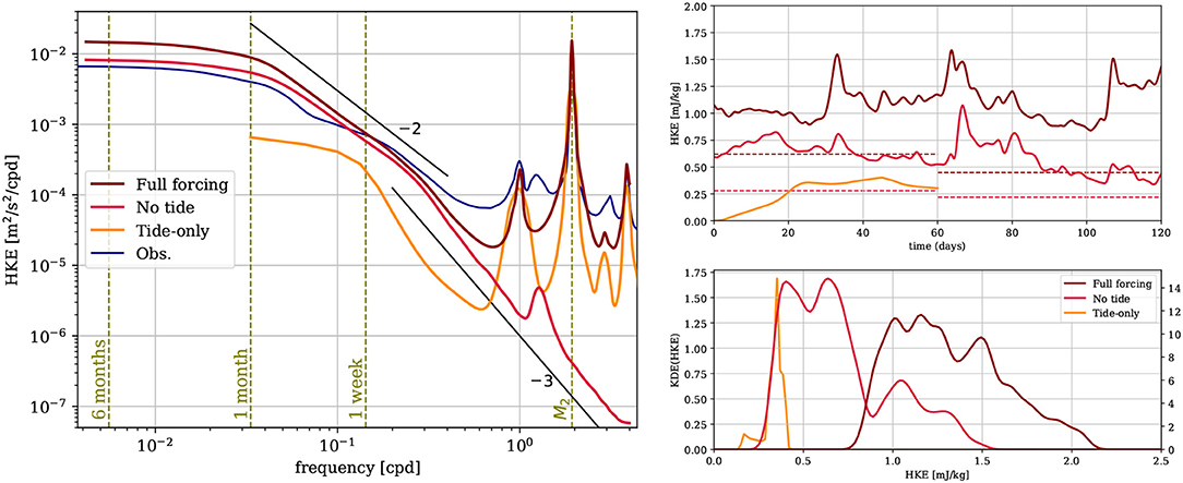
Figure 10. Left panel: Horizontal Kinetic Energy spectra at 2,000 m, spatially averaged in the rift valley above 35.7°N for the different numerical runs. For the tide-only simulation, the spectra are computed over 1 month between day 25 and 55. The spectrum in blue is taken from averaging data from different current meters between 1,800 and 2,100 m on the moorings at Rainbow and Lucky-Strike. Note that energetic eddies present in the basins cannot be measured by these moorings because of their position, which probably explains smaller energy density at low frequencies (< 1 day⁻¹). Right panel, top: Evolution of the Horizontal Kinetic Energy of the low-pass filtered velocity (cutoff frequency 1/48 h⁻¹) over four months (only 2 months are available for the tide-only run), spatially averaged in the rift valley. Dashed lines indicate HKE of 2-month averaged velocities. Right panel, bottom: KDE of the distribution of the low-frequency HKE shown above, computed over the same period as the spectra in the left panel.

In the subinertial range, the two realistic runs exhibit significant variability, with relative variations of the low-frequency HKE at 2,000 m (with 2-days cutoff period) of about 50% (Figure 10, right panels). Correspondingly, the low-frequency HKE has a broad distribution (with different means for each simulation, as discussed below). A noticeable feature in the time series of the spatially averaged low-frequency HKE is the presence of sudden rises, usually followed by slower decreases, which reflects rapid intensification of the currents taking place over large portions of the valley. Since this variability is observed with or without tidal forcing and manifests itself at the scale of the entire rift-valley, we can infer that it is driven by the overlying mesoscale turbulence.

In the tide-only simulation, the spatially-averaged HKE of the low-pass filtered velocities reaches 0.35 mJ/kg at the spring tide that occurs 22 days after the simulation began, then slightly decreases to 0.34 mJ/kg at the subsequent neap tide and then slowly increases to reach 0.4 mJ/kg at day 45. After this period, the tidal forcing is switched off and the low-frequency mean energy slowly decreases down to 0.3 mJ/kg at the end of the simulation (60 days). Thus, the tide-only simulation has not converged to a steady regime as far as the kinetic energy content is concerned. We may however expect that the adjusted circulation would not reach significantly higher values considering the small decrease observed around day 30. The steadiness of this time evolution as well as the power spectra density estimate (Figure 10, left panel) show that the tide-only simulation has significantly less variability compared to the realistic runs, while the mean currents have nearly the same magnitude as the no-tide run, as evidenced by the dashed lines in Figure 10 (top right panel) showing the HKE of the 2-month averaged currents, and the probability distribution (Figure 10, bottom right panel). This supports the previous hypothesis that the rift-valley current variability is predominantly forced remotely, likely by the mesoscale turbulence, rather than of intrinsic nature.

Although the tides do not seem to be directly associated with great sub-inertial variability, they do have an impact on the low-frequency currents. In the range of timescales between a month and a few days, the fully-forced simulation is about 1.4 times more energetic (taking the ratio of the spectral HKE density) than the no-tide run. The same ratio goes up to 1.8 at longer timescales, where the spectra are much shallower. This difference, and the fact that it increases with decreasing frequency, is ascribable to the contribution of the internal tide, which thus does not generate variability in itself (the corresponding spectrum is almost an order of magnitude lower than the realistic runs) but provides energy to the mean flow. Indeed, the HKE for the currents averaged over the 4-month period shown in Figure 10 is 0.43 mJ/kg in the full-forced simulation, while it is 0.2 mJ/kg in the simulation with no tidal forcing, and the 2-week average in the tide-only simulation gives 0.32 mJ/kg (the average is taken from day 30 to 45 in this simulation). This is supported by the probability distribution of the low-frequency current HKE (Figure 10, bottom right panel) for each simulation: the distribution of the fully-forced run is very similar to the no-tide run, shifted toward greater values by about the mean value of the very narrow distribution of the tide-only run.

From the previous results, we conclude that most of the variability at timescales from a few days to a month within the rift valley is dominated by the overlying eddy turbulence. On the other hand, the very low frequency component of the mean flow (at timescales longer than a month) is significantly impacted by the internal tides. Thus, tidal and mesoscale dynamics are both important in forcing the deep circulation in the rift valley. Further work should focus on the details of the forcing and investigate the role of the different possible mechanisms: density gradient generated through mixing on the one hand, and direct momentum deposit through (tidal) rectification mechanism or eddy-topography interactions on the other hand.

5. Discussion and Conclusion

Abyssal flows at mid-ocean ridges strongly interact with the seafloor, resulting in complex patterns that influence the dynamics of deep-sea ecosystems. In particular, the habitats of hydrothermal vents are sensitive to the state of the deep ocean, which is thus critical to their dynamics, their connectivity, and their vulnerability. This is also a major issue in the context of deep-sea mining and exploitation.

During the last decades, several surveys carried in the rift valley of the North Mid-Atlantic Ridge (MAR) between 35°N and 38°N have provided independent indications of an up-valley mean flow around 2,000 m and deeper, associated with a continuous up-valley diminution of the potential density. Besides having an impact on the transport of biogeochemical species and the hydrothermal plumes, this flow is associated with net upwelling of dense waters within the valley. Both effects are relevant in many regions of the deep ocean (over mid-ocean ridges), thus impelling the need of having a better understanding of the rift valley circulation. For this purpose, we used high-resolution realistic numerical simulations of the flow in the region, combined with different in-situ observations, to investigate the dynamics and the hydrography in the rift valley.

Our results confirm the presence of consistent up-valley currents and an associated density gradient in the rift valley, unveiling their time-space structure at the regional scale. We showed that these currents form, on average, a continuous flow from the main entrance passage (with most water coming from the eastern flank of the MAR) near 35°N up to the deep basin north of Lucky-Strike (at almost 38°N). The structure of these currents is intensified along the right inner flank of the rift valley (looking downstream), and is associated with a weaker return branch intensified on the left inner wall, and partially overlying the up-valley current.

This deep circulation is fed by internal tides and mesoscale turbulence, which are known to generate horizontal density gradients through vertical and horizontal mixing intensified near the bottom. Whether direct deposit of momentum by these two types of motions plays a significant role remains to be determined. Using different numerical simulations, with different forcing/dynamics included, we showed that mesoscale activity is responsible for most of the subinertial variability of the current. On the other hand, tidal forcing alone is able to generate a mean current with a magnitude comparable to the mean current generated in realistic simulations. Interestingly, tidal forcing also significantly increases temporal variability in the near-inertial band (i.e., at time scales of a few days) and at even longer time scales (down to a few month, by a factor 2). The interaction of the mean currents with the topography within the valley is responsible for spatial variability manifesting itself as meanders and trapped vortices. Temporal variability is also significant at time scales down to a few days, as well as in the super-inertial frequency band: the currents in the rift valley are thus turbulent, with velocity locally greater than 10 cm/s and local Rossby number of the order of 0.5. The presence of sills separating the deeper basins gives rise to hydraulically controlled flows with increased speeds and jumps in density, which are associated with enhanced diapycnal mixing. The accumulated jumps account for most of the rift-valley scale gradient.

The results presented in this paper show that realistic modeling is a valuable tool for investigating the deep-ocean dynamics. The numerical model captures well the deep circulation, provided the local bathymetry used in the simulation is accurate, and emphasizes the interplay of turbulence, internal tides and current-topography interactions. In particular, it allowed us to shed light over the dynamical properties and forcing of the rift-valley currents. However, higher numerical resolution is needed to have a more accurate topography in the model and better resolved dynamics, e.g., at overflows. Further work should investigate more closely some of the dynamical properties of the deep currents, such as the mechanisms involved in the forcing of the flow and the transport induced by the currents. The hydraulic control at sill overflows, as well as their variability and induced mixing, need also being addressed in the context of deep water transformation in similar regions of the ocean.

Data Availability Statement

The datasets generated for this study are available on request to the corresponding author.

Author Contributions

NL diagnosed the numerical simulations, processed some of the in-situ data, prepared most of the figures, and wrote the bulk of the manuscript. JG and GRo ran the numerical simulations. AT provided and processed most of the in-situ data. GRe and PB-A provided the data from Graviluck cruise. All co-authors participated to the scientific reflection and the writing of the manuscript.

Funding

This study was funded by Conseil Général du Finistère, Région Bretagne and ANR project LuckyScales (ANR-14- CE02-0008). NL was supported by the People Programme (Marie Curie Actions) of the European Union's Seventh Framework Programme (FP7/2007–2013) under REA grant agreement PCOFUND-GA-2013-609102, through the PRESTIGE program coordinated by Campus France. Simulations using CROCO were performed using HPC resources from GENCI-TGCC (Grant 2019–A0010107638).

Conflict of Interest

The authors declare that the research was conducted in the absence of any commercial or financial relationships that could be construed as a potential conflict of interest.

Footnotes

1. ^Gaussian kernel density estimate is used here instead of standard histograms to provide a smoother visualization of the occurrence distribution among values.

References

Arbic, B., Richman, J., Shriver, J., Timko, P., Metzger, E., and Wallcraft, A. (2012). Global modeling of internal tides: within an eddying ocean general circulation model. Oceanography 25, 20–29. doi: 10.5670/oceanog.2012.38

CrossRef Full Text | Google Scholar

Baker, E. T., and German, C. R. (2004). On the global distribution of hydrothermal vent fields. Geophys. Monogr. Ser. 148, 245–266. doi: 10.1029/148GM10

CrossRef Full Text | Google Scholar

Beaulieu, S., and Szafranski, K. (2018). Interridge Global Database of Active Submarine Hydrothermal Vent Fields, version 3.4. World Wide Web electronic Publication. Available online at: https://vents-data.interridge.org.

Google Scholar

Becker, J. J., Sandwell, D. T., Smith, W. H. F., Braud, J., Binder, B., Depner, J., et al. (2009). Global Bathymetry and elevation data at 30 Arc seconds resolution: SRTM30_PLUS. Mar. Geod. 32, 355–371. doi: 10.1080/01490410903297766

CrossRef Full Text | Google Scholar

Carton, J. A., and Giese, B. S. (2008). A reanalysis of ocean climate using simple ocean data assimilation (SODA). Mon. Weather Rev. 136, 2999–3017. doi: 10.1175/2007MWR1978.1

CrossRef Full Text | Google Scholar

Clément, L., and Thurnherr, A. M. (2018). Abyssal upwelling in mid-ocean ridge fracture zones. Geophys. Res. Lett. 45, 2424–2432. doi: 10.1002/2017GL075872

CrossRef Full Text | Google Scholar

Clément, L., Thurnherr, A. M., and St. Laurent, L. C. (2017). Turbulent mixing in a deep fracture zone on the Mid-Atlantic Ridge. J. Phys. Oceanogr. 47, 1873–1896. doi: 10.1175/JPO-D-16-0264.1

CrossRef Full Text | Google Scholar

Conway, T. M., and John, S. G. (2014). Quantification of dissolved iron sources to the North Atlantic Ocean. Nature 511, 212–215. doi: 10.1038/nature13482

PubMed Abstract | CrossRef Full Text | Google Scholar

Egbert, G. D., and Erofeeva, S. Y. (2002). Efficient inverse modeling of barotropic ocean tides. J. Atmos. Ocean. Technol. 19, 183–204. doi: 10.1175/1520-0426(2002)019<0183:EIMOBO>2.0.CO;2

CrossRef Full Text | Google Scholar

Fehn, U., Siegel, M. D., Robinson, G. R., Holland, H. D., Williams, D. L., Erickson, A. J., et al. (1977). Deep-water temperatures in the FAMOUS area. Geol. Soc. Am. Bull. 88, 488–494. doi: 10.1130/0016-7606(1977)88<488:DTITFA>2.0.CO;2

CrossRef Full Text | Google Scholar

German, C. R., Parson, L. M., HEAT Scientific Team, German, C. R., Parson, L. M., Bougault, H., et al. (1996). Hydrothermal exploration near the Azores Triple Junction: tectonic control of venting at slow-spreading ridges? Earth Planet. Sci. Lett. 138, 93–104. doi: 10.1016/0012-821X(95)00224-Z

CrossRef Full Text | Google Scholar

German, C. R., Richards, K. J., Rudnicki, M. D., Lam, M. M., and Charlou, J. L. (1998). Topographic control of a dispersing hydrothermal plume. Earth Planet. Sci. Lett. 156, 267–273. doi: 10.1016/S0012-821X(98)00020-X

CrossRef Full Text | Google Scholar

Grisouard, N., and Bühler, O. (2012). Forcing of oceanic mean flows by dissipating internal tides. J. Fluid Mech. 708, 250–278. doi: 10.1017/jfm.2012.303

CrossRef Full Text | Google Scholar

Gula, J., Molemaker, M. J., and McWilliams, J. C. (2015). Gulf Stream dynamics along the southeastern U.S. seaboard. J. Phys. Oceanogr. 45, 690–715. doi: 10.1175/JPO-D-14-0154.1

CrossRef Full Text | Google Scholar

Herring, P. (2002). The Biology of the Deep Ocean. Oxford: Oxford University Press.

Google Scholar

Holloway, G., and Wang, Z. (2009). Representing eddy stress in an Arctic Ocean model. J. Geophys. Res. Oceans 114:C06020. doi: 10.1029/2008JC005169

CrossRef Full Text | Google Scholar

Jean-Baptiste, P., Bougault, H., Vangriesheim, A., Charlou, J. L., Radford-Knoery, J., Fouquet, Y., et al. (1998). Mantle ³He in hydrothermal vents and plume of the Lucky Strike site (Mid-Atlantic Ridge 36°17'N) and associated geothermal heat flux. Earth Planet. Sci. Lett. 157, 69–77. doi: 10.1016/S0012-821X(98)00022-3

CrossRef Full Text | Google Scholar

Keller, G. H., Anderson, S. H., and Lavelle, J. W. (1975). Near-bottom currents in the Mid-Atlantic Ridge Rift Valley. Can. J. Earth Sci. 12, 703–710. doi: 10.1139/e75-061

CrossRef Full Text | Google Scholar

Khripounoff, A., Comtet, T., Vangriesheim, A., and Crassous, P. (2000). Near-bottom biological and mineral particle flux in the Lucky Strike hydrothermal vent area (Mid-Atlantic Ridge). J. Mar. Syst. 25, 101–118. doi: 10.1016/S0924-7963(00)00004-X

CrossRef Full Text | Google Scholar

Khripounoff, A., Vangriesheim, A., Crassous, P., Segonzac, M., Lafon, V., and Warén, A. (2008). Temporal variation of currents, particulate flux and organism supply at two deep-sea hydrothermal fields of the Azores Triple Junction. Deep Sea Res. I 55, 532–551. doi: 10.1016/j.dsr.2008.01.001

CrossRef Full Text | Google Scholar

Large, W. G., McWilliams, J. C., and Doney, S. C. (1994). Oceanic vertical mixing: a review and a model with a nonlocal boundary layer parameterization. Rev. Geophys. 32, 363–403. doi: 10.1029/94RG01872

CrossRef Full Text | Google Scholar

Mcduff, R. E. (2013). “Physical dynamics of Deep-sea hydrothermal plumes,” in Seafloor Hydrothermal Systems: Physical, Chemical, Biological, and Geological Interactions, eds S. E. Humphris, R. A. Zierenberg, L. S. Mullineaux, and R. E. Thomson (Washington, DC: American Geophysical Union), 357–368. doi: 10.1029/GM091p0357

CrossRef Full Text | Google Scholar

Mullineaux, L. S., and France, S. C. (2013). “Dispersal mechanisms of deep-sea hydrothermal vent fauna,” in Seafloor Hydrothermal Systems: Physical, Chemical, Biological, and Geological Interactions, eds S. E. Humphris, R. A. Zierenberg, L. S. Mullineaux, and R. E. Thomson (Washington, DC: American Geophysical Union), 408–424. doi: 10.1029/GM091p0408

PubMed Abstract | CrossRef Full Text | Google Scholar

Nielsen, M. H., Pratt, L., and Helfrich, K. (2004). Mixing and entrainment in hydraulically driven stratified sill flows. J. Fluid Mech. 515, 415–443. doi: 10.1017/S0022112004000576

CrossRef Full Text | Google Scholar

Pasquet, S. (2011). Processus de mélange turbulent au niveau de la dorsale Médio-Atlantique (PhD thesis). Université Pierre et Marie Curie, Paris, France.

Google Scholar

Pasquet, S., Bouruet-Aubertot, P., Reverdin, G., Turnherr, A., and Laurent, L. S. (2016). Finescale parameterizations of energy dissipation in a region of strong internal tides and sheared flow, the Lucky-Strike segment of the Mid-Atlantic Ridge. Deep Sea Res. Part I Oceanogr. Res. Pap. 112, 79–93. doi: 10.1016/j.dsr.2015.12.016

CrossRef Full Text | Google Scholar

Phillips, O. (1970). On flows induced by diffusion in a stably stratified fluid. Deep Sea Res. Oceanogr. Abstr. 17, 435–443. doi: 10.1016/0011-7471(70)90058-6

CrossRef Full Text | Google Scholar

Polzin, K. L., Toole, J. M., Ledwell, J. R., and Schmitt, R. W. (1997). Spatial variability of turbulent mixing in the abyssal ocean. Science 276, 93–96. doi: 10.1126/science.276.5309.93

PubMed Abstract | CrossRef Full Text | Google Scholar

Pratt, L. J., Deese, H. E., Murray, S. P., and Johns, W. (2000). Continuous dynamical modes in straits having arbitrary cross sections, with applications to the Bab al Mandab. J. Phys. Oceanogr. 30:20. doi: 10.1175/1520-0485(2000)030<2515:CDMISH>2.0.CO;2

CrossRef Full Text | Google Scholar

Saunders, P. M., and Francis, T. J. G. (1985). The search for hydrothermal sources on the Mid-Atlantic Ridge. Prog. Oceanogr. 14, 527–536. doi: 10.1016/0079-6611(85)90026-6

CrossRef Full Text | Google Scholar

Shchepetkin, A. F., and McWilliams, J. C. (2005). The regional oceanic modeling system (roms): a split-explicit, free-surface, topography-following-coordinate oceanic model. Ocean Model. 9, 347–404. doi: 10.1016/j.ocemod.2004.08.002

CrossRef Full Text | Google Scholar

St. Laurent, L. C., Toole, J. M., and Schmitt, R. W. (2001). Buoyancy forcing by turbulence above rough topography in the abyssal Brazil Basin. J. Phys. Oceanogr. 31, 3476–3495. doi: 10.1175/1520-0485(2001)031<3476:BFBTAR>2.0.CO;2

CrossRef Full Text | Google Scholar

St. Laurent, L. C., and Thurnherr, A. M. (2007). Intense mixing of lower thermocline water on the crest of the Mid-Atlantic Ridge. Nature 448, 680–683. doi: 10.1038/nature06043

PubMed Abstract | CrossRef Full Text | Google Scholar

Tagliabue, A., Bopp, L., Dutay, J.-C., Bowie, A. R., Chever, F., Jean-Baptiste, P., et al. (2010). Hydrothermal contribution to the oceanic dissolved iron inventory. Nat. Geosci. 3, 252–256. doi: 10.1038/ngeo818

CrossRef Full Text | Google Scholar

Thurnherr, A. M., Reverdin, G., Bouruet-Aubertot, P., St. Laurent, L., Vangriesheim, A., and Ballu, V. (2008). Hydrography and flow in the Lucky Strike segment of the Mid-Atlantic Ridge. J. Mar. Res. 66, 347–372. doi: 10.1357/002224008786176034

CrossRef Full Text | Google Scholar

Thurnherr, A. M., and Richards, K. J. (2001). Hydrography and high-temperature heat flux of the rainbow hydrothermal site (36°14'N, Mid-Atlantic Ridge). J. Geophys. Res. Oceans 106, 9411–9426. doi: 10.1029/2000JC900164

CrossRef Full Text | Google Scholar

Thurnherr, A. M., Richards, K. J., German, C. R., Lane-Serff, G. F., and Speer, K. G. (2002). Flow and mixing in the rift valley of the Mid-Atlantic Ridge. J. Phys. Oceanogr. 32, 1763–1778. doi: 10.1175/1520-0485(2002)032<1763:FAMITR>2.0.CO;2

CrossRef Full Text | Google Scholar

Thurnherr, A. M., and Speer, K. G. (2003). Boundary mixing and topographic blocking on the Mid-Atlantic Ridge in the South Atlantic. J. Phys. Oceanogr. 33, 848–862. doi: 10.1175/1520-0485(2003)33<848:BMATBO>2.0.CO;2

CrossRef Full Text | Google Scholar

Thurnherr, A. M., St. Laurent, L. C., Speer, K. G., Toole, J. M., and Ledwell, J. R. (2005). Mixing associated with sills in a canyon on the Mid-Ocean Ridge flank. J. Phys. Oceanogr. 35, 1370–1381. doi: 10.1175/JPO2773.1

CrossRef Full Text | Google Scholar

Tippenhauer, S., Dengler, M., Fischer, T., and Kanzow, T. (2015). Turbulence and finestructure in a deep ocean channel with sill oveflow on the mid-Atlantic ridge. Deep Sea Res. I 99, 10–22. doi: 10.1016/j.dsr.2015.01.001

CrossRef Full Text | Google Scholar

Van Dover, C. (2000). The Ecology of Deep-Sea Hydrothermal Vents. Princeton, NJ: Princeton University Press.

Google Scholar

Van Dover, C. L. (1995). Ecology of Mid-Atlantic ridge hydrothermal vents. Geol. Soc. Lond. Spec. Publ. 87, 257–294. doi: 10.1144/GSL.SP.1995.087.01.21

CrossRef Full Text | Google Scholar

van Haren, H. (2016). Do deep-ocean kinetic energy spectra represent deterministic or stochastic signals? J. Geophys. Res. Oceans 121, 240–251. doi: 10.1002/2015JC011204

CrossRef Full Text | Google Scholar

Venaille, A., Le Sommer, J., Molines, J.-M., and Barnier, B. (2011). Stochastic variability of oceanic flows above topography anomalies. Geophys. Res. Lett. 38:L16611. doi: 10.1029/2011GL048401

CrossRef Full Text | Google Scholar

Vic, C., Gula, J., Roullet, G., and Pradillon, F. (2018). Dispersion of deep-sea hydrothermal vent effluents and larvae by submesoscale and tidal currents. Deep Sea Res. Part I Oceanogr. Res. Pap. 133, 1–18. doi: 10.1016/j.dsr.2018.01.001

CrossRef Full Text | Google Scholar

Werner, F. E., Cowen, R. K., and Paris, C. B. (2007). Coupled biological and physical models: present capabilities and necessary developments for future studies of population connectivity. Oceanography 20, 54–69. doi: 10.5670/oceanog.2007.29

CrossRef Full Text | Google Scholar

Whitehead, J. A. (1998). Topographic control of oceanic flows in deep passages and straits. Rev. Geophys. 36, 423–440. doi: 10.1029/98RG01014

CrossRef Full Text | Google Scholar

Wilson, C., Speer, K., Charlou, J.-L., Bougault, H., and Klinkhammer, G. (1995). Hydrography above the Mid-Atlantic Ridge (33°40°N) and within the Lucky Strike segment. J. Geophys. Res. Oceans 100, 20555–20564. doi: 10.1029/95JC02281

CrossRef Full Text | Google Scholar

Wunsch, C. (1970). On oceanic boundary mixing. Deep Sea Res. Oceanogr. Abstr. 17, 293–301. doi: 10.1016/0011-7471(70)90022-7

CrossRef Full Text | Google Scholar

Xie, X., Liu, Q., Zhao, Z., Shang, X., Cai, S., Wang, D., et al. (2018). Deep sea currents driven by breaking internal tides on the continental slope. Geophys. Res. Lett. 45, 6160–6166. doi: 10.1029/2018GL078372

CrossRef Full Text | Google Scholar

Xu, G., McGillicuddy, D. J. Jr., Mills, S. W., and Mullineaux, L. S. (2018). Dispersal of hydrothermal vent larvae at East Pacific Rise 9-10° segment. J. Geophys. Res. Oceans 123, 7877–7895. doi: 10.1029/2018JC014290

CrossRef Full Text | Google Scholar