Dynamics of the Carbonate System Across the Peruvian Oxygen Minimum Zone

Introduction

The upwelling region of Peru is one of the most important upwelling systems in the world due to its high productivity that supports abundant fisheries, particularly the Peruvian anchovy fishery (Chavez et al., 2008; Espinoza-Morriberon et al., 2017). Upwelling events mainly occur in spring and summer (Sobarzo and Djurfeldt, 2004; Franco et al., 2018). However, large and productive areas with important fisheries like Peru are considered to be zones that currently experience or that are projected to experience ocean acidification (Shen et al., 2017). The intense biological activity present in these areas produces a large quantity of organic matter (OM), some of which sinks and is degraded by catabolic processes (Bretagnon et al., 2018). Therefore, subsurface OM degradation contributes to the consumption of oxygen (O₂) and in conjunction with poor water mass ventilation, leads to the formation of an oxygen minimum zone (OMZ; Paulmier et al., 2008). The Peruvian OMZ presents a poorly oxygenated core (O₂ down to <1 μmol kg⁻¹: Revsbech et al., 2009), with significant anaerobic activity (e.g., Hamersley et al., 2007) that occurs in the thickest core (340 m in average; Paulmier et al., 2008).

Various studies have shown the existence of intense biogeochemical anomalies (e.g., in O₂, CO₂, pH, alkalinity, nitrate, nitrite, and N₂O) associated with microorganism (e.g., bacteria) as well as mesoorganism and microorganism (e.g., zooplankton) processes that take place near the oxycline. The seasonal cycle of O₂/oxycline depth is very weak when compared with that of interannual timescales. The OMZ off Peru is characterized by notable interannual variability that is particularly evident with regard to depth, an example of which is the 100 m deepening of the oxycline that is associated with trapped Kelvin waves and which is particularly apparent during El Niño events (Gutiérrez et al., 2011). Furthermore, primary production is 2- to 3-fold higher in summer than in winter (Graco et al., 2007). The Peruvian upwelling region is also considered to be a source of CO₂ to the atmosphere, with an estimated annual flux of 5.7 mol m⁻² y⁻¹ (Friederich et al., 2008).

In the Peruvian region, the OMZ is associated with high dissolved inorganic carbon (DIC) concentrations (mean of 2,330 ± 60 μmol kg⁻¹) and is defined as a carbon maximum zone (CMZ). High DIC concentrations (2,225–2,350 μmol kg⁻¹) have been reported over the entire OMZ, indicating that all studied OMZs may be classified as CMZs (Paulmier et al., 2011). In addition, the existence of the CMZ suggests that it is being formed by the same dynamics (low ventilation and upwelling) and biogeochemical (remineralization that produces DIC and consumes O₂) mechanisms (Paulmier et al., 2011) as an OMZ. Surface pCO₂ values in coastal regions can reach 1,500 μatm in subsurface waters, as can be observed in the California Current (Feely et al., 2008; Takahashi et al., 2009). However, in the Peruvian upwelling system, pCO₂ values that exceed those of other upwelling systems can be found in surface water (Friederich et al., 2008; Shen et al., 2017). When the ocean absorbs more CO₂, extremely high pCO₂ values (e.g., >1,000 μatm) imply a decrease in pH. “Hotspots” of acidification, like the Peruvian regions, are thus predicted to occur in major fishery zones by mid-century when atmospheric CO₂ is projected to reach 650 μatm (McNeil and Sasse, 2016; Shen et al., 2017). In addition, ocean acidification modeling studies based on the oceanic uptake of anthropogenic CO₂ indicate that the upper water of the Humboldt Current is likely to become more corrosive with regard to mineral CaCO₃ (Franco et al., 2018).

Biomineral saturation, such as omega calcite (Ω_calc) and omega aragonite (Ω_arag), is a function of the concentration of ${\text{CO}}_3^{2-}$, Ca²⁺, and temperature and may be expressed with the pressure-dependent stoichiometric solubility product ${\text{K}}_{\text{sp}}^{*}$ (Ω = [Ca²⁺] [${\text{CO}}_3^{2-}$]/${\text{K}}_{\text{sp}}^{*}$; Mucci, 1983). The aragonite and calcite saturation states respond directly to changes in the availability of the ${\text{CO}}_3^{2-}$ ion. If the ocean absorbs more CO₂, pH decreases and Ω_arag and Ω_calc also decrease. For example, when Ω = 1, seawater is saturated with respect to ${\text{CO}}_3^{2-}$. Conditions favor precipitation or the preservation of carbonate minerals when Ω > 1, while conditions favor dissolution when Ω < 1. If the aragonite and calcite saturation states decrease, greater physiological challenges for calcifying organisms are expected to be present (Fabry et al., 2008; Guinotte and Fabry, 2008). Often, large fisheries are present in regions in which ocean acidification has already occurred or is expected to occur (Shen et al., 2017). For example, the Peruvian anchovy (Engraulis ringens) is found in a region where the pCO₂ values can be higher than 1,000 ppm (Friederich et al., 2008). Furthermore, eggs from Peruvian anchovies that spawned in waters with high pCO₂ were found to have survival rate (Shen et al., 2017).

Coastal zones are connected to ocean areas in which OMZs are expanding (Stramma et al., 2008). Therefore, it is important to generate a better understanding of the different components of the carbon system that are involved in the formation and maintenance of OMZs. Very little is known about ocean acidification in Peruvian regions. Moreover, the mechanisms behind the existence of such an intense CO₂ maximum and its relationship with physical and biochemical processes must be elucidated. We evaluated the relevant physical processes that influence the spatial variability of carbonate chemistry and the aragonite saturation state of the Peruvian coastal region. We describe the patterns of relevant water masses with low pH and oxygen concentrations. In particular, we describe shoaling due to mesoscale activity that modulates the position of the upper boundary of the water masses. This shoaling is associated with high DIC and influences the carbocline and aragonite saturation depths. Our oceanographic and biogeochemical data show the effects of physical processes on the spatial and vertical distribution of the CO₂ variables. Due to the shallow OMZ and CMZ in the Peruvian upwelling system, this region can be considered a natural laboratory for investigations that are focused on the CO₂ system.

Methods

Oceanographic sampling was carried out aboard the RV L'Atalante (Figure 1). The AMOP cruise was planned as a round trip from Callao that departed on January 26 and arrived on February 22, 2014. The first sampling stations were located near the coast. By following the 12°S transect, the cruise continued northward and sampled the water column in typical offshore stations (0–2,000 m depth). After which, the vessel returned to sample coastal stations following the main gradient of the bathymetry. The ship then headed southward to sample stations along the shelf (typical maximum depths of ~150 m) until the vessel reached the Pisco sector (15°S). The last offshore transect was then sampled up to station 28 (14°34′S−77°16′W), which represents the southernmost point of the cruise (Maes et al., 2014).

FIGURE 1

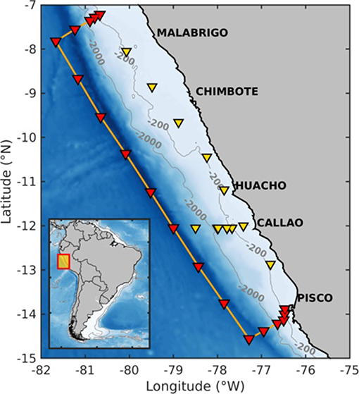
Figure 1. Hydrographic casts in the study region over a bathymetric map of Peru. Yellow and red triangles depict stations with water sampling for chemical analysis, while the yellow line indicates the main offshore transect.

Discrete samples for DIC and pH analysis were collected over depth gradients at coastal and offshore sites in the Peruvian OMZ area. A total of 31 station profiles of ~500 meters depth were generated. At each station, vertical profiles were produced using standard oceanographic equipment (CTD-rosette at most stations). Seawater samples for DIC and pH samples were collected by a rosette casts covering the low-oxygen water with an average of 12 depths targeting the key water column features of the oxic photic zone, oxycline (upper), OMZ interface, and anoxic OMZ core.

Water samples for DIC analysis were collected in 250-ml sodium borosilicate bottles and preserved with 50 μl of HgCl₂ saturated solution. For pH analysis, the samples were collected directly from the Niskin bottles using 60-ml syringes. All samples were analyzed aboard the ship. For DIC analysis, a LI-7000 gas analyzer (CO₂/H₂O, LICOR, Lincoln, NE, USA) was used. The certificate reference material for DIC analysis was provided by the laboratory of Dr. Andrew Dickson of Scripps Institution of Oceanography (Dickson et al., 2003). The relative difference averaged ±2 μmol kg⁻¹ (0.2% error).

The pH was measured using a glass electrode at 25°C on the seawater scale (pHsw) as described by Chapa-Balcorta et al. (2015). We use the program CO2SYS (Lewis and Wallace, 1998) and DIC-pH_sw to calculate pCO₂, in situ pHsw, and the aragonite saturation state (Ω_Arg). We use the constants proposed by Mehrbach et al. (1973) for these calculations. The uncertainty obtained for in situ pH_sw, Ω_Arg, and pCO₂ was ± 0.04 ± 0.2, and 56 μatm, respectively. The pCO₂ variability range observed in Peruvian waters was 25-fold greater than the error.

Wind Data

Wind speed data were obtained from the SeaWinds database provided by NOAA (Zhang et al., 2006a,b). Wind stress was computed using the bulk equation (Schwing et al., 1996). Monthly means of the wind speed field were also derived from the Copernicus level 4 multi-sensor blended wind product.

Vertical Velocities Due to Wind Stress Curl and Ekman Transport

The curl-driven vertical velocities (w_c) and coastal upwelling associated with Ekman offshore transport (w_e) at the limit of the mixed layer were estimated following Rykaczewski et al. (2015) using Equations (1) and (2):

$\begin{array}{llll}{w}_c& =& \frac{1}{{\rho }_{w}f}{\nabla }_h\times \tau & (1)\end{array}$

$\begin{array}{llll}{w}_e& =& \frac{{\tau }_a}{{\rho }_{w}fRd}& (2)\end{array}$

where ρ_w = 1,024 kg m3 is the seawater density, f is the coriolis parameter, τ is the wind stress vector field, τ_a is the wind stress parallel to the coastline, and Rd is the local Rossby radius of deformation. Note that using Rd to convert Ekman transport in upwelling rate yields an estimate that is in the low range values of the actual amplitude of vertical velocity since the upwelling scale is smaller than Rd [cf. Marchesiello and Estrade (2010)].

Variability of Sea Surface Height Anomalies

In order to calculate the relative importance of the different scales of variability for sea surface height anomalies (SSHa) in the study area, the seasonal, interannual, and mesoscale signals were derived following the methods of Godínez et al. (2010) and León-Chávez et al. (2015). A 21-year database (1993–2014) of mean SSHa distributed by AVISO was used (http://www.aviso.altimetry.fr).

The seasonal, mesoscale, and interannual signals were separated. The first was obtained using a harmonic fit, while the second and third were obtained by means of orthogonal empirical functions (Equations 3 and 4).

$\begin{array}{l}SSHa(\overrightarrow{\text{x}},\text{t})={\text{A}}_a(\overrightarrow{\text{x}})cos(\omega \text{t}-{\phi }_a(\overrightarrow{\text{x}}))+{\text{A}}_s(\overrightarrow{\text{x}})cos(2\omega \text{t}-{\phi }_s(\overrightarrow{\text{x}}))\\ +{\text{F}}_1(\overrightarrow{\text{x}}){\text{f}}_1(\text{t})+{\displaystyle \sum _{n=2}^N}{\text{F}}_n(\overrightarrow{\text{x}})f_n(\text{t})& (3)\end{array}$

$\begin{array}{l}SSHa(\overrightarrow{\text{x}},\text{t})=SSH{a}_{season}(\overrightarrow{\text{x}},\text{t})+SSH{a}_{inter}(\overrightarrow{\text{x}},\text{t})\\ +SSH{a}_{meso}(\overrightarrow{\text{x}},\text{t})& (4)\end{array}$

A_a and A_s are the annual and semi-annual amplitudes of the harmonic fit, respectively, while $\overrightarrow{x}$ is the spatial vector, φ_a and φ_s are the annual and semi-annual phases, ω is the annual radian frequency, t is the time referred to the beginning of the year, and n is the number of EOF. The first two terms on the right of Equation (3) are the seasonal components (SSHa_season is the first term in Equation 4), which were calculated using a least squares fitting. Fitting errors and uncertainties were calculated as in previous studies (Prentice et al., 2001; Ripa, 2002). $F_1(\overrightarrow{x})$ and f₁(t) are the spatial and temporal series of the first EOF mode, which in the South Equatorial Tropical Pacific (SETP) typically contain the interannual signal (SSHa_inter in Equation 4) that is characterized by ENSO-induced variability (Macharé and Ortlieb, 1993). In the last term of Equation (3), $F_n(\overrightarrow{x})$ and f_n(t) are the spatial and temporal series of the nth EOF mode. The sum of these (2 to N) mainly contains mesoscale variability (SSHa_meso, third term of Equation 4), although it may include some interannual variability not captured by the first EOF. Analyzing this information enables us to identify the dominant processes in the region in general as well as during the time of our cruise, allowing us to weigh the significance of the measurements according to the predominant signal type. The local variance (LV) of each variability component (seasonal, interannual, and mesoscale) was calculated as follows:

$\begin{array}{ll}L{V}_{season}=\frac{{\sigma }_{SSH{a}_{season}}^2*100}{{\sigma }_{SSHa}^2}& (5)\end{array}$

where LV_season indicates local variance, ${\sigma }_{SSH{a}_{season}}^2$ is the variance of the seasonal component of SSHa, and ${\sigma }_{SSHa}^2$ is the variance of the original SSHa. LV was calculated per pixel for each time series. The same procedure was used for the interannual and mesoscale components. The complete series was used for this calculation (1992–2015). The signal decomposition during the cruise was obtained by reconstructing SSHa data of the separated variability scales for the dates corresponding to the sampling periods. The seasonal data were reconstructed from the harmonic analysis. The interannual data were reconstructed from the first EOF. The mesoscale data were constructed from the sum of the EOF from 2 to N.

Inferred Sea Surface Height Anomalies

With a deep level of no motion in the offshore transect (1,000 db), we used T and S to calculate density and thus inferred sea surface height anomalies, which we compared to the AVISO satellite product. The dynamic height calculation was performed using the functions of the TEOS-10 library (McDougall and Barker, 2011). The measured salinity and temperature data were interpolated vertically with an interval of 1 m using the objective interpolation of Barnes (1964).

Results

We provide a description of the circulation patterns that drive the physical and biogeochemical patterns observed in the study region during the cruise, and we use this as a frame of reference to define the importance of each water mass in the region. We also provide a description of the oceanographic conditions during the cruise, which is interpreted considering the analysis of altimeter data to estimate anomalous conditions in seasonal and interannual timescales.

Wind, Wind Stress Curl, and Ekman Transport Conditions

At the beginning of the sampling period in January 2014, the wind speed was <5 m s⁻¹ throughout the coastal area spanning from Pisco to Malabrigo. The wind speed was stronger offshore and presented values of 6–7 m s⁻¹ (Figures 2A,B). The most intense winds 10 m s⁻¹ were observed offshore in February, although winds of 7 m s⁻¹ were observed in the coastal region near Pisco. During the January sampling period, the winds oscillated from ~3 to 5 m s⁻¹ and produced relatively weak upwelling compared to the remainder of the period (Figure 2C). Stronger yet opposite wind stress can be observed in February (Figure 2D). The combination of calm (Figure 2A) and subsequently strong winds (Figure 2B) produced different oceanographic conditions; namely, regions with high vertical mixing and areas with coastal upwelling (Figure 3). The mean vertical velocities associated with Ekman transport and the monthly vertical transport means due to winds stress curl for January and February are presented in Figure 3. Of note, February presented the highest Ekman offshore transport and vertical transport values. However, the vertical transport in front of Chimbote did not occur because of the presence of an anticyclone eddy (Figure 4).

FIGURE 2

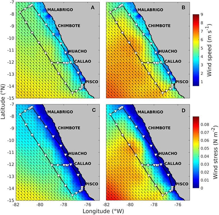
Figure 2. Wind speed data were obtained from the NOAA SeaWinds database. The upper panels show the January (A) and February (B) 2014 monthly mean of the wind speed field derived from the Copernicus level 4 multi-sensor blended wind product. Lower panels show wind stress field monthly mean for January (C) and February (D) 2014.

FIGURE 3

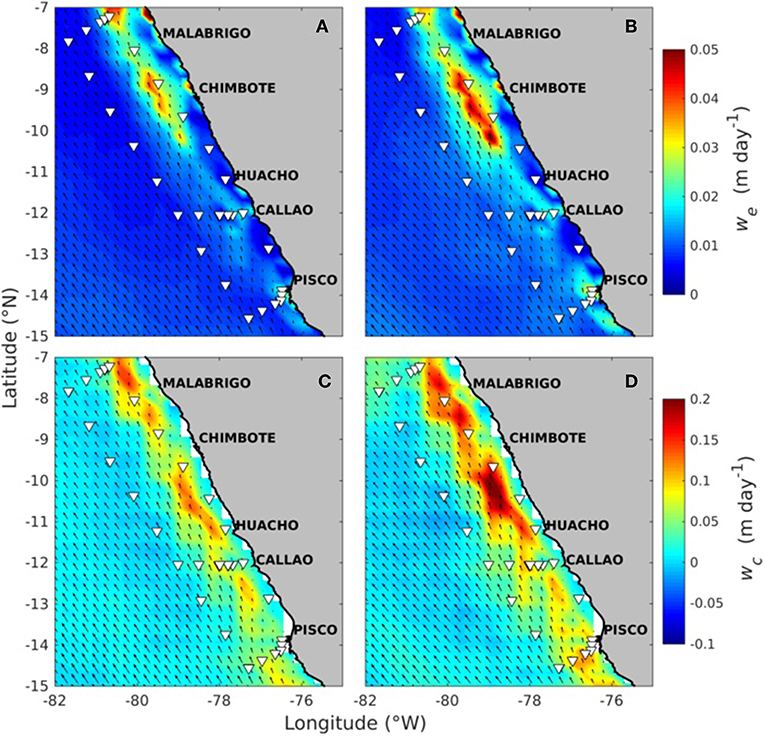
Figure 3. The (A,B) show the mean vertical velocities associated with Ekman transport (w_e) for January and February, respectively (upper color scale). In the lower panels, monthly vertical transport (w_c) means due winds stress curl are shown (lower color scale) for January (C) and February (D). For all the panels in this figure, the black arrows represent the mean wind stress vectors for the respective month.

FIGURE 4

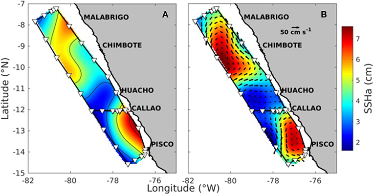
Figure 4. (A) shows objectively interpolated SSHa values at the sampling date in a given position. (B) shows February 2014 mean SSHa in the color scale, and the black arrows represent the mean geostrophic velocity (cm s⁻¹).

Variability in Sea Surface Height Anomalies

The SSHa in the study area for January and February 2014 are shown in Figure 4. The cruise track variability that was attributed to mesoscale eddies during February was present during the anticyclonic eddy from Malabrigo to the middle of Huacho for both odd shore and coastal stations. In front of Huacho and to the north of Callao, cyclonic eddy influence may be observed in both January and February (Figures 4A,B). While the effect of each of the conditions on the chemistry of the CO₂ system will be described later, the spatial distribution of the CO₂ variables was directly associated with the various oceanographic conditions.

Water Masses, Water Types, and Vertical Structure

The distribution of water masses was examined to analyze the potential effects on the carbonate chemistry in the study area. We also found it very useful to study the water-type distribution because of the broad T-S variability. The T-S plot in Figure 5 incorporates several characteristics for comparison on the Z axis, such as latitudinal distribution, oxygen concentration, pH_SW, pCO₂, and omega aragonite (Ω_Arg). The T–S diagrams for all sections in the study area indicate the presence of four water masses in the first 500 m based on the classifications of Silva and Neshyba (1976); Silva et al. (2009). In addition, three water types were observed as defined by the conditions of Swartzman et al. (2008). The water masses that were detected were Subtropical Surface Water (SSW), Equatorial Subsurface Water (ESSW), Antarctic Intermediate Water (AAIW), and Pacific Deep Water (PDW). The water types that were observed were Cold Coastal Water (CCW); Mixed Equatorial, Subtropical and Coastal Water (MESC); and Coastal Antarctic Water (CAW). The CAW reported by Swartzman et al. (2008) was detected as a small intrusion between 55 and 80 m.

FIGURE 5

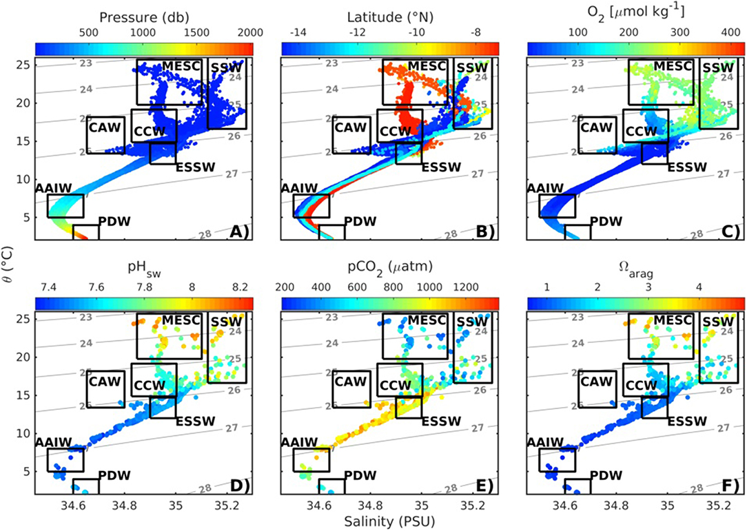
Figure 5. Potential temperature and salinity diagram for the cruise. The color bar for each plot indicates (A) depth, (B) latitude, (C) oxygen, (D) pH_SW, (E) in situ pCO₂, and (F) omega aragonite. The water masses were detected based on the criteria of Silva and Neshyba (1976) and were Surface Subtropical Water (SSW), Equatorial Subsurface Water (ESSW), Antarctic Intermediate Water (AAIW), and Pacific Deep Water (PDW). The observed water types observed were Cold Coastal Water (CCW); Mixed Equatorial, Subtropical and Coastal Water (MESC); and Coastal Antarctic Water (CAW). CAW was reported by Swartzman et al. (2008).

In surface waters, MESC and SSW were detected in the first 25 m (Figure 5A). MESC is less salty and it was located north of 8°N, while SSW had salinities >35 and was observed south of 12°N (Figure 5B). The corresponding MESC values following 24 kg m⁻³ isopycnal (located in <10 m) for oxygen, pH, pCO₂, and Ω_arag were 250 μmol Kg⁻¹, ~8.1, <500 μatm, and >3.5 units, respectively. The values for SSW between 10 and 60 m for the 25 kg m⁻³ isopycnal were >200 μmol Kg⁻¹, >7.8, ~550 μatm, and >2.0 units (Figure 5). CCW located below MESC was also found at 8°N between 20 and 60 m depth (Figures 5A,B). When following the 25 kg m⁻³ isopycnal in <20 m depth, the average values of CCW characteristics indicated that this water type presented less oxygen, lower pH, higher pCO₂, and lower Ω_arag (close to zero to 50 μmol Kg⁻¹, ~7.7, <1,000 μatm, and <2.0, respectively) when compared to that of MESC. The water type CAW was observed between 55 and 80 m. This water mass presented the lowest oxygen concentrations, low pH, higher pCO₂, and low Ω_arag (0 and 20 μmol kg⁻¹, ~7.7, >1,300 μatm, and <2.0, respectively). In subsurface waters, the main water mass of the OMZ and CMZ in the study area considering the observed characteristics (low oxygen and pH and high pCO₂ and DIC) was ESSW. The upper ESSW limit presented a potential density anomaly of 26 kg m⁻³ (Figure 5) in the offshore transect, and this isopycnal was found at ~70 m depth (Figure 6). However, the isopycnal was found at ~30 m near the coast at 14°S. The oxygen concentration declined to <20 μmol kg⁻¹ at this depth but also presented pH values of 7.7 and <1.5 units for Ω_arag (Figure 6).

FIGURE 6

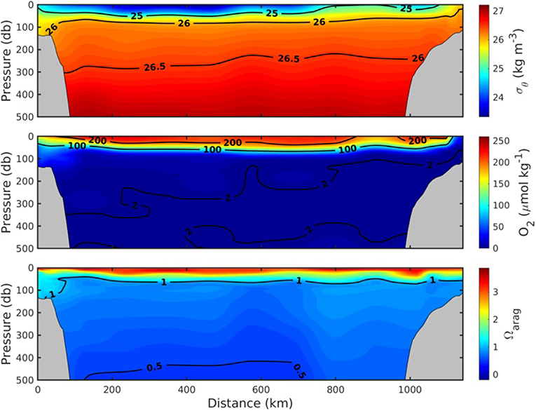
Figure 6. Vertical distribution of the potential density anomaly (σ_θ, kg/m³), dissolved oxygen (DO, μmol kg⁻¹), and omega aragonite (Ω_arag) along the transect.

Figure 7 presents the spatial distribution at 30 m for temperature, density, oxygen, pCO₂, pH, and omega aragonite. With the exception of a few stations located in the offshore region between 8 and 11°S, the area was influenced by subsurface waters and was therefore characterized by low concentrations of oxygen (<10 μmol kg⁻¹), subsaturation values of omega aragonite (~1 near the coast Callao-Pisco), low pH (<7.5), and high pCO₂ (values from ~ 500 to 1,200 μatm). The highest values of pCO₂ were observed in the coastal region between Callao and Pisco at the southern end of the transect.

FIGURE 7

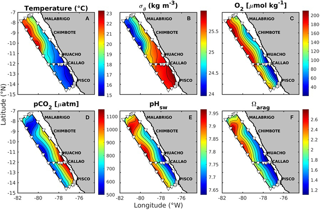
Figure 7. Surface distribution maps of physical and chemical variables at 30 m depth. Top panels show (A) temperature, (B) density, and (C) oxygen. Bottom panels show (D) derived in situ pCO₂ (pH-DIC), (E) in situ pH_SW, and (F) omega aragonite (Ω_arag).

Vertical Mixing

Two different oceanographic scenarios were found during the cruise and consisted of the presence or absence of upwelling. The wind stress near the coast was low during January (<0.03 N m⁻²) prior to sampling (Figures 2, 3) and presented wind speed values <3 ms⁻¹. However, in February, the monthly wind speed mean was 7 ms⁻¹ while the wind stress was ~0.07 N m⁻². In February we found the highest values for both Ekman offshore transport and vertical transport (Figure 3). During February, the upper ESSW limit was found near the surface between 20 and 50 m depth in the coastal area between 12 and 14°S. The lowest surface temperatures (~17°C), lower oxygen concentrations (<100 μmol kg⁻¹), the highest surface DIC concentrations (~2,300 μmol kg⁻¹), and low omega aragonite values (<1.5) were present at ~20 m depth (Figure 8).

FIGURE 8

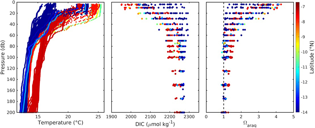
Figure 8. Profiles of temperature (°C), dissolved inorganic carbon (DIC), and omega aragonite (Ω_arag). The color bar represents the latitude for all of the plots and the black dashed line for omega aragonite indicates the saturation value (Ω_arag = 1).

During the cruise, weakly stratified regions were identified based on temperature profiles with a N-S gradient (Figure 8). The stratification parameter was calculated according to Simpson (1981) for the upper 300 m of the water column. This value expressed in J m⁻³ and represents the amount of work per volume that is needed to mix the water column to a specified depth. The lowest stratification values were detected (<200 J m⁻³) between 11 and 15°S near the upwelling area found between Callao and Pisco (see vertical profiles in Figure 8). However, higher stratification values (>400 J m⁻³ were found between 8 and 11°S. For all sampled areas, the calculated stratification average was 350 J m⁻³. This combination of upwelling and stratification plays an important role in the spatial and vertical distribution of DIC, omega aragonite, oxygen, and temperature.

Circulation Based on SSHa Variability Scales

The decomposition of SSHa variability for the Peruvian area based on 21 years of AVISO data shows that the interannual signal is dominant (~30–80%), followed by the mesoscale signal (20–60%), and finally the seasonal signal (~7 and 30%; Figure 9). However, the cruise took place during a normal year. The seasonal cycle presented weak variance, which is consistent with previous studies in the eastern tropical Pacific (Takahashi et al., 2011).

FIGURE 9

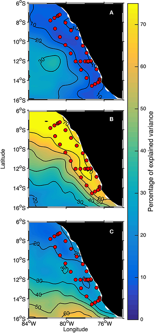
Figure 9. Variance of the sea level anomaly for the three time scales: (A) seasonal, (B) interannual, and (C) mesoscale.

Seasonality between 6 and 16°S had a greater effect on SSHa between 80 and 84°W in offshore areas while a small influence was observed near the coast between 8 and 13°S, which coincides with the location of the sampling network (Figure 9A). The interannual variability was mainly the result of ENSO as shown in Figure 9B where the temporal component of the first mode (EOF1) can be seen to be correlated with the El Niño multivariate (MEI) and ONI indices. It should be noted that the region is partially located within the area referred to as El Niño region I (Trenberth and, 2019). Figure 9B also shows that the ENSO effect extended south of the study area near the coast with a local variance between 57–77%.

Mesoscale eddy activity is generated by variations in density that arise from coastal currents in their own vortices. The greatest effect of this activity was detected with SSHa in the southern region between 13 and 16°S, although mesoscale eddy activity presented latitudinal variation and minimum values were present in the northern region (Figure 9C). This is likely because most eddies are generated near the coastal region between 10–16°S and reach their greatest diameters between 13–16°S.

During neutral El Niño conditions, as in February 2014, the ENSO signal may be overshadowed by high mesoscale variability. The signal decomposition for the sampling dates during the cruise is shown in Figure 10. January and February were neutral ENSO periods (ONI = −0.4), and the interannual signal was weak (0.5–1.8 cm). The strongest driver of SSHa variability was the mesoscale signal (−5.9 to 5.1 cm), which was mainly due to the presence of eddies, with fluctuations of −1.3 to 3.0 cm generated by seasonality.

FIGURE 10

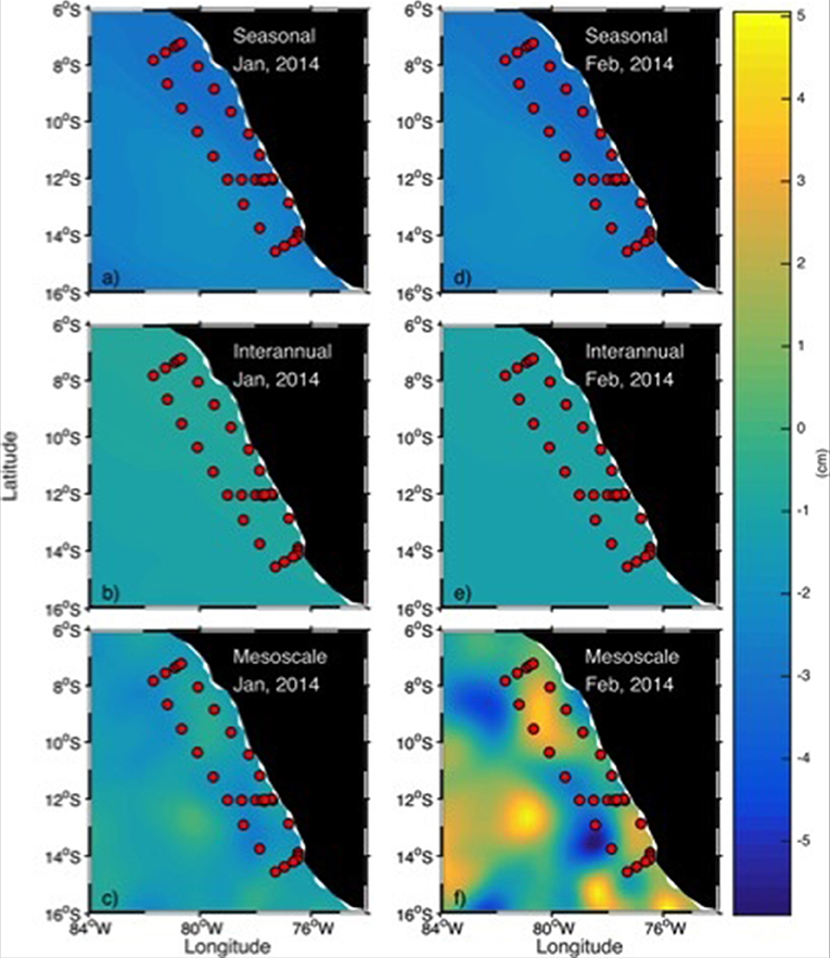
Figure 10. Signal decomposition for January and February: (a,d) seasonal, (b,e) interannual, and (c,f) mesoscale.

Inferred Sea Surface Height Anomalies, Satellite Product, and Cruise Track Variability Attributed to Mesoscale Eddies

To evaluate if mesoscale eddy activity played a large role in carbon system variability within the inner and outer transects, two approaches were considered. Inferred SSHa by calculate density and thus to compare with the satellite product (Figures 11A,C,D). We found that both estimations showed similar trends. However, a linear regression analysis was carried out to determine if the inferred SSHa were associated with the satellite dynamic height product. The R² value of this analysis was 0.78. Likewise, a statistically significant Pearson linear correlation coefficient of r_p = 0.88 was obtained, indicating that increases in sea surface height were associated with SSHa (confidence level of 95%).

FIGURE 11

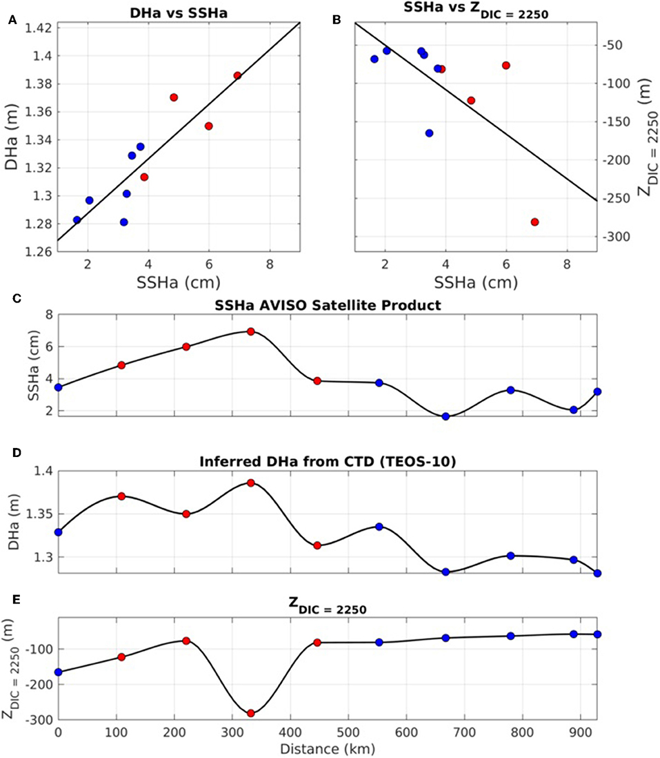
Figure 11. (A) Association between DHa and SSHa for the deepest points of the main offshore transect (see Figure 1). The black straight line corresponds to the linear model obtained with x₀ = 1.25, x₁ = 0.02, R² = 0.78, and r_p = 0.88. (B) Association between Z_{DIC = 2250} (depth at which DIC = 2,250 μmol/kg) and SSHa for the deepest points of the main offshore transect. The black straight line corresponds to the linear model obtained with x₀ = −29.11, $x_1=8.08,R^2=0.46$, and r_p = −0.68. From (C–E) we show the values of SSHa, DHa, and Z_{DIC = 2250} from the deepest points of transect 1. The horizontal axis corresponds to distance (km), beginning from the North (0 km).

After SSHa were estimated, they were used to geo-reference each carbonate system profile to determine the degree of variability in the carbonate system that may be attributed to mesoscale eddies (Figures 11B,E). For example, the large horizonal and vertical variability associated with DIC values of 2,250 μmol kg⁻¹ was due to eddy presence. The linear regression was performed considering SSHa and DIC depth (Z). An association was found between Z_{DIC = 2250} (depth at which DIC = 2,250 μmol kg⁻¹) and SSHa for the deepest portions of the main offshore transect. The model obtained has x₀ = −29.11, x₁ = 8.08, R² = 0.46, and r_p = −0.68. We found that mesoscale processes change the upper depth limit of ESSW and the depth of this water mass, while affecting DIC, the aragonite saturation depth, and the upper limit of the OMZ.

Discussion

This study describes the Peruvian upwelling conditions observed during January and February 2014 and the associated spatial variation of the CO₂ system. During upwelling events, the aragonite saturation depth was observed to be close to 50 m, but values of <1.2 were detected close to 20 m and were accompanied by low pH (<7.5), high pCO₂ (>1,250 μatm), and high DIC (>2,250 μmol kg⁻¹). These chemical characteristics were linked with the portion of the water-column that spanned from the upper limit of Equatorial Subsurface Water (ESSW) to the upper limit of the OMZ (<5 μmol kg⁻¹) and the carbocline (~2,300 μmol kg⁻¹). Our analysis of the decomposition of SSHa variability also shows that the coastal-oceanic signal was dominated by interannual variability. However, during our sampling period, mesoscale processes were key drivers of surface water dynamics. In particular, the upper depth limit of ESSW may be altered by physical phenomena, such as eddies or interannual events. This results in changes in the depth of this water mass and affects DIC, the aragonite saturation depth, and the upper limit of the OMZ.

Vertical Mixing, Water Masses, and Water Types

Large spatial variability in sea surface anomalies were found (Figure 4). Part of this variability may be attributed to the influence of mesoscale eddies, which modify biogeochemistry. For example, shallower saturation horizons and high DIC values may be due to cyclonic eddy activity, while low DIC concentrations will be deeper due to anticyclonic eddy activity. The sampling area showed eddy production in the oceanic region, which may account for a large percentage of the variability that was observed in the offshore stations located south of 13°S (>40%) as may be seen in Figure 9C. Additional information regarding the effect of eddies on the biogeochemistry inside an OMZ has been reported by Bettencourt et al. (2015) who indicate that mesoscale structures have relevant dual roles at depths between 380 and 600 m. Firstly, their mean positions and paths delimit and maintain the boundaries of oxygen minimum zones. Secondly, their high frequency fluctuations entrain oxygen across these boundaries. As a result, these eddy fluxes contribute to the ventilation of the oxygen minimum zone. Eddy structures can introduce water types with different pH and Ω_arag values (Figure 5). For example, MESC and SSW at the surface were affected by anticyclonic and cyclonic eddies (Figure 6), respectively, and MESC had higher pH and oxygen values than SSW (Figure 5).

The offshore surface waters were saturated with regard to aragonite (Ω_arag >1.5 to >4.5) in the first 50 m of the water column (Figures 6, 7). However, for depths below 150 m, the Ω_arag values were <1. These values are similar to those reported for the open ocean (300 km from the coast) in the Eastern South Pacific (Feely et al., 2012; Jiang et al., 2015). The upper limit of ESSW can be identified by the 26 kg m⁻³ isopycnal (Figure 5). The depth of this isopycnal surface was closely related to the thermocline and with the aragonite saturation horizon (Figure 6). Therefore, most of the chemical features associated with this isopycnal were similar regardless of depth. In most cases, the sinking of this density surface directly resulted in changes in the depth of the aragonite saturation horizon. Near Pisco, the upper limit of ESSW was as shallow as ~20 m depth.

During the cruise, the low surface Ω_arag values (<1.2) that were observed near the coastal stations were due to the influence of upwelled water. However, a cyclonic eddy was present during sampling along the coast between 11 and 12°S (Figure 4; February). This eddy resulted in an upward vertical transport of aragonite-undersaturated ESSW, which reduced the surface values of Ω_arag (Figures 6, 7). Furthermore, an anticyclone was observed in most of the oceanic region (8–12°S and 80–81°W) that resulted in a depression of the aragonite saturation horizon. The highest Ω_arag values (near 3) that were found in the Peruvian area were observed offshore in the northern transects. Nevertheless, the high offshore pH values (>8.1) and low pCO₂ values (<600 μatm) that were found in this region suggest that the aragonite saturation state is driven by two processes: outgassing of CO₂ and the biological consumption of dissolved inorganic carbon. However, submesoscale processes are another physical driver of CO₂ outgassing. Köhn et al. (2018) carried out a CO₂ variability study across an upwelling front near Peru using high-resolution underway measurements and provided evidence of the complex submesoscale distribution of surface CO₂ in the Peruvian upwelling system. Thus, physical processes may also influence the distribution of pCO₂ on different spatial and time scales.

Spatial Variability

In winter, the Peruvian Coastal Current (PCC) flows intensely toward the equator, while the Peruvian Coastal Under Current (PCUC) flows toward the pole (Bakun and Nelson, 1991; Penven et al., 2005; Croquette et al., 2007; Ayón et al., 2008; Dewitte et al., 2011). During normal conditions, upwelling transports water from the PCUC (Ayón et al., 2008; Montes et al., 2011). During La Niña conditions, the Cold Coastal Water (CCW) water type is heavily influenced by upwelling (Ayón et al., 2008; Montes et al., 2011).

Based on the analysis of 1993–2014 SSHa data, we found that interannual variability plays the most important role (up to 60% of local SSHa variance) in determining the circulation of the coastal areas and in the southern region of our study area, followed by mesoscale variability. This result is different from what was observed by Godínez et al. (2010) for the OMZ located in the Eastern Tropical Pacific (ETP) off the coast of Mexico (15–24°N). In their study, seasonality was found to be the dominant signal, which was followed by the mesoscale signal. The mesoscale contribution to SSHa variability was four times larger than what was observed for the ETP (10–20% of the local SSHa variance). In contrast with our study area, interannual variability was three times larger than mesoscale variability near the coast. The waters off Peru are intimately associated with the dynamics of the equatorial Pacific and are thus subject to large temporal variations. The ENSO cycle, with its warm El Niño phase and cold La Niña phase, is comprised of a natural interannual oscillation frequency of the ocean-atmosphere system in the tropical Pacific (Takahashi et al., 2011). Over several months, this cycle substantially alters the functioning of ecosystems associated with the coastal outcrop (Grados et al., 2018).

In our study, mesoscale variability was less important than interannual variability, but we also found that mesoscale eddy activity notably influenced carbon system variability within the inner and outer transects (Figure 11). We found that the large spatial variability observed in our study area was attributed to the influence of mesoscale eddies, which can modify the distribution of biochemical variables, such as the aragonite saturation horizon, in response to shallower (cyclonic eddies) or deeper (anticyclonic eddies) thermoclines. According to Willett et al. (2006), eddies are the main contributors of mesoscale variability in the ETP. Eddies affect the spatial distribution of dissolved chemicals by Ekman pumping and by exporting dissolved and particulate materials into the open ocean, fostering horizontal advection (Chen et al., 2007; Samuelsen and O'Brien, 2008; Gaube et al., 2014; Nagai et al., 2015). In the study area, mesoscale processes influenced the upper depth limit of ESSW, changing the depth of this water mass and affecting DIC, aragonite saturation, and the OMZ depth. Mesoscale eddies, whether they are driven by wind forcing or otherwise, can persist for weeks (cyclonic) or months (anticyclonic; Gonzalez-Silvera et al., 2004; Palacios and Bograd, 2005). Although mesoscale processes were not as important as interannual processes, they were still very important in the region during the cruise and affected the spatio-temporal variability of the biogeochemical patterns in the region and are thus key factors to consider when studying the carbonate system in the ocean offshore of Peru.

Variability of Dissolved Inorganic Carbon

The DIC concentrations detected in the study area were within the data ranges that have been reported for SSW in the ETP (Paulmier et al., 2011; Franco et al., 2014; Chapa-Balcorta et al., 2015). The DIC variability observed during sampling indicates that upwelling and mesoscale variability affect DIC values. The corresponding changes in pCO₂ and Ω_arag affected both regional biogeochemical conditions and habitat quality for calcifying or pH-sensitive species.

The impact of climate change on the dynamics of the Eastern Boundary upwelling system (EBUS) has been debated and a consensus has not been reached so far, mostly because of competing effects due to the increase in upwelling favorable winds induced by the expansion of the Hadley cell (Bakun et al., 2015; Rykaczewski et al., 2015) and the increase in surface warming that increases vertical stratification and tends to reduce upwelling (e.g., Echevin et al., 2012 for the coast of Peru). There is also uncertainty with regard to whether upwelling favorable winds will actually increase in the mid-latitudes (Goubanova et al., 2011) given that increasing trends in alongshore favorable winds are barely detected in existing data sets (e.g., Figure 1 of Belmadani et al., 2014). It has been postulated that along the Peruvian coast, global warming has increased the heat difference between the continent and the adjacent sea. This change has resulted in an intensification of the winds, which has resulted in the coastal outcrop. However, recent studies suggest a notable cooling of the marine-coastal strip between central Peru and northern Chile over the last 35 years, although records of coastal winds are scarce and the causes behind this trend remain unclear (Yáñez et al., 2018). The first simulations of climate change effects in the waters off Peru predicted a decrease of the coastal outcrop, an intensification of coastal retention processes, and a reduction in marine productivity, in which thermal stratification plays an important role (Gutiérrez et al., 2011). These changes in upwelling intensification will also be reflected in the carbon biogeochemistry of coastal areas.

Aragonite Saturation Horizon Maintenance

A lower oxygen concentration at the aragonite saturation depth was found in the southern stations near the coastline (Figures 6, 7). The remineralization of organic matter produced at the surface may intensify the consumption of oxygen in the subsurface layer due to low ventilation driven by strong stratification in the area (Fiedler and Talley, 2006; Fiedler et al., 2013; Franco et al., 2014). The latter is consistent with what was reported by Fiedler and Talley (2006), who concluded that 90% of organic matter was remineralized in the first 200 m of the water column. In turn, Paulmier et al. (2006) showed that organic matter remineralization in the oxycline of the Humboldt system was 3-fold more intense than in the core of the OMZ, which favors the maintenance of these zones. In highly productive coastal zones, eutrophication due to runoff from terrestrial nutrient addition may have a greater effect on the decrease of aragonite saturation than on ocean acidification driven by anthropogenic CO₂ absorption (Borges and Gypens, 2010). Water with low oxygen and carbonate ion concentrations may have different biological responses, as this situation may lead to habitat increases or decreases for the species that reside in OMZs, particularly because these chemical environments affect their metabolic functions.

Like biological processes, physical drivers play a very important role in the vertical distribution of several CO₂ variables in the ocean. The results reported in this study clearly demonstrate that DIC concentrations, pCO₂, and Ω_arag depend not only on the upwelling season but also on the presence, absence, and intensity of mesoscale eddies. Therefore, proper evaluations of physical drivers should always include an analysis of the indicators of these eddies, such as dynamic height, geostrophic currents, or altimetry in models that are able predict which areas are likely to experience ocean acidification.

The upwelling system in Peru is a natural laboratory for the study of regional interactive processes between the land, ocean, and atmosphere while providing a unique opportunity to understand carbon variability in different scales. For example, the Peruvian anchovy Engraulis ringens lives and spawns in a region where pCO₂ values may be higher than 1,000 ppm (Friederich et al., 2008), and low survival rates have been attributed to these high values (Shen et al., 2017). These authors also highlight the need to understand the effect of pCO₂ levels on spawning and mortality rates to predict the effects of ocean acidification on fisheries management. In response to future warming, changes in timing, intensity, and spatial heterogeneity are expected to occur in most EBUS (Wang et al., 2015).

Conclusions

During the upwelling events, the aragonite saturation depth was observed to be close 50 m, but values <1.2 were detected close to 20 m along with low pH (<7.5), high pCO₂ (>1,250 μatm), and high DIC (>2,250 μmol kg⁻¹) values. These chemical characteristics were associated with Equatorial Subsurface Water (ESSW). In addition, the aragonite saturation depth became gradually shallower from north to south, beginning at 140 m and decreasing to <40 m with pCO₂ values close to 1,250 μatm.

Large spatial variability in surface values was also observed. Part of this variability can be attributed to the influence of mesoscale eddies, which can modify the distribution of biogeochemical variables. The results reported here clearly demonstrate that DIC concentrations, pCO₂, and Ω_arag depend not only on upwelling but also on the presence, absence, and intensity of mesoscale eddies. Mesoscale eddies changed the upper depth limit of ESSW, changing the depth of this water mass and affecting DIC, aragonite saturation, and OMZ depth.

Our analysis of the decomposition of SSHa variability that was based on a 21-year data set, indicated that the interannual signal was the dominant coastal-oceanic signal. However, during our sampling period, mesoscale processes were key drivers of surface water dynamics. The 2014 cruise was characterized by weak Kelvin activity, and physical forcing was more associated with eddy activity. Large spatial variability at the surface was also found. Part of this variability was attributed to the influence of mesoscale eddies which modify biochemistry. For example, the aragonite saturation horizon was affected by shallower or deeper thermoclines, which were the result of cyclonic or anticyclonic eddies, respectively. Near the coast and south of 12°S, pH_T values from 8 to 7.6 were observed in upwelling zones but were also distributed in several shallow water types. Values <1.2 were detected close to 20 m along with low pH (minimum of 7.5), high pCO₂ (maximum of 1,250 μatm), and high DIC concentrations (maximum of 2,300 μmol kg⁻¹). Weighing the relative importance of each individual signal leads to a better understanding of the biogeochemical processes in the area.

Author Contributions

The conceptualization and arrangement of the original manuscript was under the charge of JH-A, AP, and VG. The conceptual design and financial support of the oceanographic expeditions were under the direction of VG, AP, BD, and CM. All CTD data were facilitated through JS. Preprocessing of all data was carried out by CC-B, JS, IM, GD, and MB. Laboratory analyses were conducted by JH-A. All authors contributed equally to the original manuscript.

Funding

AMOP project was supported by IRD, CNRS/INSU, LEGOS.

Conflict of Interest

The authors declare that the research was conducted in the absence of any commercial or financial relationships that could be construed as a potential conflict of interest.

Acknowledgments

We wish to thank the crew of the French R/V Atalante during the cruise in the framework of the AMOP project (Activity of research dedicated to the Minimum of Oxygen in the eastern Pacific). We also thank Sergio Larios for his input in the data processing.

Sea surface level anomaly data were produced by Segment Sun Altimetrie et Orbitographie/Developing Use of Altimetry for Climate Studies (Ssalto/Duacs) and distributed by Archiving Validation. The interpretation of satellite Oceanographic Data (Warning) was carried out with the support of the Center National d'Etudes Spatiales (CNES).

References

Ayón, P., Criales-Hernandez, M. I., Schwamborn, R., and Hirche, H.-J. (2008). Zooplankton research off Peru: a review. Prog. Oceanogr. 79, 238–255. doi: 10.1016/j.pocean.2008.10.020

CrossRef Full Text | Google Scholar

Bakun, A., Black, B. A., Bograd, S. J., García-Reyes, M., Miller, A. J., Rykaczewski, R. R., et al. (2015). Anticipated effects of climate change on coastal upwelling. Ecosystems 1, 85–93. doi: 10.1007/s40641-015-0008-4

CrossRef Full Text | Google Scholar

Bakun, A., and Nelson, C. S. (1991). The seasonal cycle of wind stress curl in sub-tropical eastern boundary current regions. J. Phys. Oceanogr. 21, 1815–1834. doi: 10.1175/1520-0485(1991)021<1815:TSCOWS>2.0.CO;2

CrossRef Full Text | Google Scholar

Barnes, S. L. (1964). A technique for maximizing details in numerical weather map analysis. J. Appl. Meteorol. 3, 396–409. doi: 10.1175/1520-0450(1964)003<0396:ATFMDI>2.0.CO;2

CrossRef Full Text | Google Scholar

Belmadani, A., Echevin, V., Codron, F., Takahashi, K., and Junquas, C. (2014). What dynamics drive future wind scenarios for coastal upwelling off Peru and Chile? Clim. Dyn. 43, 1893–1914. doi: 10.1007/s00382-013-2015-2

CrossRef Full Text | Google Scholar

Bettencourt, J. H., López, C., Hernández-García, E., Montes, I., Sudre, J., Dewitte, B., et al. (2015). Boundaries of the peruvian oxygen minimum zone shaped by coherent mesoscale dynamics. Nat. Geosci. 8, 937–940. doi: 10.1038/ngeo2570

CrossRef Full Text | Google Scholar

Borges, A. V., and Gypens, N. (2010). Carbonate chemistry in the coastal zone responds more strongly to eutrophication than to ocean acidification. Limnol. Oceanogr. 55, 346–353. doi: 10.4319/lo.2010.55.1.0346

CrossRef Full Text | Google Scholar

Bretagnon, M., Paulmier, A., Garcon, V., Dewitte, B., Illig, S., Leblond, N., et al. (2018). Modulation of the vertical particles transfer efficiency in the Oxygen Minimum Zone off Peru. Biogeosciences 15, 5093–5111. doi: 10.5194/bg-15-5093-2018

CrossRef Full Text | Google Scholar

Chapa-Balcorta, C., Hernandez-Ayon, J. M., Durazo, R., Beier, E., Alin, S. R., and López-Pérez, A. (2015). Influence of post-Tehuano oceanographic processes in the dynamics of the CO₂ system in the Gulf of Tehuantepec, Mexico. J. Geophys. Res. 120, 7752–7770. doi: 10.1002/2015JC011249

CrossRef Full Text | Google Scholar

Chavez, F. P., Bertrand, A., Guevara-Carrasco, R., Soler, P., and Csirke, J. (2008). The northern Humboldt Current System: brief history, present status and a view towards the future. Prog. Oceanogr. 79, 95–105. doi: 10.1016/j.pocean.2008.10.012

CrossRef Full Text | Google Scholar

Chen, F., Cai, W.-J., Benitez-Nelson, C., and Wang, Y. (2007). Sea surface pCO₂-SST relationships across a cold-core cyclonic eddy: implications for understanding regional variability and air-sea gas exchange. Geophys. Res. Lett. 34:L10603. doi: 10.1029/2006GL028058

CrossRef Full Text | Google Scholar

Croquette, M., Eldin, G., Grados, C., and Tamayo, M. (2007). On differences in satellitewind products and their effects in estimating coastal upwelling processes in the south-east Pacific. Geophys. Res. Lett. 34:L11608. doi: 10.1029/2006GL027538

CrossRef Full Text | Google Scholar

Dewitte, B., Illig, S., Renault, L., Goubanova, K., Takahashi, K., Gushchina, D., et al. (2011). Modes of covariability between sea surface temperature and wind stress intraseasonal anomalies along the coast of Peru from satellite observations (2000-2008). J. Geophys. Res. 116:C04028. doi: 10.1029/2010JC006495

CrossRef Full Text | Google Scholar

Dickson, A. G., Afghan, J. D., and Anderson, G. C. (2003). Reference materials for oceanic CO₂ analysis: a method for the certification of total alkalinity. Mar. Chem. 80, 185–197. doi: 10.1016/S0304-4203(02)00133-0

CrossRef Full Text | Google Scholar

Echevin, V., Goubanova, K., Belmadani, A., and Dewitte, B. (2012). Sensitivity of the Humboldt Current system to global warming: a downscaling experiment of the IPSL-CM4 model. Clim. Dyn. 38, 761–774. doi: 10.1007/s00382-011-1085-2

CrossRef Full Text | Google Scholar

Espinoza-Morriberon, D., Echevin, V., Colas, F., Tam, J., Ledesma, J., Vasquez, L., et al. (2017). Impacts of El Niño events on the Peruvian upwelling system productivity. J.Geophys. Res. Oceans 122, 5423–5444. doi: 10.1002/2016JC012439

CrossRef Full Text | Google Scholar

Fabry, V. J., Seibel, B. A., Feely, R. A., and Orr, J. C. (2008). Impacts of ocean acidification on marine fauna and ecosystem processes. ICES J. Mar. Sci. 65, 414–432. doi: 10.1093/icesjms/fsn048

CrossRef Full Text | Google Scholar

Feely, R. A., Sabine, C. L., Byrne, R. H., Millero, F. J., Dickson, A. G., Wanninkhof, R., et al. (2012). Decadal changes in the aragonite and calcite saturation state of the Pacific Ocean. Glob. Biogeochem. Cycles 26:GB3001. doi: 10.1029/2011GB004157

CrossRef Full Text | Google Scholar

Feely, R. A., Sabine, C. L., Hernandez-Ayon, M., Ianson, D., and Hales, B. (2008). Evidence for upwelling of corrosive‘acidified' water onto the Continental Shelf. Science 320, 1490–1492. doi: 10.1126/science.1155676

PubMed Abstract | CrossRef Full Text | Google Scholar

Fiedler, P. C., Mendelssohn, R., Palacios, D. M., and Bograd, S. J. (2013). Pycnocline variations in the Eastern Tropical and North Pacific, 1958 – 2008. J. Clim. 26, 583–599. doi: 10.1175/JCLI-D-11-00728.1

CrossRef Full Text | Google Scholar

Fiedler, P. C., and Talley, L. D. (2006). Hydrography of the eastern tropical Pacific: a review. Prog. Oceanogr. 69, 143–180. doi: 10.1016/j.pocean.2006.03.008

CrossRef Full Text | Google Scholar

Franco, A. C., Gruber, N., Frölicher, T. L., and Kropuenske Artman, L. (2018). Contrasting impact of future CO₂ emission scenarios on the extent of CaCO₃ mineral undersaturation in the Humboldt Current System. J. Geophys. Res. 123, 2018–2036. doi: 10.1002/2018JC013857

CrossRef Full Text | Google Scholar

Franco, A. C., Hernández-Ayón, J. M., Beier, E., Garçon, V., Maske, H., Paulmier, A., et al. (2014). Air-sea CO₂ fluxes above the stratified oxygen minimum zone in the coastal region off Mexico. J. Geophys. Res. 119, 2923–2937. doi: 10.1002/2013JC009337

CrossRef Full Text | Google Scholar

Friederich, G. E., Ledesma, J., Ulloa, O., and Chavez, F. P. (2008). Air-sea carbon dioxide fluxes in the coastal southeastern tropical Pacific. Prog. Oceanogr. 79, 156–166. doi: 10.1016/j.pocean.2008.10.001

CrossRef Full Text | Google Scholar

Gaube, P., McGillicuddy, D. J., Chelton, D. B., Behrenfeld, M. J., and Strutton, P. G. (2014). Regional variations in the influence of mesoscale eddies on near-surface chlorophyll. J. Geophys. Res. 119, 8195–8220. doi: 10.1002/2014JC010111

CrossRef Full Text | Google Scholar

Godínez, V. M., Beier, E., Lavín, M. F., and Kurczyn, J. A. (2010). Circulation at the entrance of the Gulf of California from satellite altimeter and hydrograhic observations. J. Geophys. Res. 115:C04007. doi: 10.1029/2009JC005705

CrossRef Full Text | Google Scholar

Gonzalez-Silvera, A., Santamaria-del-Angel, E., Millán-Nuñez, R., and Manzo-Monroy, H. (2004). Satellite observations of mesoscale eddies in the Gulfs of Tehuantepec and Papagayo (Eastern Tropical Pacific). Deep Sea Res. II 51, 587–600. doi: 10.1016/j.dsr2.2004.05.019

CrossRef Full Text | Google Scholar

Goubanova, K., Echevin, V., Dewitte, B., Codron, F., Takahashi, K., Terray, P., et al. (2011). Statistical downscaling of sea-surface wind over the Peru–Chile upwelling region: diagnosing the impact of climate change from the IPSL-CM4 model. Clim. Dyn. 36, 1365–1378. doi: 10.1007/s00382-010-0824-0

CrossRef Full Text | Google Scholar

Graco, M.I., Ledesma, J., Flores, G., and Girón, M. (2007). Nutrientes, oxígeno y procesos biogeoquímicos en el sistema de surgencias de la corriente de Humboldt frente a Perú. Rev. Biol. Peru 14, 117–128. doi: 10.15381/rpb.v14i1.2165

CrossRef Full Text | Google Scholar

Grados, C., Chaigneau, A., Echevin, V., and Dominguez, N. (2018). Upper ocean hydrology of the Northern Humboldt Current System at seasonal, interannual and interdecadal scales. Prog. Oceanogr. 165, 123–144. doi: 10.1016/j.pocean.2018.05.005

CrossRef Full Text | Google Scholar

Guinotte, J. M., and Fabry, V. J. (2008). Ocean acidification and its potential effects on marine ecosystems. Ann. N. Y. Acad. Sci. 1134, 320–342. doi: 10.1196/annals.1439.013

PubMed Abstract | CrossRef Full Text | Google Scholar

Gutiérrez, D., Bertrand, A., Wosnitza-Mendo, C., Dewitte, B., Purca, S., Peña, C., et al. (2011). Sensibilidad del sistema de afloramiento costero del Perú al cambio climático e implicancias ecológicas. Rev. Peru Geo Atmos. 3, 1–26.

Google Scholar

Hamersley, M. R., Lavik, G., Woebken, D., Ratray, J.E., Lam, P., Hopmans, E.C., et al. (2007). Anaerobic ammomium oxidation in the Peruvian oxygen minimum zone. Limnol. Oceanogr. 52, 923–933. doi: 10.4319/lo.2007.52.3.0923

CrossRef Full Text | Google Scholar

Jiang, L.-Q., Feely, R. A., Carter, B. R., Greeley, D. J., Gledhill, D. K., and Arzayus, K. M. (2015). Climatological distribution of aragonite saturation state in the global oceans. Glob. Biogeochem. Cycles 29, 1656–1673. doi: 10.1002/2015GB005198

CrossRef Full Text | Google Scholar

Köhn, E. E., Thomsen, S., Arévalo-Martínez, D. L., and Kanzow, T. (2018). Submesoscale CO₂ variability across an upwelling front off Peru. Ocean Sci. 13, 1017–1033. doi: 10.5194/os-13-1017-2017

CrossRef Full Text | Google Scholar

León-Chávez, C. A., Beier, E., Sánchez-Velasco, L., Barton, E. D., and Godínez, V. M. (2015). Role of circulation scales and water mass distributions on larval fish habitats in the Eastern Tropical Pacific off Mexico. J. Geophys. Res. 120, 3987–4002. doi: 10.1002/2014JC010289

CrossRef Full Text | Google Scholar

Lewis, E., and Wallace, D. W. R. (1998). Program Developed for CO2 System Calculations. ORNL/CDIAC-105. Carbon Dioxide Information Analysis Center; Oak Ridge National Laboratory; U. S. Department of Energy.

Google Scholar

Macharé, J., and Ortlieb, L. (1993). Registros del fenómeno El Niño en el Perú. Bull. Inst. Fr. Études Andin. 22, 35–52.

Google Scholar

Maes, C., Paulmier, A., Dewitte, B., and Garcon, V. (2014). AMOP cruise, RV L'Atalante.

Google Scholar

Marchesiello, P., and Estrade, P. (2010). Upwelling limitation by onshore geostrophic flow. J. Mar. Res. 68, 37–62. doi: 10.1357/002224010793079004

CrossRef Full Text | Google Scholar

McDougall, T. J., and Barker, P. M. (2011). Getting Started with TEOS-10 and the Gibbs Seawater (GSW) Oceanographic Toolbox. Available online at: www.TEOS-10.org

Google Scholar

McNeil, B. I., and Sasse, T. P. (2016). Future ocean hipercapnia driven by anthropogenic amplification of the natural CO₂ cycle. Nature 529, 383–386. doi: 10.1038/nature16156

PubMed Abstract | CrossRef Full Text | Google Scholar

Mehrbach, C., Culberson, C. H., Hawley, J. E., and Pytkowicz, R. M. (1973). Measurement of the apparent dissociation constants of carbonic acid in seawater at atmospheric pressure. Limnol. Oceanogr. 18, 897–907. doi: 10.4319/lo.1973.18.6.0897

CrossRef Full Text | Google Scholar

Montes, I., Schneider, W., Colas, F., Blanke, B., and Echevin, V. (2011). Subsurface connections in the eastern tropical Pacific during La Niña 1999–2001 and El Niño 2002–2003. J. Geophys. Res. 116:C12022. doi: 10.1029/2011JC007624

CrossRef Full Text | Google Scholar

Mucci, A. (1983). The solubility of calcite and aragonite in seawater at various salinities, temperatures, and one atmosphere total pressure. Am. J. Sci. 283, 780–799. doi: 10.2475/ajs.283.7.780

CrossRef Full Text | Google Scholar

Nagai, T., Gruber, N., Frenzel, H., Lachkar, Z., McWilliams, J. C., and Plattner, G.-K. (2015). Dominant role of eddies and filaments in the offshore transport of carbon and nutrients in the California Current System, J. Geophys. Res. 120, 5318–5341. doi: 10.1002/2015JC010889

CrossRef Full Text | Google Scholar

Palacios, D. M., and Bograd, S. J. (2005). A census of Tehuantepec and Papagayo eddies in the northeastern tropical Pacific. Geophys. Res. Lett. 32:L23606. doi: 10.1029/2005GL024324

CrossRef Full Text | Google Scholar

Paulmier, A., Ruiz-Pino, D., and Garçon, V. (2008). The Oxygen Minimum Zone (OMZ) off Chile as intense sources of CO₂ and N₂O. Cont. Shelf Res. 28, 2746–2756. doi: 10.1016/j.csr.2008.09.012

CrossRef Full Text | Google Scholar

Paulmier, A., Ruiz-Pino, D., and Garçon, V. (2011). Carbon Maximum Zone (CMZ) formation associated with Oxygen Minimum Zone (OMZ). Biogeoscience 8, 239–252. doi: 10.5194/bg-8-239-2011

CrossRef Full Text | Google Scholar

Paulmier, A., Ruiz-Pino, D., Garçon, V., and Farías, L. (2006). Maintaining of the eastern south Pacific oxygen minimum zone (OMZ) off Chile. Geophys. Res. Lett. 33:L20601. doi: 10.1029/2006GL026801

CrossRef Full Text | Google Scholar

Penven, P., Echevin, V., Pasapera, J., Colas, F., and Tam, J. (2005). Average circulation, seasonal cycle, and mesoscale dynamics of the Peru Current System: a modelling approach. J. Geophys. Res. 110:C10021. doi: 10.1029/2005JC002945

CrossRef Full Text | Google Scholar

Prentice, I. C., Farquhar, G. D., Fasham, M. J. R., Goulden, M. L., Heimann, M., Jaramillo, V. J., et al. (2001). “The Carbon Cycle and Atmospheric Carbondioxide,” in Climate Change 2001: the Scientific Basis. Contributions of Working Group I to the Third Assessment Report of the Intergovernmental Panel on Climate Change, eds J. T. Houghton, Y. Ding, D. J. Griggs, M. Noguer, P. J. van der Linden, X. Dai, K. Maskell, and C. A. Johnson (Cambridge: Cambridge University Press), 185–237.

Google Scholar

Revsbech, N. P., Larsen, L. H., Gundersen, J., Dalsgaard, T., Ulloa, O., and Thamdrup, B. (2009). Determination ofultra-low oxygen concentrations in oxygen minimum zones by the STOX sensor. Limnol. Oceanogr. Methods 7, 371–381. doi: 10.4319/lom.2009.7.371

CrossRef Full Text | Google Scholar

Ripa, P. (2002). Least squares data fitting. Cienc. Mar. 28, 79–105. doi: 10.7773/cm.v28i1.204

CrossRef Full Text | Google Scholar

Rykaczewski, R. R, Dunne, J. P., Sydeman, W. J., García-Reyes, M., Black, B. A., and Bograd, S. J. (2015). Poleward displacement of coastal upwelling-favorable winds in the ocean's eastern boundary currents through the 21st century. Geophys. Res. Lett. 42, 6424–6431. doi: 10.1002/2015GL064694

CrossRef Full Text | Google Scholar

Samuelsen, A., and O'Brien, J. J. (2008). Wind-induced cross-shelf flux of water masses and organic matter at the Gulf of Tehuantepec. Deep Sea Res. 55, 221–246. doi: 10.1016/j.dsr.2007.11.007

CrossRef Full Text | Google Scholar

Schwing, F. B., O'Farrell, M., Steger, J. M., and Baltz, K. (1996). Coastal Upwelling Indices, West Coast of North America 1946-95 Report. Pacific Grove, CA.

Google Scholar

Shen, S. G., Thompson, A. R., Correa, J., Fietzek, P., Ayon, P., and Checkley, D. M. Jr. (2017). Spatial patterns of Anchoveta (Engraulis ringens) eggs and larvae in relation to pCO₂ in the Peruvian upwelling system. Proc. R. Soc. B 284:20170509. doi: 10.1098/rspb.2017.0509

PubMed Abstract | CrossRef Full Text | Google Scholar

Silva, N., and Neshyba, S. (1976). On the southernmost extension of the Peru-Chile undercurrent. Deep Sea Res. A 26, 1387–1393. doi: 10.1016/0198-0149(79)90006-2

CrossRef Full Text | Google Scholar

Silva, N., Rojas, N., and Fedele, A. (2009). Watermasses in the Humboldt Current System:Properties, distribution, and the nitrate deficit as a chemical water mass tracer for Equatorial Subsurface Water off Chile. Deep Sea Res. II 56:10041020. doi: 10.1016/j.dsr2.2008.12.013

CrossRef Full Text | Google Scholar

Simpson, J. H. (1981). The shelf-sea fronts: implications of their existence and behavior. Philos. Trans. R. Soc. Lond. A 302, 531–546. doi: 10.1098/rsta.1981.0181

CrossRef Full Text | Google Scholar

Sobarzo, M., and Djurfeldt, L. (2004). Coastal upwelling process on a continental shelf limited by submarine canyons, Concepción, central Chile. J. Geophys. Res. 109:C12012. doi: 10.1029/2004JC002350

CrossRef Full Text | Google Scholar

Stramma, L., Johnson, G. C., Sprintall, J., and Mohrholz, V. (2008). Expanding oxygen-minimum zone in the tropical oceans. Science 320, 655–658. doi: 10.1126/science.1153847

PubMed Abstract | CrossRef Full Text | Google Scholar

Swartzman, G., Bertrand, A., Gutiérrez, M., Bertrand, S., and Vasquez, L. (2008). The relationship of anchovy and sardine to water masses in the Peruvian Humboldt Current System from 1983 to 2005. Prog. Oceanogr. 79, 228–237. doi: 10.1016/j.pocean.2008.10.021

CrossRef Full Text | Google Scholar

Takahashi, K., Montecinos, A., Goubanova, K., and Dewitte, B. (2011). ENSO regimes: reinterpreting the canonical and Modoki El Niño. Geophys. Res. Lett. 38:L10704. doi: 10.1029/2011GL047364

CrossRef Full Text | Google Scholar

Takahashi, T., Sutherland, S. C., Wanninkhof, R., Sweeney, C., Feely, R. A., Chipman, D. W., et al. (2009). Climatological mean and decadal change in surface ocean pCO₂, and net sea-air CO₂ flux over the global oceans. Deep Sea Res. II 56, 554–577. doi: 10.1016/j.dsr2.2008.12.009

CrossRef Full Text | Google Scholar

Trenberth, K., and National Center for Atmospheric Research Staff (eds). (2019). The Climate Data Guide: Nino SST Indices (Nino 1+2, 3, 3.4, 4; ONI and TNI). Available online at: https://climatedataguide.ucar.edu/climate-data/nino-sst-indices-nino-12-3-34-4-oni-and-tni (accessed January 11, 2019).

Google Scholar

Wang, D., Gouhier, T. C., Menge, B. A., and Ganguly, A. R. (2015). Intensification and spatial homogenization of coastal upwelling under climate change. Nature 518:390. doi: 10.1038/nature14235

PubMed Abstract | CrossRef Full Text | Google Scholar

Willett, C. S., Leben, R. R., and Lavín, M. F. (2006). Eddies and tropical instability waves in the eastern tropical Pacific: a review. Prog. Oceanogr. 69, 218–238. doi: 10.1016/j.pocean.2006.03.010

CrossRef Full Text | Google Scholar

Yáñez, E., Lagos, N. A., Norambuena, R., Silva, C., Letelier, J., Muck, K. P., et al. (2018). “Impacts of climate change on marine fisheries and aquaculture in Chile,” in Climate Change Impacts on Fisheries and Aquaculture, eds B. F. Phillips and M. Pérez-Ramírez (Chichester: John Wiley & Sons), 239–332.

Google Scholar

Zhang, H.-M., Bates, J. J., and Reynolds, R. W. (2006b). Assessment of composite global sampling: sea surface wind speed. Geophys. Res. Lett. 33:L17714. doi: 10.1029/2006GL027086

CrossRef Full Text | Google Scholar

Zhang, H.-M., Reynolds, R. W., and Bates, J. J. (2006a). “Blended and gridded high resolution global sea surface wind speed and climatology from multiple satellites: 1987 - Present,” in American Meteorological Society 2006 Annual Meeting, Edited (Atlanta, GA).

Google Scholar