Observational Needs Supporting Marine Ecosystems Modeling and Forecasting: From the Global Ocean to Regional and Coastal Systems

Introduction

Marine ecosystems, comprising life from microscopic plankton to top predators provide resources and services that are key to the health and well-being of human society. Marine ecosystems also support lucrative industries, such as fisheries, aquaculture, tourism, recreation, and shipping, thus substantially contributing to the Blue Economy. Based on data for 2015, the Blue Economy in the United States (U.S.) accounts for 2.3% of U.S. employment and 1.8% of gross domestic product (GDP) contributing 3.2 million employees and 320 billion dollars in GDP, outpacing the annual growth of the total U.S. economy in both of these areas (National Oceanic and Atmospheric Administration [NOAA], 2018). Globally, the output of the global ocean economy is estimated at EUR 1.3 trillion today and this could more than double by 2030 (https://ec.europa.eu/maritimeaffairs/sites/maritimeaffairs/files/swd-2017-128_en.pdf. The importance of fish for the world economy and food security cannot be overstated, with over 56 million people engaged in fishing and aquaculture, which provide about 7% of the global population’s protein consumption (FAO, 2016).

Coastal and shelf areas play a very special role in the generation of marine resources in that they connect large-scale climate variations with coastal communities. Indeed, almost half of the global economic value of marine fisheries and related industries is associated with fish catches near coastal areas (Nellemann et al., 2008). This complicated management environment resides within a highly variable coastal ocean that responds to local, regionally specific processes, in addition to being subject to global change (Bowen and Riley, 2003; Cloern et al., 2016; Tommasi et al., 2017). Eastern ocean boundaries, in particular, host rich and productive marine ecosystems (Chavez and Messié, 2009) that are supported by coastal upwelling, a wind-driven circulation that brings nutrient-rich deep waters to the near-surface sun-lit layer of the ocean, stimulating growth of phytoplankton that forms the base of the marine food web (Dugdale and Goering, 1967). Besides upwelling, frontal currents, eddies, cross-shelf transport, tides and coastally trapped wave propagation are also very important physical drivers of marine ecosystems in coastal areas, as they determine upper-ocean temperature and salinity profiles, and directly affect ecosystem characteristics and distribution, e.g., “warm” or “cold” ecosystem states (Checkley and Barth, 2009).

Due to the small spatial scale of key regionally specific coastal processes (e.g., upwelling and topographically stirred along-shore transport), understanding ecosystem dynamics in coastal regions requires observations and ocean models with a sufficiently high spatial and temporal resolution to resolve those scales (Fiechter et al., 2014; Rudnick, 2016; Turi et al., 2018). For example, upwelled water is typically high not only in nutrients but also in inorganic carbon; therefore, recently upwelled waters both outgas CO₂ to the atmosphere and subsequently stimulate primary production that draws down CO₂. At the same time, biogeochemical tracers and plankton are transported laterally by Ekman transport as well as eddies, jets, and meanders, which decouples various processes in space. Ultimately these dynamics produce sharp spatial gradients in, for example, carbon fluxes (Fiechter et al., 2014) and plankton and fish community compositions (Rykaczewski and Checkley, 2008), which also vary in response to large-scale climate variability (e.g., Chavez et al., 2003). Ocean models are key tools for elucidating this type of interplay between processes controlling marine ecosystems. They can be used to simulate complex physical and biological ecosystem dynamics (Rose et al., 2015) and quantify the impacts of different climate drivers (Jacox et al., 2015a). They can also be used to produce accurate estimates of the state of the system by assimilating available observations (Moore et al., 2019), thus facilitating extension of these observational records in space and time beyond what can be obtained from observations alone. In both applications, observations are crucial for initializing, validating, constraining, and improving model behavior.

The functioning of marine ecosystems across all trophic levels is intimately linked to climate variations. Indeed, many economically vital organisms have shown sensitivity to environmental conditions, including low Dissolved Oxygen (DO, e.g., Froehlich et al., 2014), ocean pH (e.g., Bednarsek et al., 2017), sea ice extent (Saba et al., 2014), bottom temperature (Mueter and Litzow, 2008), and marine heatwaves (Oliver et al., 2018). Since these organisms respond strongly to biogeochemical and physical forcing, the right kind of prognostic information could yield significant payoffs for management and industry, and thus make ecosystem services and the Blue Economy more resilient to expected change. In addition, understanding the environmental sensitivity of detrimental biological organisms, such as harmful algal blooms, would also positively impact the Blue Economy. Examples of how both species-specific and community responses can be combined with beta-diversity relationships to disentangle complex ocean-climatic processes have emerged from extensive analysis of Tara Oceans data, specifically to provide new insights into carbon export and iron bioavailability (Guidi et al., 2016; Caputi et al., 2019, see section Toward Holistic Marine Ecosystems Monitoring for Improving Ocean Models).

The connection between climate and marine ecosystem encompasses a broad range of timescales. Seasonal variations of insolation, wind intensity and direction, and river runoff directly affect primary production by modulating light and nutrient availability for photosynthesis. At interannual timescales, the El Niño Southern Oscillation (ENSO) in the tropical Pacific has profound impacts on marine ecosystems both within the tropics and remotely (Lehodey et al., 2006). Modes of decadal variability, including the Pacific Decadal Oscillation (PDO, Mantua et al., 1997) and the North Atlantic Oscillation also play a key role in ecosystem dynamics. The PDO modulates ENSO impacts in both the equatorial Pacific and along the west coast of North America, with surface temperatures being generally warmer and the thermocline deeper during positive PDO phases relative to negative phases (Newman et al., 2016). A basin-scale expression of the PDO, known as the Interdecadal Pacific Oscillation (IPO; Power et al., 1999; Folland et al., 2002) similarly modulates ENSO influences on marine ecosystems in the South Pacific. In the North Atlantic, decadal variations in the latitude of the separated Gulf Stream have been associated with several important biological quantities, including, for example, phytoplankton biomass on the shelf break and slope, and in specific coastal regions of the Mid-Atlantic Bight (Saba et al., 2015). In addition, meridional shifts of the Gulf Stream position at decadal timescales have been used to explain a significant percentage (>50%) of the variance of the monitored distribution of silver hake (Nye et al., 2011) over the Northeast New England continental shelf.

Apart from natural variability, anthropogenic climate change is projected to produce an increase in ocean temperature, changes in the hydrological cycle and salinity distribution (Held and Soden, 2006), increased upper-ocean stratification (Capotondi et al., 2012), acidification, and a shoaling of the oxygen minimum zones (Bograd et al., 2008; Schmidtko et al., 2017; Oschlies et al., 2018). Climate change will also lead to a continued reduction in sea ice coverage in the Arctic and increased freshwater input in the North Atlantic, while projected changes in wind-driven circulation (Wu et al., 2012) may alter the Gulf Stream path and the intrusion of slope water in the northwestern Atlantic, possibly changing the water mass characteristics that are critical for ecosystems in the northwestern Atlantic. These physical and chemical changes are expected to profoundly disrupt ecosystem structure, biological processes, and species distributions and abundances (Edwards and Richardson, 2004; Cheung et al., 2009, 2010; Hoegh-Guldberg and Bruno, 2010; Hazen et al., 2013). They may also occur as large and abrupt events, or tipping points, whose devastating consequences need to be anticipated and managed¹. Thus, sustained monitoring is essential for detecting trends, validating and improving climate models, anticipating abrupt changes, and informing local communities.

The connection with climate provides an important source of predictability for physical and biogeochemical ecosystem drivers. In turn, an improved predictive understanding of these marine ecosystem drivers is key to the management of marine resources, and to the mitigation of the impacts of climate variability and change. One such approach to support mitigation and adaptation to climate change and variability is ecological forecasting, where seasonal (defined here as 2 weeks to 1 year) forecasts of physical and biogeochemical ocean conditions, and living marine resources, are used as a decision-support tool for ocean users and stakeholders (Hobday et al., 2016; Kaplan et al., 2016; Siedlecki et al., 2016; Mills et al., 2017; Payne et al., 2017; Tommasi et al., 2017). The ability to predict habitat shifts or ecosystem stress through indices like the degree of marine heat waves, harmful algal events, and hypoxia in dynamic coastal waters is of considerable benefit to managers and stakeholders (Hobday et al., 2016). Sub-annual timescales have been identified as more relevant to annual fisheries management cycles and in-season tactical advice, compared to long-term climate projections (Tommasi et al., 2017).

For these reasons, this paper will primarily focus on observational needs for seasonal ecosystem forecasts. The choice of forecasting timescales longer than the weather timescales allows the applicability of statistical and empirical methods (e.g., Linear Inverse Modeling, as described in section Linear Inverse Models) which treat faster non-linear atmospheric processes as stochastic forcing. However, since forecast skill is strongly influenced by lower frequency climate variations and trends, improved understanding of climate and ecosystem variability over the full range of timescales, from seasonal to decadal to long-term climate change is fundamental to an informed assessment of predictability and forecast evaluation. This study mainly draws from modeling and forecasting efforts in regions along the U.S. coastlines. While these examples highlight the uniqueness of the physical processes, and associated observational priorities, specific to each region, they also provide insights on observations needed for similar applications (e.g., regional modeling and data assimilation, specification of lateral boundary conditions and surface forcing, modeling and forecasting in eastern boundary upwelling systems) in other areas of the global ocean. The present study complements other reviews (e.g., Fennel et al., 2019) that provide examples of modeling/forecasting efforts from other regions around the world.

In the following sections, we first present an overview of state-of-the-art modeling and forecasting activities that focus on specific aspects of marine ecosystems or their physical drivers. We start by discussing observational needs for ocean data assimilation in support of ecosystem modeling, understanding and forecasting (see section Ocean Data Assimilation). We then review some statistical and dynamical approaches that have proven very useful for marine ecosystem modeling and forecasting in specific regions near the U.S. coasts (see section Modeling and Forecasting Marine Ecosystems and Their Physical Drivers). Finally, we review novel approaches to large-scale marine ecosystem monitoring that will not only allow early detection of distribution changes, but can also support modeling and forecasting efforts, in particular using acoustics or the approaches employed during the Tara Oceans expeditions (see section Novel Approaches to Large-Scale Ecosystem Monitoring in Support of Modeling Efforts). While considerable progress has been made in these areas, an improved and sustained observational network will lead to much more extensive development, and more successful operational applications. We conclude by summarizing the most effective and urgent observational needs for modeling and forecasting marine ecosystems in a changing climate.

Ocean Data Assimilation

Ocean data assimilation, which combines observations with dynamical ocean models to provide state estimates that are better than those offered by either on its own, has advanced significantly over the past 15 years (Edwards et al., 2015; Moore et al., 2019). Ocean reanalyses, which use data assimilation to produce ocean state estimates for historical periods or in near-real-time, have a number of characteristics that make them attractive for marine ecosystem modeling and forecasting. In particular, they provide output for the three-dimensional structure of the ocean that is spatiotemporally resolved, gap-free, and continuous across periods of changing observational assets. Ocean data assimilation also considers the different uncertainties inherent in different measurements and sensors when adjusting the ocean state estimates, and enables observations of an observed variable (e.g., sea surface temperature, SST) to adjust, through the model dynamics, estimates of other less easily observed variables (e.g., subsurface currents; Moore et al., 2017). An improved physical ocean state estimate can also translate into improved biogeochemical estimates in coupled physical-biogeochemical models, although assimilation of physical variables in the presence of a coupled biogeochemical component is a very challenging process due to the high biogeochemical sensitivity to transient momentum imbalances that arise during physical data assimilation (Park et al., 2018). The importance of data assimilation for ocean analyses and forecasting has motivated the establishment of the GODAE OceanView program², whose main goal is the consolidation and improvement of global and regional reanalysis and forecasting activities using both physical and biogeochemical models.

While there have been technical advances to improve the quality of reanalysis products, both in data assimilation methods and computing technology, the accuracy of these products ultimately depends on the availability of quality-controlled observations. These products have benefited greatly from improvements to the ocean observing system guided in part by the OceanObs’99 (Smith and Koblinsky, 2001) and OceanObs’09 (Hall et al., 2010) efforts. At present, the ocean variables most commonly assimilated are sea surface height (SSH), SST, and salinity, of which the first two have now been measured from satellites for several decades. Observation impact analyses indicate that satellite data have by far the largest impact in terms of correcting the modeled ocean state, owing to the sheer number of measurements they provide. However, per datum, subsurface measurements are much more influential (Moore et al., 2017). Continued provision of satellite data as well as increased availability of subsurface measurements (e.g., from profiling floats and underwater gliders) are both crucial moving forward. Similarly, the emerging field of biophysical data assimilation (e.g., Mattern et al., 2017) currently uses primarily satellite-derived estimates of surface chlorophyll concentration. Although assimilation of these surface fields in a coupled physical-biogeochemical ocean model has shown some success in improving the chlorophyll distribution over the entire water column, as well as the surface carbon dioxide fluxes (Ford and Barciela, 2017), the availability of vertical profiles of variables including chlorophyll concentration and irradiance appears to be extremely important to achieve an accurate estimation of primary production in the upper ocean. These profiles may be provided by autonomous platforms including Biogeochemical Argo (BGC-Argo) floats and underwater gliders fitted with fluorescence sensors (Jacox et al., 2015b). The feasibility of assimilating BGC-Argo float data in oceanic biogeochemical models has been demonstrated in a model of the Mediterranean Sea, with significant improvements in the phytoplankton dynamics over the entire water column (Cossarini et al., 2018). Additional information and discussion of biogeochemical data assimilation is presented in Fennel et al. (2019).

Not surprisingly, ocean reanalyses have found a number of uses in marine ecosystem modeling and forecasting (Stammer et al., 2016). Historical ocean reanalyses, particularly those that span multiple decades, can be used to elucidate physical-biological relationships and develop ecological models. For example, regional ocean reanalyses in the California Current System have been used to improve understanding of bottom–up drivers of primary production (Jacox et al., 2016) and to model the response of marine fishes (Brodie et al., 2018) and marine mammals (Becker et al., 2019) to environmental change. Based on such relationships, near-real-time data assimilative models can be used to aid in management applications, for example of living marine resources (e.g., Hazen et al., 2018). Establishing robust links between marine species and their environment, either statistically or mechanistically, requires datasets that are self-consistent, or at least comparable, and maintained over long periods. Leveraging these relationships for management applications additionally requires that datasets be updated consistently and in a timely manner to enable forecasts and validation.

Global atmosphere and ocean reanalyses also provide surface forcing and lateral boundary conditions, respectively, for regional ocean model hindcasts. Data assimilation is also key to ocean forecasts. Especially on short (subseasonal to seasonal) timescales, forecasting is largely an initial value problem, so that forecast skill is dependent on a good initialization, which, in turn, relies on an operational observational network with rapid data availability and adequate coverage of both the surface and subsurface ocean. For example, seasonal SST forecast skill off the U.S. west coast derives primarily from persistence (i.e., the slow decay of SST anomalies) and ENSO-forced anomalies (Jacox et al., 2017). Thus, high forecast skill requires the best possible estimate of the initial state locally (to capture persistence) and in the tropics (to capture ENSO variability). For the latter, surface observations help constrain atmospheric teleconnections associated with tropical convection while subsurface observations capture thermocline variations that influence oceanic teleconnections. Subsurface ocean initializations are also key to achieving forecast skill on decadal timescales, as advection of subsurface physical and biogeochemical anomalies represents a key mechanism driving decadal predictability in regional upwelling systems (e.g., Pozo Buil and Di Lorenzo, 2017).

Modeling and Forecasting Marine Ecosystems and Their Physical Drivers

A marine ecosystem forecast requires a model that can represent the system of interest, and can evolve the state of the system from a given initial time t_o to a future time t_o + τ, which is the forecast time. For accurate predictions, the model needs to be able to capture the key feedbacks within the system of interest that control its time evolution, or trajectory in the model phase space. In one configuration that is becoming widely used, a global climate model is used to force a higher resolution regional circulation model, which in turn forces an ecosystem model (Figure 1). While other forecast systems may take other forms, it can be said generally that in marine ecosystem forecasting, observations (Figure 1, red box) are needed to develop, initialize, and force physical and ecological models on multiple scales (Figure 1, black arrows), to produce a forecast (Figure 1, purple arrows), and finally to validate the forecast (Figure 1, yellow arrows).

FIGURE 1

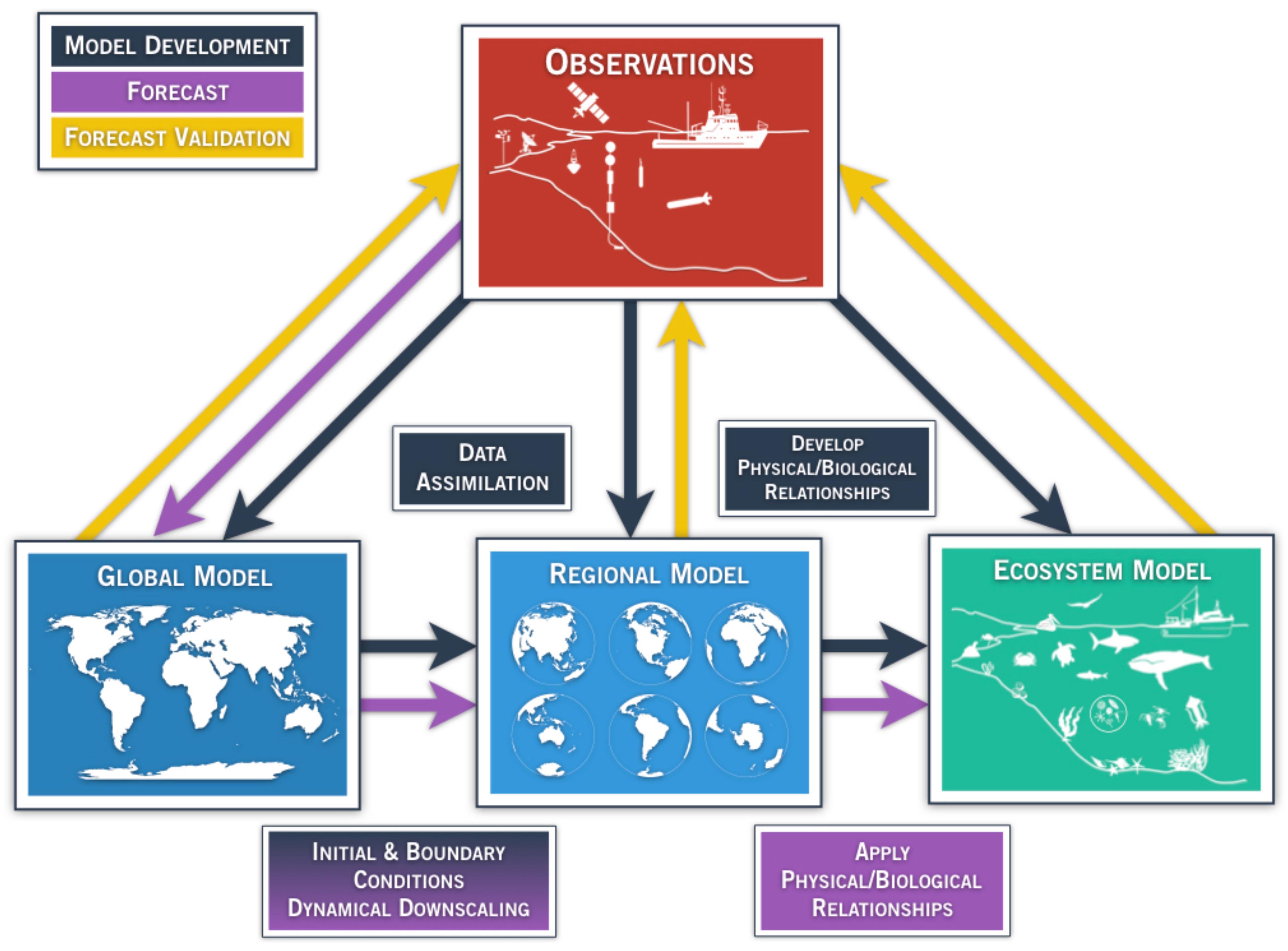
Figure 1. Generalized schematic of a physical-ecological forecast system. Arrows represent techniques for model development (black), ecosystem forecast/prediction (purple), and forecast validation (yellow). Global and regional models (blue boxes) assimilate available observing systems (red box) such as satellite data, tide gauge stations, drifting/moored buoys, profiling floats (e.g., ARGO), gliders, repeated trans-basin sections, regional ship time series, and radar observations. Observations also play a key role in the development of model parameterizations and statistical quantification among the components of the regional and ecosystem (green box) models, as indicated by the black arrow. Output from global models provide initial and boundary conditions for regional models (purple arrow), which dynamically extrapolate the effects of large-scale climate processes to regional or local scales of interest. The choice of the downscaling approach is part of model development (black arrow, shading from black to purple in the lower-left box). In addition, reliable and high-resolution operational observation systems are needed for validating, verifying, and determining the predictive skill of the forecast. Physical/biological relationships are developed based on historical observations (black box/arrow), and applied in the forecasting step. In the validation step, the output from the forecast system is compared with the appropriate observations (yellow arrows).

In the context of ecosystem-relevant predictions, the model can be a purely physical model at a global or regional scale (Figure 1, blue boxes), if the interest is primarily in the physical ecosystem drivers, or it can be online or offline coupled with an ecosystem model of various levels of complexity (Figure 1, green box). The online coupling strategy consists of running the physical and ecosystem models simultaneously whereas in the offline coupling, the ecosystem model is launched alone. In both strategies, the physical model provides the ecosystem model with the physical variables that are needed for the evolution of the biological quantities. For example, in a simple Nutrient-Phytoplankton-Zooplankton (NPZ) model, the biological variables will be advected by the model velocity field and diffused according to the physical diffusion coefficients (Franks, 2002). In addition, light and nutrient availability will be controlled by the physical model dynamics. In more complex models, however, light and nutrient availability are controlled by biological processes as well through, for example, phytoplankton absorption and bacterial re-mineralization (Skakala et al., 2018).

Both physical and biological models can either be empirical or dynamical. In the first case relationships among variables are determined from observations using statistical methods, while in the second case the prognostic equations linking the system variables at a given time to their values at a later time are solved numerically. For dynamical models, observations are needed to validate the model, to correct its parameterizations if needed, and identify missing processes (i.e., model development). In operational forecast systems, observations are also used to perform bias-corrections of the forecast in the presence of systematic model errors. The physical models considered in this paper are primarily high-resolution regional ocean models, for which the lateral ocean boundary conditions as well as surface forcing need to be provided. Initial and boundary conditions and surface forcing are obtained from global models, which are themselves constrained by observations through initial conditions and data assimilation.

Depending on the forecasting time scale τ, different observational inputs may be relatively more important. For forecasts up to several months, initial conditions are critical, but the memory of initial conditions is lost at longer lead times, so that boundary conditions and forcing become more important. In addition, observations are essential for validating the skill of the forecast, which includes assessing the reliability and quality of the forecast and refining or constraining forecast uncertainties.

In the following sections we provide examples of a variety of state-of-the-art statistical and dynamical forecasting activities focused on different regions along the North American coasts. These examples illustrate a broad range of approaches that exploit predictability associated with physical processes that are often specific to the different regions considered, and highlight observational needs for the different cases.

Statistical Forecasting Approaches

Linear Inverse Models

In the Linear Inverse Modeling (LIM) framework, the system of interest is described in terms of an anomaly state vector x, which is constructed from anomalies of the key system variables. The evolution of x is then modeled in terms of linearly damped and stochastically perturbed dynamics (Penland and Sardeshmukh, 1995; Newman et al., 2011) of the form:

$$d\mathbf{\text{x}}=\mathbf{\text{Lx}}dt+\mathbf{\text{Sr}}\sqrt{dt},(1)$$

where the matrix L encapsulates the predictable dynamics of the system, the matrix S represents the amplitude and spatial structure of the stochastic forcing, and r is a vector of random numbers drawn from a normal distribution with zero mean and unit standard deviation. Thus, the first term on the Right-Hand-Side (RHS) of equation (1) describes the changes of the state vector over the small time interval dt associated with deterministic processes, while the second term represents changes due to stochastic forcing as a random walk. The success of equation (1) in describing and predicting the system relies on the large time-scale separation between relatively slow oceanic processes and much faster non-linear atmospheric processes. These fast non-linear processes are represented by the stochastic forcing Sr $\sqrt{dt}$ in equation (1), and their systematic feedbacks on x, if any, are absorbed in L.

The L operator is estimated directly from the data as t_o^–1ln[C(t_o)C(0)^–1], where C(t_o) and C(0) are the covariance matrices of x at the training lag t_o (chosen to be 3 months) and at lag 0, respectively. Results are not sensitive to the choice of the training lag provided that the lag is sufficiently long that the noise can be treated as white noise, but shorter than intrinsic timescales of the system. Having determined L, the stochastic forcing amplitude S can be obtained from the Lyapunov equation:

$$\mathbf{\text{LC}}(0)+\mathbf{\text{C}}(0)\mathbf{\text{L}}{}^{\text{T}}+\mathbf{\text{SS}}{}^{\text{T}}=0.(2)$$

For a system described by (1) the most likely solution at time t + τ can be determined from the state at time t as:

$$\mathbf{\text{x}}(t+\mathrm{\tau })=\exp (\mathbf{\text{L}}\mathrm{\tau })\mathbf{\text{x}}(t)=\mathbf{\text{G}}(\mathrm{\tau })\mathbf{\text{x}}(t),(3)$$

where G(τ) = exp(Lτ). Equation (3) is used for forecasting applications. The LIM approach has been extensively used to model and predict SST anomalies in the tropical Pacific (Penland and Sardeshmukh, 1995; Newman and Sardeshmukh, 2017), but it has also shown skill for the prediction of SST anomalies along the U.S. west coast (Dias et al., 2018, Figure 2). For the latter application, the Hadley Center Sea Ice and Sea Surface Temperature (HadISST) data were used over the period 1900–2015. While a LIM constructed using only SST information has proven very useful in many applications, the inclusion in the state vector of information about subsurface ocean dynamics, for example thermocline depth or SSH has improved both modeling and prediction of the tropical Pacific system (Newman et al., 2011; Capotondi and Sardeshmukh, 2015; Capotondi and Sardeshmukh, 2017; Newman and Sardeshmukh, 2017), and may improve predictions in other regions. SSH is in itself a very important quantity to predict, given its dynamical link to thermocline depth, as well as its relevance for coastal sea level. The extension of the state vector to other variables (e.g., surface wind stress, ocean currents, sea surface salinity) may further improve the LIM system. An approach similar to the LIM has been successfully used to estimate the potential predictability of Net Primary Production (NPP) and SST over the global ocean, using satellite-based data of the two quantities over the period 1997–2017 (Taboada et al., 2019), although the short duration of the NPP record appeared to severely limit the skill of out-of-sample predictions of the last year of the data. Thus, future LIM applications can be expected to extend existing efforts to improve the modeling and forecasting of biological quantities.

FIGURE 2

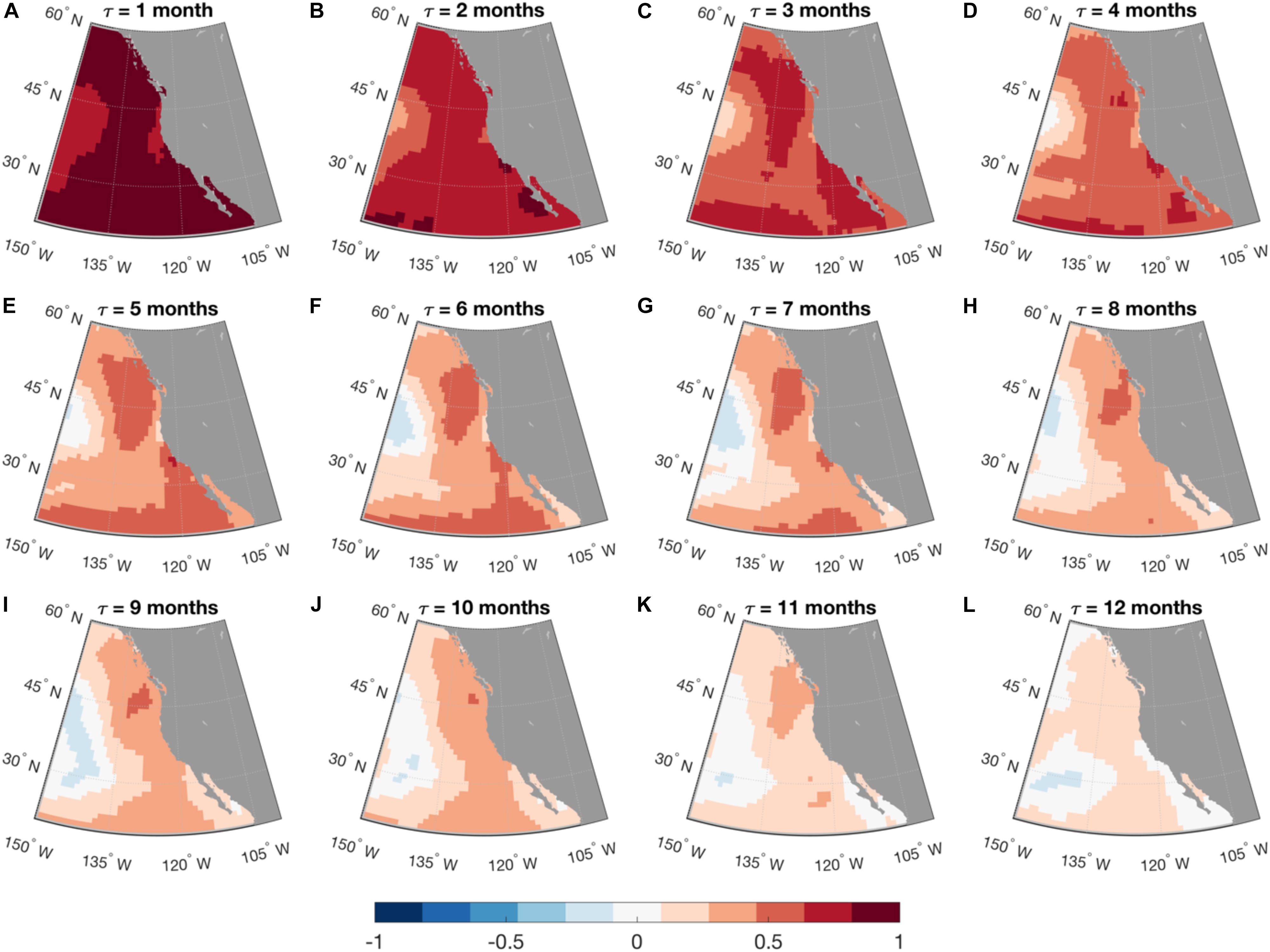
Figure 2. Linear Inverse Model forecasting. Maps of anomaly correlation coefficient (ACC) calculated between the forecasted and the observed SST anomalies in the Northeastern Pacific, as a function of lead time (t) from month-1 (A) to month-12 (L). Forecast was made using a linear inverse model (LIM) built with monthly SST anomalies in the North and Tropical Pacific. Forecast skill was cross-validated: LIM was trained using data from 1900 to 1994 and the forecast was made for the following 20 years, from 1995 to 2015.

The success of the LIM relies on the ability of the L and S operators, which are determined from the data, to capture the salient statistical features of the system of interest, which are themselves the expression of the system dynamics. Thus, long, accurate and consistent records of SST, SSH (or other measures of subsurface processes), surface atmospheric forcing (e.g., surface wind stress), and biological quantities are key to the robust determination of the LIM operators, and to the performance of this approach. While century-long SST data sets are now available (albeit with large uncertainties prior to ∼1950), the same is not true for SSH. The latter is usually obtained from reanalysis products, which themselves assimilate SSH observations from satellite altimetry after 1990. Thus, the continuation of the satellite missions providing large-scale SSH observations remains a high-priority for this type of applications. For predictions of SSH along the coast, accurate SSH data are needed for forecast verification. The availability of satellite data that are not contaminated by land, and have been carefully processed (e.g., for tidal removal), is high priority.

Synoptic Meteorology and Coastal Applications

In many studies of ocean-atmosphere interaction, multiple aspects of atmospheric forcing can play a role. An example is coastal sea level, for which atmospheric pressure, circulation, wind stress, storm surges, and wind-induced Ekman transport may all be important (Sweet et al., 2009; Sheridan et al., 2017). One method of analyzing the holistic influence of the atmosphere is through the use of synoptic climatology, more specifically, through atmospheric circulation-pattern identification. Each discrete atmospheric pattern over a region can then be related to an expected set of surface conditions, and their occurrence could be associated with anomalous marine events. Though there have been numerous different methodologies to classify atmospheric patterns, in recent years one method of classification has become increasingly used: self-organizing maps (SOMs; Sheridan and Lee, 2011), an artificial neural network-based classification technique in which circulation patterns are ordered in a two-dimensional continuum of patterns, with more similar patterns located in closer proximity than more dissimilar patterns. SOMs, generally used with regional fields of sea-level pressure, have been shown to be effective at examining the association between atmospheric circulation and coastal sea-levels (Sheridan et al., 2017), marine ecosystem structure (Kimmel et al., 2009), cold SST events and thermal stress in marine species (Pirhalla et al., 2015), water clarity (Pirhalla et al., 2016), and chlorophyll levels (Sheridan et al., 2013).

Using the synoptic methodology has some limitations, such as that it will not fully capture the most extreme atmospheric events (e.g., hurricanes), due to their atmospheric circulations being effectively ‘unique’ and thus hard to generalize. However, the categorization of the atmosphere into patterns yields substantive statistical power to assess the correlation between the atmosphere and ocean properties. Further, the synoptic methodology serves as an effective statistical downscaling tool for output from weather-forecasting or global-climate models (Schoof, 2013), which in some cases has proven to be superior to finer-scale model-generated atmospheric data (Wetterhall et al., 2009).

The success of this approach relies on the availability of atmospheric and oceanic fields at sufficient temporal and spatial resolution to capture the small-scale variations of interest at synoptic timescales, and of adequate duration to establish reliable statistical relationships between atmospheric and oceanic variables. For example, the analysis of thermal stress of marine species in the western Florida shelf by Pirhalla et al. (2015) utilized a suite of satellite-based SST products at 9km horizontal resolution covering the period 1982–2012. Similarly, an ongoing study on the influence of weather and climate on biodiversity in the Channel Islands National Marine Sanctuary, CA, uses data at moderate-scale (4km) resolution to analyze cross-shelf SST gradients as a proxy for coastal upwelling (unpublished data).

Global Dynamical Models

Global models, including coupled climate and Earth system models, can capture the dynamic, non-linear interactions of Earth system components and how those interactions express as variability and change in various simulated physical and ecological systems. Relevant to marine ecosystem simulation, Earth System Models are increasingly integrating biogeochemical descriptions and routines that dynamically interact with the physical systems simulated by the model (Dunne et al., 2013; Hurrel et al., 2013). This model development work increases the relevance of Earth system models for investigating and simulating ecosystem behavior and potentially predicting it.

Because of their ability to represent dynamic physical behavior and system interactions, global models capture modes of variability observed in the climate system as well as projections of those modes onto components of the Earth system, offering predictability on a variety of timescales. For marine ecosystem prediction, the ability of models to accurately forecast physical ecosystem drivers like currents and water temperatures provides foundational information that can be used to understand ecosystem health and expected behavior, especially for target species that are strongly driven by physical environmental factors.

Global climate and Earth system models are routinely used for seasonal prediction at operational prediction centers around the world. Applications of these seasonal prediction systems are diverse, and marine ecosystem prediction efforts have just begun to harness global dynamical seasonal prediction systems for skill. Early efforts in the U.S. have harnessed output from the North American Multi-Model Ensemble (NMME, Kirtman et al., 2014), which includes seven research and operational models from five research and operational centers run in real time on a monthly schedule. The NMME provides a large multi-model ensemble dataset to evaluate and forecast climate variability on seasonal to interannual timescales.

NMME model data is provided at a relatively coarse 1°×1° resolution, but is useful for capturing large-scale oceanic variability and drivers of that variability that offer predictability. The NMME’s ability to capture relevant modes of variability has been well-documented (Becker et al., 2014; L’Heureux et al., 2017) and the consistent set of hindcasts offers the opportunity to evaluate the applicability of the system for targeted predictions. In particular, the NMME model output can supply lateral boundary conditions and surface forcing, after proper downscaling, for high-resolution regional forecasting models like those described in Sections “JISAO’s Seasonal Coastal Ocean Prediction of the Ecosystem (J-SCOPE)” and “Bering Sea Modeling and Forecasting.” Only information of physical quantities is provided at present by the NMME system.

An example of a high-resolution, global coupled ocean-biogeochemical model used for operational physical and biogeochemical forecast is the Mercator Ocean Model³. The Mercator system uses the Nucleus for European Modelling of the Ocean (NEMO) ocean model⁴ at 1/12° horizontal resolution coupled with a biogeochemical model at 1/4° resolution. Many different data sources are assimilated in the model, including, in particular, real time along track sea level anomalies from AVISO⁵, SST from both remote sensing [e.g., the Operational Sea Surface Temperature and Sea Ice Analysis (OSTIA) at daily time resolution, Donlon et al., 2011] and in situ sources, and temperature/salinity profiles from Argo floats. Mercator ocean provides daily forecasts of physical variables and weekly global biogeochemical forecasts. In particular, daily environmental conditions in support of the Tara expedition (section Toward Holistic Marine Ecosystems Monitoring for Improving Ocean Models) were obtained from the real-time output of the Mercator Ocean.

Global Earth System Models of sufficiently high horizontal resolution to realistically capture small-scale ocean circulation features (e.g., eddies and filaments) and their response to climate variations provide invaluable tools for studying physical and biogeochemical coastal processes by seamlessly connecting the small-scale coastal dynamics to the large scale oceanic and atmospheric circulations. However, the initialization and spin-up of global climate models that include biogeochemistry is challenging. Due to the large number of variables in the biogeochemical model relative to the physical model component the spin-up of the model biogeochemistry may require thousands of years (Wunsch and Heimbach, 2008) compared to weeks for the atmosphere and centuries for the ocean and ice components (Stouffer et al., 2004). Also, biogeochemical data are very sparse. Three-dimensional climatology datasets available for biogeochemical initialization exist only for few variables (macro-nutrients, oxygen, dissolved carbon and alkalinity) while data are extremely sparse for other variables, including dissolved organic carbon, dissolved iron, as well as the biomass of various plankton types. As a result, the latter fields are often initialized as constant fields, producing a mismatch with the physical ocean state, and leading to incomplete equilibration in coupled simulations (Seferian et al., 2016). While in regional model configurations empirical algorithms can be used to relate the physical data (e.g., temperature and salinity) to the biogeochemical variables of interest locally (Siedlecki et al., 2015) these empirical relationships may not be applicable at the global scale. Thus, the global expansion of BG-Argo floats would be extremely valuable for providing measurements of biogeochemical quantities to be used for biogeochemical data assimilation and model initialization.

Regional Applications

The U.S. West Coast

Along the U.S. West Coast upwelling is a major driver of ecosystem variability at all timescales. Nutrients upwelled to the sunlit surface layer stimulate blooms of phytoplankton that provide the energy base for the marine food web. Consequently, variability in upwelling intensity and the nutrient content of upwelled waters controls primary production in the California Current System (CCS) (Jacox et al., 2016). On interannual timescales, the timing and amplitude of the seasonal cycle (phenology) has been shown to have a large impact on ecosystem functioning. The peak upwelling season in the CCS typically occurs during April-July (Garcia-Reyes and Largier, 2012), with disruptions in phenology leading to dramatic changes in ecosystem composition and abundance (e.g., Schwing et al., 2006). In addition to supplying nutrients to the nearshore region, upwelling can also bring low oxygen, corrosive waters to the continental shelf (Feely et al., 2008, 2016; Chan et al., 2017). ENSO and the PDO modulate upwelling at interannual and decadal timescales, respectively, with the former providing a source of seasonal predictability. Downwelling equatorial Kelvin waves that propagate eastward during the development of an El Niño event continue poleward along the western coasts of the Americas as coastally trapped waves, where they deepen the thermocline and contribute to reduced upwelling in those areas, thus providing an oceanic pathway for the ENSO influence on ocean conditions along the west coast of the Americas. In addition, tropical convection associated with equatorial SST anomalies excites atmospheric teleconnections that alter mid-latitude atmospheric circulation, resulting in upwelling that is anomalously weak (strong) during El Niño (La Niña) events. This atmospheric response to ENSO variability is a source of seasonal predictability in the CCS (Jacox et al., 2017), and has important consequences for primary production, fish abundance and species distribution (e.g., Chavez et al., 2002 and references therein). It is important to note that the winds that drive this upwelling have intensified over recent decades, driving the increased presence of corrosive conditions in the CCS (Turi et al., 2016), though future trends in upwelling intensity are likely to be dependent on latitude and season (Rykaczewski et al., 2015). Given the uncertain future of coastal upwelling variability and change, and its impact on the physical, chemical, and biological state of the CCS, it is clear that sustained ocean monitoring of this region is critical.

Oxygen modeling of the Washington and Oregon shelves

Regional models have developed to the point of being able to address process based questions and be compared to observations at high spatial and temporal resolution. For example, modeling work has identified processes that control the spatial variability and timing of hypoxic ocean conditions on Washington and Oregon shelves (Siedlecki et al., 2015). Regions of persistent hypoxia correlated with regions of high respiration in the region, and corresponded to regions previously identified as retentive or recirculation regions. These results were limited to simulations of 2005–2007, but the locations that persistently experienced hypoxia are also present in the climatology of summer conditions from the JISAO’s Seasonal Coastal Ocean Prediction of the Ecosystem (J-SCOPE) simulations spanning 2009–2017, and consistent with recent observations in those regions. The attribution of the respiration process to spatial and temporal variability of hypoxia relied on many levels of observations including subsurface mooring time series, observations of sediment oxygen demand at the sediment-water interface, and benefited from regional observations of rates for some key ecosystem processes (e.g., respiration, sinking, sediment oxygen demand, zooplankton grazing).

JISAO’s seasonal coastal ocean prediction of the ecosystem (J-SCOPE)

The J-SCOPE model⁶ features dynamical downscaling of regional ocean conditions in Washington and Oregon waters using a combination of a high-resolution regional model with biogeochemistry and forecasts from NOAA’s Climate Forecast System (CFS). The regional model (ROMS) extends from 43°N to 50°N with a horizontal resolution of 1.5 km and 40 vertical levels. The CFS fields are interpolated to the regional model grid, and used for lateral boundary conditions of the physical fields, surface forcing and initialization. Lateral boundary conditions of the biogeochemical fields use empirical relationships that relate these fields to salinity. The forecast experiments of J-SCOPE experienced significant biases inherited from some of the CFS variables, highlighting the importance of the global models forecast skill for the performance of the regional forecasting system.

The J-SCOPE forecasts are developed to support the California Current Integrated Ecosystem Assessment. Integrated Ecosystem Assessments (IEAs) are a framework for informing ecosystem-based management, which aims to account for interactions among ecosystem components and managed sectors, as well as cumulative impacts of a wide spectrum of ocean-use sectors (Levin et al., 2009). In the context of the California Current IEA, J-SCOPE provides 6- to 9-month forecasts of ocean conditions that are testable against observations and relevant to management decisions for fisheries, protected species, and ecosystem health. Results will directly inform the IEA process and will forecast indicators requested by the Pacific Fishery Management Council.

Experiments suggest that seasonal forecasting of ocean conditions important for fisheries is possible with the right combination of components, with forecast uncertainty dependent on the variables and specific region of interest. The components that have proved to be critical for the success of the J-SCOPE system include regional predictability on seasonal timescales of the physical environment from a large-scale model, a high-resolution regional model with biogeochemistry that accurately simulates seasonal conditions in hindcast mode (short simulations that incorporate data assimilation), a relationship with local stakeholders, and a real-time observational network, a result that is consistent with an emerging body of literature (Hobday et al., 2016; Tommasi et al., 2017).

J-SCOPE has considerably benefited from the availability of data from an in situ cruise during 2009–2014, as well as bi-weekly measurements of physical and biogeochemical quantities at three moorings located within the model domain. Figure 3 showcases all the observations that have been used to evaluate the model. This has allowed validating both the physical and biogeochemical model components, as well as the model forecasts. In particular, J-SCOPE model performance and predictability were examined for SST, bottom temperature, bottom oxygen, pH, and aragonite saturation state through model hindcasts, forecast (forcing without data assimilation), and re-forecast (forecasts performed on past years) comparisons with observations. Results indicate J-SCOPE forecasts have measurable skill on seasonal timescales (Kaplan et al., 2016; Siedlecki et al., 2016). Bottom ocean conditions (e.g., bottom temperature and bottom oxygen), which are very important for benthic dwelling species, like Dungeness crab, were shown to have more predictability than SST in this region (Siedlecki et al., 2016).

FIGURE 3

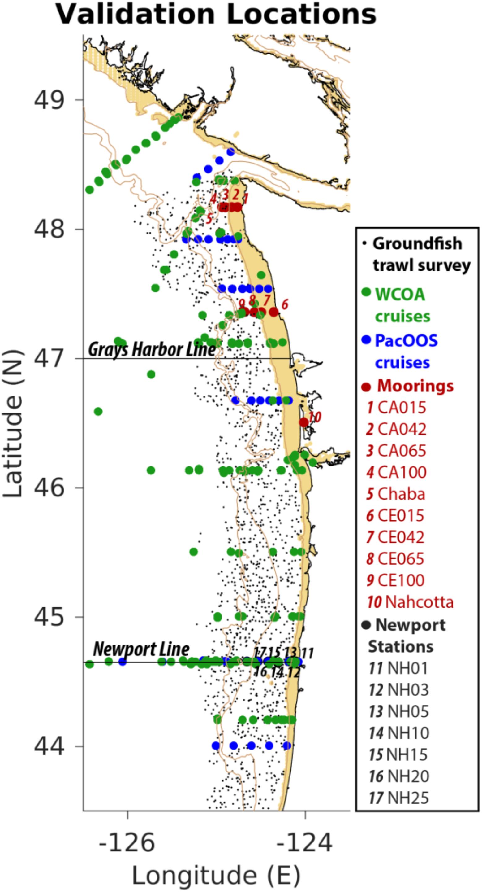
Figure 3. Mixed data sources contribute to model initialization and evaluation – J-SCOPE. The J-SCOPE model depends on a series of data sets to continually evaluate the model’s skill. In addition, some of the data sets contribute to regional algorithms that allow the physical data (salinity and temperature) to be extended to oxygen and carbon variables. The data depicted cover different time periods and monitor different suites of variables spanning 2009–2017. The NOAA West Coast Ocean Acidification Cruises (WCOA) are performed every fourth year in the summer upwelling season and provide extensive biogeochemical as well as biological observations in the region. Occupation of the Newport stations, sponsored by NOAA, occurs bi-weekly year-round, and include nutrient, oxygen, biological, and temperature observations, and occasionally inorganic carbon. The ground fish trawl survey is performed every year by the NOAA Northwest Fisheries Science Center and measures temperature as well as oxygen near the bottom. The moored observations in red are composed mainly of moorings located within NOAA’s Olympic Coast National Marine Sanctuary (OCNMS) that are deployed seasonally. These monitor temperature at the surface and at depth and oxygen at depth. The Chaba mooring (mooring #5), sponsored by the Northwest Association of Networked Ocean Observing Systems (NANOOS), and maintained by the University of Washington, measures temperature, salinity, oxygen, fluorescence, and velocities over the water column and pH at depth; through collaboration with NOAA PMEL, it also monitors carbon dioxide and pH at the surface. The full CCS-wide list of data relevant to ocean acidification and hypoxia is detailed in Chan et al. (2016).

Observations are critical to the development and testing of systems like J-SCOPE. J-SCOPE depends on them in three primary ways: (1) model development and performance evaluation; (2) for constraining initialization and boundary conditions, and (3) for engendering trust with stakeholders and end users through forecast evaluation and uncertainty communication efforts. These observations include regional rate estimates on the lower trophic level ecosystem cycling described in Banas et al. (2009) and Davis et al. (2014), time series from moorings including those operated by NOAA and the OCNMS (Giddings et al., 2014; Siedlecki et al., 2015, 2016), satellite products of SST, SSH and Chlorophyll (Davis et al., 2014; Giddings et al., 2014), observations taken as part of groundfish surveys performed by NOAA, and water column observations of chemistry performed every few years by NOAA’s OAP and regional projects like PacOOS or the WOAC.

Assessing the physical-biogeochemical response of the California Current System (CCS) to ENSO

While high-resolution regional modeling is an excellent approach to achieve a detailed representation of the physical and biogeochemical coastal processes in the region of interest, it does rely on the availability of lateral boundary conditions and surface forcing fields that are usually provided by global models, and are therefore impacted by those global model biases. The prescription of lateral boundary conditions from global models is especially limiting in regions that are influenced by inflows of remote origin. The CCS is an obvious example. Coastal Kelvin waves excited along the equator during ENSO events enter the domain from the southern boundary of the CCS region, and can produce important modulations of the pycnocline depth in the region. Thus, prescription of biased lateral boundary conditions to a regional CCS model may distort these important influences. In this application, a global high-resolution physical biogeochemical model with a realistic representation of the small-scale features of the CCS was used to assess the response of ocean pH and oxygen, important ecosystem stressors, to ENSO events (Turi et al., 2018).

Findings from this study draw attention to the following:

(1) The manifestation of ENSO events in the CCS shows large variations from event to event. While this diversity can be partly attributed to the diversity of ENSO events in the equatorial Pacific (Capotondi et al., 2015), and the large spread in the atmospheric response to equatorial SST anomalies (Sardeshmukh et al., 2000), due to atmospheric noise, these event-to-event differences do highlight the need for sustained observations of physical and biogeochemical quantities to monitor the diversity of ENSO influences on the CCS, in the presence of low-frequency natural variability and climate change.

(2) Biogeochemical properties in the surface ocean may respond differently to ENSO than the same properties at depth. For example, as shown in Figure 4, during El Niño events oxygen decreases at the surface, but increases at depth in a narrow band along the coast, while pH shows a similar behavior both at the surface and at depth. Thus, observations spanning the full depth of the water column in this region, and capable of resolving the narrow high variance region along the coast are required to understand the response of these variables to ENSO.

(3) In spite of the extensive observational network in the CCS regions, some biogeochemical data are either not available or sparse, or of insufficient duration to allow the validation of this high-resolution model simulation in this region in a climatological sense. Water column measurements of Dissolved Inorganic Carbon (DIC) and Alkalinity (Alk), which are needed to calculate pH, CO₃, and aragonite saturation, are not regularly measured except from a few locations within the CCS. Surface measurements of pCO₂, which are critical for estimating CO₂ flux and validating model solutions, are very sparse. Indeed, Figure 5 shows that there are fewer than 3,000 shipboard observations of surface ocean pCO₂ over the CCS region during 1982-present. This is a coverage similar to that of the data-poor Southern Ocean region. Finally, water column measurements of O₂, which are measured at CalCOFI, are sparse in large areas of the ocean.

FIGURE 4

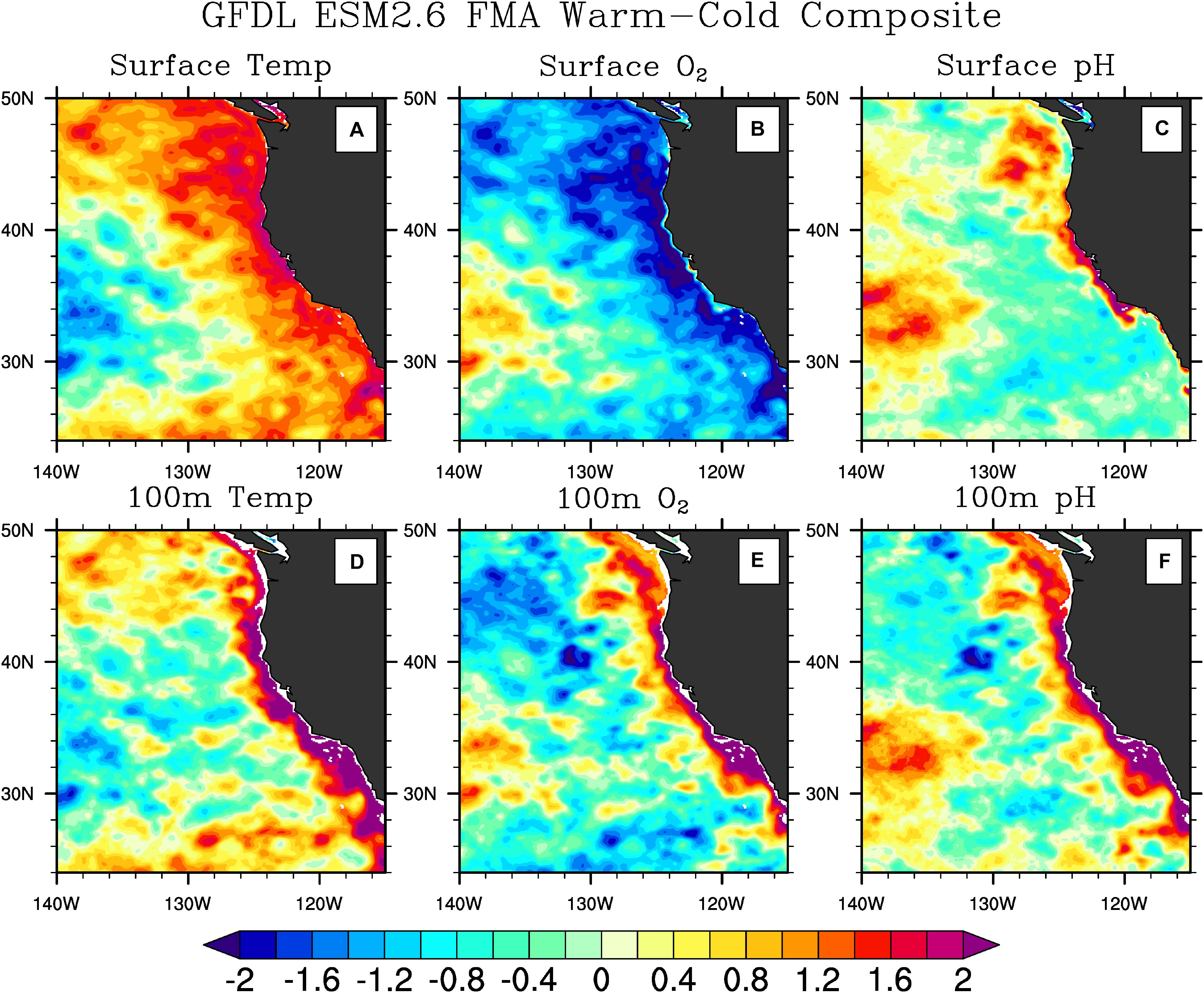
Figure 4. ENSO influence on the CCS in a high-resolution global physical-ecosystem model. Composites (warm minus cold) of temperature (A,D) (left panels), O2 (B,E) (middle panels), and pH (C,F) (right panels) at the surface (A–C) (top panels) and at 100 m depth (D–F) (bottom panels) of 6 El Nino and 7 La Nina events during February–March–April from the Geophysical Fluid Dynamics Laboratory (GFDL) Earth System Model version 2.6 (ESM2.6). The composites were computed by averaging each quantity at each model grid point over the 6 El Niño events detected in the 52-year model simulation, and then subtracting the average of the same quantities during the 7 La Niña events present in the simulation. The “warm minus cold” approach was used to increase the signal-to-noise ratio. The model resolution is 0.1°. Anomalies are standardized by dividing the time series at each grid point by their interannual standard deviation. Notice the difference in the horizontal and vertical spatial structures of different quantities. Temperature and O₂ anomalies have a broader structure at the surface than at pycnocline depth, while pH anomalies are concentrated near the coast at both depths. Notice how O₂ anomalies have a different sign at the surface and at depth. These differences in spatial structures suggest the need for monitoring at different depths in the water column to capture property changes. The figure was modified from Turi et al. (2018) under the Creative Commons Attribution 4.0 License.

FIGURE 5

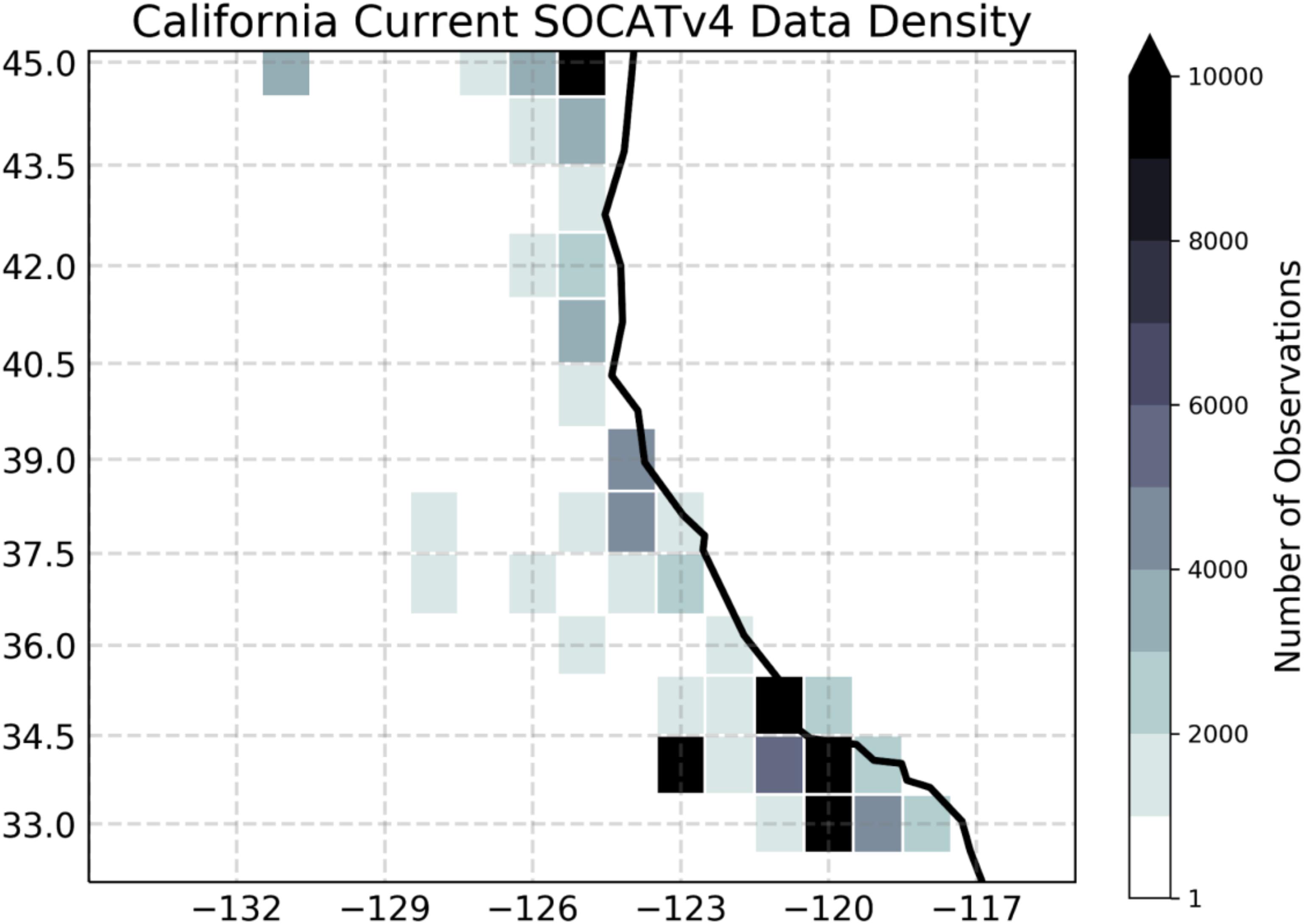
Figure 5. Density of in situ observations for the surface ocean partial pressure of carbon dioxide. Shading shows the total number of shipboard measurements in each 1 × 1 degree grid cell between 1982 and 2015, based on the SOCATv4 data set (Bakker et al., 2016). The figure was modified from Brady et al. (2018) under the Creative Commons Attribution 4.0 License.

These observational needs are also critical for initializing forecasts in this and other coastal regions.

The Northwest Atlantic

Variability in ocean temperature in the Northwest Atlantic, and in particular in the northeast shelf (NES) is directly linked to two dominant processes: air-sea heat flux, primarily operating on scales of days to months, and ocean advection, operating on scales of months to years. Recent studies demonstrated that an extreme Northeast U.S. warming event observed in 2012 was primarily driven by anomalous wintertime air-sea heat flux, with smaller contributions from ocean advection. However, the relative influence of air-sea heat flux and ocean advection varies from year-to-year (Chen et al., 2014, 2015, 2016). The air-sea heat flux is significantly correlated with the latitude of the atmospheric jet stream, especially in winter and autumn.

Located at the downstream end of an extensive coastal boundary current system, the NES is the direct recipient of cold and fresh water of Arctic origin through accumulated coastal discharge and ice melt that has been advected thousands of kilometers around the boundary of the subpolar North Atlantic. Likewise, subtropical water masses, advected by the Gulf Stream, slope currents, and associated eddies, also influence the composition of water masses within the NES region. The relative strength of the Labrador slope water and warm slope water adjacent to the Gulf Stream have been shown to affect salinity, nutrients, and temperature on the shelf, as well as zooplankton assemblages and upper trophic level productivity (Green et al., 2013). One of the best leading indicators of the interplay of these two current systems is the latitude of the Gulf Stream (GS) path. Indeed, in situ measurements suggest a direct link between the GS position and the temperature and salinity near the shelf break south of New England (Gawarkiewicz et al., 2012).

Modeling the Northwest Atlantic

The Northwest Atlantic is a highly complex system that sits at the interface of two major current systems, the Gulf Stream and Labrador Current. Both of these currents highly influence the oceanography of the region as does its complex bathymetry such as the Grand Banks, Georges Bank, and Browns Bank. Therefore, ocean models need to resolve both the regional ocean circulation and complex bathymetry of the region in order to forecast near-term or projected long-term ocean conditions (Figure 6).

FIGURE 6

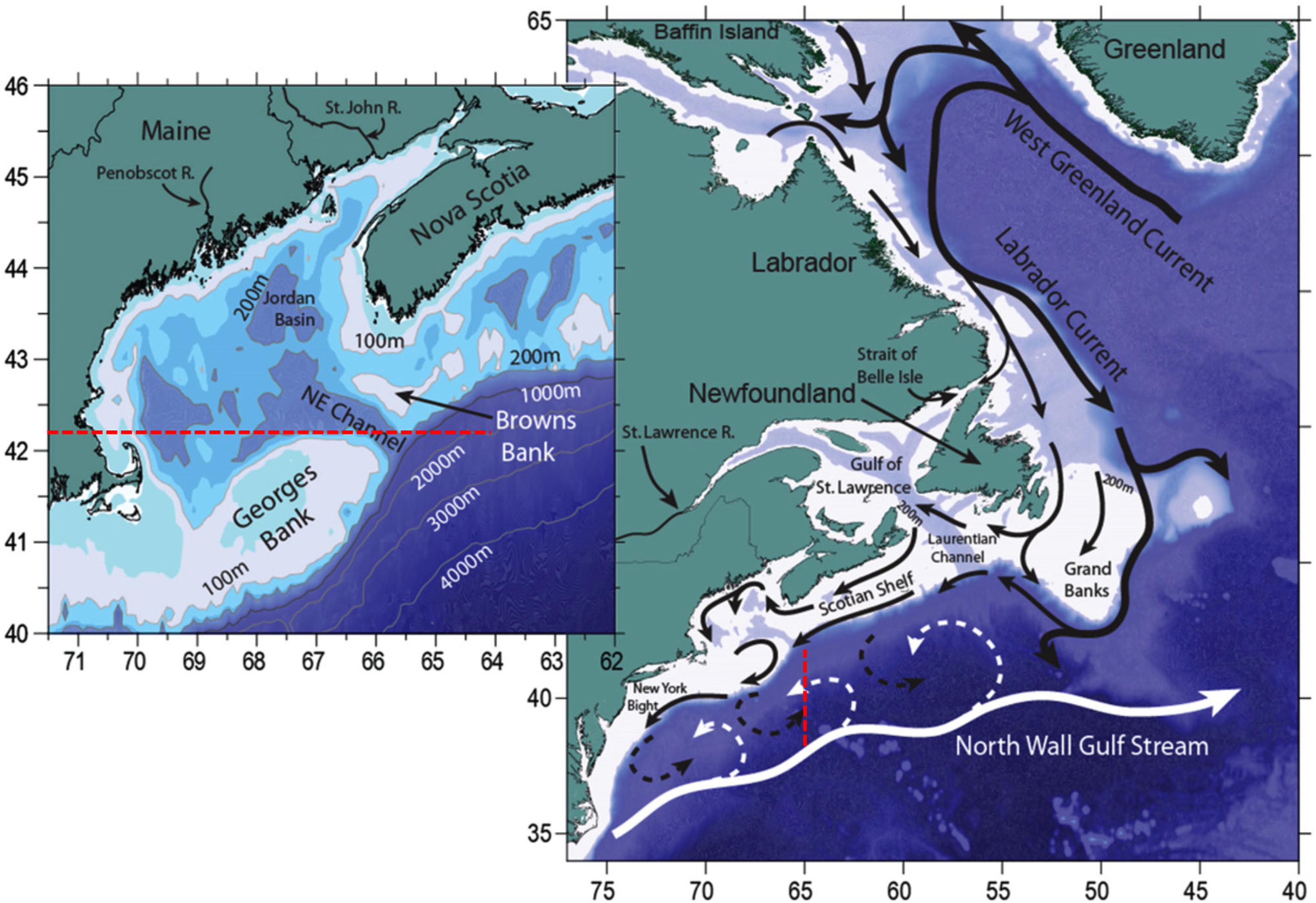
Figure 6. Northwest Atlantic Ocean and Labrador Sea bathymetry and major currents. Black arrows indicate colder and fresher water from the Labrador Current, while the white arrows indicate warmer and saltier Slope waters of Gulf Stream origin. Dashed arrows indicate areas where mixing can occur. The inset shows the location of the Northeast Channel (NE Channel) where a mixture of Labrador Current waters and Slope waters enter the Gulf of Maine. The figure was reproduced from Saba et al. (2016) with permission from AGU.

Both regional and global models have been commonly used to study the physics and biogeochemistry of the Northwest Atlantic. Regional models include ROMS and the Finite Volume Community Ocean Model (FVCOM), both of which have physics-only simulations as well as simulations coupled with biogeochemical models. These regional ocean models are typically forced by reanalysis data at their ocean boundaries and at their ocean-atmosphere interface, and therefore may suffer from the biases of the forcing fields. Also, as reanalysis data have typically coarser resolutions, they may miss smaller scale features entering the high-resolution model domain. Global climate models participating in the Intergovernmental Panel for Climate Change (IPCC) fourth and fifth assessment reports have also been used to study the oceanography and climate of this region although they are generally limited by their coarse horizontal spatial resolution (∼100 km) in their ocean component. These global models exhibit a persistent bias in the coastal separation point of the Gulf Stream such that the current overshoots and separates from the U.S. east coast too far to the north, leading to very large positive SST bias to the north of the observed Gulf Stream position. However, a prototype high-resolution (∼10 km ocean resolution) global climate model (CM2.6) developed by NOAA’s Geophysical Fluid Dynamics Laboratory (GFDL) shows a reduced bias in the Gulf Stream separation, and is able to resolve the regional circulation and bathymetry of the Northwest Atlantic (Saba et al., 2016). This high-resolution climate model is not a forecasting model but was used to examine the projected changes in the Northwest Atlantic associated with a 1% per year increase in atmospheric CO₂ over a 70-year period. Results indicate large temperature increases in the region associated with the CO₂ increase, which were not obtained with other GFDL models run at coarser resolutions. Thus, this model has provided very important insights on climate change in the Northwest Atlantic (Saba et al., 2016). Temperature and salinity measurements in the Gulf of Maine Northeast channel, the major throughway for Slope Waters to enter the shelf at depth (Mountain, 2012) have allowed the model validation at the fine scale of the Channel. This modeling activity has also largely benefited from relatively high-resolution (0.25°) NOAA Optimum Interpolation SST (OISST) data (Reynolds et al., 2007) over a long enough period (1981–2013) to allow the establishment of a reliable SST climatology at the spatial scales relevant for this high-resolution model. Bottom temperature and salinity data from the NOAA Northeast Fisheries Science Center’s fall and spring bottom trawl survey and ecosystem monitoring survey also provided critical in situ ocean data to estimate model biases.

Temperature predictions in the Northwest Atlantic

The Northwest Atlantic is arguably one of the most dynamic systems in which to explore predictability. In addition to being a temperate system with high seasonality, the coupled Slope Water system causes isotherms to be very close together and their location changes annually due to large-scale oceanographic and atmospheric processes. Because of this spatially and temporally dynamic environment, SST along the Northeast U.S. coast has been shown to have low predictability especially at long time scales (Stock et al., 2015). However, other analyses that have considered subsurface variables indicate the existence of larger predictability in this region. Chen et al. (2016) estimate that the depth-integrated temperature over the NES during winter-spring has a mean decorrelation time scale of ∼50 days, with decorrelation timescales much longer near the bottom than at the sea surface. This mean decorrelation time scale indicates the possibility of some seasonal predictability, and the lead time for skillful predictions may increase when a multivariate system is considered.

As described above, well-established relationships exist between climate aspects of this coupled slopewater system and the local physical quantities that are directly related to the distribution and abundance of zooplankton and fish. Oceanographic features that show some predictability and that relate to ecological endpoints include the Gulf Stream path (Joyce et al., 2000; Nye et al., 2011), coastal sea level (Forsyth et al., 2015), local along-shore wind (Li et al., 2014), atmospheric jet stream latitudes at various longitudes (Chen et al., 2014), PDO (Pershing et al., 2015), and NAO (Joyce et al., 2000; Frankignoul et al., 2001).

Activities are underway to relate the temperature in the NES region to various predictands (e.g., Gulf Stream path, along-shore wind etc.) through multiple linear regressions. The skill of this statistical model must be evaluated using observations and/or hindcast and reanalysis products. The determination of the statistical model coefficients, as well as the model validation, require long time series of both predictands and predictors to allow the establishment of statistically significant relationships.

Bering Sea Modeling and Forecasting

In subarctic regions like the Bering Sea, sea ice and bottom temperature are major drivers and determinants of ecosystem state, with the timing and extent of sea ice cover and open waters influencing the evolution of the seasonal cycle in the region. Date of ice retreat, combined with solar heating and wind mixing determine the timing of the spring bloom on the southern Bering Sea shelf, with early ice retreat favoring late blooms in May or June, and late ice retreat (after March) favoring early phytoplankton blooms (Stabeno et al., 2007). Warm and cold years, as defined by water temperatures between the surface and 70 m depth, correlate to low and high abundance of large zooplankton in the southeastern Bering Sea shelf (Coyle et al., 2011), and the “cold pool,” the area where the bottom temperature is less than 2°C, has been found to influence the distribution of major commercial groundfish (Lauth and Kotwicki, 2013). The southern edge of the cold pool itself has shifted ∼230 km north since the early 1980’s (Mueter and Litzow, 2008).

The importance of the Bering Sea region for commercially valuable fish species has stimulated extensive high-resolution modeling efforts in this region. The regional model (named “Bering10k-ROMS”) is based on the Regional Ocean Modeling System (ROMS, Haidvogel et al., 2008) with ∼10 km horizontal resolution and 10 vertical layers. The model domain extends from the western Gulf of Alaska to the Russian coast and to slightly north of the Bering Strait (Figure 7). It is coupled to an ice model and to a lower trophic level NPZ model (known as BESTNPZ, Gibson and Spitz, 2011) with ice-related dynamics and two-way interactions: Bering10k-ROMS feeds ocean currents, temperature and sea ice cover to the NPZ model, which in turn provides phytoplankton density, a quantity that affects attenuation of shortwave radiation and thus heat absorption in the upper water column (Hermann et al., 2013, 2016). The BESTNPZ-Bering 10k-ROMS is additionally coupled to a fish model, the Forage and Euphausiid Abundance in Space and Time (FEAST), which is a 2-dimensional, gridded, daily scaled multispecies length-based foraging, bioenergetics movement and recruitment model for post larval forage and predatory fish (Ortiz et al., 2016). Together, these models form the Bering10K Modeling Suite (hereafter Bering10K), and were originally designed under the supervision of an ecosystem modeling committee as part of an integrated ecosystem research program, “The Bering Sea Project⁷,” to synthesize up-to-date information about the eastern Bering Sea ecosystem and be used both for research and management purposes (Punt et al., 2016). An ocean acidification module has recently been added to the Bering10K modeling suite. For seasonal forecasting using the Bering10K, lateral boundary conditions and surface forcing are provided by the NOAA CFS model.

FIGURE 7

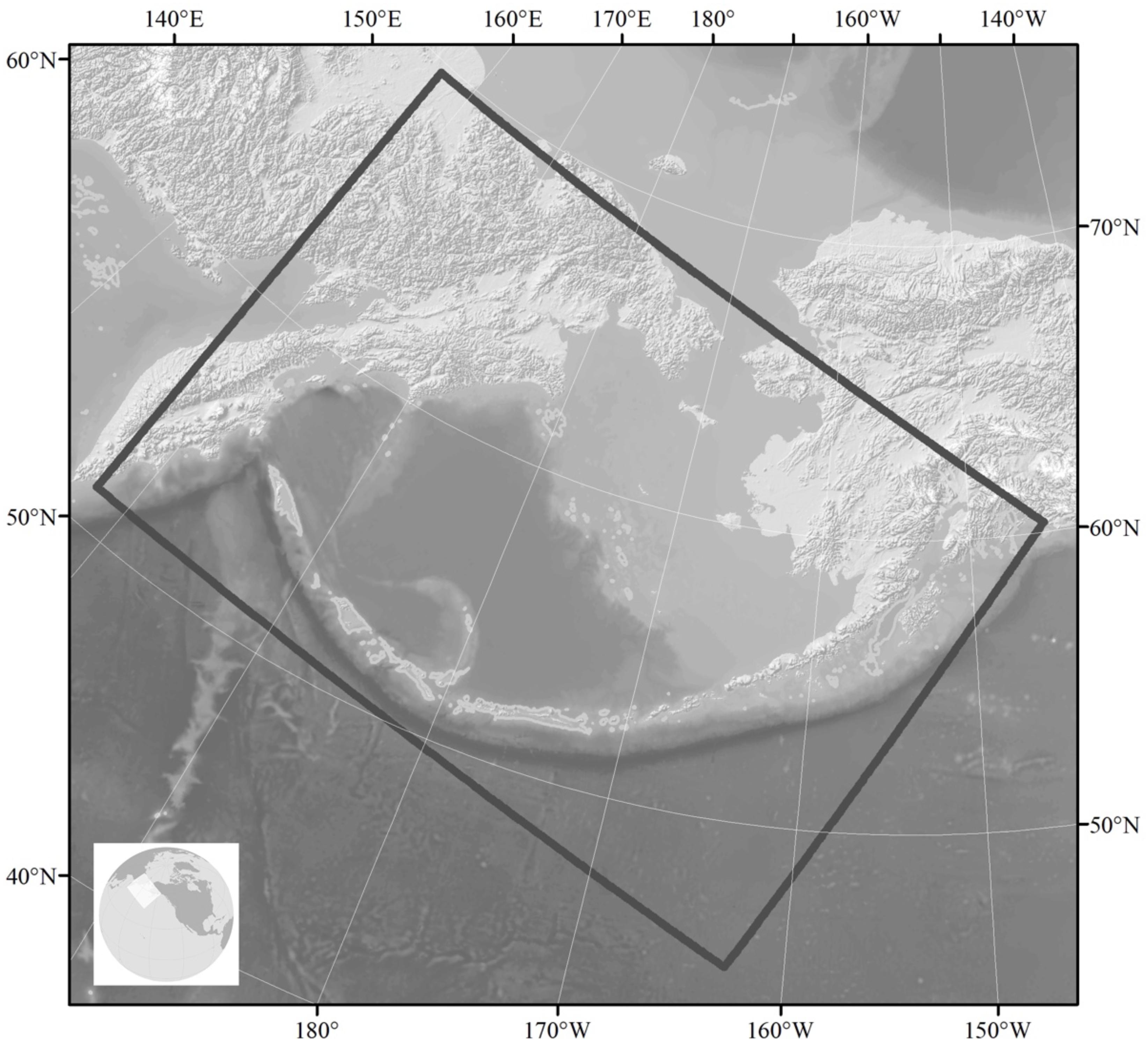
Figure 7. Geographical extent of the Bering10K Modeling Suite showing bathymetry. The primary focus is on the eastern Bering Sea shelf, where in cold years sea ice cover can extend from the Bering Strait to the Alaska Peninsula and retreat in the SE as late as the end of April. The influence of sea ice persists through summer, as cold, dense salty water remains in the bottom as a “cold pool” that typically persists along the middle shelf south of 58°N.

The Bering10K plays a key role within the region’s work on IEAs⁸, ecosystem-based fisheries management and strategic planning, and is at the core of the Alaska Regional Climate Action Plan for the Southeastern Bering Sea (Sigler et al., 2016). The output from Bering10K is used in multiple operational/testing products (see Figure 8). In particular, Bering10K-ROMS-BESTNPZ driven by CFS global output has provided a 9-month forecast of the cold pool for the past 5 years; the forecast is included in the annual Bering Sea Ecosystem Considerations Chapter and presented annually to the North Pacific Fisheries Management Council. Bering10k_ROMS has been used to produce ensemble climate projections to the end of the 21st century, using selected global models from the Coupled Model Intercomparison Projects phase 3 and phase 5 (CMIP3, CMIP5) for initial and boundary conditions and surface forcing. The results showed a significant decrease and northward shift of the cold pool (Hermann et al., 2016). The dynamically downscaled temperature from the hindcast and projection simulations, with both CMIP3 and CMIP5 forcing, has been used to evaluate future essential fish habitat (EFH) and ecosystem indicators under different emission scenarios. Both temperature and zooplankton are used in several models that are part of the Alaska Climate Integrated Modeling Project. The Bering10K is also being used to inform the Climate Action Module for the Bering Sea Fisheries Ecosystem Plan, currently under development by the NPFMC⁹. Finally, hindcast of walleye pollock distribution and abundance and forecasts from FEAST will be used as part of a project evaluating the effects of climate change on northern fur seals¹⁰.

FIGURE 8

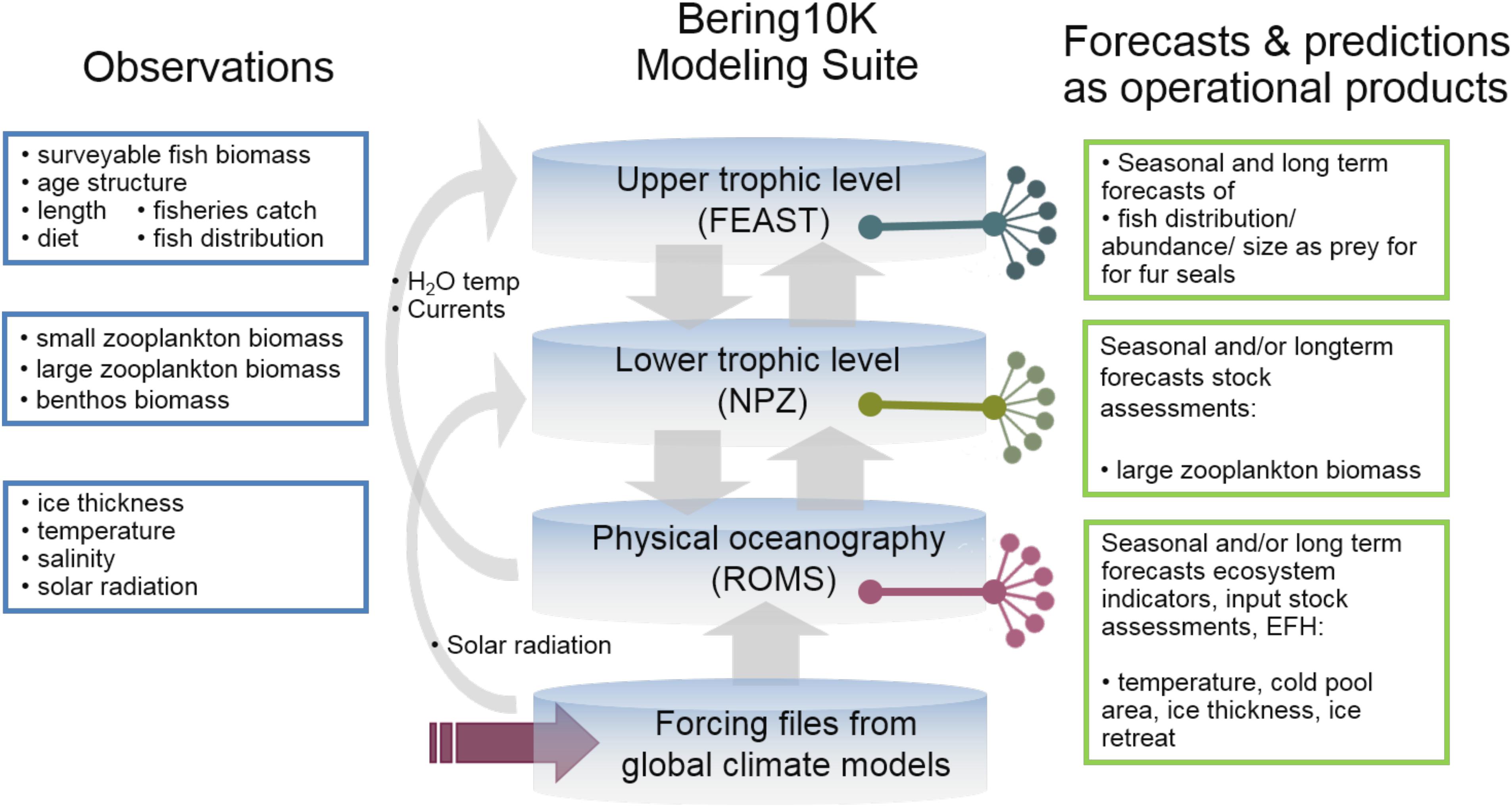
Figure 8. Bering 10K observational needs and products. Example of observations (left) used for validation of the Bering10 Modeling Suite as well as specific output from each module used in operational/testing products (right).

Skill and performance of the Bering10K modeling suite have been evaluated primarily over the eastern Bering Sea shelf using ocean in situ observations (Figure 8) and remotely sensed sea ice cover and ocean color data. Year-round vertical temperature and salinity profiles, as well as surface chlorophyll measurements, have been measured at four fixed moorings along the 70 m isobath on the Bering Sea shelf for the past 20+ years (Stabeno et al., 2012), and summertime hydrographic surveys span much of the southeastern shelf (Cokelet, 2016). These data have proven critical for model evaluation and improvement (Hermann et al., 2013, 2016; Ortiz et al., 2016). For instance, satellite and in situ observations pointed to warm biases in the modeled water column at an early stage of model development and led to improvements in the modeling of light attenuation (Kelly Kearney, personal communications); the mooring observations have allowed the detection of biases in the modeled vertical profiles of temperature and salinity, leading to the adjustment of the bulk flux algorithms used for surface heat and momentum fluxes. Observations have also been invaluable for understanding regional biophysical processes mechanistically (Cheng et al., 2014, 2015). Thus, the ability to evaluate, improve, and initialize the Bering10K forecasting systems depends critically on the availability of observational data, and on their spatial (both vertically and horizontally) coverage and temporal resolution (from synoptic to seasonal and multi-year time scales). For the physical model component, temperature and salinity profiles, mixed layer depth and sea ice are of particular importance. Observations are primarily available on the southeastern Bering Sea, while they are lacking on the Northern Bering Sea, Norton Sound, Bering Sea slope and the Aleutian Islands, creating uncertainties in the fidelity of the model simulation in those parts of the model domain. As the output of lower trophic levels is adopted or incorporated into more uses, assessment of phytoplankton and zooplankton abundance and phenology against observations are needed, particularly for ice algae, small and large phytoplankton, small copepods, large copepods, and krill. Observations of ocean acidification are available only for a few years, severely limiting the validation of the ocean acidification component. Finally, dissolved oxygen, though not a current issue in the Bering Sea, needs to be monitored to establish baseline patterns.

Novel Approaches to Large-Scale Ecosystem Monitoring in Support of Modeling Efforts

Ecological resources and associated ecosystem services are a key component of the Blue Economy, and ensuring sustainable use requires new and continued monitoring across multiple levels of biological organization. Monitoring biodiversity and ecological patterns improves our understanding of ecosystem dynamics, and supports conservation and management planning. In addition, ecological observations can provide input to physical/biogeochemical models and inspire alternative modeling approaches. Major roles in ecological monitoring are played by observing platforms (e.g., movebank, OTN, GEO BON, GOOS, OBIS, IMOS, Sea Around Us) that often provide freely accessible data for research purposes. However, such efforts can be spatiotemporally and taxonomically disjointed, while there is need for co-location of the ecological and physical/biogeochemical observations. Some approaches that have recently been used to provide a broad view of ecosystem composition as well as species and functions distribution, are described in the next sections.

Toward Holistic Marine Ecosystems Monitoring for Improving Ocean Models

Since 2009 the Tara Oceans international consortium, a partnership between academic scientists and the Tara Ocean Foundation¹¹, has developed an eco-systems biology approach for observing and analyzing planktonic ecosystems globally and over a broad range of scales. The Tara Oceans project is based on data derived from two circum-global research expeditions performed between 2009 and 2013 on board of a 36m long schooner (SV Tara) refitted to operate state-of-the-art oceanographic and plankton sampling equipment. The first expedition lasted 32 months, and sampled all of the principal ocean basins with the exception of the Arctic Ocean; the second lasted 6 months and circumnavigated the Arctic Circle. A wide range of contrasting ecosystems were targeted, and the shipboard activities collected environmental data and plankton of different sizes, for later analysis using state-of-the-art DNA sequencing and imaging technologies (Pesant et al., 2015; Lombardi et al., 2019).

The Tara Oceans program was designed to target well-defined mesoscale oceanographic features such as gyres, eddies, currents, frontal zones, upwellings, hotspots of biodiversity and low pH or low oxygen zones. SSH fields from AVISO (Archiving Validation and Interpretation of Satellite Data in Oceanography), as well as maps of SST from Operational Sea Surface Temperature and Sea Ice Analysis (OSTIA), and satellite-derived ocean color (ACRI-ST GlobColour service) were used to characterize the spatial and temporal variability of key environmental parameters along Tara’s track and select well defined sampling stations. In addition, Temperature-Salinity profiles available around sampling stations were compiled from the Argo autonomous network array, and a meteorological station mounted on board Tara continuously measured wind speed and direction, air temperature, pressure, and humidity. Real-time output from the Mercator Ocean model (see section Global Dynamical Models) was also used to characterize the daily environmental conditions. At a typical sampling station, plankton samples were collected from three environmentally distinct depths: surface layer, deep chlorophyll maximum layer, and mesopelagic (∼200–1000 m) zone.

The plankton sampled during the Tara Oceans expedition covers seven orders of magnitude in size (10 nm–10 cm), and includes all the organisms that form the bulk of biomass throughout the oceans, from viruses to zooplankton. The large number of samples obtained during the cruises (∼35,000 discrete samples) were later processed to obtain DNA/RNA information from the different size fractions, as well as information on the abundance, composition and morphological characteristics by combining different laboratory and in situ imaging instruments (e.g., size, shape, and optical density) of plankton and non-living suspended particles.

The holistic and systematic sampling implemented during the Tara Oceans expeditions was key for generating a comprehensive dataset that allowed to perform multi-parametric computational analyses similar to those being used in systems biology (Bork et al., 2015; Lombardi et al., 2019). The large number of biological samples and associated environmental data collected during the expedition have highlighted several important aspects of the functioning of plankton communities:

(1) There is a clear vertical stratification of epipelagic community composition at the global scale, which appears to be driven primarily by temperature (Sunagawa et al., 2015).

(2) A core set of prokaryotic gene families were found ubiquitously in the ocean and distinguished variable adaptive functions from stable core functions. High taxonomic variability is usually accompanied by relatively stable distributions of gene abundances summarized into functional categories. This observed functional redundancy across different taxa in microbial communities may confer a buffering capacity for the ecosystem in scenarios of biodiversity loss, and suggests that new biogeochemical models integrating prokaryotic omics information (i.e., information on biological molecules that influence organism functions, Louca et al., 2016) should rather consider key functions rather than species taxonomy. In addition to the stable abundance distribution of core functional processes, functional variations associated with non-core, adaptive gene families, are also detected. An example for such an environmental adaptation is provided by an increase of lipid metabolism in oxygen minimum zones of the Eastern Pacific and Northern Indian Ocean (Sunagawa et al., 2015), underlying the importance of monitoring specific genes at a global scale in the ocean.

(3) The large-scale nature of the plankton dataset enabled the analysis of the first global plankton interactome (i.e., predicted cross-kingdom ecological interactions, Lima-Mendez et al., 2015), leading to the surprising result that the plankton community structure appears to be shaped primarily by organism-organism interactions rather than by abiotic (e.g., physical environment) factors, which has important implications for ecosystem modeling where the forcing usually originates from physical (bottom–up) processes.

(4) The diversity of eukaryotic plankton is likely higher than that of prokaryotes and viruses (de Vargas et al., 2015), as is their functional gene complement (Carradec et al., 2018). While these organisms collectively harbor hundreds of millions of genes, some of them show potential to be used as markers for biogeochemical processes, e.g., diatom ISIP genes as markers of iron bioavailability (Kazamia et al., 2018; Caputi et al., 2019).

The above results point to the need for a modeling framework that integrates omics, morphological, and biogeochemical measurements to achieve an eco-systems understanding of the global ocean that incorporates its complexity from genes to meta-communities. The implementation of such a paradigm by Guidi et al. (2016) allowed the identification of specific plankton communities that played a major role in the biological carbon pump in the subtropical, nutrient-depleted oligotrophic ocean. This study also showed that the relative abundance of just a few bacterial and viral genes could explain a significant fraction of the variability in carbon export in these regions, underlying the power of omics biomarkers as proxies to monitor biogeochemical processes in the ocean.

However, the incorporation of omics information in global ocean models poses several challenges (i) because a conceptual framework (Figure 9) is still lacking for fully integrating omics knowledge into plankton ecosystem models (Stec et al., 2017) and (ii) because the number of omics-based biomarkers often remains too large to be directly incorporated as proper variables into ocean models (Tréguer et al., 2018). It is thus necessary to establish a roadmap toward fully integrated observations and their inclusion into operational tools. The roadmap should comprise the creation of omics augmented observatories, as suggested by the G7 working group on the “Future of Seas and Oceans,” allowing to support the development of a shared framework of new omics based indicators (e.g., the GLOMICON Initiative¹²) linked with Essential Ocean Variables (in support of GOOS), acting as a bridge toward a fully automated monitoring via biosensors. The MBON initiative¹³ has similar goals, and proposes that data be shared via http://www.iobis.org/. Conversely, the GEOTRACES international program, which aims to improve the understanding of biogeochemical cycles and large-scale distribution of trace elements and their isotopes in the marine environment¹⁴, is now considering how to incorporate omics into their standard operating procedures¹⁵. D’Alelio et al. (2018) have further proposed new types of data processing pipelines that could be used to generate new model configurations that combine the standard operational pipelines (e.g., ocean physics forecasting tools) with new genome-based models (Coles et al., 2017) or with predictors based on machine learning or other artificial intelligence tools (hybrid modeling, Figure 10).

FIGURE 9

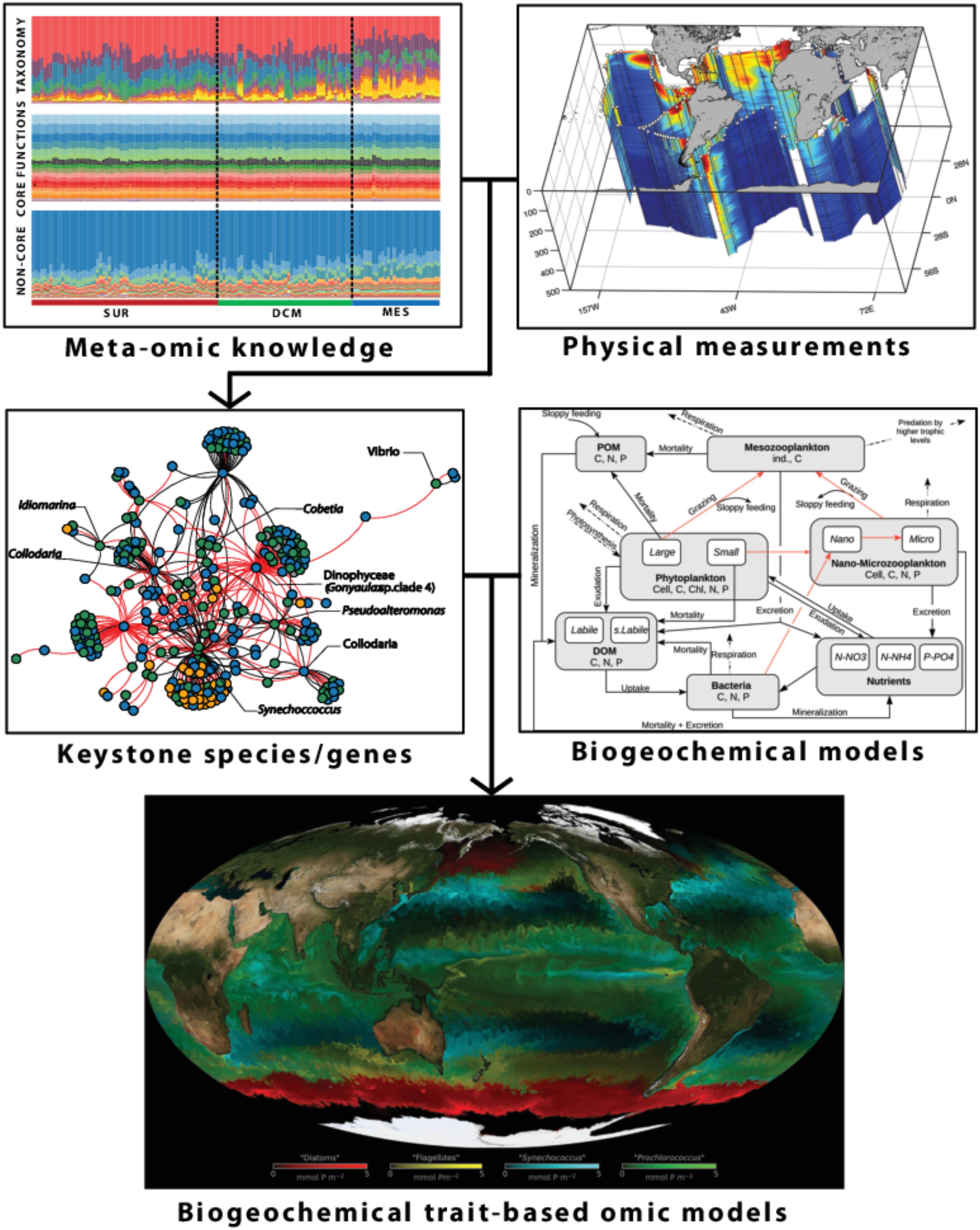
Figure 9. Meta-omics data based biogeochemical modeling. A schematic conceptual framework for global biogeochemical modeling from environmental, imaging, and meta-omics data (Sunagawa et al., 2015). A semi-automatic computational pipeline is schematized for combining biomarkers with biogeochemical data (Guidi et al., 2016) that can be incorporated into classic biogeochemical models (Guyennon et al., 2015) for creating a next generation of biogeochemical trait-based meta-omics models by considering their respective traits. Such novel meta-omics-enabled approaches aim to improve the monitoring and prediction of ocean processes while respecting the complexity of the planktonic system. For more information, see Louca et al. (2016) and Coles et al. (2017). The biogeochemical model is taken from https://www.biogeosciences.net/12/7025/2015/under a CC license (https://creativecommons.org/licenses/by/3.0/).

FIGURE 10

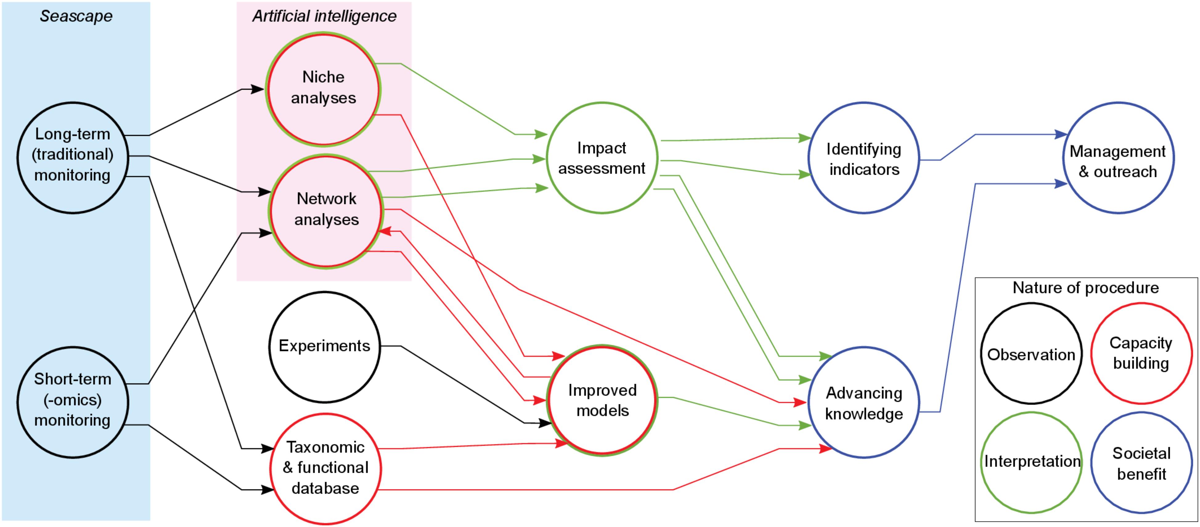
Figure 10. A proposed pipeline for omics-based plankton modeling and its potential implications. The conceptual-methodological pipeline aims at integrating traditional and omics observations over the long term within a framework exploiting high-standard computational approaches, such as niche and network analyses using artificial intelligence. These latter interpretative tools should stand at a high-level pipeline-position, i.e., at the intersection between data-providing nodes, and must be mutually calibrated and computationally merged by means of new-generation hybrid models. The latter should be fed by data processed by both taxonomic and functional databases exploiting omics resources and laboratory observations, which allow (i) generation of reference genomes for target organisms (selected for their key role or features) and (ii) developing experimental settings to characterize the growth dependencies of the same target organisms. Network analyses should also be applied to analyze model-output data pertaining to the dynamics of biological interaction networks. The final aim of this pipeline is to provide stakeholders with an intelligent assessment of ocean state, by developing interoperable ecological indicators and perpetually updatable monitoring protocols. For more information see D’Alelio et al. (2018).

In summary, the holistic monitoring undertaken by the Tara Oceans expedition has highlighted the use of systems biology approaches for studying and modeling the global ocean. To pursue future modeling efforts, this omics knowledge must be extended, together with physical and chemical measurements, to all oceanic provinces that are undergoing significant stress (e.g., oxygen-depletion and/or low pH). Surveys in these regions may allow the discovery of new metabolic potentials that could be of interest for the Blue Economy. Today, the cost of omics sampling is continuously decreasing and is also becoming more and more portable, which should enable sampling at the mesoscale. Other activities should focus on high-resolution time series to improve our understanding of the dynamics of biogeochemical processes and ecological interactions in the context of anthropogenic global change (Hastings et al., 2018). This new sampling will be key to distinguish acclimation versus adaptation processes of plankton in the context of climate change, giving ocean studies the opportunity to integrate ecosystem behaviors into new climate models, scenarios and projections.

Using Acoustic Data to Understand the Dynamics of Mesopelagic Fish Species

Mesopelagic fish refers to the species living in the 200–1000 m depth range. The potentially huge biomass of mesopelagic fish at a global scale has raised interest in the exploitation of this resource as a potential for “blue growth” (St. John et al., 2016). However, without a good knowledge of the biomass and dynamics of these species, as well as in-depth understanding of the role they play in the global ecosystem dynamics the development of such exploitation could have devastating impacts on the whole ecosystem structure. These mesopelagic species, or “mesopelagics,” support the large diversity of predator species. They may also substantially contribute to the “biological pump” through their vertical diel migrations (Davison et al., 2015). Thus, more extensive research and monitoring efforts are needed to estimate this marine biomass and its dynamics, and to incorporate these results in marine ecosystem models. The latter can then be used to explore ecosystem dynamics and for prediction purposes. A priority is to develop routine in situ observations and monitoring of global marine biomass to estimate marine ecosystem dynamics and changes on a global scale (Nymand-Larson et al., 2014).

Acoustic-trawl surveying is a standardized method to provide information on fish abundance for fish stock assessment (see e.g., Mac Lennan and Simmonds, 2005). The method requires trawl sampling to support the acoustic measurements since species type, length and age estimates are required for the conventional assessment models. The technique utilizes the fact that different fish size and taxa have different acoustic reflectivities as a function of frequency, and this is used to aid the interpretation of the measurements, and the “allocation” of acoustic backscattered energy to various species. However, the method is expensive and can only be realistically deployed for economically important species. For a global mesopelagic observation system, it is not feasible due to the trawl sampling requirements. More recently, acoustic transects without trawls have been used (Irigoien et al., 2014; Davison et al., 2015). This results in a lower taxonomic resolution, where age and size resolution is lost or is significantly more difficult to assess. However, this approach enables the use of other platforms, such as buoys, vessels of opportunity, wave gliders etc., and thus leads to a much better coverage that is possible with the traditional fisheries acoustics method. If models can be developed to efficiently utilize this information (e.g., Lehodey et al., 2015; Proud et al., 2017), it would mean a significant step forward in terms of our understanding of the ocean dynamics and how the lower trophic levels are linked to trophic levels used for human consumption.

MESOPP (Mesopelagic Southern Ocean Prey and Predators), a European International Cooperation project, having just finished its initial 3-year plan, aims to advance international collaboration in observing mesopelagic biota using active acoustics in a Global Sampling Network to support modeling of the Mid-High Trophic Levels of Ocean Ecosystems. MESOPP, initially a collaboration in the Southern Ocean (SO), developed a public e-infrastructure with standardized acoustic data to allow estimation of the biomass of mesopelagic biota, and used these to improve and validate ecosystem models¹⁶. The priority has been to develop the datasets, methods and models needed to simulate and quantify the dynamics and functional roles of these communities. This activity has global value. Thus, the MESOPP consortium would like to expand this work to the Global Oceans. It has developed methods and data standards that can be easily used elsewhere. MESOPP has found international interest in combining advances in ecosystem modeling with those in acoustic sciences to propose a coupled observation-modeling system to generate new knowledge, enable quantification of ecosystem processes and dynamics, and in the long-term form the basis for ecosystem assessments. Its results suggest that the incorporation of acoustic information into ecosystem models would require the development of acoustic observation models, the definition of eco-regions inhabited by homogeneous species communities (in regard to their responses to acoustic signals), and a limited number of reference stations of those regions providing accurate estimates of absolute biomass. Genomics have also been identified as a promising approach to characterize species communities that characterize eco-acoustic provinces. While multi-frequency technology is developing, a first global dataset of one single frequency (38 kHz) could be achieved from existing archived research cruise data and planned initiatives.

Acoustic observation models are the first key step needed to translate acoustic signals into predicted biomass. This acoustically derived biomass can then be compared with the biomass predicted by ecosystem models, or alternatively used to convert the model biomass into a predicted acoustic signal to be compared directly with acoustic observations. This is particularly important since some organisms contribute relatively more to the total backscattered energy than others. Acoustic energy is not a linear function of biomass, and if these latter groups are not separated in the model, the uncertainty in the conversion using the acoustic observation model will be high. Once biomass is estimated it can be used to validate ecosystem models that include a representation of these groups of organisms (Christensen and Walters, 2004; Lehodey et al., 2010; Fulton et al., 2011; Lefort et al., 2014; Blanchard et al., 2017). Biomass estimates can even be used to directly optimize the model parameters. Such an approach has been developed for the Mid-trophic level (MTL) component (Lehodey et al., 2010) of the SEAPODYM model (Lehodey et al., 2008) that includes functional groups of vertically migrating and non-migrating mesopelagic micronekton organisms (Figure 11). The overall biomass is controlled by energy transfer coefficients that can be estimated using acoustic data (Lehodey et al., 2015), thanks to a Maximum Likelihood Estimation approach that uses the adjoint technique with the quasi-Newton gradient method to minimize the cost function (Senina et al., 2008). Results from this research will provide a deeper understanding of mesopelagic species behavior and dynamics within the broader ecosystem communities, and develop models that can realistically simulate that behavior.

FIGURE 11

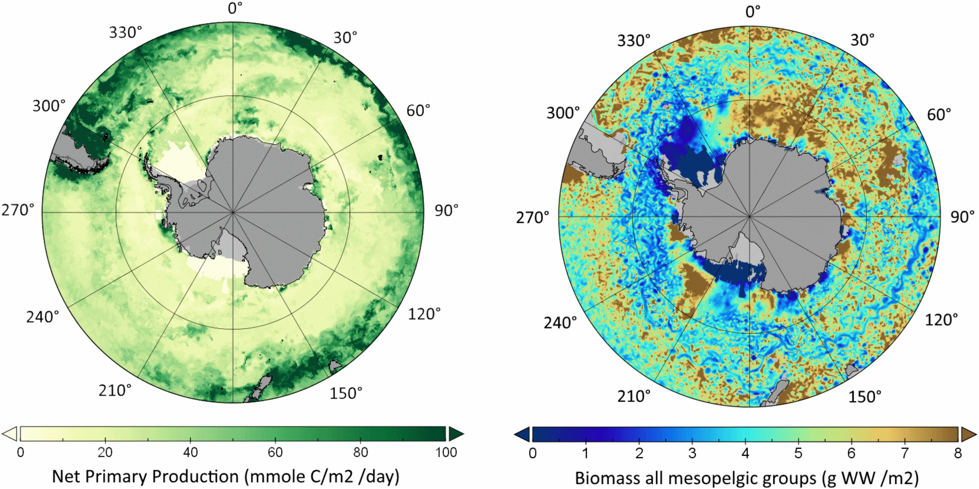
Figure 11. Lower and mid trophic levels in the Southern Ocean. Comparison of (left) primary production derived from satellite ocean color data and (right) predicted mesopelagic micronekton biomass with the model SEAPODYM for the first week of January 2016. The distribution is the sum of biomass of 5 functional groups characterized either as resident or undertaking diel vertical migrations, and simulated from primary production, ocean circulation and temperature (Lehodey et al., 2010, 2015). White color indicates sea ice coverage. See www.mesopp.eu for access to data and model outputs.

Seascapes

Contextualizing high-resolution taxonomic measurements and improving the parameterization of marine ecosystem models both benefit from the use of some sort of biogeographic framework (e.g., Longhurst, 1998; Oliver and Irwin, 2008; Platt and Sathyendranath, 2008; Kavanaugh et al., 2014, 2016). Terrestrial and marine benthic ecology draw from landscape ecology to address issues of complexity, patchiness, and scale (e.g., Paine and Levin, 1981; Steele, 1991; Levin, 1992; Schneider, 2001), as well as spatial context sampling bias, and edge effects (Turner, 2005). The marine environment can also be viewed as a mosaic of distinct seascapes, with unique combinations of biological, chemical, geological, and physical processes that define habitats which change over time (Steele, 1991; Karl and Letelier, 2009; Kavanaugh et al., 2014). Indeed, partitioning of the ocean surface has occurred based on multivariate surface properties including ocean color (e.g., Longhurst et al., 1997), trophic potential (diatom and chl-a abundance, Sathyendranath et al., 2004; Platt and Sathyendranath, 2008), temperature and salinity profiles (Hooker et al., 2000), as well as known distributions of species. Recently, Sayre et al. (2017) classified distinct volumetric Ecological Marine Units (EMUs) using multidecadal climatologies of nutrients, temperature, and salinity from the World Ocean Atlas (Garcia et al., 2013; Locarnini et al., 2013). The EMU process recognizes that marine ecosystems are not two dimensional, but operate as 3D (e.g., through the water column) entities (e.g., Li and Gold, 2004; Wright et al., 2007).

The oceanographic and fisheries management communities have recognized that climatologies do not adequately characterize dynamic ocean ecosystems (Oliver and Irwin, 2008; Hardman-Mountford et al., 2009; Dutkiewicz et al., 2012; Kavanaugh et al., 2016). There have thus been efforts to classify surface seascapes on seasonal, interannual, and multiple spatial scales using model and satellite remote sensing data. Seasonal dynamics for coastal regions have been inferred with dynamic but discontinuous boundaries (Saraceno et al., 2006; Devred et al., 2007) or by explicitly including seasonal and spatial forcing in their assessments (Hales et al., 2012). Others have applied post hoc classifications based on distributions of variables within subjective Longhurst Province boundaries on seasonal and annual scales (e.g., Reygondeau et al., 2013). Objective and dynamic seascapes have been classified using satellite remote sensing data on basin (Kavanaugh et al., 2014) and global (Oliver and Irwin, 2008; Irwin and Oliver, 2009) scales by simultaneously clustering pixels in space and time. Each of these methods assumes that seascapes have unique multivariate distributions, that there are natural discontinuities or gradients that delimit seascapes, and that the boundaries change with time. Thus, modern seascape classification merges lower trophic level ecology, geography, and ocean dynamics using observations that are updated regularly and that provide a historical context as reference against which to measure change. An example of seascape evolution in the Northern California Current is shown in Figure 12.

FIGURE 12

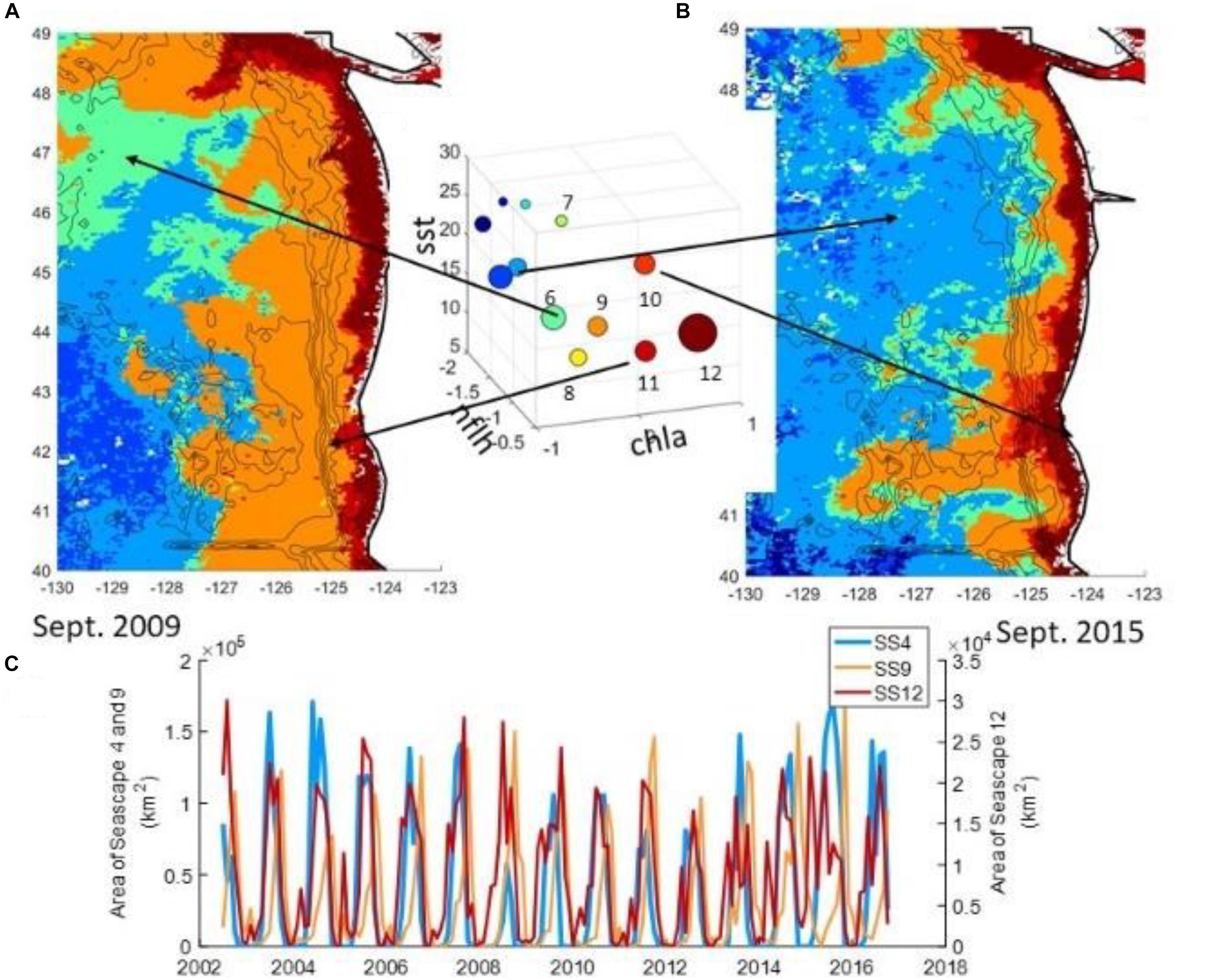
Figure 12. Seascape evolution in the Northern California Current. Seascapes were classified as per Kavanaugh et al. (2014, 2016), using synoptic time series of Aqua-MODIS SST (in °C), chl-a, in units of log₁₀(mg m^–3), and normalized fluorescent line height (nflh), in units of log₁₀(W m^–2 μm^–1 sr^–1). (A,B) Show snapshots of seascape identity for September of 2009 and 2015 respectively; (C) shows time series of areal extent of 3 of a total of 12 seascapes. While both years show high production very near shore (seascape 12), note the loss of North Pacific transition water (green, seascape 6) and intrusion of oligotrophic water (blues, seascape identity ≤ 5) on the shelf in 2015. The areal extent of California Current Shelf water (orange, seascape 9) also decreases in 2015. Warm productive water (seascape 10), is normally found south of Point Conception, CA.

Seascape and provincial divisions have been useful for better parameterizing and identifying mechanistic relationships within complex marine ecosystem models (e.g., Dutkiewicz et al., 2012; Hales et al., 2012). For example, Hales et al. (2012) were better able to constrain a semi-mechanistic model of the carbonate system in the California current, with reduced error and reliance on non-mechanistic predictor variables. Kavanaugh et al. (2017) and Rheuban et al. (2017) were able to better predict benthic temperature trends and drivers along the NE continental shelf by first applying a seascape classification that characterized the seasonal shape of water column temperature gradients. Plankton and bacterioplankton community structure are different across dynamic seascapes (Gomez-Pereira et al., 2010; Kavanaugh et al., 2015), with ongoing efforts to validate seascape patterns at higher trophic levels, including endangered species, such as Atlantic Sturgeon (Breece et al., 2016).

In the U.S., three pilot Marine Biodiversity Observing Network (MBON; Duffy et al., 2013; Muller-Karger et al., 2014) were established through a partnership established between NASA, NOAA, the Bureau of Ocean Energy Management (BOEM), the Smithsonian Institution’s Tennenbaum Marine Observatories Network, and the Ocean Biogeographic Information System (OBIS). The pilot MBONs are located in tropical reef environments, coastal upwelling regions, and polar ecosystems, and represent a step toward integrating multivariate oceanographic and multitrophic level ecological data in an organized, multi-scale framework. Objective classification and validation of remotely sensed dynamic seascapes using high resolution (1 km) satellite data has occurred at regional to local scales as part of the US MBON pilot program. Seascapes provide a framework to assess and scale up patterns of biodiversity and effects of environmental change on pelagic community structure, ranging from microbes to fish, and provide indicators of habitat quality to inform marine ecosystem management. In concert with ship, buoy, and autonomous platform measurements, seascapes categories are being used as an objective extent to plan sampling, conduct rarefaction studies, intercompare spatial and temporal patterns across trophic levels, test hypotheses of fisheries habitat affinities (e.g., Santora et al., 2012), quantify habitat diversity (Whitaker, 1977; Turner, 2005), and examine temporal shifts in habitat quality and availability within existing jurisdictional units.

Conclusion

In this paper, we have provided an overview of a broad range of state-of-the-art approaches for sampling, modeling, and forecasting marine ecosystems, and their observational needs at the development, initialization and validation stages. We have primarily focused on modeling and forecasting activities in regions near the U.S. coasts, whose diversity illustrates the possible different sources of predictability and the observations needed to capture those differences. These efforts are essential for supporting ecosystem services as well as the Blue Economy. The examples presented in this paper range from very high-resolution regional models to global physical or coupled physical-biogeochemical models of different spatial resolution. Statistical approaches for modeling and forecasting key physical ecosystem drivers have also been discussed. Important insights on observational needs to sustain and advance these diverse efforts have emerged from this review, and are summarized here below.

Global physical models with sufficiently high spatial resolution to resolve coastal features are essential for understanding the connection between regional processes and large-scale climate variations, as they seamlessly simulate the interaction among these different scales. The development and validation of these models at the regional scale relies on high-resolution observations in the area of interest (as seen, e.g., in the Northwest Atlantic, see section Modeling the Northwest Atlantic). At the same time, high-resolution global-scale fields, like SST and SSH data sets obtained from satellite missions, are also key for the development and validation of the models at the large scale.

Global biogeochemical models are strongly limited by the sparsity of biogeochemical data to be used for model initialization, leading to a very long spin-up time of biogeochemical variables, and to a possible mismatch between biogeochemistry and physics. The short record of biogeochemical data, whose duration is generally insufficient to even define a regional climatology for the biogeochemical variables, is another important limiting factor in model validation [e.g., Chlorophyll distribution in the CCS, see section Assessing the Physical-Biogeochemical Response of the California Current System (CCS) to ENSO]. A sustained deployment of Bio-Geochemical Argo floats, as well as a continuation of satellite missions providing global measurements of ocean color can be expected to help mitigate the issues associated with the initialization and validation of the global biogeochemical models. High-resolution physical and biogeochemical observations near coastal regions are key to capture the important small-scale features of these quantities.

Empirical dynamical models (e.g., Linear Inverse Models, see section Linear Inverse Models) and other statistical approaches [e.g., synoptic meteorology (see section Synoptic Meteorology and Coastal Applications) and multiple linear regressions (see section Temperature Predictions in the Northwest Atlantic)] have also proved to be very valuable tools for seasonal forecasts. These approaches rely on statistical relationships between predictands and predictors, which themselves exploit the dynamical processes linking aspects of the ecosystem to climate, and whose nature may be location dependent. For these types of applications, the duration and consistency of the data record is critical for the determination of robust statistical relationships between predictands and predictors. For LIM applications, SSH has proven to be an extremely valuable quantity for capturing the dynamics of the system and improving the forecast skill, calling for a continuation of altimetry observations.

The high-resolution regional forecasting activities presented in this paper (i.e., the J-SCOPE and Bering Sea projects) have succeeded in producing skillful seasonal forecasts relevant to fisheries, thanks to the availability of continuous observations used for model development and validation, as well as for forecast verification. Biases in these products originate primarily from the biases of the global forecast systems that provide the lateral boundary conditions and the surface forcing to the physical regional model component. Moving forward, specific observations particularly critical for the biogeochemical forecasting of these regional models include:

(1) Subsurface observations, which are very important for initialization and boundary conditions.

(2) Sediment information, needed for evaluating the evolution of changes in oxygen, carbon, and nutrients.

(3) Information on rates, needed to constrain some processes (e.g., net primary productivity, calcification) as well as to validate model prediction of biogeochemical quantities (e.g., oxygen).

(4) Terrestrial inputs (e.g., river runoff, non-point source input of nutrients along the coast), needed for estimating stratification as well as nutrient dynamics.

Novel approaches to physical and biogeochemical monitoring are becoming available and may provide new insights into ecosystem evolution and change at a large-to-global scale. These approaches include the morpho-genetic characterization of ecosystems (e.g., Tara Oceans), the identification of “seascapes,” and the monitoring of mesopelagic fish at a global scale to understand their role in ecosystem dynamics and in the carbon cycle (MESOPP consortium). The value of these approaches lies in their holistic nature that encompasses physical and biological aspects; they may provide a potentially powerful way to monitor the ecosystem and its evolution in a rapidly changing ocean environment. However, the incorporation of these holistic approaches in current state-of-the-art models may be challenging given the differences in approach and number of variables. Thus, an ongoing dialog between these communities needs to take place to identify a common language and operating platform. This is already happening in the examples cited, and these exploratory attempts are likely to catalyze a paradigm shift in ocean monitoring in the coming decades.

Author Contributions

All authors listed have made a substantial, direct and intellectual contribution to the work, and approved it for publication.

Conflict of Interest

The authors declare that the research was conducted in the absence of any commercial or financial relationships that could be construed as a potential conflict of interest.

Funding

This study was supported by the NOAA’s Climate Program Office’s Modeling, Analysis, Predictions, and Projections (MAPP) Program through grants NA17OAR4310106, NA17OAR4310104, NA17OAR4310108, NA17OAR4310109, NA17OAR4310110, NA17OAR4310111, NA17OAR4310112, and NA17OAR4310113. This manuscript is a product of the NOAA/MAPP Marine Prediction Task Force. The Tara Oceans consortium acknowledges support from the CNRS Research Federation FR2022 Global Ocean Systems Ecology and Evolution, and OCEANOMICS (grant agreement ‘Investissement d’Avenir’ ANR-11-BTBR-0008). This is article number 95 of the Tara Oceans consortium. MK and SD acknowledge support from NASA grant NNX14AP62A “National Marine Sanctuaries as Sentinel Sites for a Demonstration Marine Biodiversity Observation Network (MBON)” funded under the National Ocean Partnership Program (NOPP RFP NOAA-NOS-IOOS-2014-2003803 in partnership between NOAA, BOEM, and NASA), and the NOAA Integrated Ocean Observing System (IOOS) Program Office. WC, IO, and AH acknowledge partial support from the Joint Institute for the Study of the Atmosphere and Ocean (JISAO) under NOAA Cooperative Agreement NA15OAR4320063, Contribution No. 2019-1029. This study received support from the European H2020 International Cooperation project MESOPP (Mesopelagic Southern Ocean Prey and Predators), grant agreement no. 692173.

Acknowledgments

We would like to thank J. D. Scott and E. Norton for their help in preparing some of the figures, and C. Stock for his precious input on global biogeochemical modeling. We would also like to thank the three reviewers, whose excellent suggestions and very constructive criticism have greatly improved the manuscript. The Surface Ocean CO₂ Atlas (SOCAT) is an international effort, endorsed by the International Ocean Carbon Coordination Project (IOCCP), the Surface Ocean Lower Atmosphere Study (SOLAS) and the Integrated Marine Biosphere Research (IMBeR) program, to deliver a uniformly quality-controlled surface ocean CO₂ database. The many researchers and funding agencies responsible for the collection of data and quality control are thanked for their contributions to SOCAT.

Footnotes

1. ^ https://oceansolutions.stanford.edu/project-ocean-tipping-points
2. ^ https://www.godae-oceanview.org
3. ^ https://www.mercator-ocean.fr
4. ^ https://www.nemo-ocean.eu
5. ^ https://www.aviso.altimetry.fr
6. ^ http://www.nanoos.org/products/j-scope/
7. ^ https://www.nprb.org/bering-sea-project/
8. ^ https://www.integratedecosystemassessment.noaa.gov/regions/alaska/ebs-integrated-modeling
9. ^ https://www.npfmc.org/bsfep/
10. ^ http://www.lenfestocean.org/en/news-and-publications/fact-sheet/new-research-to-examine-relationships-between-northern-fur-seals-pollock-and- climate-change-in-alaska
11. ^ https://www.embl.de/tara-oceans/start/
12. ^ https://github.com/GLOMICON/omicon
13. ^ http://www.marinebon.org/
14. ^ http://www.geotraces.org/
15. ^ https://www.biogeoscapes.org/
16. ^ www.mesopp.eu

References

Bakker, D. C. E., Pfeil, B., Landa, C. S., Metzl, N., O’Brien, K. M., Olsen, A., et al. (2016). A multi-decade record of high-quality fCO₂ data in version 3 of the Surface Ocean CO₂ Atlas (SOCAT). Earth Sys. Sci. Data 8, 383–413. doi: 10.5194/essd-8-383-2016

CrossRef Full Text | Google Scholar

Banas, N. S., Lessard, E., Kudela, R., MacCready, P., Peterson, T., Hickey, B. M., et al. (2009). Planktonic growth and grazing in the Columbia River plume region: a biophysical model study. J. Geophys. Res. 114:C00B06. doi: 10.1029/2008JC004993

CrossRef Full Text | Google Scholar

Becker, E., den Dool, H., and Zhang, Q. (2014). Predictability and forecast skill in NMME. J. Clim. 27, 5891–5906. doi: 10.3389/fmicb.2017.01291

PubMed Abstract | CrossRef Full Text | Google Scholar

Becker, E. A., Forney, K. A., Redfern, J. V., Barlow, J., Jacox, M. G., Roberts, J. J., et al. (2019). Predicting cetacean abundance and distribution in a changing climate. Div. Distrib. 25, 626–643. doi: 10.1111/ddi.12867

CrossRef Full Text | Google Scholar

Bednarsek, N., Feely, R. A., Tolimieri, N., Hermann, A. J., Siedlecki, S. A., Waldbusser, G. G., et al. (2017). Exposure history determines pteropod vulnerability to ocean acidification along the US West Coast. Sci. Rep. 7:4526. doi: 10.1038/s41598-017-03934-z

PubMed Abstract | CrossRef Full Text | Google Scholar

Blanchard, J. L., Heneghan, R. F., Everett, J. D., Trebilco, R., and Richardson, A. J. (2017). From bacteria to whales: using functional size spectra to model marine ecosystems. Trends Ecol. Evol. 32, 174–186. doi: 10.1016/j.tree.2016.12.003

PubMed Abstract | CrossRef Full Text | Google Scholar

Bograd, S. J., Castro, C. G., Di Lorenzo, E., Palacios, D. M., Bailey, H., Gilly, W., et al. (2008). Oxygen declines and the shoaling of the hypoxic boundary in the California current. Geophys. Res. Lett. 35:L12607. doi: 10.1029/2008GL034185

CrossRef Full Text | Google Scholar

Bork, P., Bowler, C., de Vargas, C., Gorsky, G., Karsenti, E., and Wincker, P. (2015). Tara Oceans studies plankton at planetary scale. Science 348:873. doi: 10.1126/science.aac5605

PubMed Abstract | CrossRef Full Text | Google Scholar

Bowen, R. E., and Riley, C. (2003). Socio-economic indicators and integrated coastal management. Ocean Coast. Manag. 46, 299–312. doi: 10.1016/s0964-5691(03)00008-5

CrossRef Full Text | Google Scholar

Brady, R. X., Lovenduski, N. S., Alexander, M. A., Jacox, M., and Gruber, N. (2018). On the role of climate modes in modulating the air-sea CO2 fluxes in Eastern boundary upwelling systems. Biogeosciences 16, 329–346. doi: 10.5194/bg-2018-415

CrossRef Full Text | Google Scholar

Breece, M. W., Fox, D. A., Dunton, K. J., Frisk, M. G., Jordaan, A., and Oliver, M. J. (2016). Dynamic seascapes predict the marine occurrence of an endangered species: Atlantic Sturgeon Acipenser oxyrinchus oxyrinchus. Methods Ecol. Evol. 7, 725–733. doi: 10.1111/2041-210x.12532

CrossRef Full Text | Google Scholar

Brodie, S., Jacox, M. G., Bograd, S. J., Welch, H., Dewar, H., Scales, K. L., et al. (2018). Integrating dynamic subsurface habitat metrics into species distribution models. Front. Mar. Sci. 5:219. doi: 10.3389/fmars.2018.00219

CrossRef Full Text | Google Scholar

Capotondi, A., Alexander, M. A., Bond, N. A., Curchitser, E. N., and Scott, J. D. (2012). Enhanced upper ocean stratification with climate change in the CMIP3 models. J. Geophys. Res. Oceans 117:C04031. doi: 10.1029/2011JC007409

CrossRef Full Text | Google Scholar

Capotondi, A., and Sardeshmukh, P. D. (2015). Optimal precursors of different types of ENSO events. Geophys. Res. Lett. 42, 9952–9960. doi: 10.1002/2015gl066171

CrossRef Full Text | Google Scholar

Capotondi, A., and Sardeshmukh, P. D. (2017). Is El Niño really changing? Geophys. Res. Lett. 44, 8548–8556. doi: 10.1002/2017GL074515

CrossRef Full Text | Google Scholar

Capotondi, A., Wittenberg, A. T., Newman, M., Di Lorenzo, E., Yu, J.-Y., Braconnot, P., et al. (2015). Understanding ENSO diversity. Bull. Am. Meteorol. Soc. 96, 921–938.

Google Scholar

Caputi, L., Carradec, Q., Eveillard, D., Kirilovsky, A., Pelletier, E., Pierella Karlusich, J. J., et al. (2019). Community-level responses to iron availability in open ocean plankton ecosystems. Glob. Biogeochem. Cycles 33, 391–419. doi: 10.1029/2018GB006022

CrossRef Full Text | Google Scholar

Carradec, Q., Pelletier, E., Da Silva, C., Alberti, A., Seeleuthner, Y., Blanc-Mathieu, R., et al. (2018). A global ocean atlas of eukaryotic genes. Nat. Commun. 9:373. doi: 10.1038/s41467-017-02342-1

PubMed Abstract | CrossRef Full Text | Google Scholar

Chan, F., Barth, J. A., Blanchette, C. A., Byrne, R. H., Chavez, F., Cheriton, O., et al. (2017). Persistent spatial structuring of coastal ocean acidification in the California current system. Sci. Rep. 7:2526. doi: 10.1038/s41598-017-02777-y

PubMed Abstract | CrossRef Full Text | Google Scholar

Chan, F., Chornesky, E. A., Klinger, T., Largier, J. L., Wakefield, W. W., and Whiteman, E. A. (2016). Supporting Ecological Resilience to Address Ocean Acidification and Hypoxia. Oakland, CA: California Ocean Science Trust.

Google Scholar

Chavez, F. P., Collins, C. A., Huyer, A., and Mackas, D. L. (2002). El Niño along the west coast of North America, Editorial. Prog. Oceanogr. 54, 1–5. doi: 10.1016/s0079-6611(02)00040-x

CrossRef Full Text | Google Scholar

Chavez, F. P., and Messié, M. (2009). A comparison of eastern boundary upwelling ecosystems. Prog. Oceanogr. 83, 80–96. doi: 10.7717/peerj.5339

PubMed Abstract | CrossRef Full Text | Google Scholar

Chavez, F. P., Ryan, J., Lluch-Cota, S. E., and Ñiquen, M. (2003). From anchovies to sardines and back: multidecadal change in the Pacific Ocean. Science 299, 217–221. doi: 10.1126/science.1075880

PubMed Abstract | CrossRef Full Text | Google Scholar

Checkley, D. M. Jr., and Barth, J. A. (2009). Patterns and processes in the California current system. Prog. Oceanogr. 83, 49–64. doi: 10.1016/j.pocean.2009.07.028

CrossRef Full Text | Google Scholar

Chen, K., Gawarkiewicz, G. G., Kwon, Y.-O., and Zhang, W. G. (2015). The role of atmospheric forcing versus ocean advection during the extreme warming of the Northeast US continental shelf in 2012. J. Geophys. Res. Oceans 120, 3522–3541.

Google Scholar

Chen, K., Gawarkiewicz, G. G., Lentz, S. J., and Bane, J. M. (2014). Diagnosing the warming of the northeastern US coastal ocean in 2012: a linkage between the atmospheric jet stream variability and ocean response. J. Geophys. Res. Oceans 119, 218–227. doi: 10.1002/2013jc009393

CrossRef Full Text | Google Scholar

Chen, K., Kwon, Y.-O., and Gawarkiewicz, G. G. (2016). Interannual variability of winter-spring temperature in the Middle Atlantic Bight: relative contributions of atmospheric and oceanic processes. J. Geophys. Res. Oceans 121, 4209–4227. doi: 10.1002/2016jc011646

CrossRef Full Text | Google Scholar

Cheng, W., Curchitser, E., Ladd, C., Stabeno, P., and Wang, M. (2014). Influences of sea ice on the Eastern Bering Sea: NCAR CESM simulations and comparison with observations. Deep Sea Res. Part II Top. Stud. Oceanogr. 109, 27–38. doi: 10.1016/j.dsr2.2014.03.002

CrossRef Full Text | Google Scholar

Cheng, W., Curchitser, E., Stock, C., Hermann, A., Cokelet, E., Mordy, C., et al. (2015). What processes contribute to the spring and fall bloom co-variability on the Eastern Bering Sea shelf? Deep-Sea Res. II 134, 128–140. doi: 10.1016/j.dsr2.2015.07.009

CrossRef Full Text | Google Scholar

Cheung, W. W., Lam, V. W., Sarmiento, J. L., Kearney, K., Watson, R., and Pauly, D. (2009). Projecting global marine biodiversity impacts under climate change scenarios. Fish Fish. 10, 235–251. doi: 10.1111/j.1467-2979.2008.00315.x

CrossRef Full Text | Google Scholar

Cheung, W. W., Lam, V. W., Sarmiento, J. L., Kearney, K., Watson, R. E. G., Zeller, D., et al. (2010). Large-scale redistribution of maximum fisheries catch potential in the global ocean under climate change. Glob. Change Biol. 16, 24–35. doi: 10.1111/j.1365-2486.2009.01995.x

CrossRef Full Text | Google Scholar

Christensen, V., and Walters, C. J. (2004). Ecopath with ecosim: methods, capabilities and limitations. Ecol. Model. 172, 109–139. doi: 10.1016/j.ecolmodel.2003.09.003

CrossRef Full Text | Google Scholar

Cloern, J. E., Abreu, P. C., Carstensen, J., Chauvaud, L., Elmgren, R., Grall, J., et al. (2016). Human activities and climate variability drive fast-paced change across the world’s estuarine–coastal ecosystems. Glob. Change Biol. 22, 513–529. doi: 10.1111/gcb.13059

PubMed Abstract | CrossRef Full Text | Google Scholar

Cokelet, E. D. (2016). 3-D water properties and geostrophic circulation on the eastern Bering sea shelf. Deep-Sea Res. II 134, 65–85. doi: 10.1016/j.dsr2.2016.08.009

CrossRef Full Text | Google Scholar

Coles, V. J., Stukel, M. R., Brooks, M. T., Burd, A., Crump, B. C., Moran, M. A., et al. (2017). Ocean biogeochemistry modeled with emergent trait-based genomics. Science 358, 1149–1154. doi: 10.1126/science.aan5712

PubMed Abstract | CrossRef Full Text | Google Scholar

Cossarini, G., Mariotti, L., Feudale, L., Mignot, A., Salon, S., Taillandier, V., et al. (2018). Towards operational 3D-Var assimilation of chlorophyll Biogeochemical Argo float data into a biogeochemical model of the Mediterranean Sea. Ocean Model. 133, 112–128. doi: 10.1016/j.ocemod.2018.11.005

CrossRef Full Text | Google Scholar

Coyle, K. O., Eisner, L. B., Mueter, F. J., Pinchuk, A. I., Janout, M. A., Cieciel, K. D., et al. (2011). Climate change in the southeastern Bering Sea: impacts on pollock stocks and implications for the oscillating control hypothesis. Fish. Oceanogr. 20, 139–156. doi: 10.1111/j.1365-2419.2011.00574.x

CrossRef Full Text | Google Scholar

D’Alelio, D., Eveillard, D., Coles, V. J., Caputi, L., Ribera d’Alcalà, M., and Iudicone, D. (2018). Modelling the complexity of plankton communities exploiting omics potential: from present challenges to an integrative pipeline. Curr. Opin. Syst. Biol. 13, 68–74. doi: 10.1016/j.coisb.2018.10.003

CrossRef Full Text | Google Scholar

Davis, K. A., Banas, N. S., Giddings, S. N., Siedlecki, S. A., Maccready, P., Lessard, E. J., et al. (2014). Estuary-enhanced upwelling of marine nutrients fuels coastal productivity in the U.S. Pacific Northwest. J. Geophys. Res. Oceans 119, 8778–8799. doi: 10.1002/2014JC010248

CrossRef Full Text | Google Scholar

Davison, P. C., Koslow, J. A., and Kloser, R. J. (2015). Acoustic biomass estimation of mesopelagic fish: backscattering from individuals, populations, and communities. ICES J. Mar. Sci. 72, 1413–1424. doi: 10.1093/icesjms/fsv023

CrossRef Full Text | Google Scholar

de Vargas, C., Audic, S., Henry, N., Decelle, J., Mahé, F., Logares, R., et al. (2015). Ocean plankton. Eukaryotic plankton diversity in the sunlit ocean. Science 348:1261605. doi: 10.1126/science.1261605

PubMed Abstract | CrossRef Full Text | Google Scholar

Devred, E., Sathyendranath, S., and Platt, T. (2007). Delineation of ecological provinces using ocean colour radiometry. Mar. Ecol. Prog. Ser. 346, 1–13. doi: 10.3354/meps07149

CrossRef Full Text | Google Scholar

Dias, D. F., Subramanian, A., Zanna, L., and Miller, A. J. (2018). Remote and local influences in forecasting Pacific SST: a linear inverse model and a multimodel ensemble study. Clim. Dyn. 52, 3183–3201. doi: 10.1007/s00382-018-4323-z

CrossRef Full Text | Google Scholar

Donlon, C. J., Martin, M., Stark, J. D., Roberts-Jones, J., Fiedler, E., and Wimmer, W. (2011). The operational sea surface temperature and sea ice analysis (OSTIA). Remote Sens. Environ. 116, 140–158. doi: 10.1016/j.rse.2010.10.0172011

PubMed Abstract | CrossRef Full Text | Google Scholar

Duffy, J. E., Amaral-Zettler, L. A., Fautin, D. G., Paulay, G., Rynearson, T. A., Sosik, H. M., et al. (2013). Envisioning a marine biodiversity observation network. Bioscience 63, 350–361. doi: 10.1525/bio.2013.63.5.8

CrossRef Full Text | Google Scholar

Dugdale, R. C., and Goering, J. J. (1967). Uptake of new and regenerated forms of nitrogen in primary productivity 1. Limnol. Oceanogr. 12, 196–206. doi: 10.4319/lo.1967.12.2.0196

CrossRef Full Text | Google Scholar

Dunne, J. P., John, J. G., Adcroft, A. J., Griffies, S. M., Hallberg, R. W., Shevalikova, E., et al. (2013). GFDL’s ESM2 global couple climate-carbon earth system models. Part II: carbon system formulation and baseline simulation characteristics. J. Clim. 26, 2247–2267. doi: 10.1175/jcli-d-12-00150.1

CrossRef Full Text | Google Scholar

Dutkiewicz, S., Ward, B. A., Monteiro, F., and Follows, M. J. (2012). Interconnection between nitrogen fixers and iron in the Pacfic Ocean: theory and numerical model. Glob. Biogeochem. Cycles 26:GB1012. doi: 10.1029/2011GB00403

CrossRef Full Text | Google Scholar

Edwards, C. A., Moore, A. M., Hoteit, I., and Cornuelle, B. D. (2015). Regional ocean data assimilation. Annu. Rev. Mar. Sci. 7, 21–42. doi: 10.1146/annurev-marine-010814-015821

PubMed Abstract | CrossRef Full Text | Google Scholar

Edwards, M., and Richardson, A. J. (2004). Impact of climate change on marine pelagic phenology and trophic mismatch. Nature 430:881. doi: 10.1038/nature02808

PubMed Abstract | CrossRef Full Text | Google Scholar

FAO, (2016). The State of World Fisheries and Aquaculture 2016 (SOFIA): Contributing to Food Security and Nutrition for All. Rome: Food and Agriculture Organization.

Google Scholar

Feely, R. A., Alin, S. R., Carter, B., Bednar, S. N., Hales, B., Chan, F., et al. (2016). Chemical and biological impacts of ocean acidification along the west coast of North America. Estuar. Coast. Shelf Sci. 183, 260–270. doi: 10.1016/j.ecss.2016.08.043

CrossRef Full Text | Google Scholar

Feely, R. A., Sabine, C. L., Hernandez-Ayon, J. M., Ianson, D., and Hales, B. (2008). Evidence for upwelling of corrosive “acidified” water onto the Continental Shelf. Science 320, 1490–1492. doi: 10.1126/science.1155676

PubMed Abstract | CrossRef Full Text | Google Scholar

Fennel, K., Gehlen, M., Brasseur, P., Brown, C. W., Ciavatta, S., Cossarini, G., et al. (2019). Advancing marine biogeochemical and ecosystem reanalyses and forecasts as tools for monitoring and managing ecosystem health. Front. Mar. Sci. 6:89. doi: 10.3389/fmars.2019.00089

CrossRef Full Text | Google Scholar

Fiechter, J., Curchitser, E. N., Edwards, C. A., Chai, F., Goebel, N. L., and Chavez, F. P. (2014). Air-sea CO2 fluxes in the California current: impacts of model resolution and coastal topography. Glob. Biogeochem. Cycles 28, 371–385. doi: 10.1002/2013gb004683

CrossRef Full Text | Google Scholar

Folland, C. K., Renwick, J. A., Salinger, M. J., and Mullan, A. B. (2002). Relative influences of the Interdecadal Pacific Oscillation and ENSO on the South Pacific convergence zone. Geophys. Res. Lett. 29:1743.

Google Scholar

Ford, D., and Barciela, R. (2017). Global marine biogeochemical reanalyses assimilating two different sets of merged ocean colour products. Remote Sens. Environ. 203, 40–54. doi: 10.1016/j.rse.2017.03.040

CrossRef Full Text | Google Scholar

Forsyth, J. S. T., Andres, M., and GawarKiewicz, G. G. (2015). Recent accelerated warming on the continental shelf off New Jersey: observations from the CMVOleander expendable bathythermograph line. J. Geophys. Res. Oceans 120, 2370–2384. doi: 10.1002/2014JC010516

CrossRef Full Text | Google Scholar

Frankignoul, C., De Coëtlogon, G., Joyce, T. M., and Dong, S. (2001). Gulf stream variability and ocean-atmosphere interactions. J. Phys. Oceanogr. 31, 3516–3529. doi: 10.1175/1520-0485(2002)031<3516:gsvaoa>2.0.co;2

CrossRef Full Text | Google Scholar

Franks, P. J. S. (2002). NPZ models of plankton dynamics: their construction, coupling to physics, and application. J. Oceanogr. 58, 379–387.

Google Scholar

Froehlich, H. E., Essington, T. E., Beaudreau, A. H., and Levin, P. S. (2014). Movement patterns and distribution shifts of Dungeness Crab (Metacarcinus magister) and English Sole (Parophrys vetulus) during seasonal hypoxia. Estuar. coasts 37, 449–460. doi: 10.1007/s12237-013-9676-2

CrossRef Full Text | Google Scholar

Fulton, E. A., Link, J. S., Kaplan, I. C., Savina-Rolland, M., Johnson, P., Ainsworth, C., et al. (2011). Lessons in modelling and management of marine ecosystems: the Atlantis experience. Fish Fish. 12, 171–188. doi: 10.1111/j.1467-2979.2011.00412.x

CrossRef Full Text | Google Scholar

Garcia, H. E., Locarnini, R. A., Boyer, T. P., Antonov, J. I., Baranova, O. K., Zweng, M. M., et al. (2013). “World Ocean Atlas 2013 version 2 (WOA13 V2), Volume 4: dissolved inorganic nutrients (phosphate, nitrate, silicate),” in NOAA National Centers for Environmental Information NOAA Atlas NESDIS 76, ed. S. Levitus (Silver Spring, MD: NOAA National Centers for Environmental Information), 25.

Google Scholar

Garcia-Reyes, M., and Largier, J. L. (2012). Seasonality of coastal upwelling off central and northern California: new insights, including temporal and spatial variability. J. Geophys. Res. 117:C03028. doi: 10.1029/2011JC007629

CrossRef Full Text | Google Scholar

Gawarkiewicz, G. G., Todd, R. E., Plueddemann, A. J., Andres, M., and Manning, J. P. (2012). Direct interaction between the Gulf Stream and the shelfbreak south of New England. Sci. Rep. 2:553. doi: 10.1038/srep00553

PubMed Abstract | CrossRef Full Text | Google Scholar

Gibson, G. A., and Spitz, Y. H. (2011). Impacts of biological parameterization, initial condition, and environmental forcing on parameter sensitivity and uncertainty in a marine ecosystem model for the Bering Sea. J. Mar. Syst. 88, 214–231. doi: 10.1016/j.jmarsys.2011.04.008

CrossRef Full Text | Google Scholar

Giddings, S. N., Maccready, P., Hickey, B. M., Banas, N. S., Davis, K. A., Siedlecki, S. A., et al. (2014). Hindcasts of potential harmful algal bloom transport pathways on the Pacific Northwest coast. J. Geophys. Res. Oceans 119, 2439–2461. doi: 10.1002/2013JC009622

CrossRef Full Text | Google Scholar

Gomez-Pereira, P. R., Fuchs, B. M., Alonso, C., Oliver, M. J., Van Beusekom, J. E., and Amann, R. (2010). Distinct flavobacterial communities in contrasting water masses of the North Atlantic Ocean. ISME J. 4, 472–481. doi: 10.1038/ismej.2009.142

PubMed Abstract | CrossRef Full Text | Google Scholar

Green, C. H., Meyer-Gutbrod, E., Monger, B. C., McGarry, L. P., Pershing, A. J., Belkin, I. M., et al. (2013). Remote climate forcing of decadal-scale regime shifts in Northwest Atlantic shelf ecosystems. Limnol. Oceanogr. 58, 803–816. doi: 10.4319/lo.2013.58.3.0803

CrossRef Full Text | Google Scholar

Guidi, L., Chaffron, S., Bittner, L., Eveillard, D., Larhlimi, A., Roux, S., et al. (2016). Plankton networks driving carbon export in the oligotrophic ocean. Nature 532, 465–470. doi: 10.1038/nature16942

PubMed Abstract | CrossRef Full Text | Google Scholar

Guyennon, A., Baklouti, M., Diaz, F., Palmieri, J., Beuvier, J., Lebaupin-Brossier, C., et al. (2015). New insights into the organic carbon export in the Mediterranean Sea from 3-D modelling. Biogeosciences 11, 425–442.

Google Scholar

Haidvogel, D. B., Arango, H., Budgell, W. P., Cornuelle, B. D., Curchitser, E., Di Lorenzo, E., et al. (2008). Ocean forecasting in terrain-following coordinates: Formulation and skill assessment of the Regional Ocean Modeling System. J. Comput. Phys. 227, 3595–3624. doi: 10.1016/j.jcp.2007.06.016

CrossRef Full Text | Google Scholar

Hales, B., Strutton, P., Saraceno, M., Letelier, R., Takahashi, T., Feely, R., et al. (2012). Satellite-based prediction of pCO2 in coastal waters. Prog. Oceanogr. 103, 1–15. doi: 10.1016/j.pocean.2012.03.001

CrossRef Full Text | Google Scholar

Hall, J., Harrison, D. E., and Stammer, D. (eds) (2010). Proceedings of OceanObs’ 09: Sustained Ocean Observations and Information for Society. Venice: ESA Publication.

Google Scholar

Hardman-Mountford, N. J., Hirata, T., Richardson, K., and Aiken, J. (2009). An objective methodology for the classification of ecological pattern into biomes and provinces for the pelagic ocean. Remote Sens. Environ. 112, 3341–3352. doi: 10.1016/j.rse.2008.02.016

CrossRef Full Text | Google Scholar

Hastings, A., Abbott, K. C., Cuddington, K., Francis, T., Gellner, G., Lai, Y. C., et al. (2018). Transient phenomena in ecology. Science 361:eaat6412.

Google Scholar

Hazen, E. L., Jorgensen, S., Rykaczewski, R. R., Bograd, S. J., Foley, D. G., Jonsen, I. D., et al. (2013). Predicted habitat shifts of Pacific top predators in a changing climate. Nat. Clim. Change 3, 234–238. doi: 10.1038/nclimate1686

CrossRef Full Text | Google Scholar

Hazen, E. L., Scales, K. L., Maxwell, S. M., Briscoe, D. K., Welch, H., Bograd, S. J., et al. (2018). A dynamic ocean management tool to reduce bycatch and support sustainable fisheries. Sci. Adv. 4:eaar3001. doi: 10.1126/sciadv.aar3001

PubMed Abstract | CrossRef Full Text | Google Scholar

Held, I. M., and Soden, B. J. (2006). Robust responses of the hydrological cycle to global warming. J. Clim. 19, 5686–5699. doi: 10.1073/pnas.1703421114

PubMed Abstract | CrossRef Full Text | Google Scholar

Hermann, A. J., Gibson, G. A., Bond, N. A., Curchitser, E. N., Hedstrom, K., Cheng, W., et al. (2013). A multivariate analysis of observed and modeled biophysical variability on the Bering Sea shelf: multidecadal hindcasts (1970-2009) and forecasts (2010-2040). Deep Sea Res II 94, 121–139. doi: 10.1016/j.dsr2.2013.04.007

CrossRef Full Text | Google Scholar

Hermann, A. J., Gibson, G. A., Bond, N. A., Curchitser, E. N., Hedstrom, K., Cheng, W., et al. (2016). Projected futures biophysical states of the Bering Sea. Deep Sea Res II 134, 30–47. doi: 10.1016/j.dsr2.2015.11.001

CrossRef Full Text | Google Scholar

Hobday, A., Spillman, C., Eveson, P., and Hartog, J. (2016). Seasonal forecasting for decision support in marine fisheries and aquaculture. Fish. Oceanogr. 25, 45–56. doi: 10.1111/FOG.12083

PubMed Abstract | CrossRef Full Text | Google Scholar

Hoegh-Guldberg, O., and Bruno, J. F. (2010). The impact of climate change on the world’s marine ecosystems. Science 328, 1523–1528. doi: 10.1126/science.1189930

PubMed Abstract | CrossRef Full Text | Google Scholar

Hooker, S. B., Rees, N. W., and Aiken, J. (2000). An objective methodology for identifying oceanic provinces. Prog. Oceanogr. 45, 313–338. doi: 10.1016/S0079-6611(00)00006-9

CrossRef Full Text | Google Scholar

Hurrel, J. W., Holland, M. M., Gent, P. R., Ghan, S., Kay, J. E., Kushner, P. J., et al. (2013). The community earth system model: a framework for collaborative research. Bull. Am. Meteorol. Soc. 94, 1339–1360.

Google Scholar

Irigoien, X., Klevjer, T. A., Røstad, A., Martinez, U., Boyra, G., Acuña, J. L., et al. (2014). Large mesopelagic fishes biomass and trophic efficiency in the open ocean. Nat. Commun. 5:3271. doi: 10.1038/ncomms4271

PubMed Abstract | CrossRef Full Text | Google Scholar

Irwin, A. J., and Oliver, M. J. (2009). Are ocean deserts getting larger? Geophys. Res. Lett. 36:L18609. doi: 10.1029/2009GL039883

CrossRef Full Text | Google Scholar

Jacox, M. G., Alexander, M. A., Stock, C. A., and Hervieux, G. (2017). On the skill of seasonal sea surface temperature forecasts in the California current system and its connection to ENSO variability. Clim. Dyn. 1–15. doi: 10.1007/s00382-017-3608-y

CrossRef Full Text | Google Scholar

Jacox, M. G., Bograd, S. J., Hazen, E. L., and Fiechter, J. (2015a). Sensitivity of the California current nutrient supply to wind, heat, and remote ocean forcing. Geophys. Res. Lett. 42, 5950–5957. doi: 10.1002/2015gl065147

CrossRef Full Text | Google Scholar

Jacox, M. G., Edwards, C. A., Kahru, M., Rudnick, D. L., and Kudela, R. M. (2015b). The potential for improving remote primary productivity estimates through subsurface chlorophyll and irradiance measurement. Deep Sea Res. Part II Top. Stud. Oceanogr. 112, 107–116. doi: 10.1016/j.dsr2.2013.12.008

CrossRef Full Text | Google Scholar

Jacox, M. G., Hazen, E. L., and Bograd, S. J. (2016). Optimal environmental conditions and anomalous ecosystem responses: constraining bottom-up controls of phytoplankton biomass in the California current system. Sci. Rep. 6:27612. doi: 10.1038/srep27612

PubMed Abstract | CrossRef Full Text | Google Scholar

Joyce, T. M., Deser, C., and Spall, M. A. (2000). On the relation between decadal variability of subtropical mode water and the North Atlantic Oscillation. J. Clim. 13, 2550–2569. doi: 10.1175/1520-0442(2000)013<2550:trbdvo>2.0.co;2

CrossRef Full Text | Google Scholar

Kaplan, I. C., Williams, G. D., Bond, N. A., Hermann, A. J., and Siedlecki, S. A. (2016). Cloudy with a chance of sardines: forecasting sardine distributions using regional climate models. Fish. Oceanogr. 25, 15–27. doi: 10.1111/fog.12131

CrossRef Full Text | Google Scholar

Karl, D. M., and Letelier, R. M. (2009). “Seascape microbial ecology: habitat structure, biodiversity and ecosystem function,” in Guide to Ecology, ed. S. A. Levin, (Princeton, NJ: Princeton University Press), 488–500. doi: 10.1515/9781400833023.488

CrossRef Full Text | Google Scholar

Kavanaugh, M. T., Abdala, F. N., Ducklow, H., Glover, D., Fraser, W., Martinson, D., et al. (2015). Effect of continental shelf canyons on phytoplankton biomass and community composition along the western Antarctic Peninsula. Mar. Ecol. Prog. Ser. 524, 11–26. doi: 10.3354/meps11189

CrossRef Full Text | Google Scholar

Kavanaugh, M. T., Hales, B., Saraceno, M., Spitz, Y. H., White, A. E., and Letelier, R. M. (2014). Hierarchical and dynamic seascapes: a quantitative framework for scaling pelagic biogeochemistry and ecology. Prog. Oceanogr. 120, 291–304. doi: 10.1016/j.pocean.2013.10.013

CrossRef Full Text | Google Scholar

Kavanaugh, M. T., Oliver, M. J., Chavez, F. P., Letelier, R. M., Muller-Karger, F. E., and Doney, S. C. (2016). Seascapes as a new vernacular for pelagic ocean monitoring, management and conservation. ICES J. Mar. Sci. 73, 1839–1850. doi: 10.1093/icesjms/fsw086

CrossRef Full Text | Google Scholar

Kavanaugh, M. T., Rheuban, J. E., Luis, K. M. A., and Doney, S. C. (2017). Thirty-three years of ocean benthic warming along the U.S. Northeast continental shelf and slope: patterns, drivers, and ecological consequences. J. Geophys. Res. Oceans 122, 9399–9414. doi: 10.1002/2017JC012953

PubMed Abstract | CrossRef Full Text | Google Scholar

Kazamia, E., Sutak, R., Paz-Yepes, J., Dorrell, R. G., Rocha Jimenez Vieira, F., Mach, J., et al. (2018). Endocytosis-mediated siderophore uptake as a strategy for Fe acquisition in diatoms. Sci. Adv. 4:eaar4536. doi: 10.1126/sciadv.aar4536

PubMed Abstract | CrossRef Full Text | Google Scholar

Kimmel, D. G., Miller, W. D., Harding, L. W., Houde, E. D., and Roman, M. R. (2009). Estuarine ecosystem response captured using a synoptic climatology. Estuar. Coasts 32, 403–409. doi: 10.1007/s12237-009-9147-y

CrossRef Full Text | Google Scholar

Kirtman, B. P., Min, D., Infanti, J. M., Kinter, J. L., Paolino, D. A., Zhang, Q., et al. (2014). The North American multimodel ensemble: phase-1 seasonal-to-interannual prediction; Phase-2 toward developing intraseasonal prediction. Am. Meteorol. Soc. 95, 576–601.

Google Scholar

Lauth, R., and Kotwicki, S. (2013). Detecting temporal trends and environmentally-driven changes in the spatial distribution of bottom fishes and crabs in the eastern Bering shelf. Deep Sea Res. II 94, 231–243. doi: 10.1016/j.dsr2.2013.03.017

CrossRef Full Text | Google Scholar

Lefort, S., Aumont, O., Bopp, L., Arsouze, T., Gehlen, M., and Maury, O. (2014). Spatial and body-size dependent response of marine pelagic communities to projected global climate change. Glob. Change Biol. 21, 154–164. doi: 10.1111/gcb.12679

PubMed Abstract | CrossRef Full Text | Google Scholar

Lehodey, P., Alheit, J., Barange, M., Baumgartner, T., Beaugrand, G., Drinkwater, K., et al. (2006). Climate variability, fish, and fisheries. J. Clim. 15, 5009–5030.

Google Scholar

Lehodey, P., Conchon, A., Senina, I., Domokos, R., Calmettes, B., Jouanno, J., et al. (2015). Optimization of a micronekton model with acoustic data. ICES J. Mar. Sci. 72, 1399–1412. doi: 10.1093/icesjms/fsu233

CrossRef Full Text | Google Scholar

Lehodey, P., Murtugudde, R., and Senina, I. (2010). Bridging the gap from ocean models to population dynamics of large marine predators: a model of midtrophic functional groups. Prog. Oceanogr. 84, 69–84. doi: 10.1016/j.pocean.2009.09.008

CrossRef Full Text | Google Scholar

Lehodey, P., Senina, I., and Murtugudde, R. (2008). A spatial ecosystem and populations dynamics model (SEAPODYM) - Modelling of tuna and tuna-like populations. Prog. Oceanogr. 78, 304–318. doi: 10.1016/j.pocean.2008.06.004

CrossRef Full Text | Google Scholar

Levin, P., Fogarty, M. J., Murawski, S., and Fluharty, D. (2009). Integrated ecosystem assessments: development the scientific basis for ecosystem-based management of the ocean. PLoS Biol. 7:e1000014. doi: 10.1371/journal.pbio.1000014

PubMed Abstract | CrossRef Full Text | Google Scholar

Levin, S. A. (1992). The problem of pattern and scale in ecology. Ecology 73, 1943–1967. doi: 10.2307/1941447

CrossRef Full Text | Google Scholar

L’Heureux, M. L., Tippett, M. K., Kumar, K., Butler, A. H., Ding, Q., Harnos, K. J., et al. (2017). Strong relations between ENSO and the Arctic Oscillation in the North American multimodel ensemble. Geophys. Res. Lett. 44, 654–611.

Google Scholar

Li, Y., Ji, R., Fratantoni, P. S., Chen, C., Hare, J. A., Davis, C. S., et al. (2014). Wind-induced interannual variability of sea level slope, along-shelf flow, and surface salinity on the Northwest Atlantic shelf. J. Geophys. Res. Oceans 119, 2462–2479. doi: 10.1002/2013JC009385

CrossRef Full Text | Google Scholar

Li, Z., and Gold, C. (2004). Multidimensional geospatial technology for geosciences. Comput. Geosci. 30, 321–323. doi: 10.1016/s0098-3004(04)00011-1

CrossRef Full Text | Google Scholar

Lima-Mendez, G., Faust, K., Henry, N., Decelle, J., Colin, S., Carcillo, F., et al. (2015). Ocean plankton. Determinants of community structure in the global plankton interactome. Science 348:1262073. doi: 10.1126/science.1262073

PubMed Abstract | CrossRef Full Text | Google Scholar

Locarnini, R. A., Mishonov, A. V., Antonov, J. I., Boyer, T. P., Garcia, H. E., Baranova, O. K., et al. (2013). “World Ocean Atlas 2013 version 2 (WOA13 V2), Volume 1: Temperature,” in NOAA National Centers for Environmental Information NOAA Atlas NESDIS 73, ed. S. Levitus, (Silver Spring, MD: NOAA National Centers for Environmental Information), 40.

Google Scholar

Lombardi, F., Boss, E., Waite, A. M., Vogt, M., Uitz, J., Stemmann, L., et al. (2019). Globally consistent quantitative observations of planktonic ecosystems. Front. Mar. Sci. 6:196. doi: 10.3389/fmars.2019.00196

CrossRef Full Text | Google Scholar

Longhurst, A. (1998). Ecological Geography of the Sea. San Diego, CA: Academic Press, 398.

Google Scholar

Longhurst, A., Koike, I., Li, W. K. W., Rodriguez, J., Dickie, P., Kepay, P., et al. (1997). Sub-micron particles in northwest Atlantic shelf water. Deep Sea Res. Part A 39, 1–7. doi: 10.1016/0198-0149(92)90016-m

CrossRef Full Text | Google Scholar

Louca, S., Parfrey, L. W., and Doebeli, M. (2016). Decoupling function and taxonomy in the global ocean microbiome. Science 353, 1272–1277. doi: 10.1126/science.aaf4507

PubMed Abstract | CrossRef Full Text | Google Scholar

Mac Lennan, D, and Simmonds, E. J. (2005). Fisheries Acoustics, 2nd Edn. London: Chapman & Hall.

Google Scholar

Mantua, N. J., Hare, S. R., Zhang, Y., Wallace, J. M., and Francis, R. C. (1997). A Pacific interdecadal climate oscillation with impacts on salmon production. Bull. Am. Meteorol. Soc. 78, 1069–1079. doi: 10.1175/1520-0477(1997)078<1069:apicow>2.0.co;2

CrossRef Full Text | Google Scholar

Mattern, J. P., Song, H., Edwards, C. A., Moore, A. M., and Fiechter, J. (2017). Data assimilation of physical and chlorophyll a observations in the California current system using two biogeochemical models. Ocean Model. 109, 55–71. doi: 10.1016/j.ocemod.2016.12.002

CrossRef Full Text | Google Scholar

Mills, K. E., Pershing, A. J., and Hernández, C. M. (2017). Forecasting the seasonal timing of Maine’s Lobster fishery. Front. Mar. Sci. 4:337. doi: 10.3389/fmars.2017.00337

CrossRef Full Text | Google Scholar

Moore, A. M., Jacox, M. G., Crawford, W. J., Laughlin, B., Edwards, C. A., and Fiechter, J. (2017). The impact of the ocean observing system on estimates of the California current circulation spanning three decades. Prog. Oceanogr. 156, 41–60. doi: 10.1016/j.pocean.2017.05.009

CrossRef Full Text | Google Scholar

Moore, A. M., Martin, M. J., Akella, S., Arango, H. G., Balmaseda, M., Bertino, L., et al. (2019). Assimilation for operational, real-time and reanalysis systems: a more complete picture of the State of the Ocean. Front. Mar. Sci. 6:90. doi: 10.2289/fmars2019.00090

CrossRef Full Text | Google Scholar

Mountain, D. G. (2012). Labrador slope water entering the Gulf of Maine - Response to the North Atlantic Oscillation. Cont. Shelf Res. 47, 150–155. doi: 10.1016/j.csr.2012.07.008

CrossRef Full Text | Google Scholar

Mueter, F. J., and Litzow, M. A. (2008). Sea ice retreat alters the biogeography of the Bering Sea continental shelf. Ecol. Appl. 18, 309–320. doi: 10.1890/07-0564.1

PubMed Abstract | CrossRef Full Text | Google Scholar

Muller-Karger, F. E., Kavanaugh, M. T., Montes, E., Balch, W. M., Breitbart, M., Chavez, F. P., et al. (2014). A framework for a marine biodiversity observing network within changing continental shelf seascapes. Oceanography 27, 18–23. doi: 10.5670/oceanog.2014.56

CrossRef Full Text | Google Scholar

National Oceanic and Atmospheric Administration [NOAA], (2018). Office for Coastal Management. “NOAA Report on the U.S. Ocean and Great Lakes Economy.”. Charleston, SC: NOAA Office for Coastal Management.

Google Scholar

Nellemann, C., Hain, S., and Alder, J. (2008). Dead Water - Merging of Climate Change with Pollution, Over-harvest, and Infestations in the World’s Fishing Grounds. Arendaly: UNEP.

Google Scholar

Newman, M., Alexander, M. A., Aultc, T. R., Cobbd, K. M., Desere, C., and Lorenzo, E. D. (2016). The Pacific Decadal Oscillation, revisited. J. Clim. 29, 4399–4427. doi: 10.1007/s00382-018-4240-1

PubMed Abstract | CrossRef Full Text | Google Scholar

Newman, M., and Sardeshmukh, P. D. (2017). Are we near the predictability limit of tropical Indo-Pacific sea surface temperatures? Geophys. Res. Lett. 44, 8520–8529. doi: 10.1002/2017gl074088

CrossRef Full Text | Google Scholar

Newman, M., Shin, S.-I., and Alexander, M. A. (2011). Natural variation in ENSO flavors. Geophys. Res. Lett. 38:L14705. doi: 10.1029/2011GL047658

CrossRef Full Text | Google Scholar

Nye, J. A., Joyce, T. M., Kwon, Y. O., and Link, J. S. (2011). Silver hake tracks changes in Northwest Atlantic Circulation. Nat. Commun. 2:412. doi: 10.1038/ncomms1420

PubMed Abstract | CrossRef Full Text | Google Scholar

Nymand-Larson, J., Anisimov, O., Constable, A. J., Hollowed, A., Maynard, N., Prestrud, P., et al. (2014). “Chapter 28: Polar regions,” in Climate Change 2014: Impacts, Adaptation, and Vulnerability. Report of Working Group II, eds C. B. Field, and R. B. Barros, (San Francisco, CA: Intergovernmental Panel on Climate Change), 71.

Google Scholar

Oliver, E. C., Lago, V., Hobday, A. J., Holbrook, N. J., Ling, S. D., and Mundy, C. N. (2018). Marine heatwaves off eastern Tasmania: trends, interannual variability, and predictability. Prog. Oceanogr. 161, 116–130. doi: 10.1016/j.pocean.2018.02.007

CrossRef Full Text | Google Scholar

Oliver, M. J., and Irwin, A. J. (2008). Objective global ocean biogeographic provinces. Geophys. Res. Lett. 35:L15601. doi: 10.1029/2008GL034238

CrossRef Full Text | Google Scholar

Ortiz, I., Aydin, K., Hermann, A. J., Gibson, G. A., Punt, A. E., Wiese, F. K., et al. (2016). Climate to fish: synthesizing field work, data and models in a 39-year retrospective analysis of seasonal processes on the eastern Bering Sea shelf and slope. Deep Sea Res. II 134, 390–412. doi: 10.1016/j.dsr2.2016.07.009

CrossRef Full Text | Google Scholar

Oschlies, A., Brandt, P., Stramma, L., and Schmidtko, S. (2018). Drivers and mechanisms of ocean deoxygenation. Nat. Geosci. 11, 467–473. doi: 10.1098/rsta.2016.0325

PubMed Abstract | CrossRef Full Text | Google Scholar

Paine, R. T., and Levin, S. A. (1981). Intertidal landscapes: disturbance and the dynamics of pattern. Ecol. Monogr. 51, 145–178. doi: 10.2307/2937261

CrossRef Full Text | Google Scholar

Park, J.-Y., Stock, C. A., Yang, X., Dunne, J. P., Rosati, A., John, J., et al. (2018). Modeling global ocean biogeochemistry with physical data assimilation: a pragmatic solution to the equatorial instability. J. Adv. Model. Earth Syst. 10, 891–906. doi: 10.1002/2017MS001223

CrossRef Full Text | Google Scholar

Payne, M. R., Hobday, A. J., MacKenzie, B. R., Tommasi, D., Dempsey, D. P., Fässler, S. M. M., et al. (2017). Lessons from the first generation of marine ecological forecast products. Front. Mar. Sci. 4:289. doi: 10.3389/fmars.2017.00289

CrossRef Full Text | Google Scholar

Penland, C., and Sardeshmukh, P. D. (1995). The optimal growth of tropical sea surface temperature anomalies. J. Clim. 8, 1999–2024. doi: 10.1175/1520-0442(1995)008<1999:togots>2.0.co;2

CrossRef Full Text | Google Scholar

Pershing, A. J., Alexander, M. A., Hernandez, C. M., Kerr, L. A., Le Bris, A., Mills, K. E., et al. (2015). Slow adaptation in the face of rapid warming leads to the collapse of Atlantic cod in the Gulf of Maine. Science 350, 809–812. doi: 10.1126/science.aac9819

PubMed Abstract | CrossRef Full Text | Google Scholar

Pesant, S., Not, F., Picheral, M., Kandels-Lewis, S., Le Bescot, N., Gorsky, G., et al. (2015). Open science resources for the discovery and analysis of Tara Oceans data. Sci. Data 2:150023. doi: 10.1038/sdata.2015.23

PubMed Abstract | CrossRef Full Text | Google Scholar

Pirhalla, D. E., Sheridan, S. C., Lee, C. C., Barnes, B. B., Ransibrahmanakul, V., and Hu, C. (2016). Water clarity patterns in South Florida coastal waters and their linkages to synoptic scale wind forcing. Satellite Oceanogr. Meteorol. 2, 26–40. doi: 10.18063/SOM.2016.02.003

CrossRef Full Text | Google Scholar

Pirhalla, D. E., Sheridan, S. C., Ransibrahmanakul, V., and Lee, C. C. (2015). Assessing cold-snap and mortality events in South Florida coastal ecosystems: development of a biological cold stress index using satellite SST and weather pattern forcing. AGRIS 38, 2310–2322. doi: 10.1007/s12237-014-9918-y

CrossRef Full Text | Google Scholar

Platt, T., and Sathyendranath, S. (2008). Ecological indicators for the pelagic zone of the ocean from remote sensing. Remote Sens. Environ. 112, 3426–3436. doi: 10.1016/j.rse.2007.10.016

CrossRef Full Text | Google Scholar

Power, S., Casey, T., Folland, C., Colman, A., and Metha, V. (1999). Inter-decadal modulation of the impacts of ENSO over Australia. Clim. Dyn. 15, 319–324. doi: 10.1007/s003820050284

CrossRef Full Text | Google Scholar

Pozo Buil, M., and Di Lorenzo, E. (2017). Decadal dynamics and predictability of oxygen and subsurface tracers in the California current system. Geophys. Res. Lett. 44, 4204–4213. doi: 10.1002/2017gl072931

CrossRef Full Text | Google Scholar

Proud, R., Cox, M. J., and Brierley, A. S. (2017). Biogeography of the global ocean’s mesopelagic zone. Curr. Biol. 27, 113–119. doi: 10.1016/j.cub.2016.11.003

PubMed Abstract | CrossRef Full Text | Google Scholar

Punt, A. E., Ortiz, I., Aydin, K. Y., Hunt, G. L. Jr., and Wiese, F. K. (2016). End-to-end modeling as part of an integrated research program in the Bering Sea. Deep Sea Res. II 134, 413–423. doi: 10.1016/j.dsr2.2015.04.018

CrossRef Full Text | Google Scholar

Reygondeau, G., Longhurst, A., Martinez, E., Beaugrand, G., Antoine, D., and Maury, O. (2013). Dynamic biogeochemical provinces in the global ocean. Glob. Biogeochem. Cycles 27, 1046–1058. doi: 10.1002/gbc.20089

CrossRef Full Text | Google Scholar

Reynolds, R. W., Smith, T. M., Liu, C., Chelton, D. B., Casey, K. S., and Schlax, M. G. (2007). Daily high-resolution blended analyses for sea surface temperature. J. Clim. 20, 5473–5496. doi: 10.1175/2007jcli1824.1

CrossRef Full Text | Google Scholar

Rheuban, J. E., Kavanaugh, M. T., and Doney, S. C. (2017). Implications of future northwest Atlantic bottom temperatures on the American Lobster (Homarus americanus) fishery. J. Geophys. Res. Oceans 122, 9387–9398. doi: 10.1002/2017JC012949

CrossRef Full Text | Google Scholar

Rose, K. A., Fiechter, J., Curchitser, E. N., Hedstrom, K., Bernal, M., Creekmore, S., et al. (2015). Demonstration of a fully-coupled end-to-end model for small pelagic fish using sardine and anchovy in the California Current. Prog. Oceanogr. 138, 348–380. doi: 10.1016/j.pocean.2015.01.012

CrossRef Full Text | Google Scholar

Rudnick, D. L. (2016). Ocean research enabled by underwater gliders. Annu. Rev. Mar. Sci. 8, 519–541. doi: 10.1146/annurev-marine-122414-033913

PubMed Abstract | CrossRef Full Text | Google Scholar

Rykaczewski, R. R., and Checkley, D. M. (2008). Influence of ocean winds on the pelagic ecosystem in upwelling regions. Proc. Natl. Acad. Sci. U.S.A. 105, 1965–1970. doi: 10.1073/pnas.0711777105

PubMed Abstract | CrossRef Full Text | Google Scholar

Rykaczewski, R. R., Dunne, J. P., Sydeman, W. J., García-Reyes, M., Black, B. A., Bograd, S. J., et al. (2015). Poleward displacement of coastal upwelling-favorable winds in the ocean’s eastern boundary currents through the 21st century. Geophys. Res. Lett. 42, 6424–6431. doi: 10.1002/2015gl064694

CrossRef Full Text | Google Scholar

Saba, G. K., Fraser, W. R., Saba, V. S., Iannuzzi, R. A., and Coleman, K. E. (2014). Winter and spring controls of the summer food web of the coastal West Antarctica Peninsula. Nat. Comm. 5:4318. doi: 10.1038/ncomms5318

PubMed Abstract | CrossRef Full Text | Google Scholar

Saba, V. S., Griffies, S. M., Anderson, W. G., Winton, M., Alexander, M. A., Delworth, T. M., et al. (2016). Enhanced warming of the Northwest Atlantic Ocean under climate change. J. Geophys. Res. Oceans 121, 118–132.

PubMed Abstract | Google Scholar

Saba, V. S., Hyde, K. J. W., Rebuck, N. D., Friedland, K., Hare, J. A., Kahru, M., et al. (2015). Physical associations to spring phytoplankton biomass interannual variability in the US Northeast continental shelf. J. Gerophys. Res. Biogeosci. 120, 205–220. doi: 10.1002/2014jg002770

CrossRef Full Text | Google Scholar

Santora, J. A., Field, J. C., Schroeder, I. D., Sakuma, K. M., Wells, B. K., and Sydeman, W. J. (2012). Spatial ecology of krill, micronekton and top predators in the central California Current: implications for defining ecologically important areas. Prog. Oceanogr. 106, 154–174. doi: 10.1016/j.pocean.2012.08.005

CrossRef Full Text | Google Scholar

Saraceno, M., Provost, C., and Lebbah, M. (2006). Biophysical regions identification using an artificial neuronal network: a case study in the South Western Atlantic. Adv. Space Res. 37, 793–805. doi: 10.1016/j.asr.2005.11.005

CrossRef Full Text | Google Scholar

Sardeshmukh, P. D., Compo, G. P., and Penland, C. (2000). Changes of probability associated with El Niño. J. Clim. 13, 4268–4286. doi: 10.1175/1520-0442(2000)013<4268:copawe>2.0.co;2

CrossRef Full Text | Google Scholar

Sathyendranath, S., Watts, L., Devred, E., Platt, T., Caverhill, C., and Maass, H. (2004). Discrimination of diatoms from other phytoplankton using ocean-colour data. Mar. Ecol. Prog. Ser. 272, 59–68. doi: 10.3354/meps272059

CrossRef Full Text | Google Scholar

Sayre, R., Wright, D. J., Breyer, S. P., Butler, K. A., Van Graafeiland, K., Costello, M. J., et al. (2017). A three-dimensional mapping of the ocean based on environmental data. Oceanography 30, 90–103. doi: 10.1121/1.4804945

PubMed Abstract | CrossRef Full Text | Google Scholar

Schmidtko, S., Stramma, L., and Visbeck, M. (2017). Decline in global ocean oxygen content during the past five decades. Nature 542, 335–339. doi: 10.1038/nature21399

PubMed Abstract | CrossRef Full Text | Google Scholar

Schneider, D. C. (2001). The rise of the concept of scale in ecology. BioScience 51, 545–553.

Google Scholar

Schoof, J. T. (2013). Statisical downscaling in climatology. Geogr. Compass 7, 249–265. doi: 10.1111/gec3.12036

CrossRef Full Text | Google Scholar

Schwing, F. B., Bond, N. A., Bograd, S. J., Mitchell, T., Alexander, M. A., and Mantua, N. (2006). Delayed coastal upwelling along the U.S. West Coast in 2005: a historical perspective. Geophys. Res. Lett. 33:L22S01. doi: 10.1029/2006GL026911

CrossRef Full Text | Google Scholar

Seferian, R., Gehlen, M., Bopp, L., Resplandy, L., Orr, J. C., Marti, O., et al. (2016). Inconsistent strategies to spin-up models in CMIP5: implicationsfor ocean biogeochemical model performance assessment. Geosci. Model. Dev. 9, 1827–1851. doi: 10.5194/gmd-9-1827-2016

CrossRef Full Text | Google Scholar

Senina, I., Sibert, J., and Lehodey, P. (2008). Parameter estimation for basin-scale ecosystem-linked population models of large pelagic predators: application to skipjack tuna. Prog. Oceanogr. 78, 319–335. doi: 10.1016/j.pocean.2008.06.003

CrossRef Full Text | Google Scholar

Sheridan, S. C., and Lee, C. C. (2011). The self-organizing map in synoptic climatological research. Prog. Phys. Geogr. 35, 109–119. doi: 10.1177/0309133310397582

CrossRef Full Text | Google Scholar

Sheridan, S. C., Pirhalla, D. E., Lee, C. C., and Ransibrahmanakul, V. (2013). Evaluating linkages of weather patterns and water quality responses in South Florida using a synoptic climatological approach. J. Appl. Meteorol. Climatol. 52, 425–438. doi: 10.1175/jamc-d-12-0126.1

CrossRef Full Text | Google Scholar

Sheridan, S. C., Pirhalla, D. E., Lee, C. C., and Ransibrahmanakul, V. (2017). Atmospheric drivers of sea-level fluctuations and nuisance floods along the mid-Atlantic coast of the USA. Reg. Environ. Change 17, 1853–1861. doi: 10.1007/s10113-017-1156-y

CrossRef Full Text | Google Scholar

Siedlecki, S. A., Banas, N., Davis, K. A., Giddings, S., Hickey, B. M., MacCready, P., et al. (2015). Seasonal and interannual oxygen variability on the Washington and Oregon continental shelves. J. Geophys. Res. Oceans 120, 608–633. doi: 10.1002/2014JC010254

CrossRef Full Text | Google Scholar

Siedlecki, S. A., Kaplan, I. C., Hermann, A. J., Nguyen, T. T., Bond, N. A., Newton, J. A., et al. (2016). Experiments with seasonal forecasts of ocean conditions for the northern region of the California current upwelling system. Sci. Rep. 6:27203. doi: 10.1038/srep27203

PubMed Abstract | CrossRef Full Text | Google Scholar

Sigler, M., Hollowed, A., Holsman, K., Zador, S., Haynie, A., Himes-Cornell, A., et al. (2016). Alaska Regional Action Plan for the Southeastern Bering Sea. NOAA Fisheries Climate Science Strategy. NOAA Tech. Memo. NMFS-AFSC-336. Seattle, WA: NOAA.

Google Scholar

Skakala, J., Ford, D., Brewin, R. J. W., McEwan, R., Kay, S., Taylor, B., et al. (2018). The assimilation of phytoplankton functional types for operational forecasting in the North-West European Shelf. J. Geophys. Res. Oceans 123, 5230–5247. doi: 10.1029/2018jc014153

CrossRef Full Text | Google Scholar

Smith, N. R., and Koblinsky, C. (eds) (2001). The Ocean Observing System for the 21st Century, A Consensus Statement. Observing the Oceans in the 21st Century. Melbourne: GODAE, 1–25.

Google Scholar

St. John, M. A., Borja, A., Chust, G., Heath, M., Grigorov, I., Mariani, P., et al. (2016). A dark hole in our understanding of marine ecosystems and their services: perspectives from the mesopelagic community. Front. Mar. Sci. 3:31. doi: 10.3389/fmars.2016.00031

CrossRef Full Text | Google Scholar

Stabeno, P. J., Bond, N. A., and Salo, S. A. (2007). On the recent warming of the southeastern Bering Sea shelf. Deep Sea Res. II 54, 2599–2618. doi: 10.1371/journal.pone.0178955

PubMed Abstract | CrossRef Full Text | Google Scholar

Stabeno, P. J., Farley, E., Kachel, N., Moore, S., Mordy, C., Napp, J. M., et al. (2012). A comparison of the physics of the northern and southern shelves of the eastern Bering Sea and some implications for the ecosystems. Deep Sea Res. II 6, 14–30. doi: 10.1016/j.dsr2.2012.02.019

CrossRef Full Text | Google Scholar

Stammer, D., Balmaseda, M., Heimbach, P., Köhl, A., and Weaver, A. (2016). Ocean data assimilation in support of climate applications: status and perspectives. Annu. Rev. Mar. Sci. 8, 491–518. doi: 10.1146/annurev-marine-122414-034113

PubMed Abstract | CrossRef Full Text | Google Scholar

Stec, K. F., Caputi, L., Buttigieg, P. L., D’Alelio, D., Ibarbalz, F. M., Sullivan, M. B., et al. (2017). Modelling plankton ecosystems in the meta-omics era. Are we ready? Mar. Genomics 32, 1–17. doi: 10.1016/j.margen.2017.02.006

PubMed Abstract | CrossRef Full Text | Google Scholar

Steele, J. H. (1991). Can ecological theory cross the land-sea boundary? J. Theor. Biol. 153, 425–436. doi: 10.1016/s0022-5193(05)80579-x

CrossRef Full Text | Google Scholar

Stock, C., Pegion, K., Vecchi, G. A., Alexander, M. A., Tommasia, D., Bond, N. A., et al. (2015). Seasonal sea surface temperature anomaly prediction for coastal ecosystems. Progr. Oceanogr. 137, 219–236. doi: 10.1016/j.pocean.2015.06.007

CrossRef Full Text | Google Scholar

Stouffer, R. J., Weaver, A. J., and Eby, M. (2004). A method for obtaining pre-twentieth century initial conditions for use in climate change studies. Clim. Dyn. 23, 327–339. doi: 10.1007/s00382-004-0446-5

CrossRef Full Text | Google Scholar

Sunagawa, S., Coelho, L. P., Chaffron, S., Kultima, J. R., Labadie, K., Salazar, G., et al. (2015). Ocean plankton. Structure and function of the global ocean microbiome. Science 348, 1261359. doi: 10.1126/science.1261359

PubMed Abstract | CrossRef Full Text | Google Scholar

Sweet, W. V., Zervas, C., and Gill, S. (2009). Elevated East Coast Sea Level Anomalies: July-June 2009. NOAA Technical Report NOS CO-OPS 051. Silver Spring, MD: NOAA, 40.

Google Scholar

Taboada, F. G., Barton, A. D., Stock, C. A., and Dunne, J. (2019). Seasonal to interannual predictability of oceanic net primary production inferred from satellite observations. Progr. Oceanogr. 170, 28–39. doi: 10.1016/j.pocean.2018.10.010

CrossRef Full Text | Google Scholar

Tommasi, D., Stock, C., Hobday, A., Methot, R., Kaplan, I. C., Paige Eveson, J., et al. (2017). Managing living marine resources in a dynamic environment: the role of seasonal to decadal climate forecasts. Prog. Oceanogr. 152, 15–49.

Google Scholar

Tréguer, P., Bowler, C., Moriceau, B., Dutkiewicz, S., Gehlen, M., Aumont, O., et al. (2018). Influence of diatom diversity on the ocean biological carbon pump. Nat. Geosci. 11, 27–37. doi: 10.1038/s41561-017-0028-x

CrossRef Full Text | Google Scholar

Turi, G., Alexander, M. A., Lovenduski, N. S., Capotondi, A., Scott, J., Stock, S., et al. (2018). Response of O2 and pH to ENSO in the California current system in a high-resolution global climate model. Ocean Sci. 14, 69–86. doi: 10.5194/os-14-69-2018

CrossRef Full Text | Google Scholar

Turi, G., Lachkar, Z., Gruber, N., and Münnich, M. (2016). Climatic modulation of recent trends in ocean acidification in the California current system. Envir. Res. Lett. 11:014007.

Google Scholar

Turner, M. G. (2005). Landscape ecology: what is the state of the science? Annu. Rev. Ecol. Evol. Syst. 36, 319–344. doi: 10.1146/annurev.ecolsys.36.102003.152614

CrossRef Full Text | Google Scholar

Wetterhall, F., Bardossy, A., Chen, D. L., Halldin, S., and Xu, C. Y. (2009). Statistical downscaling of daily precipitation over Sweden using GCM output. Theor. Appl. Climatol. 96, 95–103. doi: 10.1007/s00704-008-0038-0

CrossRef Full Text | Google Scholar

Whitaker, R. (1977). The evolution of species diversity in land communities. Evol. Biol. 10, 1–67. doi: 10.1007/978-1-4615-6953-4_1

CrossRef Full Text | Google Scholar

Wright, D. J., Blongewicz, M. J., Halpin, P. N., and Breman, J. (2007). Arc Marine: GIS for a Blue Planet. Redlands, CA: Esri Press, 202.

Google Scholar

Wu, L., Cai, W., Zgang, L., Nakamura, H., Timmermann, A., Joyce, T., et al. (2012). Enhanced warming over the global subtropical western boundary currents. Nat. Clim. Change 2, ages161–ages166. doi: 10.1038/NCLIMATE1353

CrossRef Full Text | Google Scholar

Wunsch, C., and Heimbach, P. (2008). How long to oceanic tracers and proxy equilibrium? Quat. Sci. Rev. 27, 637–651. doi: 10.1016/j.quascirev.2008.01.006

CrossRef Full Text | Google Scholar