The Fate of Marine Litter in Semi-Enclosed Seas: A Case Study of the Black Sea

Introduction

It is widely recognized that the accumulation of plastic observed in the open ocean, on shorelines and on the seafloor presents one of the most alarming recent changes to the surface of our planet (Barnes et al., 2009). According to Jambeck et al. (2015), 275 million metric tons (MT) of plastic waste were generated in 2010, with 4.8 to 12.7 million MT entering oceans each year. The yearly contribution from rivers is between 1.2 and 2.4 million MT. The problem becomes very acute because of the longevity of plastic, estimated to be hundreds of years. The low degradation rates and continuous release from different sources resulted in a considerable increase in total plastic waste in oceans (Jambeck et al., 2015), presenting a considerable threat to global and regional ecosystems.

The environmental consequences of floating marine litter (FML) are still poorly understood. FML is found not only in the proximity of large cities and river mouths but also near most remote islands and in the deep sea. Huntley et al. (2015) use clustering as a term for the accumulation of material with a higher density compared to the surrounding areas. Examples of clustering are the accumulation areas in the middle of oceanic gyres (the so-called garbage patches reported by Lebreton et al., 2018). Similar areas of high FML concentrations are observed in the North Atlantic. The tendency for accumulation in the five subtropical gyres are explained by Kubota (1994), Martinez et al. (2009), Maximenko et al. (2012), and van Sebille et al. (2015) as due to the convergence of Ekman transports in these zones and their far distances from highly turbulent areas.

In the recent years, the amount of observational data has continuously increased (Cózar et al., 2014), making it possible to estimate the worldwide distribution of FML. van Sebille et al. (2015) used the largest dataset to date and three different ocean circulation models to estimate the amount and distribution of small floating plastic particles globally. They released particles in the models to obtain maps of the distribution of microplastics and compared them with observations. Although the three models did not treat the particles identically and the seeding was not equivalent across the models, there was high qualitative agreement among the results of the three models for the centers of the gyres but less agreement among them for the tropics and high-latitude regions. In many areas, the error bars exceeded the differences among the three solutions. Notably, the highest microplastic counts simulated in the three models were in the Mediterranean; however, the estimates differed among the three models, which calls for a more regional approach. The small Black Sea was within the model area, but there were no observational data in the database for this basin, and very few data were available for the Mediterranean. Recently, a pan-European beach litter database was developed for the European seas (Addamo et al., 2018; see also Figure 10 of Maximenko et al., 2019). However, observations in the open seas remain few.

In the present study, we focus on one specific European sea, the Black Sea, as a typical representative of semi-enclosed seas. One motivation for this study is to analyze whether the global pollution patterns, such as pronounced accumulation areas (or clusters), have their analogs in the Black Sea and to examine what the similarities and differences are.

The Black Sea (Figure 1) is an almost completely enclosed sea connected to the Mediterranean through the Bosporus and Dardanelles straits with the Sea of Marmara in between. The ∼300 km³yr^–1 river runoff is collected across a vast area, which is ∼4–5 times the basin area surface. Pollution from large rivers (Danube, Dnieper, Southern Bug, Dniester, Don, Kuban, Sakarya, etc.; see Figure 1) and from densely populated coastal zones explains the very high anthropogenic pressure in this basin. Because precipitation and evaporation are almost balanced in the Black Sea, the net water outflow through the straits almost equals the river runoff. As far as the FML concentration is concerned, the balance is different. The FML concentration in the river mouths is higher than that in the Bosporus outflow. This phenomenon is explained by the fact that the FML concentration in the Bosporus outflow would be approximately equal to the concentration in the basin interior (lower), assuming that no local sources exist. This assumption is plausible because the FML from local sources, supposedly Istanbul, are transported by the Bosporus surface flow into the Marmara Sea. Thus, the FML flux (the water flux times the FML concentration) from the rivers would exceed the export by the Bosporus (almost the same water flux but a lower FML concentration than in the river mouths). Therefore, the FML concentration in the Black Sea is expected to continuously increase, which suggests that this almost completely enclosed basin, and many similar basins, are seriously threatened by various contamination fluxes from rivers and coasts unless stranding substantially compensates for the imbalance of fluxes. The latter hypothesis is addressed in the present study.

FIGURE 1

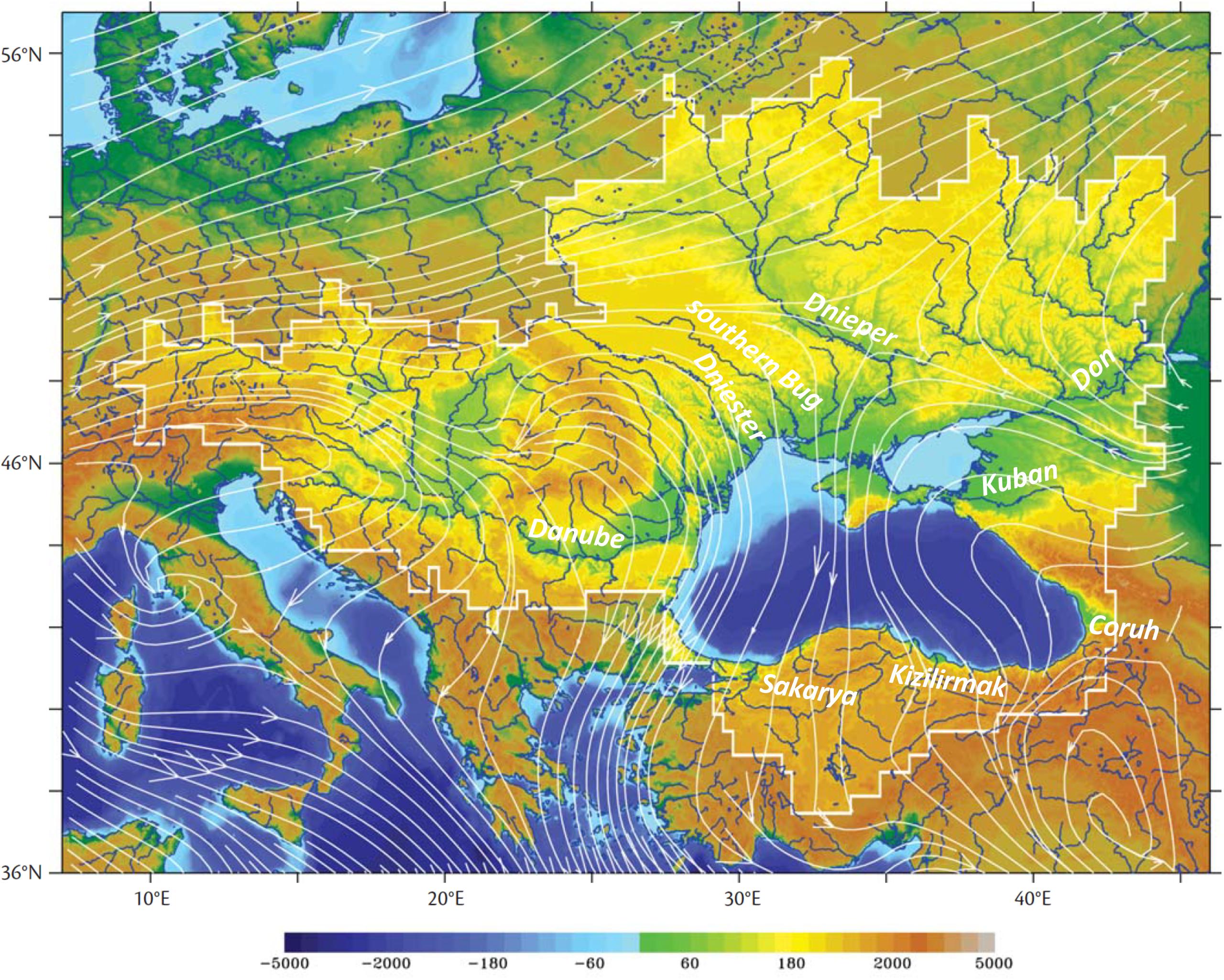
Figure 1. The Black Sea and its catchment area. The orography in the catchment area (m) is plotted with brighter colors. The streamlines illustrate the annual mean surface wind computed from ERA-40 data (replotted from Stanev, 2005).

Marine litter (ML) pollution has been observed in the Black Sea in the recent decade: on beaches (Topçu et al., 2013; Simeonova et al., 2017; Terzi and Seyhan, 2017); on the seafloor (Topçu and Oztürk, 2010; Moncheva et al., 2016; Bat et al., 2017; Öztekin and Bat, 2017); and on the sea surface (Suaria et al., 2015). Plastic objects account for a large part of the litter on various beaches in the Black Sea (Topçu et al., 2013; Simeonova et al., 2017). However, the existing information on ML quantities and distribution in the Black Sea water column, on the bottom and on the coast is still fragmented. The abundance and composition of the benthic litter on the western shelf (in the vicinity of the Bosporus Straits) have been reported by Topçu and Oztürk (2010). Ioakeimidis et al. (2014) reported that the mean FML density in the Constanta Bay was 291 ± 237 items km^–2. This high density was explained by the great influence of the Danube River; however, the density value was comparable to those at other Mediterranean coastal sites.

The recent study of Simeonova et al. (2017) provides one example of the surveys conducted on beaches along the western Black Sea coast. These surveys also identified a predominance of artificial polymer materials with densities ranging from 0.0587 ± 0.005 to 0.1343 ± 0.008 items m^–2. The pilot quantitative assessment of ML on the bottom performed by Moncheva et al. (2016) demonstrated that (1) plastic was the most common debris material found in their area of study, which was very much in line with global findings, as well as with the results of Simeonova et al. (2017), and (2) the abundance and distribution of ML showed considerable spatial variability. Understanding these phenomena calls for an in-depth examination of the methodologies for collection, classification and quantification of litter. It is stated Moncheva et al. (2016) that “a meaningful estimation of ML distribution and density could be achieved only in the context of a broader regional management framework ensuring a large-scale integrated monitoring across countries and environments (beaches, water column and sea floor) complemented by adequate understanding of the hydrodynamic features.” In this context, the identification of the main pollution sources is of prime importance.

It is not expected that in the near future, all necessary observations in time and space will be available; therefore, one could try to advance the knowledge of FML patterns using numerical modeling. Synergy between the observations and modeling results has demonstrated the potential to improve the quality of environmental assessment and predictions. Closing the gap between observational and theoretical studies presents an important motivation for the present study, which describes a theoretical framework to quantify the FML concentration in the Black Sea.

Although the circulation of the Black Sea is well known (Oğuz and Besiktepe, 1999; Korotaev et al., 2003; Zhurbas et al., 2004; Stanev, 2005), the fate of FML in the open ocean remain unclear. Objects that are denser than seawater (naturally or due to biofouling) sink and accumulate on the bottom; less dense objects float on the sea surface and are transported by currents, waves and wind; some of these floating objects are washed ashore. It is expected that areas of weak circulation act as traps for sinking ML and/or that FML accumulates in frontal areas. One of the aims of the present research is to examine these hypotheses using data from numerical models.

To date, large-scale accumulation areas similar to garbage patches (e.g., in the Hawaii region) have not yet been observed in the Black Sea. The chaotic and time-dependent character of ocean flows makes the theoretical prediction of transport difficult. Three-dimensional circulation modeling in the Black Sea reached a high level of maturity both in the field of structured-grid modeling (Stanev, 2005) and in the development of unstructured-grid models (Stanev et al., 2017), which are well fitted to the coastal regions. Presently, the research community has access to freely available products from operational models¹. These models assimilate data, which increases the credibility of these products.

Lagrangian observations in the Black Sea have been reported by Zhurbas et al. (2004). Recently, Silvestrova et al. (2016) demonstrated the usefulness of using the global positioning system to obtain high-quality positioning data over wide areas and long times. Trajectories of Argo floats in the Black Sea during the last fifteen years mostly follow the continental slope (Stanev et al., 2019b), similar to the trajectories of surface drifters reported by Zhurbas et al. (2004).

Lagrangian modeling in the Black Sea has been mostly used for predicting the transport and dispersal of oil spills. One example is the study of Korotenko (2016), who used Lagrangian tracking to analyze various scenarios of hypothetical deep-sea oil blowouts. However, to the authors’ knowledge, Lagrangian modeling has not yet been used to study FML patterns in the Black Sea and potential FML accumulation zones.

There have been a number of studies in recent decades (Moore et al., 2001; Lebreton et al., 2012; Maximenko et al., 2012; van Sebille et al., 2012, 2015) addressing the global oceanic patterns of marine debris. A recent review on Lagrangian ocean analysis by van Sebille et al. (2018) has been published. These works demonstrated the potential of numerical modeling as a guideline for assessment and management measures. One of the specific aims of the present study is to analyze the propagation of particles at the surface of the Black Sea and compare the patterns with known information from observations. The challenge is thus to start building the theoretical framework based on numerical modeling as a complement to direct and remote sensing methods of FML quantification. Another fundamental aim of the present study is to identify sensitive stretches of vulnerable shorelines affected by FML originating from rivers.

The paper is structured as follows: we first present the used data and modeling, followed by analysis of results and discussion. Short conclusions are given at the end.

The Modeling Framework

Ocean Circulation

Ocean currents for 2017 have been retrieved from the freely available Black Sea data distributed by Copernicus². The numerical model used to produce these data is based on version 3.4 of the Nucleus for European Modeling of the Ocean (Madec and the NEMO team, 2012). The model’s horizontal grid resolution is 1/36° zonally and 1/27° meridionally (ca. 3 km) and has 31 unevenly spaced vertical levels. This resolution resolves the mesoscale eddies (the Rossby radius of deformation in the Black Sea is ∼20 km). Bathymetry is based on the General Bathymetric Chart of the Oceans (GEBCO) dataset³.

The atmospheric fields used to force the model are 10-m wind, total cloud cover, 2-m air temperature, 2-m dew point temperature and mean sea level pressure. These data originate from the operational forecast of the European Centre for Medium-Range Weather Forecasts (ECMWF) at 1/8° spatial resolution and a 3-h time resolution of records. Precipitation fields over the basin are from monthly Global Precipitation Climatology Project (GPCP) rainfall data (Adler et al., 2003; Huffman et al., 2009). Bulk equations (Grayek et al., 2010), atmospheric data and current modeled sea surface temperatures are used to compute the momentum, heat and water fluxes at the air-sea interface. The monthly mean dataset provided by Ludwig et al. (2009) is used for river runoff. The boundary condition in the Bosporus Strait follows the formulation of Stanev and Beckers (1999) and Peneva et al. (2001). The model assimilates along-track sea level anomaly (SLA) and gridded sea surface temperature (SST) observations provided by Copernicus thematic assembly centers. Data assimilation uses a three-dimensional variational (3DVAR) scheme (Dobricic and Pinardi, 2008; Storto et al., 2011). Further details about the model set up are given by Ciliberti et al. (2019).

An overall presentation of surface circulation exemplified by the mean 2017 sea level (Figure 2A) demonstrates that the operational model realistically simulates the most important and well-known hydrodynamic feature, which is the general circulation gyre in the basin interior (compare with Stanev, 2005). The sea level is high on the northwest shelf and in the near-coastal areas where the circulation is overall anticyclonic. The variability pattern presented as the standard deviation of sea level from the local mean value (Figure 2B) shows the largest amplitudes in the area of the eastern Black Sea and where the Crimea eddy is usually observed. Comparison with direct altimeter observations [Ssalto/Duacs products of Archiving Validation and Interpretation of Satellite Oceanographic Data (AVISO)⁴ ] demonstrates that while the spatial simulated variability characteristics are realistic, the model overestimates the sea level oscillation amplitudes (Figure 2C). The area mean rate between the temporal variability in the altimeter data versus the model data is 0.58.

FIGURE 2

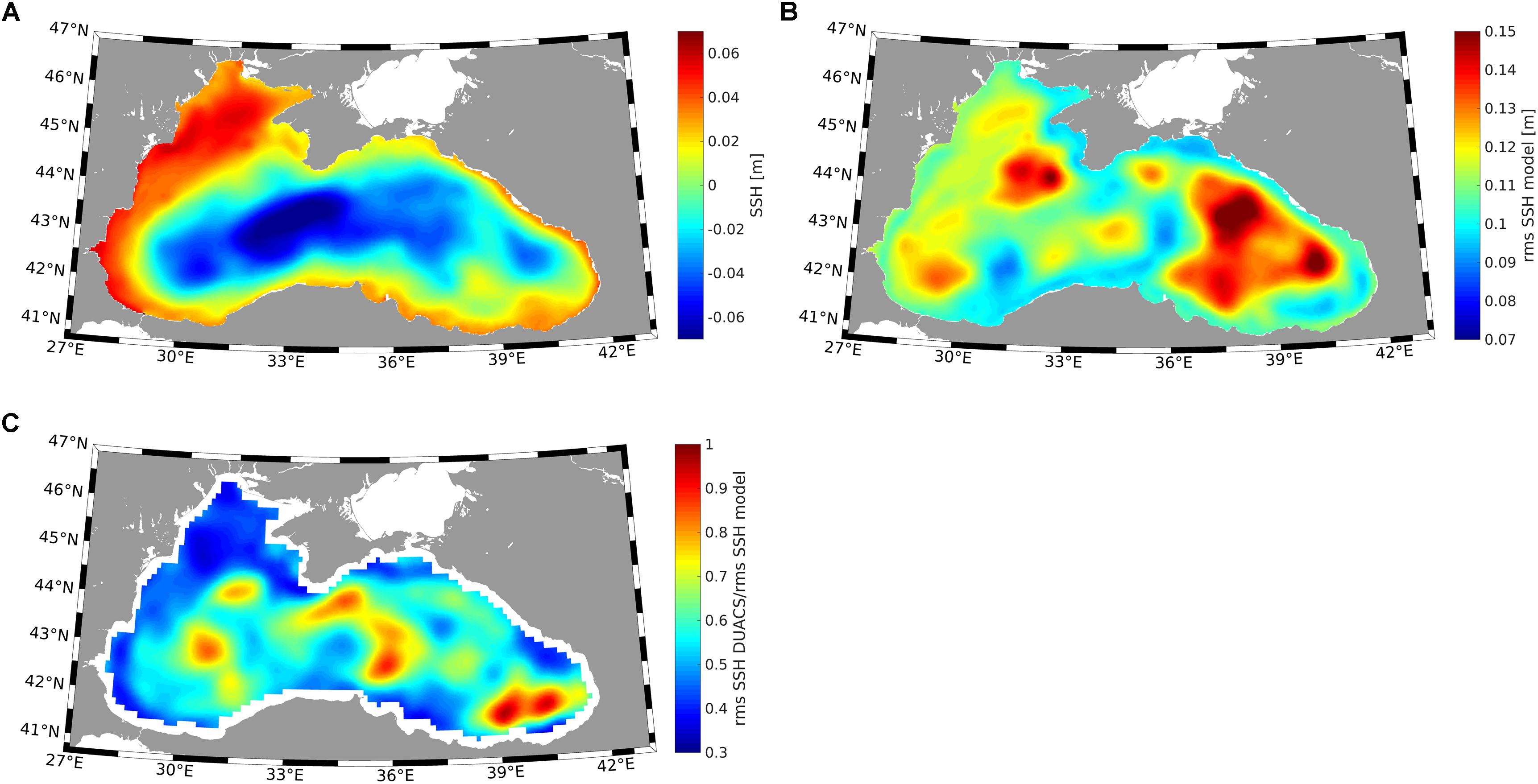
Figure 2. Annual mean sea level for 2017 from the Black Sea Copernicus product (http://marine.copernicus.eu/) (A) and its temporal variability estimated as the standard deviation of sea level from its local mean value (B). The model area does not cover the Azov Sea; therefore, results are not shown for this basin. Panel (C) shows the ratio of sea-level variability directly estimated from DUACS data and Panel (B).

Stokes Drift

The second set of operational modeling data included Stokes drift velocities. The data are produced from the third generation spectral wave model (WAM) adapted to the Black Sea area and are freely available on the Copernicus website. The model is based on the spectral description of the wave conditions in frequency and directional space. It computes the two-dimensional wave variance spectrum through integration of the transport equation in spherical coordinates.

A detailed description of WAM is given by the WAMDI Group (1988), Komen et al. (1994), Günther et al. (1992), and Janssen (2008). In WAM cycle 4.5.4, which is used for the Black Sea, the spatial grid is the same as that in the circulation mode. Twenty directional and 30 frequency bins are specified. The model considers depth refraction and wave breaking. The driving for the wave model are the same ECMWF data, which are used in the circulation model.

Additional details about operational wave modeling in the Black Sea are given by Behrens et al. (2019). In Figure 3, as an example, we show the annual mean wind and Stokes drift during 2017 and their variability patterns, estimated as $\overline{u^2+v^2}-\left({\overline{u}}^2+{\overline{v}}^2\right)$, where u and v are either wind or Stokes drift velocity and $\overline{.}$ denotes their time averaged value for the period of analysis (1 year). The annual mean wind field reflects the known horizontal pattern obtained in earlier studies (Stanev et al., 1995). The Stokes drift shows large similarity with the wind field. The largest variability associated with wind and wind waves occurs in the northern and western Black Sea.

FIGURE 3

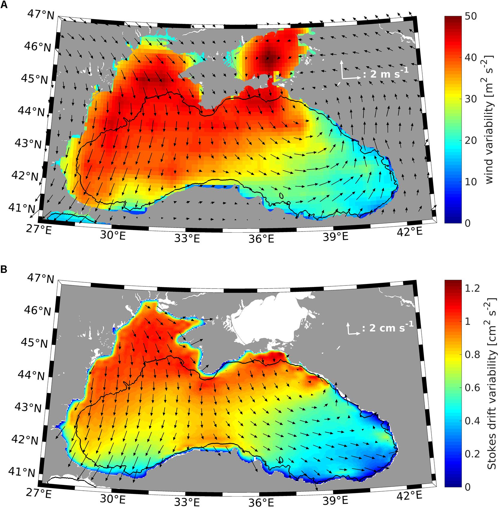
Figure 3. Annual mean for 2017 of the wind (A) and Stokes drift (B) vectors for every ∼50 km, as well as their respective spatial variability (in colors) estimated as $\overline{u^2+v^2}-\left({\overline{u}}^2+{\overline{v}}^2\right)$. The wave model does not cover the Azov Sea; therefore, results are not shown for this basin. The black lines show the 200 m isobaths.

Lagrangian Modeling

Experiments were carried out offline using the surface velocity and Stokes drift data from the Copernicus circulation and wave models, respectively. The Lagrangian model is the freely available open-source model OpenDrift (Dagestad et al., 2017), which uses a second-order Runge-Kutta method neglecting vertical velocities (it is emphasized that we simulate FML, that is, particles, which are at the surface at all times). The coefficient of horizontal diffusion is considered a function of grid size Δl:

$$A_H=c_1*\mathrm{\Delta }{l}^{\frac{4}{3}}.$$

where c₁ = 1.1 × 10^–4 m^2/3 s^–1 (Okubo, 1971; Weidemann, 1984). The respective velocities are computed by random walk displacements:

$$u^{\prime }\left(t\right)=\sqrt{\frac{2A_H}{dt}}{R}_x(t)$$

$$v^{\prime }\left(t\right)=\sqrt{\frac{2A_H}{dt}}{R}_y(t),$$

In the above equations, R_x and R_y are normally distributed random numbers with zero mean and unity variance. The time step is dt = 1 h.

Experiments

We consider FML to be Lagrangian particles. The experiments aim to (1) analyze the FML trajectories seeded uniformly across the entire basin (Experiment 1); (2) use particle tracking to simulate the trajectories of particles originating from river mouths (Experiment 2). In the first experiment, we aim to identify the possible FML clustering caused by hydrodynamics. In other words, we analyze hydrodynamics from the Lagrangian perspective. To reach this aim, a domain-wide, uniform initial distribution is prescribed with 1 particle per model grid (∼45,000 particles in total). Seeding is repeated at the beginning of each month, and tracking is performed for the twelve individual months of 2017. New seeding is performed because, after a long time (1 month), particles leave certain areas. If no new seeding occurs, these areas are emptied, and there will be no Lagrangian information for these areas. No stranding is allowed for the particles in Experiment 1.

In the second experiment, particle fluxes are prescribed in the river mouths of the eight largest rivers and in the Kerch Strait. The net transport in the Kerch Strait is taken as the sum of the river runoff from the Don and Kuban rivers. The runoff of the Dnieper and Southern Bug rivers (the mouths of which are very close to each other) are summed in one location. The major assumption in this experiment is that the concentration is the same for all rivers; that is, the amount of released particles depends only on the annual river discharge. This simplification was chosen because there are no data available for the FML concentration in individual rivers and over long periods. The release is daily and continuous in time. These particles were allowed to strand. Tracking was continued for the whole year of 2017.

It is well known that FML velocities depend not only on how drifters respond to surface waves and ocean currents but also on the direct surface drag (Daniel et al., 2002; Breivik and Allen, 2008; Röhrs et al., 2012; Stanev et al., 2019a). The relative contributions of each of these three factors are different depending on the specific drifter (e.g., percentage of its volume above the sea surface). In our simulations, the direct wind drag has been neglected, which would assume that floating objects are just below the sea surface. This simplification was introduced because there are no basin-wide data available for the size and exposure to wind of FML in the Black Sea, which is needed to determine the wind drag.

Validity of Numerical Analyses

The practices in Lagrangian ocean analysis and the associated problems and validation issues are addressed in depth by van Sebille et al. (2018). Therefore, here, we only briefly summarize some issues concerning the validity of our model results. The use of valid advection fields (currents, Stokes drift and direct surface drag) is a precondition for a credible Lagrangian simulation. In the present study, we use outputs from operational models, which assimilate altimeter and profile data and have been widely validated. Therefore, we assume that the driving data are close to the best data currently available. This is supported by the agreement between the sea level variability seen in the simulated data and derived from altimeter data (Figure 2). As stated by van Sebille et al. (2018), the accuracy of the diagnosed pathways improves by increasing the number of deployed particles. In Experiment 1, we deploy one particle per grid (model resolution, ∼3 km), which means that for a basin area of only ∼436 km³, there are ∼45,000 particles. As seen in Figure 4, the Lagrangian trajectories resolve the mesoscale motion.

FIGURE 4

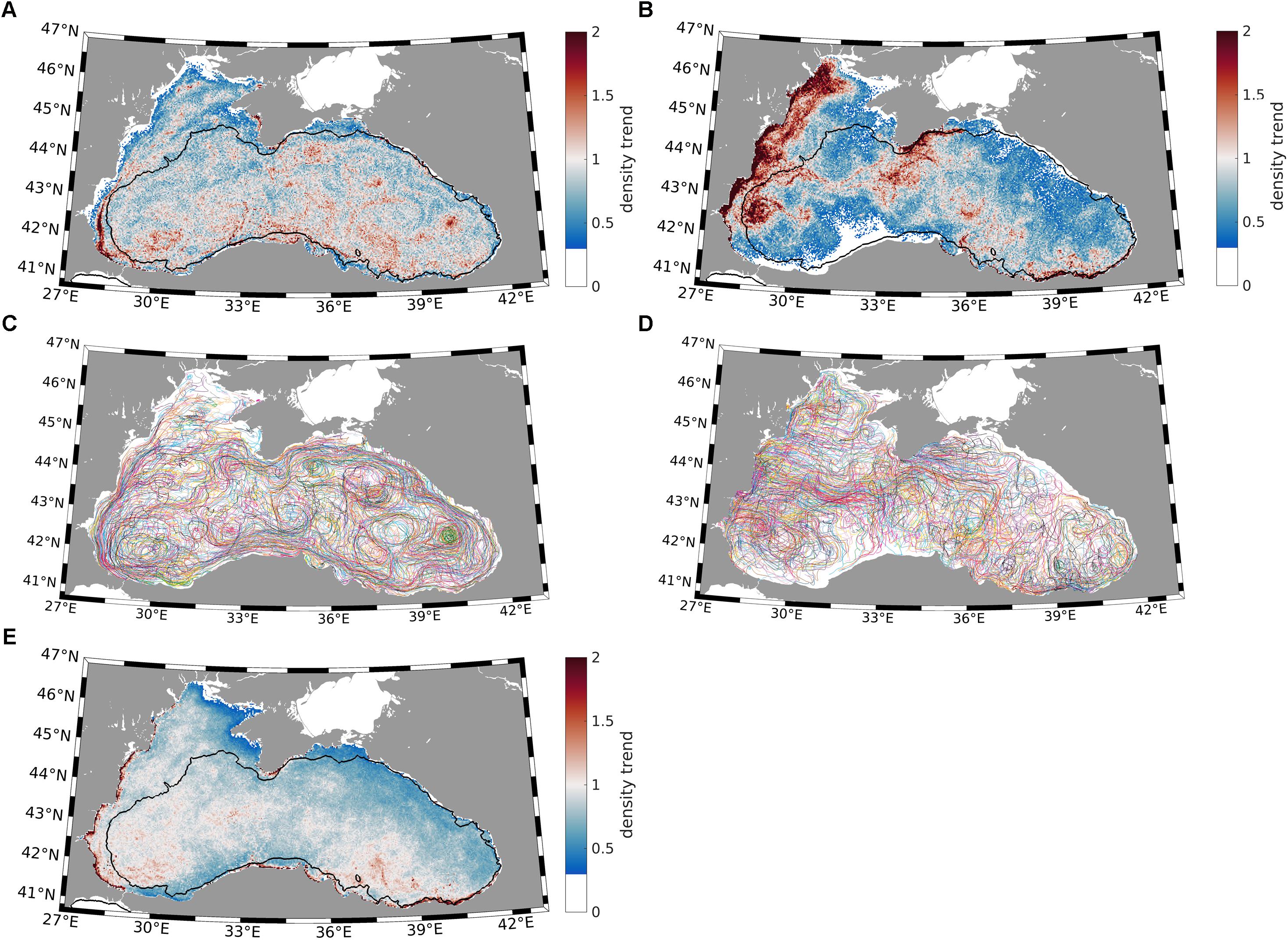
Figure 4. Density trends for January 2017 (A) and July 2017 (B) computed using surface currents only. The Lagrangian trajectories for the 2 months are shown in panels (C,D). Every 40th trajectory is shown (∼1000 trajectories in total); the colors correspond approximately to those used by van Sebille et al. (2018). Panel (E) is the monthly averaged density trend for 2017 computed as the mean trend from twelve seedings. Lagrangian tracking for each seeding was conducted for 1 month. The black line shows the 200 m isobaths.

van Sebille et al. (2018) stated that most of the available Lagrangian particle-tracking tools have never been compared with each other. Thus, the relative performance of the models is unclear; however, most of them (including the model in the present study) use at least the second-order or higher Runge-Kutta method, which ensures high accuracy.

The challenges in validation are associated with (i) the variety of object sizes and shapes; (ii) the complexity of chemical composition, decay processes and sinking of FML; and (iii) the unknown sources and sinks. There are few reliable and comparable data on FML concentration in the open ocean. As stated by Maximenko et al. (2019), estimates of the amount of microplastics floating at the sea surface reported by different authors vary between 6,350 and 236,000 metric tons (Cózar et al., 2014; Eriksen et al., 2014; van Sebille et al., 2015). One currently unresolved problem is the lack of validation data for the open Black Sea: (1) there are no drifter data for the Black Sea for the period of our analysis, and (2) there are no FML data available for the interior Black Sea [see the database of van Sebille et al. (2015)]. Therefore, the experiments described in the previous section aim at obtaining an overall geophysical consistency based primarily on the oceanographic conditions, atmospheric and river forcing. Regarding the validation of the Lagrangian model, in the present study, we use the same model used by Stanev et al. (2019a), who validated its performance against GPS-surface drifters (Meyerjurgens et al., 2019) and wooden drifters in the North Sea. The performance of the model as demonstrated by Stanev et al. (2019a) was very encouraging, in particular when simulating the stranding positions (see Figure 7 in the cited work). Therefore, we apply here the same model to the Black Sea (a basin which has similar dimensions as the North Sea), and use similar physical drivers (Copernicus data) as in our earlier study.

Results

Accumulation in the Open Ocean

FML Density Trends

The general circulation in the open sea is cyclonic. Following the general ideas developed by Stanev et al. (2000, 2004), the Ekman drift tends to displace surface water from the interior into the coastal zone, and the water deficit in the basin interior is compensated by a general upwelling. This situation would suggest that FML would tend to leave the basin interior and move toward coasts.

To evaluate this hypothesis, we use the results from Experiment 1. After each month of Lagrangian integration, we compute the particle density trend (DT). The particle DT reflects the number of particles that have visited each grid cell during a certain time interval. (See Koszalka and LaCasce (2010) and Huntley et al. (2015) for more details about the used clustering metrics.) This quantity is normalized by the respective number, which corresponds to a motionless situation for the same time interval, in our case 1 particle per grid cell:

$$DT(x,y,t_n)=\frac{{\sum }_{i=0}^n{N}_{u\ne 0}(x,y,t_i)}{{\sum }_{i=0}^n{N}_{u=0}(x,y,t_i)}$$

In the above equation, (x, y) are the coordinates of an arbitrary grid cell with size (dx, dy), n are the time steps from t₀ to t_n, u is the velocity field and N is the number of particles at time step i in grid (x, y). In the present study, (dx, dy) is the model grid size; (dx, dy) can be prescribed larger or smaller than the model grid size depending on the application. A DT larger/smaller than unity corresponds to more/less particles that have been identified in a grid cell on average than there would have been without currents. Thus, the DT can be interpreted as the percentage of the initial particle amount averaged over time. The DT transforms the Lagrangian characteristics into the so-called pseudo-Eulerian property that is similar to the density, which represents the process of particle compaction in certain areas. In this way, one can identify particle accumulation areas. This approach is similar to the technique of binning particle positions into histograms (Koszalka et al., 2011). One can also generate probability maps (e.g., van Sebille et al., 2012; von Appen et al., 2014; van Sebille et al., 2018).

If the number of particles in some areas remains small (see the January and July trends in Figures 4A,B, respectively), statistical confidence of the DT is not ensured. Therefore, the areas where the DT is smaller than 30% are excluded from the analysis (white areas). This result explains the reasons to divide Lagrangian tracking into several seeding runs (in this case, t_n is chosen to be 1 month).

Accumulation Patterns Caused by Currents

The large variability of circulation patterns explains the difference between the DTs in individual months. While the distribution of the accumulation patterns in January is characterized by an overall trend of increasing concentrations to the southern areas and decreasing concentrations in the northern areas (Figure 4A), the July pattern (Figure 4B) clearly demonstrates a very strong accumulation along the western coasts and in the area south of Crimea. In both cases, the DT reveals compaction areas, which are reminiscent of eddy and subbasin eddy features and filaments (compare with Figures 4C,D).

Averaging the monthly DTs over a year decreases the horizontal FML gradients. The overall conclusion from the annual mean pattern (Figure 4E) is that the concentrations decrease in the eastern and northern areas and increase along the western coasts. The former is a result of the dominant northerlies (Figure 3A), which impact the current in the surface layer. Similar trends in the Black Sea were recently reported by van Sebille et al. (2015) from global simulations covering the area of the Black Sea. Because of the very different resolutions used in the regional and global models, we do not speculate further on these agreements. Noteworthy is that at the global level, the Black Sea, along with the Mediterranean, shows the largest concentrations of particles.

Accumulation Patterns Caused by Currents and Stokes Drift

Adding Stokes drift to the surface current has non-trivial consequences, although the pattern of Stokes drift is relatively smooth. In January (compare Figures 5A to 4A), Stokes drift resulted in south-eastward FML displacements, which is well seen along the eastern coast. The DT in the presence of Stokes drift appears slightly smoother, with the exception of the area to the south of the Kerch Strait, where the joint effect of surface currents and Stokes drift resulted in an accumulation zone with complex spatial characteristics.

FIGURE 5

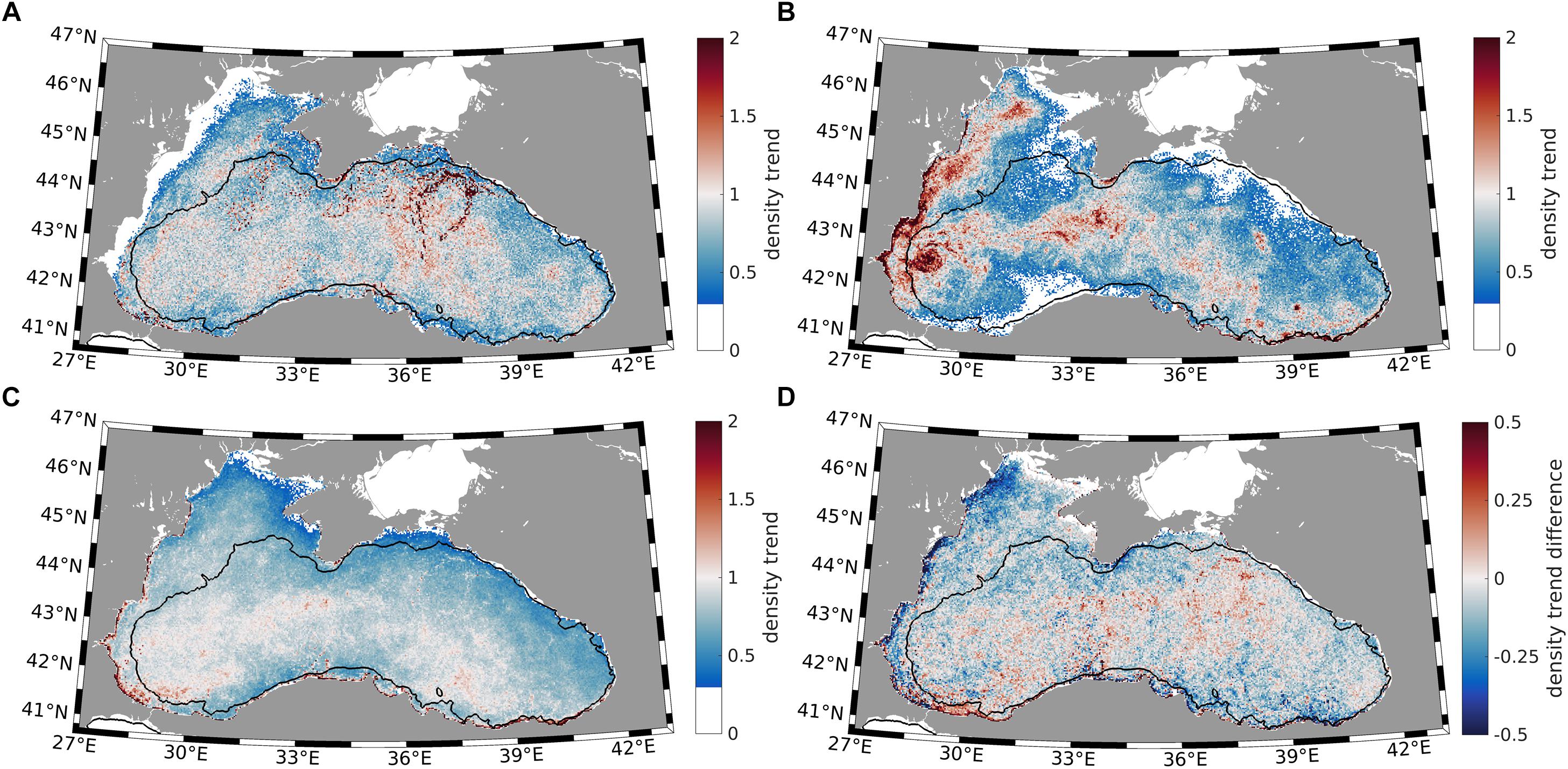
Figure 5. Panels (A–C) shows the same as Figures 4A–C, but Stokes drift has been added. (D) shows the contribution of Stokes drift for 2017, which is the difference between panel (C) and Figure 4E. Note the different contour interval in panel (D). The black lines show the 200 m isobaths.

There are also no large changes in the DTs in July caused by Stokes drift (compare Figures 5B to 4B). Overall, the wave effects resulted in a slight decrease in FML accumulation along the western coasts. The changes are even smaller if one considers the annual mean situation (compare Figures 5C and 4E). The net contribution of waves results in greater FML accumulation in the southwestern Black Sea and less accumulation on the North-West shelf (Figure 5D). Note that the contour interval of Figure 5D is four times smaller than those of the remaining plots. The consistency in FML accumulation between the region along the southern coast and Figure 3B suggests a clear linkage to the Stokes drift pattern. These results support other recent estimations revealing the important impact of Stokes drift on the movement of surface drifters in the North Sea (Stanev et al., 2019a) and the fate of FML in the South Indian Ocean (Dobler et al., 2019). In a study on the global accumulation of floating microplastics, Onink et al. (2019) showed that Stokes drift tends to enhance microplastic transport to the Arctic Ocean.

Accumulation on Coasts

In the experiment aimed at quantifying FML propagation from rivers and its stranding (Experiment 2), particles are propagated by the surface current and Stokes drift. Particles from each river are colored in Figure 6 with different colors. Because the FML flux at the river mouth is considered proportional to the water flux only, most of the particles originate from the Danube, which is the major source of fresh water. The FML distribution in the open sea shows areas of increased concentrations, some of which have eddy scales. This is a clear illustration of clustering. The patterns in Figure 6, ∼4 and 5 months after the start of integration, are short-lived patterns. They change with the time scale, which is characteristic of the synoptic atmospheric variability. Overall, the preferred stranding positions are determined by the cyclonic character of circulation, that is, particles strand to the right of the river mouth looking in the direction of the sea. One exception is the area of the Batumi (anticyclonic) eddy, where particles from the Coruh River turn to the left.

FIGURE 6

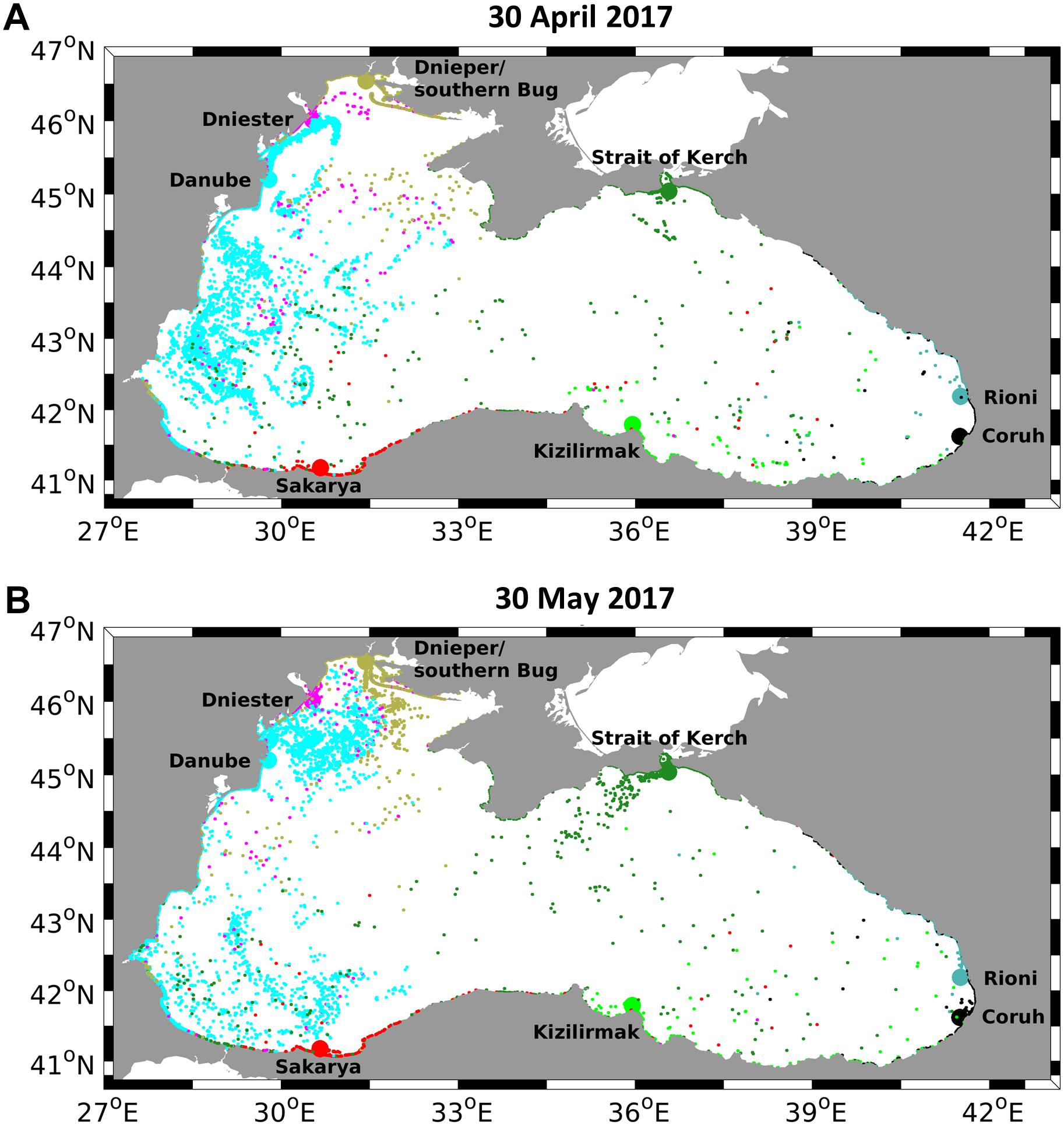
Figure 6. Example distribution of the floating objects (small dots) from rivers (large dots show their mouths) under different weather conditions: after 4 months of Lagrangian tracking on 30 April 2017 (A) and 1 month later, on 30 May 2017 (B). Notice that the number of particles in the open ocean does not considerably increase because of stranding. For particle advection, surface velocities and Stokes drift data were used.

Figure 7A shows the temporal evolution of floating particles in Experiment 2 integrated over the entire basin. The number of particles continuously increased after the start of the experiment. The maximum number was reached at approximately seven months and was ∼4–5 times lower than the number of released particles (Figure 7C). This result indicates that most of the released particles stranded. In the period August-November, most of the floating particles were washed ashore, and the total amount decreased extensively. An increasing trend was initiated at the end of 2017.

FIGURE 7

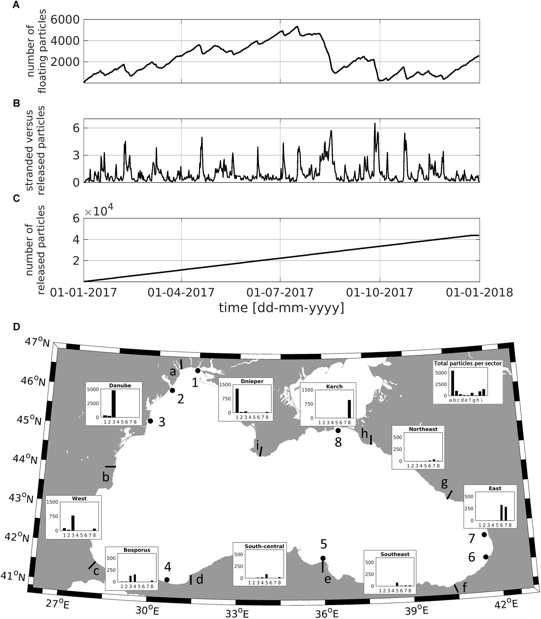
Figure 7. Temporal evolution of the number of floating particles (A), the ratio of the current number of stranded particles to the number of released particles (B) and the total number of released particles (C) in Experiment 2. (D) shows the number of stranded particles released from rivers after 1 year of integration within the respective coastal sectors (letters). The bars and the letters next to the bars show the start and end positions of the individual sectors, respectively. These sectors are also named in the insets; for instance, the first sector, a-b, is called Danube, and the last sector, i-a, is called Dnieper. The numbers in this figure next to the circles correspond to individual rivers and the Kerch Strait. The insets show the accumulated FML amounts in the respective sectors. Note that the different bar widths and the different maxima of the vertical axes illustrate very different accumulation trends on the coasts. For particle advection, surface velocities and Stokes drift data were used.

The numbers in Figure 7A can be considered as relative ones, reflecting the prescribed fluxes. Our experiments showed that doubling the flux approximately doubles the number of FML particles. It is more objective to analyze the ratio of the current number of stranded particles to the number of released particles (Figure 7B). This number (mean value of 0.99) is highly variable, reaching values of up to 7. This unexpected result can be explained by the following scaling considerations. The ratio of the annual mean number of floating particles (2205) to the mean flux of stranded particles (113 day^–1) yields for the characteristic stranding time ∼20 days. This time is comparable to the synoptic time of atmospheric variability and is too short to allow the propagation of particles far from the coasts without being washed ashore. Because the scales of Black Sea are small, stranding times dominate the dynamics of FML and makes the consolidation of FML in large patches, as is observed in the open ocean, impossible in the basin interior. The characteristic stranding time is short not only because of the specific dynamics but also because of the prescribed stranding mechanism: we assumed that all particles that reach the coast strand, which is the upper bound of the stranding parameterization.

The following analysis aims to quantify the distribution of stranded particles along the coast. We divide the coast into ten sections. The start and end positions are illustrated in Figure 7 with bars, next to which letters allow us to distinguish between individual sectors in the following text. These sectors are also named, for instance, the first sector, a-b, is called Danube, and the last sector, i-a, is called Dnieper. The sectors are defined such that their lengths are almost the same, which enables a better comparison between their stranding properties. The numbers on this figure correspond to individual rivers. The positions of their mouths are shown with large circle symbols; their names are shown in Figure 7. There are no dependencies between the sector names and rivers; there can be more than one river in a sector or no rivers.

The quantification of stranding is visualized in the insets showing the amount of FML particles from each river identified in the individual coastal sectors. Most of the stranding particles originate from the Danube, which explains the large amount of stranded particles in sector a-b, Danube. The vertical axes in the individual sectors are chosen to be different (0–5000 for the Danube sector, 0–1500 for the West, Kerch and Dnieper sectors and 0–750 for the rest of the sectors). This system was needed to illustrate the origin of particles in areas with very different sources and accumulation properties. Overall, the most polluted are the sectors starting from the Kerch to the West sector, as well as the East region. These findings nicely reflect the close correlation between local sources, as well as sources upstream of the major Black Sea current (the Rim current), and stranded particles.

Discussion

FML propagation, accumulation and stranding predictions pose a challenge both in the observational field and in the field of their numerical modeling. Predictions and environmental estimates require reliable and comparable data. This condition necessitates standardized protocols for sampling and analysis. Performing large-scale measurements, increasing the coverage of survey sites, and developing clear ideas based on observations of the accumulation patterns in individual ocean basins and river plumes are of utmost importance to close the gap between observational and modeling approaches. For modeling, the availability of validation data is crucial. The agreement between the simulated stranding results on the western Black Sea coast and available observations is a good first step toward validation of model estimates. Furthermore, one could expect that numerical modeling will provide theoretical evidence to be used to support or guide appropriate observations and comparisons between observations and modeling.

Moncheva et al. (2016) demonstrated that the average ML quantity in the northwestern Black Sea was an order of magnitude higher than the amounts observed in the western Black Sea. Furthermore, the ML distribution was characterized by considerable spatial variability. The respective concentrations showed a maximum in front of the Romanian coast and decreased from north to south, and the concentration was ∼3 times lower in front of the Bulgarian coast (9598 items km^–2). This decrease continued further south; the item concentration encountered in front of the Turkish coast was 7956 items km^–2. These results provide good support for our modeling. The decrease in concentration from coastal areas to the open ocean also supports the results of Experiment 2. As Moncheva et al. (2016) stated, coastward along the 40 m isobath, the abundance of ML was generally much higher than on the continental shelf (see also Figure 4E).

Our simulations did not reveal similarities to known cases from other ocean areas of FML compaction, e.g., the Great Pacific Garbage Patch. The results shown in Figures 4, 5 also do not reveal a strong consistency with known circulation patterns in the Black Sea (Figure 2A) over long time periods. The short stranding time quantified in section “Accumulation on Coasts” partially explains the difference in cluster formation between small (semi-enclosed) basins and the open ocean. In the following, additional reasons for the observed distribution of FML are given. Figure 8A shows the trajectories of FML originating from coastal regions shallower than 200 m computed in Experiment 1 twenty days after the release on 1 January 2017. Most of the particles originate from the northwest shelf. The contribution from the remaining coastal areas of the Black Sea is small because the 200 m isobaths there are very close to the coast, in particular along the eastern coast. The intrusions into the open sea are dominated by mesoscale eddies and meanders of the Rim current. This propagation pattern is consistent with the known role of mesoscale eddies. (Notice the recirculating wakes structures formed behind coastal headlands, particularly along the southern coast.) Shelf break eddies substantially contribute to cross-shelf exchange (Shapiro et al., 2010), creating filaments that intrude into the basin interior. The Lagrangian trajectories simulated in Experiment 1 evidence the role of these filaments in the propagation of FML and support the conclusion in section “Accumulation on Coasts” that clustering in the Black Sea appears only over short time scales.

FIGURE 8

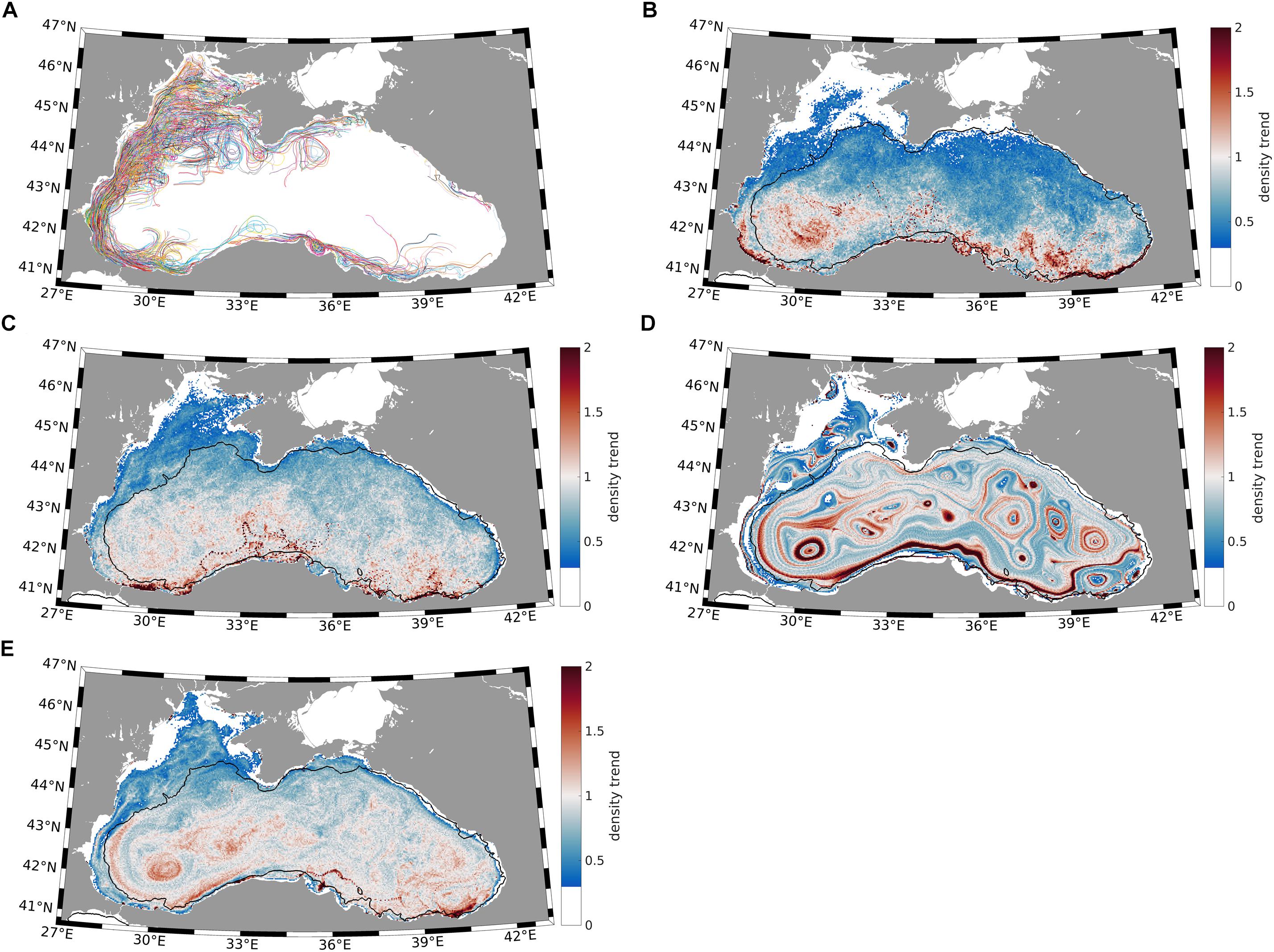
Figure 8. Trajectories of particles in Experiment 1 released in areas shallower than 200 m (thick black isobaths) from 1 to 20 January 2017 (A). Every 10th trajectory is shown; colors correspond to those in Figure 4. DT from January to June 2017 in Experiment 1 (B). DT computed using non-stationary geostrophic surface currents for the period from January to June 2017 (C). DT from January to June 2017 computed using geostrophic surface currents obtained from the mean January to June sea level values (D). DT from January to June 2017 computed using non-geostrophic surface currents with a reduced (three times) range of the temporal variability (E). The black lines show the 200 m isobaths.

Analysis of the results from Experiment 1 in the previous section was targeted toward illustrating the impacts of circulation and Stokes drift on the DT. Seeding was performed every month, and the mean of the twelve one-month DTs is shown in Figures 4E, 5C. Now, we analyze only the particles released in January 2017 but track these particles for 1 year. As shown in Figure 8B, these particles exhibit a tendency to accumulate in the southern Black Sea. Six months after seeding, part of the northern Black Sea becomes free of FML. After 1 year of Lagrangian tracking, most of the northern part of the Black Sea becomes free of FML (not shown here), which is explained by the predominant Ekman and Stokes drift directions.

To isolate the roles of Ekman and Stokes drift, we computed surface velocities from current sea levels using geostrophic formulas and repeated Experiment 1. In the following, we refer to this experiment as Experiment 1_gns, where “gns” stands for geostrophic-non-stationary. The results from this experiment, which are shown in Figure 8C, did not appear principally different from the results shown in Figure 8B. This finding suggests that the pattern shown in Figure 8B is largely explained by sea level dynamics. Ekman and Stokes drift contribute to the southward displacement of FML.

Theoretically, geostrophic motion is stationary and rectilinear; although Experiment 1_gns uses geostrophic equations to derive surface velocities, the flow is ageostrophic because of the complex shape (Figure 2A) and non-stationarity (Figure 2B) of the sea level. As a next step, we used the annual mean sea surface (Figure 2A) to compute the geostrophic surface velocity and repeated the computations (Experiment 1_g) with a stationary geostrophic flow. Figure 8D shows a good consistency with the sea level pattern in Figure 2A, demonstrating that current shears and mesoscale features determine the FML pattern, revealing their clear clustering signatures. The accumulation along the front in the southern Black Sea is very pronounced and consistent with the observed accumulation of floating matter in frontal areas. The results of our experiments support the statement of Jacobs et al. (2016) that “ageostrophic ocean processes such as frontogenesis, submesoscale mixed-layer instabilities, shelf break fronts, and topographic interactions on the continental shelf produce surface-divergent flows that affect buoyant material over time”. Thus, the spatially variable sea level slope (Figure 2A), which is essentially an ageostrophic feature, explains the clustering in Figure 8D.

The major difference between Experiment 1_g and Experiment 1_gns is the non-stationarity of the velocity field (non-stationarity is also an ageostrophic signal). Clearly, this ageostrophic component of ocean currents is the major reason explaining the absence of clustering in Experiment 1_gns. Therefore, we can conclude that not all ageostrophic ocean processes lead to clustering. Unlike the case analyzed by Jacobs et al. (2016), the temporal variability of ageostrophic motion is too strong for the periods considered in our case and acts as a mixing mechanism. In other words, the ratio of the range of the sea level slope to the range of its temporal variability (the latter is estimated as the standard deviation of sea level from its local mean value) determines whether FML will compact and show pronounced hydrodynamic-like patterns. As seen from the comparison between Figures 2A,B, the range of the horizontal differences of the sea level is comparable to the range of its temporal variability.

The higher temporal variability rates in the Copernicus product compared with the variability in the altimeter data (Figure 2C) suggests that the Copernicus product overestimates the temporal variability. The rather chaotic stirring is thus caused by the strong temporal variability in Experiment 1_gns and results in a disappearance of pronounced accumulation areas.

In the next experiment, we reduced the ageostrophic variability three times (Experiment 1_gns/3) and repeated the computations to investigate whether clustering appears in the case of a lower variability range. This reduction was larger than the overestimation of the variability range in the Copernicus product. However, despite this large decrease in the variability rate, which is now lower than that in the altimeter data, most of the frontal and eddy-like patterns in Figure 8D disappeared, as shown in Figure 8E. The conclusion is that specific circulation features in the Black Sea (i.e., the divergent general circulation in the basin interior and the strong temporal variability of flow) are not favorable for FML accumulation in the basin interior over monthly and longer periods.

Under the assumption that all particles that reach the coast strand, the estimated stranding times are short. This suggests that the dynamics of FML are strongly dominated by stranding processes, which cause their concentrations in the open sea to remain low. If the FML fluxes are turned off, almost all FML will strand within ∼2 months (stranding time of 20 days). This is good news relative to the case of the global ocean, where large amounts of particles can accumulate far from the coasts and thus be difficult to clean. Thus, the coasts of semi-enclosed seas act as accumulation areas, which might potentially facilitate efforts to efficiently clean the marine environment. The above conclusions can be tested and/or generalized to other coastal and estuarine environments. The caveat is that the stranding times estimated here are the shortest possible (as all particles that reach the coast strand). This assumption can be relaxed in future studies. Determining the ratio of the concentration of FML in the open ocean to the total flux from rivers (if credible measurements exist) could facilitate the development of improved stranding parameterizations.

Further improvement of the model predictions would also necessitate a more specific and clear understanding of the sources and types of ML from individual rivers. Another step aimed at increasing the realism of the estimates would be to prescribe how much litter leaves through the Bosporus. Different sizes, classes, and categories (including nanoplastics), along with their transformations, also need to be addressed. Here, coupling with biogeochemical models is needed to account for the persistence of ML and their biodegradation.

Even with the simplifications assumed here, ML modeling gives further motivation to address transboundary problems. Our findings support the results of Topçu et al. (2013), claiming that the southeastern side of the Black Sea was found to be cleaner than the western side. According to these authors, half of the labeled ML recovered from the southwestern Black Sea (Turkey) was of foreign origin. This phenomenon represents an additional challenge for modelers to focus on coastal areas, where ML transport mechanisms and stranding are more complex. In the present simulations, the dynamics of stranding were accounted for in a very simple way: once ML hits the coast, it remains there. Clearly, this process does not consider regional coastal characteristics, which requires further attention. Using unstructured-grid models (Stanev et al., 2017), which are characterized by a higher spatial resolution and therefore fit coastal regions well, could help a lot. Such models can more accurately simulate small-scale convergence and divergence zones, notably in coastal canyons or sea mounts.

It appears that the regional case of the Black Sea analyzed here has much in common with the ideas behind the future integrated marine debris observing system (IMDOS, Maximenko et al., 2019; see also Galgani et al., 2019). This system is required to provide long-term monitoring and support operational activities associated with anthropogenic pollution. The present study reveals issues specific to regional and semi-enclosed basins and can motivate addressing with more weight the coastal and regional ocean basins in the context of the IMDOS. As in the European Copernicus program, one should start to develop regional and coastal observing and forecasting systems based on the amalgamation of observations and numerical modeling. Numerical models are useful for improving our understanding the processes that affect transport, fate and distribution of marine debris. They can be considered as complementary tools to guide observational practices using observing system experiments (OSEs) or Observing System Simulation Experiments (OSSEs). One challenge is collecting in situ observations and sensing the environment remotely to increase the amount and quality of data (Zielinski et al., 2009; Garaba et al., 2018). We thus hope that numerical modeling will be soon used for practical purposes after addressing some of the above challenges and used in support of observational activities and the development of future reduction measures and mitigation strategies. However, it is necessary to adequately address the applicability of the model data used for particle tracking. As seen from our results, the expectation that the interior of the Black Sea will transport ML into the region of the Rim current and that ML will accumulate along the Rim current was not realized except in the unrealistic case shown in Figure 8D. In the present study, we used outputs from operational models, with the assumption that the data is close to the best available data at the moment. One next step could be testing the concepts of accumulation using other available models to address FML clustering in the deep sea in a more complete way.

Conclusion

The present work is a step toward building a framework based on numerical modeling to (1) identify FML accumulation patterns in the Black Sea and (2) the vulnerable coasts affected by the FML from rivers. To reach this aim, we used freely available ocean current and Stokes drift data from Copernicus products and performed Lagrangian simulations.

At long time scales, months to a year, no pronounced FML accumulation zones and horizontal gradients were observed, and no features similar to the Great Pacific Garbage Patch were found. Overall, the FML concentrations decreased in the eastern and northern areas and increased along the western coasts. This phenomenon is due to the dominant northerlies and the resulting Ekman and Stokes drift. Even in the absence of wind effects, that is, when Lagrangian particles were driven by only geostrophic currents, FML clustering was not pronounced. This finding was explained by the non-stationarity of the velocity field. In a sensitivity experiment where surface geostrophic currents were computed from the annual mean sea level, FML clustering did appear, in particular in areas with pronounced ageostrophic ocean features such as eddies, jets and fronts. A more in-depth analysis of the currents and the resulting FML accumulation patterns demonstrated that their temporal variability was too high, which acted as a mixing mechanism. This high level of variability, which was relatively uniformly distributed across the entire sea, was prohibitive for FML compaction in specific hydrodynamic areas. In another sensitivity experiment, when the temporal variability was reduced below the level of the natural variability, traces of FML clustering started to appear. The conclusion is that the ratio between the circulation intensity (measured by the sea level slope) and the rate of its temporal variability determines whether FML will compact.

In a second experiment, addressing FML spreading from rivers and its stranding, it was found that the stranding time scales (∼20 days) were comparable to the synoptic scales in the atmosphere. This provided an explanation of the dominant short-time variability of the total number of FML particles and their low concentrations in the open ocean. The predominant stranding locations were determined by the cyclonic character of circulation. A close correlation was found between the FML quantity on coasts and the distance from the river mouths upstream of the Rim current. The simulated distribution of stranded objects was supported by available coastal and near-coastal observations. It was shown that the areas that were the most at risk extend from the Kerch Strait to the western coast. The model can be further developed by including more realistic fluxes from rivers with the aim of adequately addressing the transboundary propagation of pollution.

Data Availability Statement

The datasets generated for this study are available upon request from the authors.

Author Contributions

All authors listed have made a substantial, direct and intellectual contribution to the work, and approved it for publication.

Funding

This work was initiated as a contribution of ES to the conference “Inter-basin cooperation on marine litter; a focus on the Danube River and the Black Sea” held on 4 April 2019 in Sofia, Bulgaria. Data from the CMEMS portal for the Black Sea have been used. MR acknowledges support from the project “Macroplastics Pollution in the Southern North Sea – Sources, Pathways and Abatement Strategies” (grant no. ZN3176), which was provided by the Ministry of Science and Culture of the German Federal State of Lower Saxony.

Conflict of Interest

The authors declare that the research was conducted in the absence of any commercial or financial relationships that could be construed as a potential conflict of interest.

Footnotes

1. ^ http://marine.copernicus.eu/services-portfolio/access-to-products/
2. ^ http://marine.copernicus.eu/
3. ^ www.gebco.net
4. ^ https://www.aviso.altimetry.fr/en/home.html

References

Addamo, A. M., Brosich, A., Chaves, M. D. M., Giorgetti, A., Hanke, G., Molina, E., et al. (2018). Marine Litter Database: Lessons Learned in Compiling the First Pan-European Beach Litter Database, EUR 29469 EN. Luxembourg: Publications Office of the European Union.

Google Scholar

Adler, R. F., Huffman, G. J., Chang, A., Ferraro, R., Xie, P., Janowiak, J., et al. (2003). The version 2 global precipitation climatology project (GPCP) monthly precipitation analysis (1979-Present). J. Hydrometeor. 4, 1147–1167. doi: 10.1175/1525-7541(2003)004<1147:tvgpcp>2.0.co;2

CrossRef Full Text | Google Scholar

Barnes, D. K. A., Galgani, F., Thompson, R. C., and Barlaz, M. (2009). Accumulation and fragmentation of plastic debris in global environments. Philos. Trans. R. Soc. 364, 1985–1998. doi: 10.1098/rstb.2008.0205

PubMed Abstract | CrossRef Full Text | Google Scholar

Bat, L., Öztekin, A., and Arıcı, E. (2017). “Marine litter pollution in the black sea: assessment of the current situation in light of the marine strategy framework directive,” in Black Sea Marine Environment: The Turkish Shelf, eds M. Sezgin, L. Bat, D. Ürkmez, E. Arıcı, and B. Öztürk (Istanbul: Turkish Marine Research Foundation).

Google Scholar

Behrens, A., Staneva, J., Krueger, O., and Lecci, R. (2019). User Manual for Black Sea Waves Reanalysis Product. Available at: http://resources.marine.copernicus.eu/documents/PUM/CMEMS-BS-PUM-007-006.pdf (accessed October 15, 2019).

Google Scholar

Breivik, O., and Allen, A. A. (2008). An operational search and rescue model for the Norwegian Sea and the North Sea. J. Mar. Syst. 69, 99–113. doi: 10.1016/j.jmarsys.2007.02.010

CrossRef Full Text | Google Scholar

Ciliberti, S., Lecci, R., Creti, S., Lemieux-Dudon, B., Lima, L., Storto, A., et al. (2019). User manual for the Black Sea Physics Analysis and Forecast Product. Available at: http://resources.marine.copernicus.eu/documents/PUM/CMEMS-BS-PUM-007-001.pdf (accessed October 15, 2019).

Google Scholar

Cózar, A., Echevarría, F., González-Gordillo, I., Irigoien, X., Úbeda, B., Hernández-León, S., et al. (2014). Plastic debris in the open ocean. Proc. Natl. Acad. Sci. U.S.A. 111, 10239–10244. doi: 10.1073/pnas.1314705111

PubMed Abstract | CrossRef Full Text | Google Scholar

Dagestad, K.-F., Röhrs, J., Breivik, Ø, and Adlandsvik, B. (2017). OpenDrift v1.0: a generic framework for trajectory modeling. Geosci. Model Dev. Discuss. 11, 1405–1420. doi: 10.5194/gmd-2017-2205

CrossRef Full Text | Google Scholar

Daniel, P., Jan, G., Cabioc’h, F., Landau, Y., and Loiseau, E. (2002). Drift modeling of cargo containers. Spill Sci. Technol. Bull. 7, 279–288. doi: 10.1016/S1353-2561(02)00075-0

CrossRef Full Text | Google Scholar

Dobler, D., Huck, T., Maes, C., Grima, N., Blanke, B., Martinez, E., et al. (2019). Large impact of Stokes drift on the fate of surface floating debris in the South Indian Basin. Mar. Pollut. Bull. 148, 202–209. doi: 10.1016/j.marpolbul.2019.07.057

PubMed Abstract | CrossRef Full Text | Google Scholar

Dobricic, S., and Pinardi, N. (2008). An oceanographic three-dimensional assimilation scheme. Ocean Modell. 22, 89–105. doi: 10.1016/j.ocemod.2008.01.004

CrossRef Full Text | Google Scholar

Eriksen, M., Lebreton, L., Carson, H., Thiel, M., Moore, C., Borerro, J., et al. (2014). Plastic pollution in the World’s oceans: more than 5 trillion plastic pieces weighing over 250,000 Tons Afloat at sea. PLoS One 9:e111913. doi: 10.1371/journal.pone.0111913

PubMed Abstract | CrossRef Full Text | Google Scholar

Garaba, S. P., Aitken, J., Slat, B., Dierssen, H. M., Lebreton, L., Zielinski, O., et al. (2018). Sensing ocean plastics with an airborne hyperspectral shortwave infrared imager. Environ. Sci. Technol. 52, 11699–11707. doi: 10.1021/acs.est.8b02855

PubMed Abstract | CrossRef Full Text | Google Scholar

Grayek, S., Stanev, E., and Kandilarov, R. (2010). On the response of Black Sea level to external forcing: altimeter data and numerical modelling. Ocean Dyn. 60, 123–140. doi: 10.1007/s10236-009-0249-7

CrossRef Full Text | Google Scholar

Günther, H., Hasselmann, S., and Janssen, P. A. E. M. (1992). The WAM Model Cycle 4.0. User Manual. Technical Report No. 4. Hamburg: Deutsches Klimarechenzentrum, 102.

Google Scholar

Huffman, G. J., Adler, R. F., Bolvin, D. T., and Gu, G. (2009). Improving the global precipitation record: GPCP version 2.1. Geophys. Res. Lett. 36:L17808. doi: 10.1029/2009GL040000

CrossRef Full Text | Google Scholar

Huntley, H. S., Lipphardt, B. L. Jr., Jacobs, G., and Kirwan, A. D. (2015). Clusters, deformation, and dilation: diagnostics for material accumulation regions. J. Geophys. Res. Oceans 120, 6622–6636. doi: 10.1002/2015JC011036

CrossRef Full Text | Google Scholar

Ioakeimidis, C., Zeria, C., Kaberia, H., Galatchic, M., Antoniadisd, K., Streftarisa, N., et al. (2014). A comparative study of marine litter on the seafloor of coastal areas in the Eastern Mediterraneann and Black Seas. Mar. Pollut. Bull. 89, 296–304. doi: 10.1016/j.marpolbul.2014.09.044

PubMed Abstract | CrossRef Full Text | Google Scholar

Jacobs, G. A., Huntley, H. S., Kirwan, A. D., Lipphardt, B. L., Campbell, T., Smith, T., et al. (2016). Ocean processes underlying surface clustering. J. Geophys. Res. Oceans 121, 180–197. doi: 10.1002/2015JC011140

CrossRef Full Text | Google Scholar

Jambeck, J. R., Geyer, R., Wilcox, C., Siegler, T. R., Perryman, M., Andrady, A. L., et al. (2015). Plastic waste inputs from land into the ocean. Science 347, 768–771. doi: 10.1126/science.1260352

PubMed Abstract | CrossRef Full Text | Google Scholar

Janssen, P. A. E. M. (2008). Progress in ocean wave forecasting. J. Comput. Phys. 227, 3572–3594. doi: 10.1016/j.jcp.2007.04.029

CrossRef Full Text | Google Scholar

Komen, G. J., Cavaleri, L., Donelan, M., Hasselmann, K., Hasselmann, S., and Janssen, P. A. E. M. (1994). Dynamics and Modelling of Ocean Waves. Cambridge: Cambridge University Press.

Google Scholar

Korotenko, K. A. (2016). “High-resolution numerical model for predicting the transport and dispersal of oil spill in result of accidental deepwater blowout in the Black Sea,” in Proceedings of the Twenty-sixth International Ocean and Polar Engineering Conference (Greece: International Society of Offshore and Polar Engineers), 1534–1541.

Google Scholar

Korotaev, G., Oğuz, T., Nikiforov, A., and Koblinsky, C. (2003). Seasonal, interannual and mesoscale variability of the Black Sea upper layer circulation derived from altimeter data. J. Geophys. Res. 108:3122.

Google Scholar

Koszalka, I., LaCasce, J. H., Andersson, M., Orvik, K. A., and Mauritzen, C. (2011). Surface circulation in the Nordic Seas from clustered drifters. Deep Sea Res. I 58, 468–485. doi: 10.1016/j.dsr2.2011.01.007

CrossRef Full Text | Google Scholar

Koszalka, I. M., and LaCasce, J. H. (2010). Lagrangian analysis by clustering. Ocean Dyn. 60, 957–972. doi: 10.1007/s10236-010-0306-2

CrossRef Full Text | Google Scholar

Kubota, M. (1994). A mechanism for the accumulation of floating marine debris North of Hawaii. J. Phys. Oceanogr. 24, 1059–1064. doi: 10.1175/1520-0485(1994)024<1059:amftao>2.0.co;2

CrossRef Full Text | Google Scholar

Lebreton, L., Greer, S., and Borrero, J. (2012). Numerical modeling of floating debris in the world’s oceans. Mar. Pollut. Bull. 64, 653–661. doi: 10.1016/j.marpolbul.2011.10.027

PubMed Abstract | CrossRef Full Text | Google Scholar

Lebreton, L., Slat, B., Ferrari, F., Sainte-Rose, B., Aitken, J., Marthouse, R., et al. (2018). Evidence that the Great Pacific Garbage Patch is rapidly accumulating plastic. Sci. Rep. 8:4666. doi: 10.1038/s41598-018-22939-w

PubMed Abstract | CrossRef Full Text | Google Scholar

Ludwig, W., Dumont, E., Meybeck, M., and Heussner, S. (2009). River discharges of water and nutrients to the Mediterranean and Black Sea: major drivers for ecosystem changes during past and future decades? Prog. Oceanogr. 80, 199–217. doi: 10.1016/j.pocean.2009.02.001

CrossRef Full Text | Google Scholar

Madec, G., and the NEMO team. (2012). NEMO Ocean Engine Version 3.4. Note du Pôle de la Modélisation de l’Insitut Pierre-Simon Laplace No 27, ISSN no. 1288-1619.

Google Scholar

Martinez, E., Maamaatuaiahutapu, K., and Taillandier, V. (2009). Floating marine debris surface drift: convergence and accumulation toward the South Pacific subtropical gyre. Mar. Pollut. Bull. 58, 1347–1355. doi: 10.1016/j.marpolbul.2009.04.022

PubMed Abstract | CrossRef Full Text | Google Scholar

Maximenko, N., Corradi, P., Law, K. L., van Sebille, E., Garaba, S. P., Lampitt, R. S., et al. (2019). Toward the integrated marine debris observing system. Front. Mar. Sci. 6:447. doi: 10.3389/fmars.2019.00447

CrossRef Full Text | Google Scholar

Maximenko, N. A., Hafner, J., and Niiler, P. P. (2012). Pathways of marine debris derived from trajectories of Lagrangian drifters Mar. Pollut. Bull. 65, 51–62. doi: 10.1016/j.marpolbul.2011.04.016

PubMed Abstract | CrossRef Full Text | Google Scholar

Meyerjurgens, J., Badewien, T. H., Garaba, S. P., Wolff, J.-O., and Zielinski, O. (2019). A state-of-the-art compact surface drifter reveals pathways of floating marine litter in the German Bight. Front. Mar. Sci. 6:58. doi: 10.3389/fmars.2019.00058

CrossRef Full Text | Google Scholar

Moncheva, S., Stefanova, K., Krostev, A., Apostolov, A., Bat, L., Sezgin, M., et al. (2016). Marine litter quantification in the black sea: a pilot assessment. Turkish J. Fish. Aquat. Sci. 15, 22–29. doi: 10.4194/1303-2712-v16_1_22

CrossRef Full Text | Google Scholar

Moore, C. J., Moore, S., Leecaster, M. K., and Weisberg, S. B. (2001). A comparison of plastic and plankton in the North Pacific central gyre Mar. Pollut. Bull. 42, 1297–1300. doi: 10.1016/s0025-326x(01)00114-x

PubMed Abstract | CrossRef Full Text | Google Scholar

Oğuz, T., and Besiktepe, S. (1999). Observations on the Rim Current structure, CIW formation and transport in the western Black Sea. Deep Sea Res. I 46, 1733–1753. doi: 10.1016/s0967-0637(99)00028-x

CrossRef Full Text | Google Scholar

Okubo, A. (1971). Oceanic diffusion diagrams. Deep Sea Res. Oceanogr. Abstr. 18, 789–802. doi: 10.1016/0011-7471(71)90046-5

CrossRef Full Text | Google Scholar

Onink, V., Wichmann, D., Delandmeter, P., and van Sebille, E. (2019). The role of Ekman currents, geostrophy, and stokes drift in the accumulation of floating microplastic. J. Geophys. Res. Oceans 124, 1474–1490. doi: 10.1029/2018JC014547

PubMed Abstract | CrossRef Full Text | Google Scholar

Öztekin, A., and Bat, L. (2017). Seafloor litter in the Sinop Incheburun Coast in the southern Black Sea. Int. J. Environ. Geoinform. 4, 173–181. doi: 10.30897/ijegeo.348763

CrossRef Full Text | Google Scholar

Peneva, E. L., Stanev, E., Belokopytov, V., and Le Traon, P. Y. (2001). Water transport in the Bosporus Straits estimated from hydro-meteorologycal and altimeter data: seasonal to decadal variability. J. Mar. Syst. 31, 21–35.

Google Scholar

Röhrs, J., Christensen, K. H., Hole, L. R., Brostrom, G., Drivdal, M., and Sundby, S. (2012). Observation-based evaluation of surface wave effects on currents and trajectory forecasts. Ocean Dyn. 62, 1519–1533. doi: 10.1007/s10236-012-0576-y

CrossRef Full Text | Google Scholar

Shapiro, G. I., Stanichny, S. V., and Stanychna, R. R. (2010). Anatomy of shelf-deep sea exchanges by a mesoscale eddy in the North West Black Sea as derived from remotely sensed data. Remote Sens. Environ. 114, 867–875. doi: 10.1016/j.rse.2009.11.020

CrossRef Full Text | Google Scholar

Silvestrova, K., Myslenkov, S. A., Zatsepin, A., Krayushkin, V., Baranov, V., Samsonov, T., et al. (2016). GPS-drifters for study of water dynamics in the Black Sea shelf zone. Oceanology 56, 150–156. doi: 10.1134/S0001437016010112

CrossRef Full Text | Google Scholar

Simeonova, A., Chuturkova, R., and Yaneva, V. (2017). Seasonal dynamics of marine litter along the Bulgarian Black Sea coast. Mar. Pollut. Bull. 119, 110–118. doi: 10.1016/j.marpolbul.2017.03.035

PubMed Abstract | CrossRef Full Text | Google Scholar

Stanev, E., and Beckers, J. M. (1999). Barotropic and baroclinic oscillations in strongly stratified ocean basins: numerical study of the Black Sea. J. Mar. Syst. 19, 65–112. doi: 10.1016/s0924-7963(98)00024-4

CrossRef Full Text | Google Scholar

Stanev, E. V., Grashorn, S., and Zhang, Y. J. (2017). Cascading ocean basins: numerical simulations of the circulation and interbasin exchange in the Azov-Black-Marmara-Mediterranean Seas system. Ocean Dyn. 67, 1003–1025. doi: 10.1007/s10236-017-1071-2

CrossRef Full Text | Google Scholar

Stanev, E. V. (2005). Understanding Black Sea dynamics: overview of recent numerical modelling. Oceanography 18, 56–75. doi: 10.5670/oceanog.2005.42

CrossRef Full Text | Google Scholar

Stanev, E. V., Badewien, T., Freund, H., Grayek, S., Hahner, F., Meyerjürgens, J., et al. (2019a). Extreme westward surface drift in the North Sea: public reports of stranded drifters and Lagrangian tracking. Cont. Shelf Res. 177, 24–32. doi: 10.1016/j.csr.2019.03.003

CrossRef Full Text | Google Scholar

Stanev, E. V., Peneva, E., and Chtirkova, B. (2019b). Climate change and regional ocean water mass disappearance: case of the Black Sea. J. Geophys. Res. Oceans 124, 4803–4819. doi: 10.1029/2019JC015076

CrossRef Full Text | Google Scholar

Stanev, E. V., Le Traon, P.-Y., and Peneva, E. L. (2000). Seasonal and interannual variations of sea level and their dependency on meteorological and hydrological forcing. Analysis of altimeter and surface data for the Black Sea. J. Geophys. Res. 105, 17203–17216. doi: 10.1029/1999jc900318

CrossRef Full Text | Google Scholar

Stanev, E. V., Roussenov, V. M., Rachev, N. H., and Staneva, J. V. (1995). Sea response to atmospheric variability. Model study for the Black Sea. J. Mar. Syst. 6, 241–267. doi: 10.1371/journal.pone.0153783

PubMed Abstract | CrossRef Full Text | Google Scholar

Stanev, E. V., Staneva, J., Bullister, J. L., and Murray, J. W. (2004). Ventilation of the Black Sea pycnocline: parameterization of convection, numerical simulations and validations against observed Chlorofl uorocarbon data. Deep Sea Res. 51, 2137–2169. doi: 10.1016/j.dsr.2004.07.018

CrossRef Full Text | Google Scholar

Storto, A., Dobricic, S., Masina, S., and Di Pietro, P. (2011). Assimilating along-track altimetric observations through local hydrostatic adjustments in a global ocean reanalysis system. Mon. Wea. Rev. 139, 738–754. doi: 10.1175/2010mwr3350.1

CrossRef Full Text | Google Scholar

Suaria, G., Melinte-Dobrinescu, M., Ion, G., and Aliani, S. (2015). First observations on the abundance and composition of floating debris in the North-western Black Sea. Mar. Environ. Res. 107, 45–49. doi: 10.1016/j.marenvres.2015.03.011

PubMed Abstract | CrossRef Full Text | Google Scholar

Terzi, Y., and Seyhan, K. (2017). Seasonal and spatial variations of marine litter on the south-eastern Black Sea coast. Mar. Pollut. Bull. 120, 154–158. doi: 10.1016/j.marpolbul.2017.04.041

PubMed Abstract | CrossRef Full Text | Google Scholar

Topçu, E. N., and Oztürk, B. (2010). Abundance and composition of solid waste materials on the western part of the Turkish Black Sea seabed. Aquat. Ecosyst. Health Manage. 13, 301–306. doi: 10.1080/14634988.2010.503684

CrossRef Full Text | Google Scholar

Topçu, E. N., Tonay, A. M., Dede, A., Ozturk, A. A., and Ozturk, B. (2013). Origin and abundance of marine litter along sandy beaches of the Turkish Western Black Sea Coast. Mar. Environ. Res. 85, 21–28. doi: 10.1016/j.marenvres.2012.12.006

PubMed Abstract | CrossRef Full Text | Google Scholar

van Sebille, E., England, M., and Froyland, G. (2012). Origin, dynamics and evolution of ocean garbage patches from observed surface drifters. Environ. Res. Lett. 7:044040. doi: 10.1088/1748-9326/7/4/044040

CrossRef Full Text | Google Scholar

van Sebille, E., Griffies, S. M., Abernathey, R., Adams, T. P., Berloff, P., Biastoch, A., et al. (2018). Lagrangian ocean analysis: fundamentals and practices. Ocean Model. 121, 49–75. doi: 10.1016/j.ocemod.2017.11.008

CrossRef Full Text | Google Scholar

van Sebille, E., Wilcox, C., Lebreton, L., Maximenko, N., Hardesty, B. D., Van Franeker, J. A., et al. (2015). A global inventory of small floating plastic debris. Environ. Res. Lett. 10:124006. doi: 10.1088/1748-9326/10/12/124006

CrossRef Full Text | Google Scholar

von Appen, W.-J., Koszalka, I. M., Pickart, R. S., Haine, T. W. N., Mastopole, D., and Magaldi, M. G. (2014). East Greenland Spill Jet as important part of the AMOC. Deep Sea Res. I 192, 75–84. doi: 10.1016/j.dsr.2014.06.002

CrossRef Full Text | Google Scholar

WAMDI Group (1988). The WAM model – a third generation ocean wave prediction model. J. Phys. Oceanogr. 18, 1775–1810. doi: 10.1175/1520-0485(1988)018<1775:twmtgo>2.0.co;2

CrossRef Full Text | Google Scholar

Weidemann, H. (1984). Tracer diffusion experiments during FLEX ‘76. Rapp. P. V. Réun. Cons. Int. Explor. Mer 185, 39–66.

Google Scholar

Zhurbas, V. M., Zatsepin, A. G., Grigor’eva, Y. V., Eremeev, V. N., Kremenetsky, V. V., Motyzhev, S. V., et al. (2004). Water circulation and characteristics of currents of different scales in the upper layer of the Black Sea from drifter. Oceanology 44, 30–43.

Google Scholar

Zielinski, O., Busch, J., Cembella, A., Daly, K., Engelbrektsson, J., Hannides, A., et al. (2009). Detecting marine hazardous substances and organisms, sensors for pollutants, toxins, and pathogens. Ocean Sci. 5, 329–349. doi: 10.5194/os-5-329-2009

CrossRef Full Text | Google Scholar