Lagrangian Residence Time in the Bay of Gdańsk, Baltic Sea

Introduction

In the 1970s, the relevant time scales of mixing and flushing were referred to in the literature as “flushing time”, “turn-over time”, “transit time”, “mean transit time”, “residence time”, “mean residence time,” “age”, and “mean age.” Definitions were provided by Bolin and Rohde (1973) and generalized by Zimmerman (1976), with some modifications, especially in the distinction between local and integral time scales. The differences in the various time scales were described by Jouon et al. (2006). According to Zimmerman (1976), Figure 1 and the legend illustrate the definition of time scales. Figure 1 demonstrates, that the presence of loop currents or eddies would results in longer time scales. Nonetheless, all of these time scales were constructed based on the assumption of long periodic transport times and well-mixed water. However, this does not apply to near-coastal frontal systems, especially in the presence of river plumes draining into the coastal sea. For example, Otto (1978) showed that the variable water circulation in the Southern Bight of the North Sea can result in significant variations from mean values, as also demonstrated for climatologic time scales by Hainbucher et al. (1986). Thus, there is a clear need for investigations of time scales with respect to synoptic and mesoscale variability.

FIGURE 1

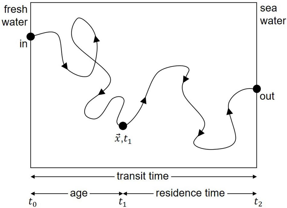
Figure 1. Example illustrating the definitions of time scales according to Zimmerman (1976). The time difference t₁–t₀ from entering the control volume to the actual position x is the “age” of a single water body. The time difference t₂–t₁ from the actual position x to the edge of the control volume is the “residence time” of the water body. The sum of both is the “transit time” covering the time span from entering to leaving the control volume. If many water bodies are considered, the different time scales can be computed for each water body. Averaging over all water bodies results in “mean age”, “mean residence time” or “mean transit time”. Properties such as “turn-over time” (Bolin and Rohde, 1973) or “flushing time” (Zimmerman, 1976) cannot be displayed in this graph because they are defined by total volume divided by total flux. The “influence time” (Delhez et al., 2014) although defined differently, has a similarity to “age”. Consequently, the presence of eddies or loop currents would cause a longer pathway through the control volume and would result in longer time scales. A plot of the residence time as function of the starting point results in the LRT as function of space and time. The area averaged LRT is equivalent to the mean residence time.

According to Zimmerman (1976), the residence time of a water body in a control volume is defined as the time required for the water body to leave that volume (see also Figure 1 and the legend). This concept of residence time has been widely used in different geographic areas (Dippner, 1993; Cucco and Umgiesser, 2006; de Brauwere et al., 2011; Daewel and Schrum, 2013). An alternative approach was that of Delhez et al. (2014), who proposed the concept of influence time, defined as the time required to replace the water in the area of interest by renewing water.

A fundamental problem of these definitions of time scales is that all are based on a fixed reservoir, such that mixing and flushing time scales are geometrically influenced and the dynamics of synoptic or mesoscale variability are not considered. To overcome the problem of geometric fixed volumes, Dippner (1994) developed the concept of dynamic flushing time, which assumes a variable volume that depends on the position of a frontal system. In the present work, we apply a similar approach to compute the local Lagrangian residence time (LRT) for the Bay of Gdańsk (BG) and Vistula River (VR).

Bay of Gdańsk is one of the larger bays in the southern Baltic Sea. The orography is characterized by the Peninsula Hel, which protects the western part of the Bay from the direct influence of the Baltic Sea. Dynamically the BG is a Bay, which is driven by variable wind forcing and the river plume front of VR. The influence of tides is negligible and also the impact of wave induced mass transport is of minor importance as in many other bays (Dippner, 1987).

The VR is one of the largest rivers draining into the southern Baltic Sea, discharging 15% of the total amount of nitrogen and 19% of the total amount of phosphorus from land-based sources into the Baltic Sea (HELCOM, 1998). A determination of the climatologic winter mean (January and February 1928–2005) molar N:P ratio of inorganic nutrients in the upper 30 m of the BG water-column based on monitoring data (Feistel et al., 2008) yielded values close to Redfield ratio (Figure 2). By contrast, N:P values in the surface water of the BG, measured on a cruise of the “FS Elisabeth Mann-Borgese” (29.2.–9.3. 2016), determined very high ratios, up to 7.8 times higher than the Redfield ratio of 16 (Figure 3). Further data obtained during the cruise are reported in Bartl et al. (2018, 2019). The high and unbalanced Redfield ratios in the coastal zone may alter nitrate cycling (Lunau et al., 2012). To understand the efficiency of nitrate removal, nutrient retention capacity and the complexity of the coastal filter function in the BG (Thoms et al., 2018; Bartl et al., 2019) requires knowledge of the water residence time. Based on the LOICZ (Land Ocean Interactions in the Coastal Zone) model of Gordon et al. (1996); Witek et al. (2003) computed a flushing time of 15 days in the BG, which they named “water exchange time” or “water residence time”.

FIGURE 2

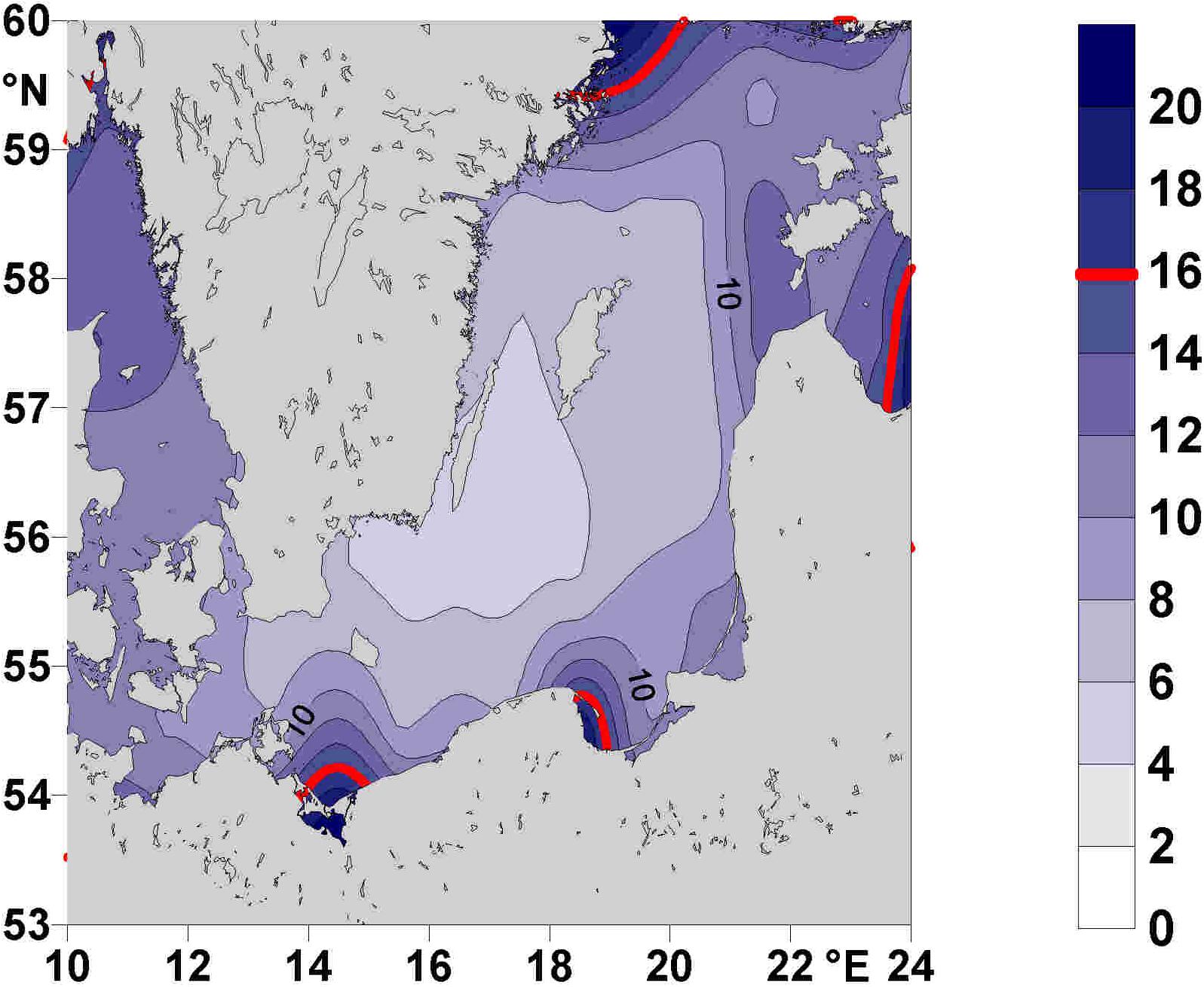
Figure 2. Climatic mean molar N:P ratios during January and February from 1928 to 2005 in the upper 30 m of the Baltic Proper, based on monitoring data compiled by Feistel et al. (2008). The red line indicates the Redfield ratio of 16.

FIGURE 3

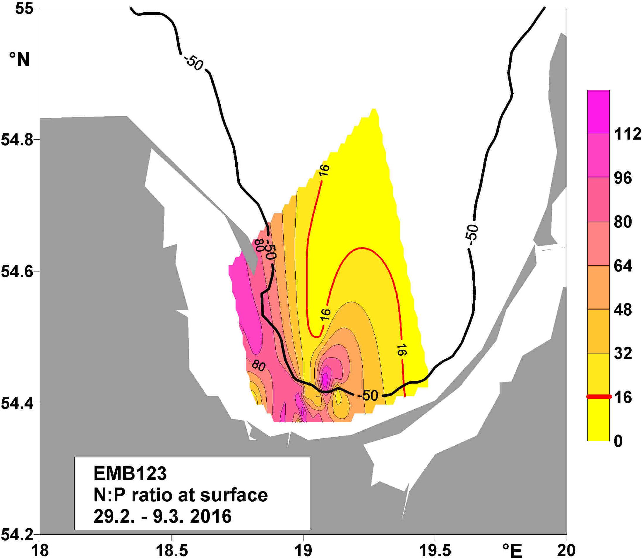
Figure 3. Molar N:P ratio at the surface during cruise EMB123, in spring 2016. The bold line indicates the 50-m depth contour, and the red line the Redfield ratio of 16. The measured maximum was 7.8 times higher than the Redfield ratio.

The disadvantage of the method used by many authors is that a fixed volume and a constant transport rate are assumed. This approach does not consider the dynamics of eddies and river plume fronts. While under normal conditions the VR plume propagates eastward, parallel to the coast, during easterly or northeasterly winds it detaches from the coast and meanders in the center of the BG. The resulting eddies have a seasonal varying radius of deformation of 850 m during winter, 4500 m during spring and 6500 m during summer (Voss et al., 2005; Bartl et al., 2018) and a spin-down time of approximately 4.5 days (Voss et al., 2005). These non-linear processes can be taken into account if the residence time is computed using an eddy-resolving model within a Lagrangian framework. Dippner (1994) showed that the dynamic flushing rates in a Lagrangian coordinate system are much lower than geometric flushing rates. Therefore, we hypothesized that the LRT in the BG is much longer than the estimated 15 days (Witek et al., 2003).

Materials and Methods

The Circulation Model

The circulation model (Holtermann et al., 2014) is an eddy-resolving version of the General Estuarine Transport Model (Burchard and Bolding, 2002). It computes the three-dimensional, non-linear, baroclinic primitive equations in a staggered C-grid (Arakawa and Lamb, 1977), assuming hydrostatic and Boussinesq approximations. The model domain, which covers the Central Baltic Sea with very high resolution, is one-way nested in a coarser resolution model that simulates the entire Baltic Sea. Figure 4 shows the outer (Baltic Sea) and inner (Central Baltic Sea) model domains along with the topography and location of Gdańsk Bay in the model. The adaptive scheme used in the vertical direction follows the evolution of shear and stratification in the interior of the water column (Hofmeister et al., 2010). Advection was discretized using a frontal-conserving total-variation-diminishing scheme, following the directional split approach of Pietrzak (1998). Temporal discretization is based on a mode splitting of barotropic and baroclinic pressure gradients (Backhaus, 1985). Vertical mixing is computed with a second-order k-ε closure scheme that is extended by two prognostic equations for the turbulent kinetic energy k and the dissipation rate ε (Umlauf and Burchard, 2005), and horizontal mixing using the scheme of Smagorinsky (1963). Further details are given in Holtermann et al. (2014).

FIGURE 4

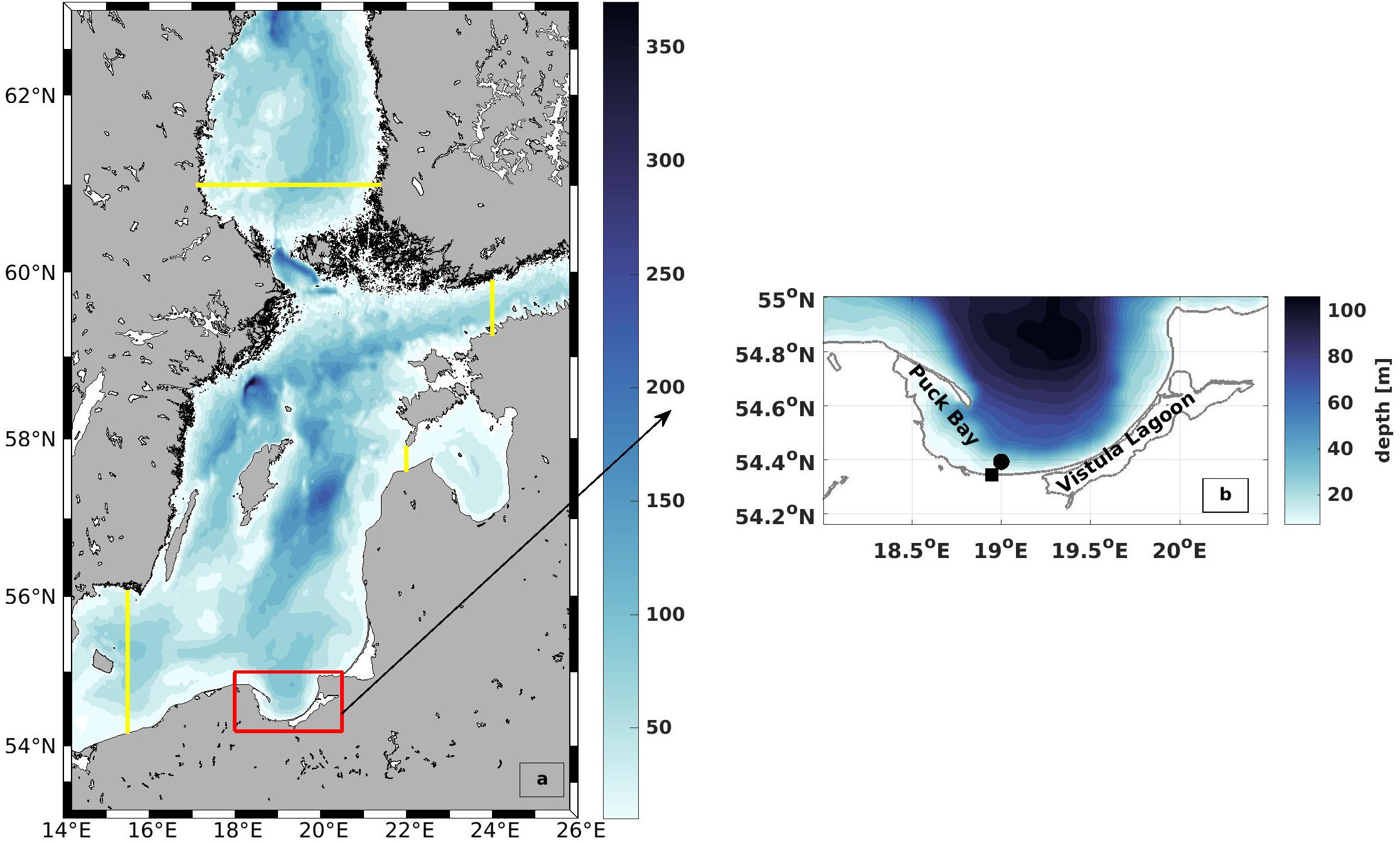
Figure 4. Model domain and bathymetry (a) The outer model along with the inner high resolution model that was used for this research. The yellow lines mark the location of the open boundaries. The red box shows the location of the study area (b) Bathymetry of the Bay of Gdańsk. The black square indicates the entrance of the Vistula River (VR) and the black dot indicates the area of the model wind.

To account for riverine freshwater fluxes, the daily discharges of the Baltic Sea rivers were extracted from the Global Runoff Data Centre database. For the Baltic Sea, only 60% could be covered with direct observations (including the VR). For the remaining rivers, individual climatologic annual cycles were constructed. Afterward, the total annual discharge of all Baltic Sea rivers was computed and compared with the Baltic Marine Environment Protection Commission–Helsinki Commission (HELCOM) estimates (HELCOM, 1986). Then, the climatologically rivers were rescaled such that the sum of observed discharge and scaled climatologically river discharge matched the HELCOM values. The freshwater input of VR, which is the main river in BG, is displayed in Figure 5.

FIGURE 5

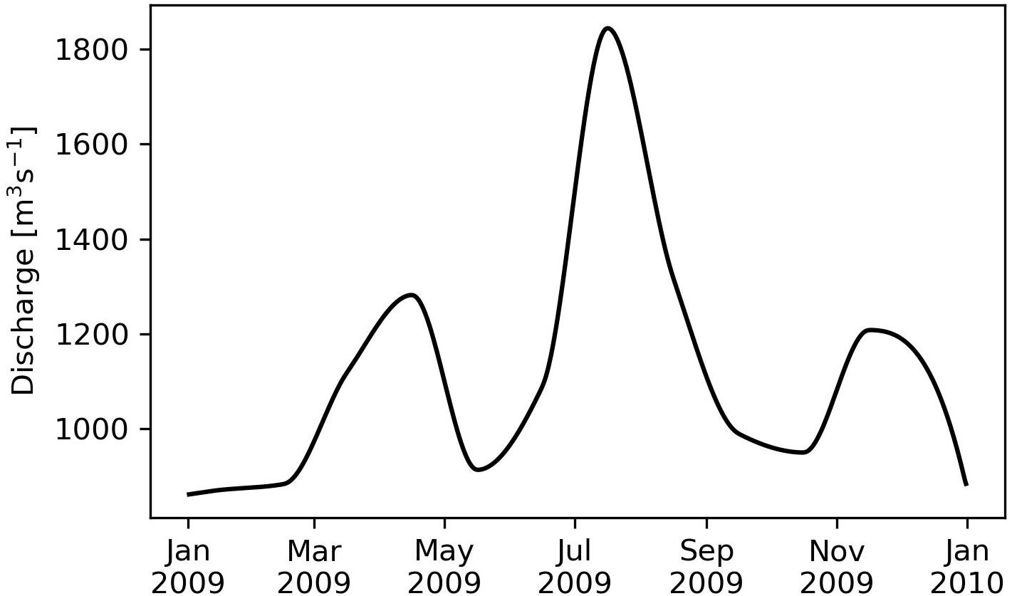
Figure 5. Runoff of VR for 2009 from the Global Runoff Data Center.

The boundary conditions were adopted from a larger-scale model that covers the entire Baltic Sea (Figure 4) with a setup similar to the one used by Hofmeister et al. (2011). The initial conditions were constructed from multiple Conductivity-Temperature-Depth (CTD) profiles and interpolated to the model grid by applying a distance-weighted algorithm. Data on atmospheric fluxes were obtained from the German Weather Service (DWD). Those data are available with 3 h temporal resolution and were used in order to calculate the air–sea fluxes of momentum, heat and humidity based on the bulk formulas of Kondo (1975).

The topography was linearly interpolated from a 1 NM grid (Büchmann et al., 2011). The model has spherical coordinates with a resolution of 0.00914° (501–597 m) and 0.0054° (596 m) for zonal and meridional directions, respectively. The time step is 3 s for the barotropic and 60 s for the baroclinic mode. The results were stored every 3 h. Although the complete model run covers the period 2007–2017 a detailed validation was performed for the years 2007–2009 in order to coincide with the Baltic Sea Tracer Release Experiment (BATRE) (Holtermann et al., 2014).

The model was validated against observed sea level elevations, temperature and salinity profiles at different locations in the Central Baltic Sea and fit well to the observations (Holtermann et al., 2014). For the presented analysis, we use the computed surface velocities of 2009.

The Lagrangian Model

According to Maier-Reimer (1979), the local LRT is computed within a Lagrangian framework. If a water body is interpreted not as a continuum, but as a finite set of water particles transported by the Eulerian velocity field, then each particle is characterized by a co-ordinate x and an age a. Accordingly, the numerical problem of solving an advection–diffusion equation is reduced to the simple problem of solving a set of ordinary differential equations describing the change in coordinates and properties for each particle. Hence, transport, diffusion and age are calculated as described in Eq. 1:

$\begin{array}{c}{\overrightarrow{x}}_i^{t+\mathrm{\Delta }t}={\overrightarrow{x}}_i^t+\mathrm{\Delta }{t}^{*}\left[{\overrightarrow{u}}_L+\left(\mathrm{\mu }-0.5\right)\overrightarrow{P}\right]\hfill \\ a_i^{t+\mathrm{\Delta }t}=a_i^t+\mathrm{\Delta }t\hfill \end{array}(1)$

where i is the i-th particle, t is the time, Δt is the time step, P is a “band-width” of turbulent fluctuation and μ is a random number uniformly distributed between 0 and 1. The advection velocity u_L is obtained from the Eulerian velocity field of the circulation model by transformation onto Lagrangian coordinates (Maier-Reimer, 1988; Dippner, 1990). A reflecting boundary condition for the random walk is used at the closed boundary. From a numerical perspective, the main disadvantage of the Eulerian system is the advective part of the transport equation, which yields the well-known problem of numerical diffusivity, especially in the presence of strong gradients (Dippner, 2005). However, by transformation onto Lagrangian coordinates, which is the core of the technique, this part simply vanishes. For the diffusion part of the equation, which a priori is assumed to be of minor relevance, a simple Monte Carlo technique is used. Eq. 1 is solved using a 4th-order Runge-Kutta method. In this simulation, the particles are advected at the horizontal surface velocities, excluding a vertical component. Thus, the particles can be interpreted as buoyant particles at the surface.

Two different complementary applications were computed to analyze the spatial as well the temporal variability. In the first application, we analyzed the horizontal variability and initialized at each wet grid point of the model a tracer with an age (a = 0d), excluding the Vistula Lagoon and compute the time for all 19,458 tracers required to leave the model domain. This was done with the velocity fields for 2009, beginning January 1st and diffusion (P = 0 m/s) was not considered. This procedure was repeated for all other months starting on the 1st of each month (Figures 6, 7). To estimate the influence of diffusion, the runs were repeated using different diffusion velocities. Figure 8 displays both, the time required for all tracers to leave the model domain (T₁₀₀) and the time at which 95% of the tracers have left the area (T₉₅) for all month and three different diffusion velocities, 0, 0.1, and 0.2 m/s. Averaging over all months yielded an annual mean LRT (Figure 9), with the standard deviation providing information on the spatial variability of the LRT in the BG (Figure 10).

FIGURE 6

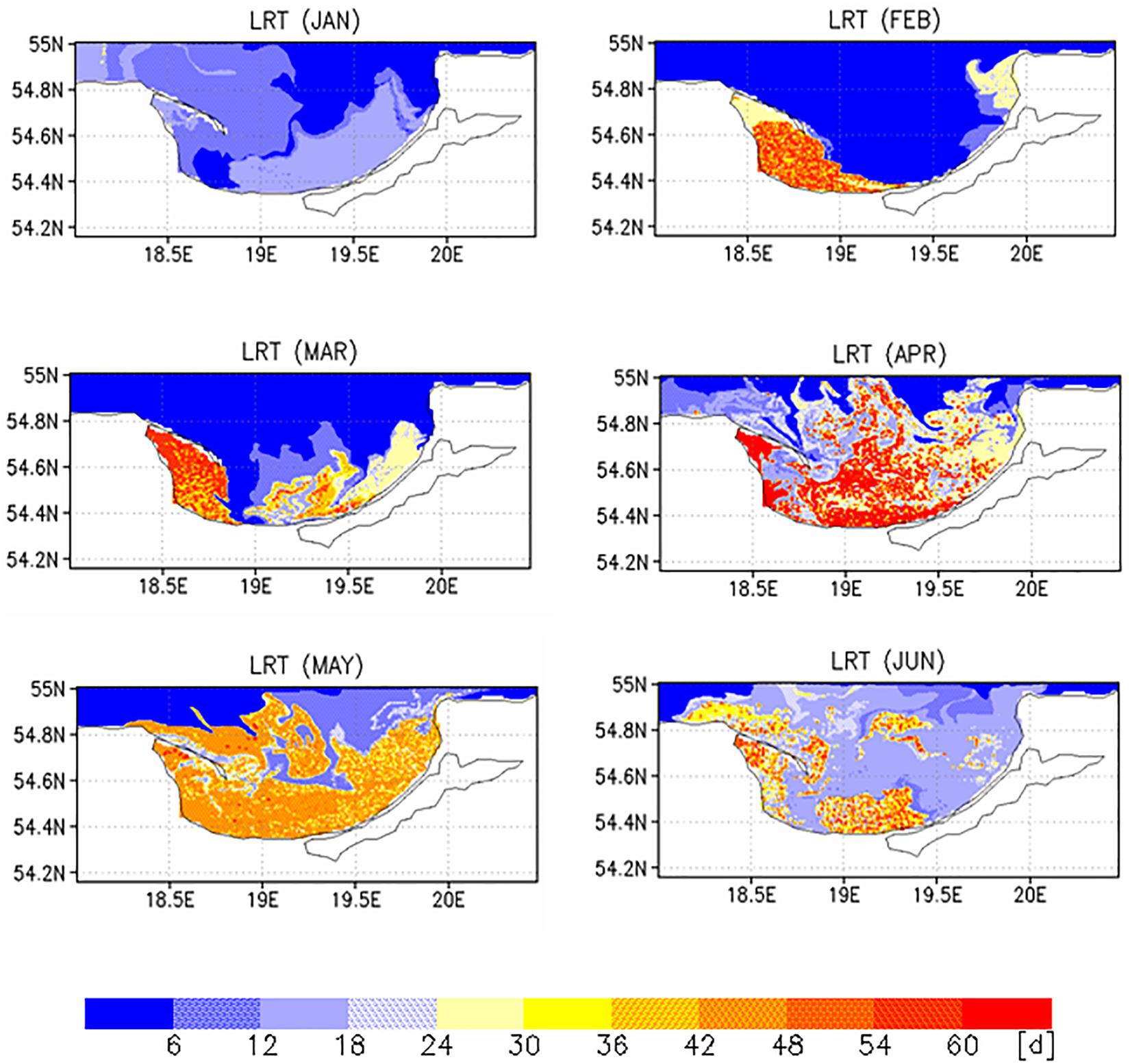
Figure 6. Lagrangian residence time (LRT) in days for January to June 2009.

FIGURE 7

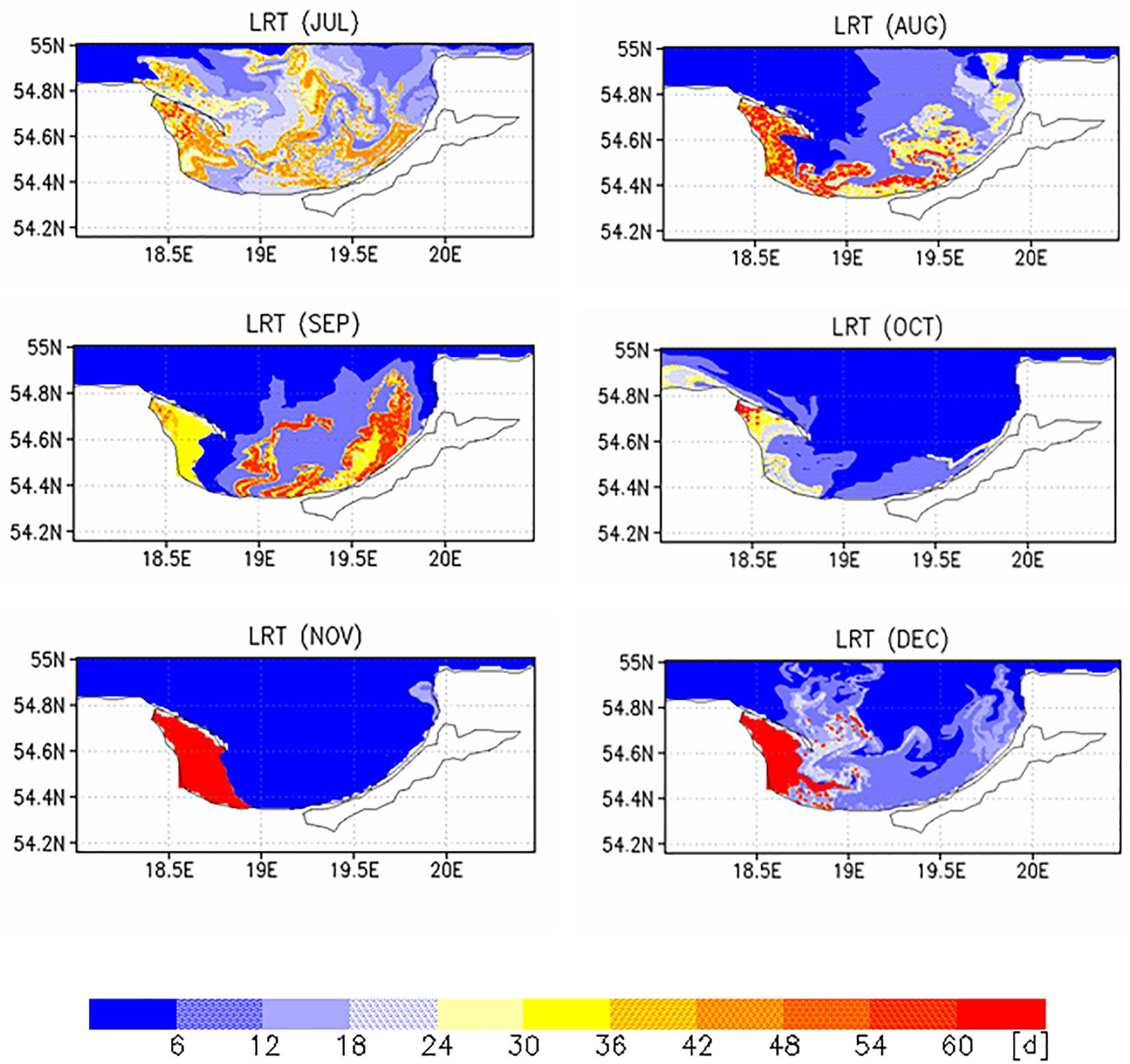
Figure 7. Lagrangian residence time (LRT) in days for July to December 2009.

FIGURE 8

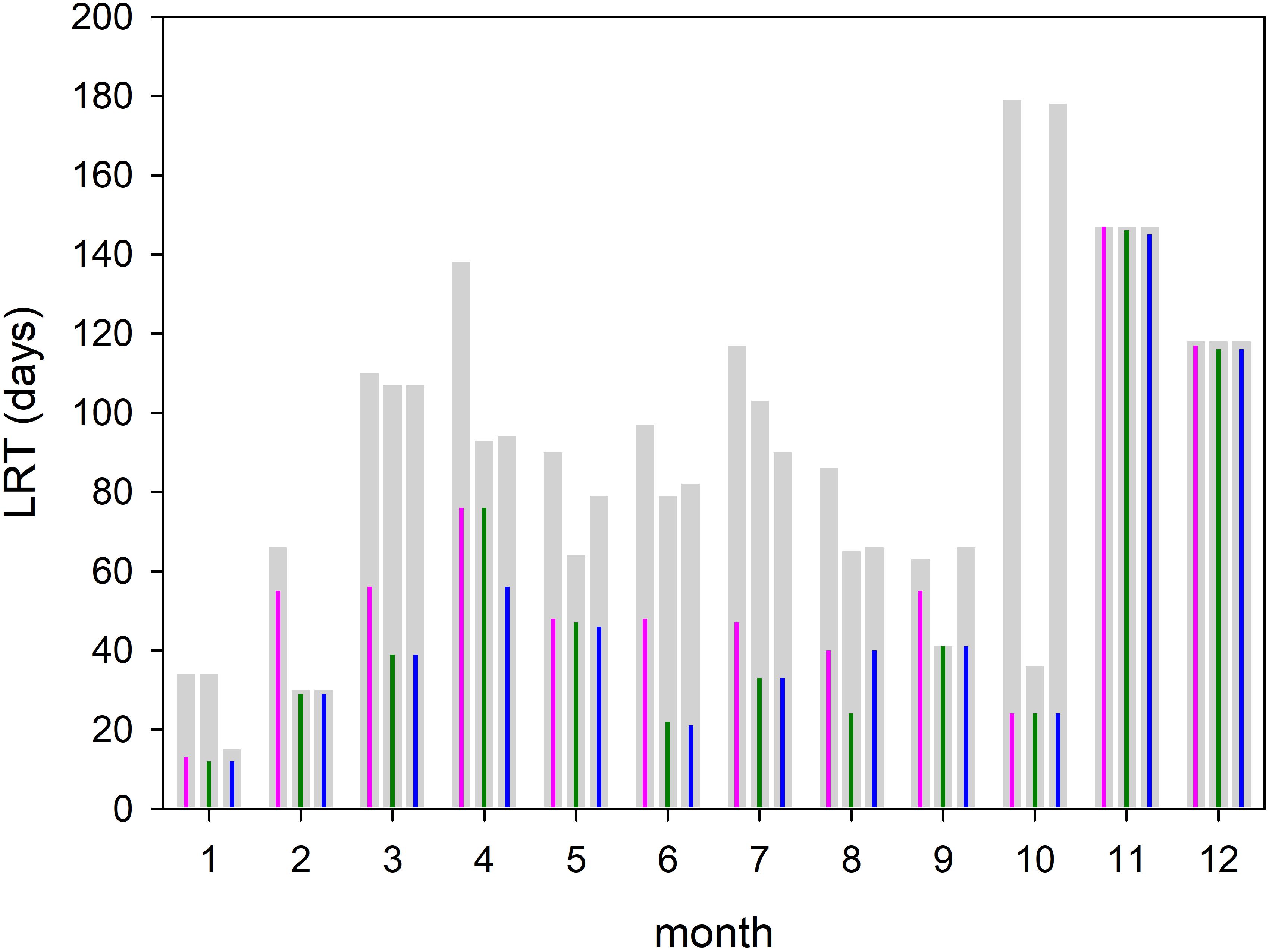
Figure 8. Amount of time required for all tracers (T₁₀₀, gray bars) and 95% of the tracers (T₉₅, colored impulse) to leave the Bay of Gdańsk. The time is computed for each month and different diffusion velocities P = 0 m/s (magenta); P = 0.1 m/s (green), and P = 0.2 m/s (blue).

FIGURE 9

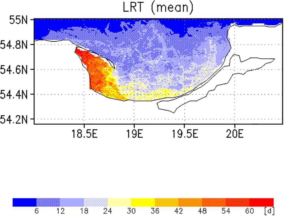
Figure 9. Mean LRT (in days) for the Bay of Gdańsk during 2009.

FIGURE 10

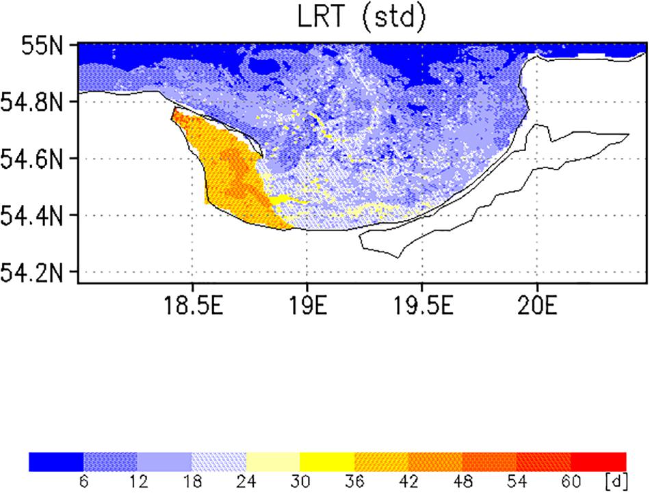
Figure 10. Standard deviation of the LRT (in days) for the Bay of Gdańsk in 2009.

To estimate the LRT of the Vistula plume only and the temporal variability of LRT, in a second application 105,120 tracers were initialized in the vicinity of the VR’s entrance. For 1 year, a tracer was released every 5 min and advected until all tracers had left the domain. The entire computation covered the period from January 1, 2009 to March 28, 2010. With this approach, the LRT is identical to the Lagrangian transit time as shown in Figure 1 (Zimmerman, 1976). The spectra of the LRTs of the tracers and their cumulative spectra were shown in Figure 11. Again to estimate the potential influence of diffusion, the run was repeated using different diffusion velocities. The spectra for diffusion velocities of 0.1 and 0.2 m/s were also shown in Figure 11.

FIGURE 11

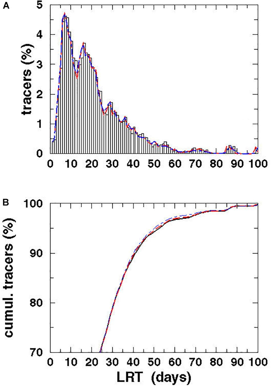
Figure 11. Spectrum (A) and cumulative spectrum (B) of the Lagrangian tracers (%) vs. the LRT for the water of the VR for different diffusion velocities: P = 0 m/s (black), P = 0.1 m/s (red dashed), and P = 0.2 m/s (blue dot-dashed).

Nutrient Export

According to Nixon et al. (1996), the LRT (in months) can be used to compute specific, residence-time-dependent estuarine quantities using the bulk formulas for the export of total nitrogen (TN) and total phosphorus (TP):

$\begin{array}{c}TN=-27\log (LRT)+64.8\hfill \\ TP=-31.83\log (LRT)+80.8\hfill \end{array}(2)$

These bulk formulas were derived from regression analyses of relative TN or TP exports (% of total N or P inputs) as a function of mean water residence time (month) (Nixon et al., 1996, Figures 1, 2 therein). Since the regression analyses are based on data from semi-enclosed estuaries, lagoons and freshwater lakes, their application to the open BG is limited and regarded solely as qualitative estimations of the relative amounts of exported and retained nutrients.

Results

The monthly spatial distributions of the LRT showed rather heterogeneous patterns (Figures 6, 7) and a pronounced intra-annual variability. Details of monthly circulation patterns and wind fields were documented in the Supplementary Information (SI). The shortest LRTs during the considered year were in January and October, which were caused by the dominant southerly to south-westerly winds resulting in a strong flushing. During November, December and February, the longest LRT was in the Puck Bay. These long LRTs were caused by mainly southerly winds from southwest to southeast. The consequence was a stagnant circulation in the Puck Bay affecting long residence times, which can last more than 3 month in November and December (Figures 7, 8). For 95% of the tracers, 147 days beginning in November and 117 days beginning in December were required to leave the bay. The combination of these wind fields with the semi-enclosed geometry of the Puck Bay resulted in the highest mean and standard deviation of the LRT (Figures 9, 10). During these months, the stagnant circulation for longer than 3 months is also influenced by the wind history and the accumulative consequences of the wind forcing (see Supplementary Information).

By contrast, the LRTs during spring and summer were patchy and highly heterogeneous. The annual mean residual circulation in the BG computed from all velocity fields was 1.7 cm/s. Wind fields in opposite direction to the mean circulation resulted in a stronger perturbation of the circulation field, e.g., a detachment of the river plume front from the coast, the formation of baroclinic instabilities and the formation of eddies (Voss et al., 2005). The formation of meandering patterns and filaments clearly reflected the influence of the eddy field and the variability of wind forcing on the LRT (see also Supplementary Information).

Assuming that the T₉₅ value of each month can be considered as a monthly mean residence time (Figure 8), the annual mean residence time, obtained by averaging over all months, was 60 days. If months with extremely low and high values (January and November) were excluded, the averaged residence time was 56 days. Figure 8 also displays the simulations with different diffusion velocities. The colored impulses were the T₉₅ values and the gray bars the T₁₀₀ values for each model run. The T₉₅ values were identical in January, October, November and December, During the other month of the year the differences were small. The T₁₀₀ values showed a lager variability. With respect to most of the T₉₅ values, the time at which 95% of the tracers have left the area, diffusion seems to play a minor role. A possible explanation is given below.

The spatial pattern of the mean LRT (Figure 9), averaged over all months, could be split into three different areas. (i) north of 54.6°N, where the LRT was <24 days; (ii) in Puck Bay, where the LRT was longest, >48 days, and (iii) over a small belt in front of the Polish coast, the near-coastal area, where the LRT was between 24 and 36 days. The water depth in the latter two areas was shallower than 50 m. In the graph of the standard deviation of the LRT (Figure 10), two different areas were identified: in the Puck Bay, where the variability in the LRT was highest, and the western near-coastal area, where the LRT exceeded 36 days. In the rest of the bay the variability in the LRT was <24 days.

Investigating the temporal variability and the fate of VR water, long-term simulations were performed with and without considering diffusion (Figure 8). The spectra as well as the cumulative spectra were identical, indicating that turbulent diffusion might be of minor relevance on this scales. Two larger peaks seen at 7 and 16 days have amplitudes of 4.6% and of 3.7%, respectively, while the minor peak at 29 days had an amplitude of 1.7%. Along with the peaks, the spectra were broad, with a smooth e-folding in its tail and an amplitude of 0.5% until 55 days. A view of the cumulative spectra showed that after 16 days, i.e., close to the estimated flushing time reported by Witek et al. (2003), only 47% of the tracers had left the BG. The LRT of 95% of the tracers was 53 days, which was more than three-fold higher than the value estimated by Witek et al. (2003). No significant changes in the tracer spectra were identified by considering diffusion in the long-term simulation. The maximum speed in the surface velocity was 1.4 m/s, which is large compared to the maximum diffusion velocity of 0.2 m/s. The narrow grid of the eddy-resolving model allows to resolve small scale processes such as stretching and shear deformation, which contribute generally to diffusion. Therefore, an additional diffusion velocity seems to be not necessary in the model.

Based on a LRT of 56 days and using the bulk formulas (Eq. 2) of Nixon et al. (1996), total nutrient export for nitrogen and phosphorus in the surface water of the BG was estimated: 57.5% and 72.2%, respectively. Using the time-averaged (1980–1993) riverine loads of TN (119 kt) and TP (5.5 kt) reported by Stålnacke et al. (1999), the amount of N and P retained on the surface water of the BG was 50.6 and 1.5 kt, respectively.

Discussion

Our results indicate water residence times up to four times longer than the 15 days flushing time estimated by Witek et al. (2003). This difference was remarkable given that we used only the surface velocities. Using the model of Delhez et al. (2014), the computed influence time for surface water in the BG was in the same range as our results (Bartl, pers. comm.), which suggests that the computations of residence time in a Lagrangian model and influence time in a Eulerian model seem to be equivalent. This similarity will be the subject of a future investigation. The potential impact and consequences of the LRT in the surface water of the BG are discussed in the following.

Spatial Differences of LRT

The residence times in Puck Bay were significantly longer than in the rest of the BG, especially in winter (November to March), although it has no allochthonous nutrient source. Puck Bay is characterized by a shallow water depth, effective vertical mixing and a high population density of different benthic communities (Janas et al., 2004). Its sediments provide a large remineralization potential and play a key role in nutrient turnover (Andersen and Kristensen, 1992). Thus, together with the long surface-water LRT, recycled nutrients from the sediments may strongly impact the productivity in Puck Bay.

The 50-m depth contour in the BG (Figure 3) separates near-coastal sandy sediments from offshore muddy sediments (Thoms et al., 2018). This differentiation also appears in the LRT, which was longer in the coastal area shallower than 50 m water depth than in the northern offshore area. The longer surface-water LRT in the near-coastal area may be conducive to the sedimentation of organic matter deriving from primary production on the near-coastal seafloor. This would fuel benthic nutrient turnover, especially nutrient retention via fluxes (Thoms et al., 2018) and nitrification (Bartl et al., 2019), in turn facilitating permanent nutrient-removal processes such as denitrification and burial. Thus, the surface-water LRT may have an indirect impact on the permanent removal of nutrients from this coastal system, which functions on time scales much longer than the mean water residence time (Asmala et al., 2017). By contrast, the bottom water residence time may have a more direct influence than the surface LRT on benthic nutrient retention and permanent nutrient removal. Overall, the water residence time strongly influences how often a nutrient cycles within a coastal system before it is removed or exported. This complex behavior is currently the subject of a detailed model-based study computing the influence time at the surface and bottom of the BG (Bartl, pers. comm.).

Nutrient Cycle and Filter Function

Inputs to the Baltic Sea of TN and TP from rivers, atmospheric deposition and nitrogen fixation have been slowly decreasing since the 1980s and are currently estimated to be 638 kt/year for TN and 28 kt/year for TP. These loads include dissolved inorganic, organic and particulate sources (HELCOM, 2011). Inorganic nutrients in the form of nitrate and phosphate contribute most to the TN (45% dissolved inorganic nitrogen, DIN) and TP (51% dissolved inorganic phosphorus, DIP) loads of the VR (Pastuszak and Witek, 2012).

However, from 1989 to 2006 the DIN concentrations in coastal waters increased (HELCOM, 2009) but since then seem to have stagnated, given the recent decreases in the loads from major rivers (HELCOM, 2011). DIN and DIP loads to the Baltic Proper are roughly 200 kt N and 7 kt P (taken from Figure 3.8, HELCOM, 2009), with a molar N:P ratio of roughly 13, which is in agreement with the long-term climatic mean (Figure 2). Whether this ratio systematically changes in near-coastal areas due to microbial or chemical processes is unknown, but the significantly lower N:P ratio in the Baltic Proper is well documented (Voss et al., 2006). The residence time is the most important factor regulating nutrient cycling (Nixon et al., 1996). Nutrient retention, i.e., the biological cycling of nutrients via their incorporation into biomass and remineralization, slows nutrient transport from the land to the sea whereas nutrient removal via denitrification or burial permanently reduces the inventory (Asmala et al., 2017). Nutrient retention facilitates a nutrient residence time that is longer than the mean water residence time (Asmala et al., 2017), which in turn allows permanent nutrient removal to mitigate riverine nutrient loads in the coastal zone.

In the surface water, the active processes supporting nitrogen retention are the assimilation of inorganic nutrients into biomass and regeneration. Estuarine conditions similar to those of the BG are found in Pomeranian Bay, off the Oder River Lagoon. In a study of that bay by Korth et al. (2013), nitrate assimilation rates of up to 235 nmol N L^–1 h^–1 were determined in March, suggesting daily rates of 2.82 μmol L^–1 d^–1 in the surface waters (1 m water depth, constant rates for 12 daylight h). Assuming similar rates in the near-coastal area of the BG, nitrate assimilation would consume an appreciable amount of 17–152 μmol L^–1 during a LRT of 6–54 days. The nitrate concentration of the VR in March was ∼186 μmol L^–1 (see Figure 9.6 in Pastuszak and Witek, 2012), resulting in a nitrate input of 31–281 μmol L^–1 within 6–54 days, assuming a discharge rate of 1600 m³ s^–1 (see Figure 9.5 in Pastuszak and Witek, 2012) into an estuarine surface water volume of 4.94 km³ (BG surface area × 1 m water depth). Thus ∼54% of riverine nitrate may be incorporated into biomass and thereby retained. A similar quantity (57%) can be estimated using the equation of Nixon et al. (1996), according to which approximately half of the VR’s input is retained and half is exported. The large temporal variability in the LRT and in nitrate uptake rates (Korth et al., 2013) in spring points to a large potential variability in nitrogen retention. Since no nitrate uptake rates are available from other seasons, we can only speculate here. In summer, when primary production is highest (Witek et al., 1999) concurrent with long LRT (Figures 6, 7), all riverine DIN is likely incorporated into biomass. In autumn and winter, however, LRT is short except in the Puck Bay (Figure 7) and primary production (Witek et al., 1999) is low while riverine N loads can be high resulting in pronounced export of N. Consequently, the timing of the surface-water residence time together with nutrient discharges from the VR and nutrient uptake rates determines the efficiency of nutrient retention in the BG.

Half of the plankton biomass resulting from nutrient assimilation was degraded in the surface waters and remineralized to inorganic nutrients within 30 days (Garber, 1984). Since the LRT is similar throughout the spring (March–May) and riverine nutrients are continuously delivered, a bloom could theoretically develop and persist during the spring months. In addition, assimilation and degradation, including ammonification and nitrification, in the coastal surface waters for the entire spring period can be assumed. Indeed, mean nitrification rates of 59 nmol L^–1d^–1 were detected during a spring bloom in the surface waters of the BG, and further offshore they were much higher 258 nmol L^–1d^–1 (Bartl et al., 2018). This observation is consistent with the high N:P ratio in the nutrient load, which is ∼140 in winter and spring but only ∼10 in summer (Voss et al., 2006). The highest Redfield ratios measured in the surface waters of the BG during winter were in Puck Bay and the near-coastal area shallower than 50 m water depth (Figure 3). These ratios are far above the ratio of ∼16:1 needed to meet the metabolic requirements of plankton. An experiment with estuarine water in which a gradient in N:P ratios was applied demonstrated that nitrification rates are significantly enhanced under a surplus of nitrogen (Lunau et al., 2012). A field study along an estuarine gradient also reported a significant increase in nitrification rates at sites where nitrate levels were highest (Dähnke et al., 2008). These two studies independently support enhanced nutrient retention under high N-loads and a sufficient residence time.

Impact of LRT on Genetic Differentiation

The results of this study also help to explain the strong genetic differentiation among phytoplankton populations in the BG. Previous studies of the genetic differentiation of two bloom-forming species in the Baltic Sea, the diatom Skeletonema marinoi and the toxic dinoflagellate Alexandrium ostenfeldii, showed that they were genetically distinct from other local Baltic populations (Tahvanainen et al., 2012; Sjöqvist et al., 2015). Our study showed that the bloom periods for S. marinoi and A. ostenfeldii (February–April and August–September, respectively) were characterized by long residence times, which would prevent transport of the blooms into the main basins and, for LRTs >30 days, facilitate anchoring of the blooming populations in the bay. At the end of their bloom periods, the two species enter a resting stage in which the cells settle to the sea floor, where they form benthic seed banks (Kremp et al., 2009; Godhe and Härnstöm, 2010). Resting stages that accumulate in the inner parts of Puck Bay not only inoculate new local blooms but also facilitate the retention and adaptation of local populations (Sundqvist et al., 2018), which in the case of toxic, bloom-forming A. ostenfeldii will adversely affect both co-occurring biota and public health (Setälä et al., 2014).

Consequences for the Integrated Management of Coastal Zones

Inputs of nitrogen and phosphorus from land into marine coastal systems are responsible for enhanced primary production and therefore eutrophication (Nixon, 1995). According to the Marine Strategy Framework Directive (MSFD, Anonymous, 2008): “Eutrophication is a process driven by enrichment of water by nutrients, especially compounds of nitrogen and/or phosphorus, leading to: increased growth, primary production and biomass of algae; changes in balance of organisms, and water quality degradation. The consequences of eutrophication are undesirable if they appreciably degrade ecosystem health and/or the sustainable provision of goods and services” (Ferreira et al., 2010). The consequences of large-scale eutrophication in the Baltic Sea include reduced water transparency, oxygen depletion, and changes in the marine food web (Fonselius, 1972; Bonsdorff et al., 1997; Karlson et al., 2002; Conley et al., 2011; Voss et al., 2011; Gustafsson et al., 2012).

In addition to being the most important factor regulating nutrient cycling, residence time determines the nutrient retention time, total nutrient export (nitrogen and phosphorus), and the total removal (buried and denitrification) of nitrogen (Nixon et al., 1996). In addition, the LRT is of major relevance for the persistence of harmful contaminants or pollutants as well as toxic algal blooms and influences the efficiency of coastal filter function. All these aspects must be considered in assessments of good environmental status using the MSFD descriptors “biological diversity,” “food web,” “eutrophication” and “seafloor integrity.” However, the Task Group Reports on “Biological diversity” (Cochrane et al., 2010), “Food webs” (Rogers et al., 2010), “Eutrophication” (Ferreira et al., 2010) and “Seafloor integrity” (Rice et al., 2010) do not explicitly consider residence time as an important variable influencing and regulating processes in near-coastal marine ecosystems. MSFD descriptor 5 (eutrophication) refers to the adverse effects of eutrophication as including “losses in biodiversity, ecosystem degradation, harmful algae blooms and oxygen deficiency in bottom waters” (Ferreira et al., 2010). Nonetheless, because eutrophication is strongly linked with the other MSFD descriptors mentioned above, via strong bentho-pelagic coupling, residence time is an important driver for all of them. The incorporation of residence time into these MSFD descriptors would result in an improved, unbiased evaluation of good environmental status.

These considerations are also of major relevance in the context of nutrient reduction efforts. Conley (2000) suggested that a reduction in phosphorus loads in spring will contribute to reducing both oxygen deficiency and fast-growing macrophytes, whereas a reduction in nitrogen loads would reduce summer chlorophyll concentrations and improve the conditions for benthic vegetation. A much larger residence time during summer would result in a prolongation of high-levels algal biomass production. To avoid undesirable algal blooms, reductions of both nitrogen and phosphorus are urgently required for the conservation of near-coastal areas and for the achievement of a good ecological status.

Data Availability Statement

The model results supporting the conclusion of this manuscript will be made available by the authors, without undue reservation, to any qualified researcher.

Author Contributions

JD, EC, and PH made the computations. IB, AK, FT, and MV contributed to the text.

Funding

EC was the recipient of support for the project T2 (Energy Budget of the Ocean Surface Mixed Layer) of the Collaborative Research Centre TRR 181 on Energy Transfer in Atmosphere and Ocean, funded by the German Research Foundation–project number 274762653. IB and FT were funded through the BONUS COCOA project, by BMBF grant number FKZ 03F063A. PH was financed by grant HO5891/1-1, from the German Research Foundation. Additional support was received by the Open Access Fund of the Leibniz Association.

Conflict of Interest

The authors declare that the research was conducted in the absence of any commercial or financial relationships that could be construed as a potential conflict of interest.

Acknowledgments

The runoff data from Vistula River has been provided by the Global Runoff Data Centre, Koblenz, which is greatly acknowledged.

Supplementary Material

The Supplementary Material for this article can be found online at: https://www.frontiersin.org/articles/10.3389/fmars.2019.00725/full#supplementary-material

References

Andersen, F. Ø., and Kristensen, E. (1992). The importance of benthic macrofauna in decomposition of microalgae in a coastal marine sediment. Limnol. Oceanogr. 37, 1392–1403. doi: 10.4319/lo.1992.37.7.1392

CrossRef Full Text | Google Scholar

Anonymous, (2008). Marine strategy framework directive: directive 2008/56/EC of the European Parliament and of the Council of 17 June 2008 establishing a framework for community action in the field of marine environmental policy (Marine strategy framework directive). Official J. Eur. Union 164, 19–40.

Google Scholar

Arakawa, A., and Lamb, V. (1977). Computational design of the basic dynamical processes of the UCLA general circulation model. Methods Comput. Phys. 17, 173–265. doi: 10.1016/b978-0-12-460817-7.50009-4

CrossRef Full Text | Google Scholar

Asmala, E., Carstensen, J., Conley, D. J., Slomp, C. P., Stadmark, J., and Voss, M. (2017). Efficiency of the coastal filter: nitrogen and phosphorus removal in the Baltic Sea. Limnol. Oceanogr. 62, S222–S238. doi: 10.1007/s13280-019-01282-y

PubMed Abstract | CrossRef Full Text | Google Scholar

Backhaus, J. O. (1985). A three-dimensional model for the simulation of shelf sea dynamics. Dt. Hydrogr. Z. 38, 165–187. doi: 10.1121/1.3605565

PubMed Abstract | CrossRef Full Text | Google Scholar

Bartl, I., Hellemann, D., Rabouille, C., Schulz, K., Tallberg, P., Hietanen, S., et al. (2019). Particulate organic matter controls benthic microbial N retention and N removal in contrasting estuaries of the Baltic Sea. Biogeosciences 16, 3543–3564. doi: 10.5194/bg-16-3543-2019

CrossRef Full Text | Google Scholar

Bartl, I., Liskow, I., Schulz, K., Umlauf, L., and Voss, M. (2018). River plume and bottom boundary layer – Hotspots for nitrification in a coastal bay? Estuar. Coast. Shelf Sci. 208, 70–82. doi: 10.1016/j.ecss.2018.04.023

CrossRef Full Text | Google Scholar

Bolin, B., and Rohde, H. (1973). A note on concepts of age distribution and transit time in natural reservoirs. Tellus 25, 58–62. doi: 10.3402/tellusa.v25i1.9644

CrossRef Full Text | Google Scholar

Bonsdorff, E., Blomquist, E., Mattila, J., and Norkko, A. (1997). Coastal eutrophication: causes, consequences and perspectives in the archipelago areas of the northern Baltic Sea. Estuar. Coast. Shelf Sci. 44, 63–72. doi: 10.1016/s0272-7714(97)80008-x

CrossRef Full Text | Google Scholar

Büchmann, B., Hansen, C., and Söderquist, J. (2011). Improvement of hydrodynamics forecasting of Danish waters: impact of low-frequency North Atlantic barotropic variations. Ocean Dyn. 61, 1611–1617. doi: 10.1007/s10236-011-0451-2

CrossRef Full Text | Google Scholar

Burchard, H., and Bolding, K. (2002). GETM – A General Estuarine Transport Model. Scientific Documentation Tech. Rep. EUR 20253. Ispra: European Commission.

Google Scholar

Cochrane, S. K. J., Conner, D. W., Nilsson, P., Mitchell, I., Reker, J., Franco, J., et al. (2010). Marine Strategy Framework Directive. Guidance on the Interpretation and Application of Descriptor 1: Biological Diversity. Report by Task Group 1 on Biological Diversity for the European Commission’s Joint Research Centre. Luxembourg: Publications Office of the European Union.

Google Scholar

Conley, D. J. (2000). Biogeochemical nutrient cycles and nutrient management strategies. Hydrobiologia 410, 87–96. doi: 10.1007/978-94-017-2163-9_10

CrossRef Full Text | Google Scholar

Conley, D. J., Carstensen, J., Aigars, J., Axell, P., Bonsdorff, E., Eremenia, T., et al. (2011). Hypoxia is increasing in the coastal zone of the Baltic Sea. Environ. Sci. Technol. 45, 6777–6783. doi: 10.1021/es201212r

PubMed Abstract | CrossRef Full Text | Google Scholar

Cucco, A., and Umgiesser, G. (2006). Modeling the Venice lagoon residence time. Ecol. Model. 193, 34–51. doi: 10.1016/j.ecolmodel.2005.07.043

CrossRef Full Text | Google Scholar

Daewel, U., and Schrum, C. (2013). Simulating long-term dynamics of the coupled North Sea and Baltic Sea ecosystem with ECOSMO II: model description and validation. J. Mar. Syst. 119-120, 30–49. doi: 10.1016/j.jmarsys.2013.03.008

CrossRef Full Text | Google Scholar

Dähnke, K., Bahlmann, E., and Emeis, K. (2008). A nitrate sink in estuaries? An assessment of means by stable nitrate isotopes in the Elbe estuary. Limnol. Oceanogr. 53, 1504–1511. doi: 10.4319/lo.2008.53.4.1504

CrossRef Full Text | Google Scholar

de Brauwere, A., de Brye, B., Blaise, S., and Deleersnider, E. (2011). Residence time, exposure time and connectivity in the Scheldt Estuary. J. Mar. Syst. 84, 85–95. doi: 10.1016/j.jmarsys.2010.10.001

CrossRef Full Text | Google Scholar

Delhez, E. J. M., de Brye, B., de Brauwere, A., and Deleersnider, E. (2014). Residence time vs influence time. J. Mar. Syst. 132, 185–195. doi: 10.1016/j.jmarsys.2013.12.005

CrossRef Full Text | Google Scholar

Dippner, J. W. (1987). A swell model of the German Bight. Coast. Eng. 11, 527–538. doi: 10.1016/0378-3839(87)90025-1

CrossRef Full Text | Google Scholar

Dippner, J. W. (1990). Eddy-resolving modelling with dynamically active tracers. Cont. Shelf Res. 10, 87–101. doi: 10.1016/0278-4343(90)90037-m

CrossRef Full Text | Google Scholar

Dippner, J. W. (1993). A Lagrangian model of phytoplankton growth dynamics for the Northern Adriatic Sea. Cont. Shelf Res. 13, 331–355.

Google Scholar

Dippner, J. W. (1994). Dynamic versus geometric flushing rates. Cont. Shelf Res. 14, 313–319. doi: 10.1016/0278-4343(94)90019-1

CrossRef Full Text | Google Scholar

Dippner, J.W. (2005). “Mathematical modelling of the transport of pollution in the water,” in Mathematical Models, ed. J.A. Filar (EOLSS Publishers: Oxford).

Google Scholar

Feistel, R., Nausch, G., and Wasmund, N. (eds) (2008). State and Evolution of the Baltic Sea 1952-2005 – A Detailed 50 Year Survey of Meteorology and Climate, Physics, Chemistry Biology, and Marine Environment (Hoboken NJ: John Wiley & Sons Inc).

Google Scholar

Ferreira, J. G., Andersen, J. H., Borja, A., Bricker, S. B., Camp, J., Cardoso da Silva, M., et al. (2010). Marine Strategy Framework Directive Task Group 5 Report: Eutrophication. Belgium: JRC Scientific and Technical Reports.

Google Scholar

Fonselius, S.H. (1972). “On eutrophication and pollution in the Baltic Sea,” in Marine Pollution and Sea Life, ed. M. Ruivo (London: Fishing News), 23–28.

Google Scholar

Garber, J. H. (1984). Laboratory study of nitrogen and phosphorus remineralization during decomposition of coastal plankton and seston. Estuar. Coast. Shelf Sci. 18, 685–702. doi: 10.1016/0272-7714(84)90039-8

CrossRef Full Text | Google Scholar

Godhe, A., and Härnstöm, A.-S. (2010). Linking the planktonic and benthic habitat: genetic structure of the marine diatom Skeletonema marinoi. Mol. Ecol. 19, 4478–4490. doi: 10.1111/j.1365-294X.2010.04841.x

PubMed Abstract | CrossRef Full Text | Google Scholar

Gordon, D. C., Boudreau, R. P., Mann, K. H., Ing, J.-E., Silvert, W. L., Smith, S. V., et al. (1996). LOICZ biogeochemical modeling guidelines. LOICZ Rep. Stud. 5, 1–96.

Google Scholar

Gustafsson, B. G., Schenk, F., Blenckner, T., Eilola, K., Meier, H. E. M., Müller-Karulis, B., et al. (2012). Reconstructing the development of Baltic Sea eutrophication 1850-2006. Ambio 41, 534–548. doi: 10.1007/s13280-012-0318-x

PubMed Abstract | CrossRef Full Text | Google Scholar

Hainbucher, D., Backhaus, J. O., and Pohlmann, T. (1986). Atlas of Climatological and Actual Seasonal Circulation Patterns in the North Sea and Adjacent Regions, 1969-1981. Hamburg: Institut für Meereskunde.

Google Scholar

HELCOM, (1986). Water balance of the Baltic Sea. Baltic Sea Environ. Proc. 16:174

Google Scholar

HELCOM, (1998). The third pollution load compilation. Baltic Sea Environ. Proc. 32:58

Google Scholar

HELCOM, (2009). Eutrophication in the Baltic Sea - An integrated thematic assessment of the effects of nutrient enrichment, Helsinki Commission. Baltic Sea Environ. Proc. 115B:152

Google Scholar

HELCOM, (2011). Fifth pollution load compilation - PLC5. Baltic Sea Environ. Proc. 2011:217

Google Scholar

Hofmeister, R., Beckers, J.-M., and Burchard, H. (2011). Realistic modelling of the exceptional inflows into the central Baltic Sea in 2003 using terrain-following coordinates. Ocean Model. 39, 233–247. doi: 10.1016/j.ocemod.2011.04.007

CrossRef Full Text | Google Scholar

Hofmeister, R., Burchard, H., and Beckers, J.-M. (2010). Non-uniform adaptive vertical grids for 3D numerical ocean models. Ocean Model. 33, 70–86. doi: 10.1016/j.ocemod2009.12.003

CrossRef Full Text | Google Scholar

Holtermann, P. L., Burchard, H., Gräwe, U., Klingbeil, K., and Umlauf, L. (2014). Deep-water dynamics and boundary mixing in a non-tidal stratified basin: a modeling study of the Baltic Sea. J. Geophys. Res. Oceans 119, 1465–1487. doi: 10.1002/2013JC009483

CrossRef Full Text | Google Scholar

Janas, U., Wocial, J., and Szaniawska, A. (2004). Seasonal and annual changes in the macrozoobenthic populations of the Gulf of Gdańsk with respect to hypoxia and hydrogen sulphide. Oceanologia 46, 85–102.

Google Scholar

Jouon, A., Douillet, P., Ouillon, S., and Fraunié, P. (2006). Calculation of hydrodynamic time parameters in a semi-opened coastal zone using a 3D hydrodynamic model. Cont. Shelf Res. 26, 395–1415.

Google Scholar

Karlson, K., Rosenberg, R., and Bonsdorff, E. (2002). Temporal and spatial large-scale effects of eutrophication and oxygen deficiency on benthic fauna in Scandinavian and Baltic waters: a review. Oceanogr. Mar. Biol. Ann. Rev. 40, 427–489. doi: 10.1201/9780203180594.ch8

CrossRef Full Text | Google Scholar

Kondo, J. (1975). Air–sea bulk transfer coefficients in diabatic conditions. Boundary Layer Meteorol. 9, 91–112 doi: 10.1007/bf00232256

CrossRef Full Text | Google Scholar

Korth, F., Fry, B., Liskow, I., and Voss, M. (2013). Nitrogen turnover during the spring outflows of the nitrate-rich Curonian and Szczecin lagoons using dual nitrate isotopes. Mar. Chem. 154, 1–11. doi: 10.1016/j.marchem.2013.04.012

CrossRef Full Text | Google Scholar

Kremp, A., Lindholm, T., Dreßler, N., Erler, K., Gerdts, G., Eirtovaara, S., et al. (2009). Bloom forming Alexandrium ostenfeldii (Dinophyceae) in shallow waters of the Åland archipelago, Northern Baltic Sea. Harmful Algae 8, 318–328. doi: 10.1016/j.hal.2008.07.004

CrossRef Full Text | Google Scholar

Lunau, M., Voss, M., Erickson, M., Dziallas, C., Casciotti, K., and Ducklow, H. (2012). Excess nitrate loads to coastal waters reduces nitrate removal efficiency: mechanism and implications for coastal eutrophication. Environ. Microbiol. 15, 1492–1504. doi: 10.1111/j.1462-2920.02773.x

PubMed Abstract | CrossRef Full Text | Google Scholar

Maier-Reimer, E. (1979). Some effects of the Atlantic circulation and of river discharges on the residual circulation of the North Sea. Dt. Hydrogr. Z. 32, 126–130. doi: 10.1007/bf02227000

CrossRef Full Text | Google Scholar

Maier-Reimer, E. (1988). Vorticity balance in gulfstream trajectories. Ocean Model. 76, 9–11.

Google Scholar

Nixon, S. W. (1995). Coastal marine eutrophication: a definition, social causes, and future concerns. Ophelia 41, 199–219. doi: 10.1080/00785236.1995.10422044

CrossRef Full Text | Google Scholar

Nixon, S. W., Ammerman, J. W., Atkinson, L. P., Berounsky, V. M., Billen, G., Boicourt, W. C., et al. (1996). The fate of nitrogen and phosphorus at the land-sea margin of the North Atlantic Ocean. Biogeochemistry 35, 141–180. doi: 10.1007/978-94-009-1776-7_4

CrossRef Full Text | Google Scholar

Otto, L. (1978). The transit time distribution for the waters along the Netherlands coast. Oceanol. Acta 1, 31–38.

Google Scholar

Pastuszak, M., Witek, Z. (2012). “Discharges of water and nutrients by the vistula and oder rivers draining polish territory,” in Temporal and Spatial Differences in Emission of Nitrogen and Phosphorus from Polish Territory to the Baltic Sea, eds M. Pastuszak., J. Igras, (Gdynia: National Marine Fisheries Research Institute), 309–346.

Google Scholar

Pietrzak, J. D. (1998). The use of TVD limiters for forward-in-time upstream-biased advection schemes in ocean modelling. Mon. Weather Rev. 126, 812–830. doi: 10.1175/1520-0493(1998)126<0812:tuotlf>2.0.co;2

CrossRef Full Text | Google Scholar

Rice, J., Arvanitidis, C., Borja, A., Frid, C., Hiddink, J., Krause, J., et al. (2010). Marine Strategy Framework Directive Task Group 6 Report: Seafloor Integrity. Belgium: JRC Scientific and Technical Reports.

Google Scholar

Rogers, S., Casini, M., Cury, P., Heath, M., Irigoien, X., Kuosa, H., et al. (2010). Marine Strategy Framework Directive Task Group 4 Report: Food Webs. Belgium: JRC Scientific and Technical Reports.

Google Scholar

Setälä, O., Lehtinen, S., Kremp, A., Hakanen, P., Kankaanpää, H., Erler, K., et al. (2014). Bioaccumulation of PSTs produced by Alexandrium ostenfeldii in the northern Baltic Sea. Hydrobiologia 726, 143–154. doi: 10.1007/s10750-013-1762-8

CrossRef Full Text | Google Scholar

Sjöqvist, C., Godhe, A., Jonsson, P. R., Sundqvist, L., and Kremp, A. (2015). Local adaptation and oceanographic connectivity patterns explain genetic differentiation of a marine diatom across the North Sea–Baltic Sea salinity gradient. Mol. Ecol. 24, 2871–2885. doi: 10.1111/mec.13208

PubMed Abstract | CrossRef Full Text | Google Scholar

Smagorinsky, J. (1963). General circulation experiments with the primitive equations. Mon. Weather Rev. 91, 99–164. doi: 10.1115/1.4027610

PubMed Abstract | CrossRef Full Text | Google Scholar

Stålnacke, P., Grimvall, A., Sundblad, K., and Tonderski, A. (1999). Estimation of riverine loads of nitrogen and phosphorus to the Baltic Sea, 1970-1993. Environ. Monit. Assess. 58, 173–200.

Google Scholar

Sundqvist, L., Godhe, A., Jonsson, P. R., and Sefbom, J. (2018). The anchoring effect—long-term dormancy and genetic population structure. ISME J. 12, 2929–2941. doi: 10.1038/s41396-018-0216-8

PubMed Abstract | CrossRef Full Text | Google Scholar

Tahvanainen, P., Alpermann, T. J., Figueroa, R. I., John, U., Hakanen, P., Nagai, S., et al. (2012). Patterns of post-glacial genetic differentiation in marginal populations of a marine microalga. PLoS One 7:e53602. doi: 10.1371/journal.pone.0053602

PubMed Abstract | CrossRef Full Text | Google Scholar

Thoms, F., Burmeister, C., Dippner, J. W., Gogina, M., Janas, U., Kendzierska, H., et al. (2018). Impact of macrofaunal communities on the coastal filter function in the Bay of Gdańsk, Baltic Sea. Front. Mar. Sci. 5:201. doi: 10.3389/fmars.2018.00201

CrossRef Full Text | Google Scholar

Umlauf, L., and Burchard, H. (2005). Second-order turbulence closure models for geophysical boundary layers. A review of recent work. Cont. Shelf Res. 25, 795–827 doi: 10.1016/j.csr.2004.08.004

CrossRef Full Text | Google Scholar

Voss, M., Deutsch, B., Elmgren, R., Humborg, C., Kuuppo, P., Pastuszak, M., et al. (2006). Source identification of nitrate by means of isotopic tracers in the Baltic Sea catchments. Biogeosciences 3, 663–676. doi: 10.5194/bg-3-663-2006

CrossRef Full Text | Google Scholar

Voss, M., Dippner, J. W., Humborg, C., Hürdler, J., Korth, F., Neumann, T., et al. (2011). History and scenarios of future development of Baltic Sea eutrophication. Estuar. Coast. Shelf Sci. 92, 307–322. doi: 10.1016/j.ecss.2010.12.037

CrossRef Full Text | Google Scholar

Voss, M., Liskow, I., Pastuszak, M., Rüß, D., Schulte, U., and Dippner, J. W. (2005). Riverine discharge into a coastal bay: a stable isotope study in the Gulf of Gdańsk, Baltic Sea. J. Mar. Syst. 57, 127–145. doi: 10.1016/j.jmarsys.2005.04.002

CrossRef Full Text | Google Scholar

Witek, Z., Humborg, C., Savchuk, O., Grelowski, A., and Lysiak-Pastuszak, E. (2003). Nitrogen and phosphorus budgets of the Gulf of Gdańsk (Baltic Sea). Estuar. Coast. Shelf Sci. 57, 239–248. doi: 10.1016/s0272-7714(02)00348-7

CrossRef Full Text | Google Scholar

Witek, Z., Ochocki, S., Nakonieczny, J., Podgórska, B., and Drgas, A. (1999). Primary production and decomposition of organic matter in the epipelagic zone of the Gulf of Gdańsk, an estuary of the Vistula. ICES J. Mar. Sci. 56, 3–14. doi: 10.1006/jmsc.1999.0619

CrossRef Full Text | Google Scholar

Zimmerman, J. T. F. (1976). Mixing and flushing of tidal embayments in the western Dutch Wadden Sea part I: distribution of salinity and calculation of mixing time scales, Netherlands. J. Sea Res. 10, 149–191. doi: 10.1016/0077-7579(76)90013-2

CrossRef Full Text | Google Scholar