Applications of the Gulf of Maine Operational Forecast System to Enhance Spatio-Temporal Oceanographic Awareness for Ocean Mapping

Introduction

Recent technological advances in seafloor mapping systems have greatly improved the quality and the efficiency of data acquisition (Mayer, 2014; Hughes Clarke, 2018; Lamarche and Lurton, 2018). Nevertheless, the resulting products (e.g., bathymetric grids, acoustic backscatter mosaics) and the overall operational efficiency of surveys are often affected by the poor awareness of the oceanographic environment in which the surveys are conducted (Lurton et al., 2015; Hughes Clarke et al., 2017; Mayer et al., 2018).

If the timing of sound speed casts does not properly capture the spatio-temporal variability of the ocean environment, the under-sampled water column produces refraction-induced depth biases in the collected soundings (Beaudoin, 2010; Wilson et al., 2013; Lucieer et al., 2016). Such refraction-induced depth biases can quickly cause the survey to exceed the allowable error tolerances prescribed by best practices and by international and national survey specifications (UKHO, 2004; IHO, 2011; NOAA, 2019a). Along with the sound speed profile, which is critical for ray-tracing, knowledge of the temperature and the salinity variability is crucial in the calculation of appropriate absorption coefficients for acoustic backscatter processing (Masetti et al., 2017; Malik et al., 2018; Montereale-Gavazzi et al., 2019). To summarize, a poor understanding of the oceanographic environment will inevitably lead to increased processing time and effort and may even lead to the need to acquire additional data (Hughes Clarke, 2012; Lecours et al., 2015; Weber et al., 2018). The cautious surveyor will often adopt an approach that overestimates the effects of oceanographic variability by either reducing the sonar swath aperture (and thus affecting the survey efficiency due to the reduced swath coverage) or over-sampling the water column using underway profilers, with the associated wear and tear related costs (Masetti et al., 2018).

Given the current level of predictability of the oceanographic environment, the situation described above can be easily addressed. Increasingly reliable nowcast and forecast guidance from operational oceanographic forecast modeling systems – from local to global scales – are publicly available for key environmental variables (e.g., water temperature and salinity), but they are often not used by ocean mappers (Dudhia, 2014; Bauer et al., 2015; Tonani et al., 2015; Powers et al., 2017; Masetti et al., 2018). This is likely due to the limited awareness of these predictions and the lack of tools that easily allow surveyors to transform model predictions into the estimated effects on the survey data as well as the limited number of studies that have shown the potential benefits incorporating modeled data (Beaudoin et al., 2013; Ros, 2018; Sowers et al., 2019). With the intent of bridging this gap, this study evaluates possible ocean mapping applications for publicly available oceanographic predictions by focusing on one of the available regional models: NOAA National Ocean Service’s Gulf of Maine Operational Forecast System (GoMOFS) (Yang et al., 2016). The GoMOFS was selected because the Gulf of Maine, a semi-enclosed coastal basin along the United States east coast, has a wide variety of physical oceanographic phenomena (from a complex circulation system to strong tidal currents) varying both spatially and seasonally (more details on the model are provided in section “The NOAA’s Gulf of Maine Operational Forecast System”). Thus, a good part of the study’s outcomes should be applicable to other forecast modeling systems of similar (or less) complexity.

The traditional approach to characterizing the water column for ocean mapping aims has been to deploy instruments from a stationary vessel (i.e., performing a hydrocast). Such an approach requires the cessation of mapping for the duration of the cast, directly impacting survey efficiency. With this traditional approach, the ocean mapper is called upon to maintain a balance between the loss in survey efficiency from each new cast and the benefits in terms of improved water column characterization (Beaudoin, 2010; Lucieer et al., 2016; Ros, 2018). The advent of expendable probes has not substantially changed this challenge since the reduced loss of profiling time is offset by the decreased accuracy of the probes relative to a traditional hydrocast, the cost of each expendable probe (combined with the environmental impact of abandoning the used probe on the ocean seafloor). Modern ocean mapping surveys are increasingly adopting underway profilers that can sample the water column at very high rates with the vessel in motion (Furlong et al., 2006; Rudnick and Klinke, 2007). Although those profilers may considerably improve the survey efficiency, the identification of the proper balance between the desired spatio-temporal knowledge of the water column and the working load of the profilers (with associated higher risk of losing the towed probe) is also required (Hughes Clarke et al., 2000; Beaudoin, 2010).

By leveraging predictions from GoMOFS, this study explores two main use cases: the use of predicted oceanographic variability in the water column to enhance and extend (or even substitute) the data collected on-site by sound speed profilers during the survey data acquisition; and, the use of uncertainty estimation of oceanographic variability as a meaningful input to estimate the optimal time between sound speed casts. An analysis of ray-tracing uncertainty is used to evaluate the adequacy level of a given sampling interval ranging from under-sampling to over-sampling the spatio-temporal variability of the water column. With the intention to removing subjectivity in the determination of the cast interval and improving the overall sounding accuracy, Wilson et al. (2013) proposed a method, called CastTime, that estimates the optimal sampling interval by reacting to the observed variability. This work proposes a new method, called ForeCast, that combines the CastTime reactive approach with the predicted spatio-temporal variability provided by an oceanographic forecast modeling system (i.e., the GoMOFS).

After describing the techniques adopted for each use case as well as the related code provided as an extension of publicly available ocean mapping tools (Masetti et al., 2017; Masetti et al., 2018), this paper provides evidence that the adoption of these techniques has the potential to improve efficiency in survey operation as well as the quality of the resulting ocean mapping products. Finally, several possible future improvements are discussed and additional tests to validate such techniques are proposed.

Materials and Methods

The NOAA’s Gulf of Maine Operational Forecast System

The GoMOFS is an operational nowcast/forecast system for the Gulf of Maine developed by the National Ocean Service (NOS) of the National Oceanic and Atmospheric Administration (Yang et al., 2016). The GoMOFS uses the Regional Ocean Modeling System (ROMS) as its core hydrodynamic prediction model. The model domain is centered on the Gulf of Maine and extends from Rhode Island coast to the mid-coast of Nova Scotia, Canada (Figure 1), with its open ocean boundary extending past the shelf break south of Georges Bank. The model grid has a horizontal resolution of about 700 meters and has thirty vertical sigma layers. This region, located along the NE seacoast of the United States, includes a range of physiographic features (e.g., shoals, banks, channels) as well as intense tidal, circulatory, and meteorological phenomena that are modulated in intensity both spatially and seasonally (Greenberg, 1979; Xue et al., 2000; Yang et al., 2016). Thus, the outcomes of this study are likely to be applicable to predictions from forecast modeling systems of similar (or less) complexity.

FIGURE 1

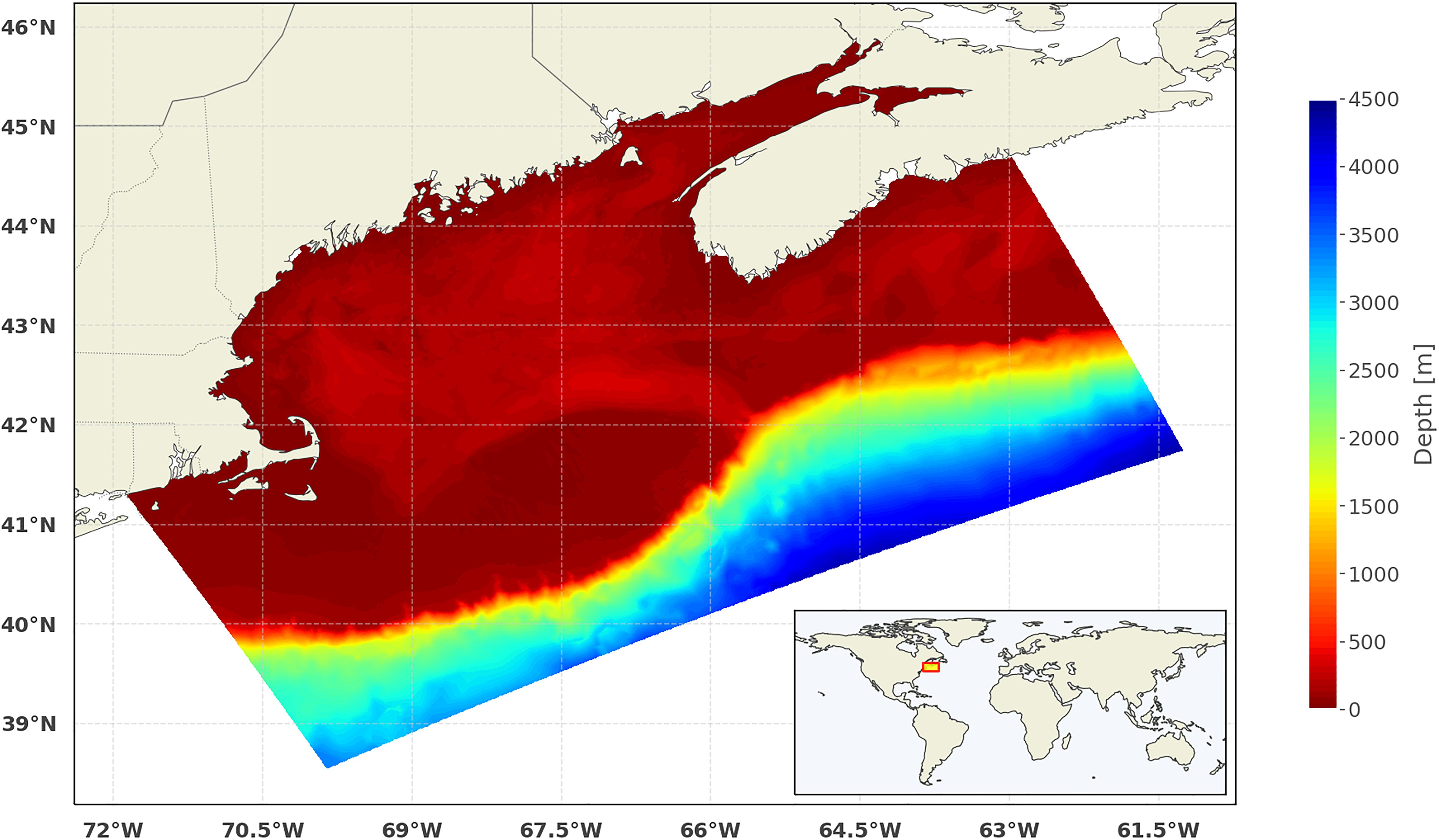
Figure 1. Map of the Gulf of Maine region with the GoMOFS model domain represented using its bathymetric coverage (in meters). The inset shows (with a red-framed yellow rectangle) the location of the model in the world.

Before becoming operational in 2018, the GoMOFS outputs were compared against observations (for the year of 2012) at various depths, and the results demonstrated that the hindcast performance meets the NOS standard criteria (Hess et al., 2003; Zhang et al., 2006). Based on Yang et al. (2016), the following root-mean-squared errors were estimated: less than 1.5°C for temperature, and less than 1.5 psu for salinity. Furthermore, the model successfully reproduced both the magnitude and the annual cycle of the temperature, while it was noted that it tends to overestimate the salinity (Yang et al., 2016).

GoMOFS is run four times per day at 0, 6, 12, and 18 Coordinated Universal Time (UTC) and consists of both a now cast cycle and a forecast cycle. GoMOFS’ nowcast cycle is forced by very-short-range meteorological forecast guidance from the National Weather Service’s (NWS) North American Mesoscale (NAM) weather prediction forecast modeling system (NOS, 2017). GoMOFS’ lateral open ocean boundary conditions for water temperatures, salinity, baroclinic velocity, and sub-tidal water levels are based on predictions from NWS’ Global Real-Time Ocean Forecast System (Global RTOFS) (Peng et al., 2018). Tidal forcing is provided by the ADCIRC Tidal Database (Luettich et al., 1992). Freshwater water inputs, as represented by discharge rates are specified for nine rivers based on the latest observations from United States Geological Survey (USGS) river gages. Each nowcast cycle uses the nowcast from the previous cycle as its initial conditions. There is no data assimilation by GoMOFS (NOAA, 2019b). GoMOFS’ forecast cycle is forced by forecast guidance out to 72 h from the NAM forecast modeling system and Global RTOFS along with tidal forcing from the ADCIRC Tidal Database (NOS, 2017). River discharge rates at the nine river gages for the 72-hour duration of the forecast cycle are not presently based on forecast guidance from a river model forecast modeling system. Instead, the most recent discharge observations at the gages are persisted for the duration of the forecast cycle (Peng et al., 2018). The forecast cycle uses the most recent nowcast to provide its initial conditions (NOAA, 2019b). GoMOFS is run on NOAA Weather and Climate Operational Supercomputer System.

The two GoMOFS variables used in this study are water temperature and salinity. They represent the key components in calculating “synthetic” sound speed profiles from the GoMOFS products. Specifically, the variation of sound speed with depths was calculated – with the related limitations and accuracy – using the dependences of temperature, salinity, and pressure on depth as defined by the United Nations Educational, Scientific and Cultural Organization (UNESCO) adopted equation of Chen and Millero (1977).

Study Area and Input Dataset

The input dataset for this study was collected as ancillary data from a high-resolution hydrographic survey completed during June 2019. The primary objective of the survey was to meet the academic requirements of the Hydrographic Field Course, part of the Ocean Mapping curricula at the University of New Hampshire’s (UNH) Center for Coastal and Ocean Mapping (CCOM). The survey data were collected (and the deliverables were prepared) following the requirements of the NOAA NOS Hydrographic Survey Specifications and Deliverables 2019 (HSSD) manual (NOAA, 2019a). Two distinct areas were surveyed: a main area (hereafter, “A”) that was north of Gerrish Island, ME and south of the Cape Neddick lighthouse; and an offshore area (hereafter, “B”) south east of the coastline around York Harbor (see Figure 2). As shown in the inset of Figure 2, the study area is located in the middle of the western area of the GoMOFS domain region.

FIGURE 2

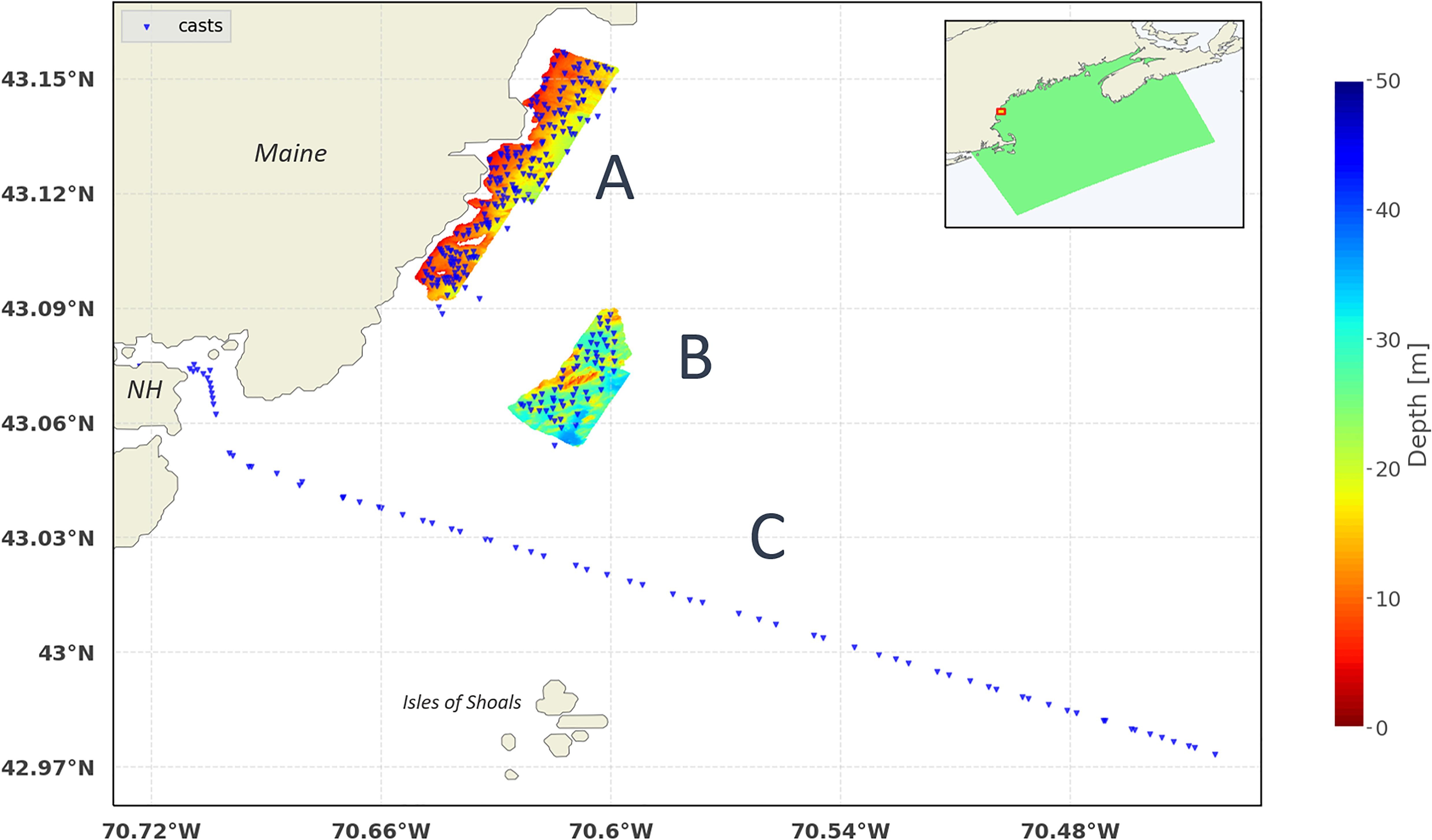
Figure 2. Bathymetric coverage completed by the UNH Hydrographic Field Course 2019. The collected casts (in blue) were grouped into three subsets: the “A” and “B” subsets corresponds to the two distinct surveyed areas, the “C” subset was collected during an offshore-sailing transect. The inset shows the locations of the survey area (red-framed yellow rectangle) and the GoMOFS domain (green tilted rectangle) in the Gulf of Maine.

During the survey, water column properties were measured using an AML Oceanographic MVP30 underway profiler installed onboard the R/V Gulf Surveyor. The towed body was equipped with an AML Sound Velocity, Pressure, and Temperature (SVPT) sensor. At the survey speed of 6–8 knots, the underway profiler can collect profiles up to a depth of about 60 meters, with cycles between 2.0 and 1.8 min. Accordingly, the sampling intervals adopted during the survey were of the order of a few minutes. Such high-rate datasets are useful for the near-continuous evaluation of the structure of the water column below the survey vessel. A data set of 329 casts was acquired during the survey (Figure 2). For the purpose of this study, three subsets where extracted from the whole dataset: the “A” and “B” subsets corresponds to the two distinct surveyed areas, the “C” subset was collected during an offshore-sailing transect (Figure 2). Additional details about the subsets are provided in Table 1 and, graphically, in Figure 3.

TABLE 1

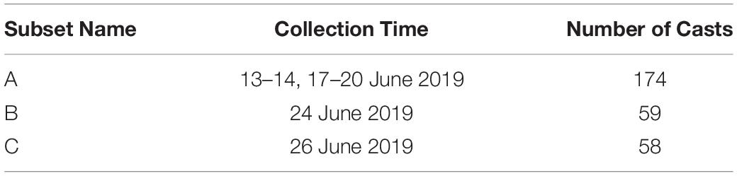
Table 1. Information about the adopted cast subsets.

FIGURE 3

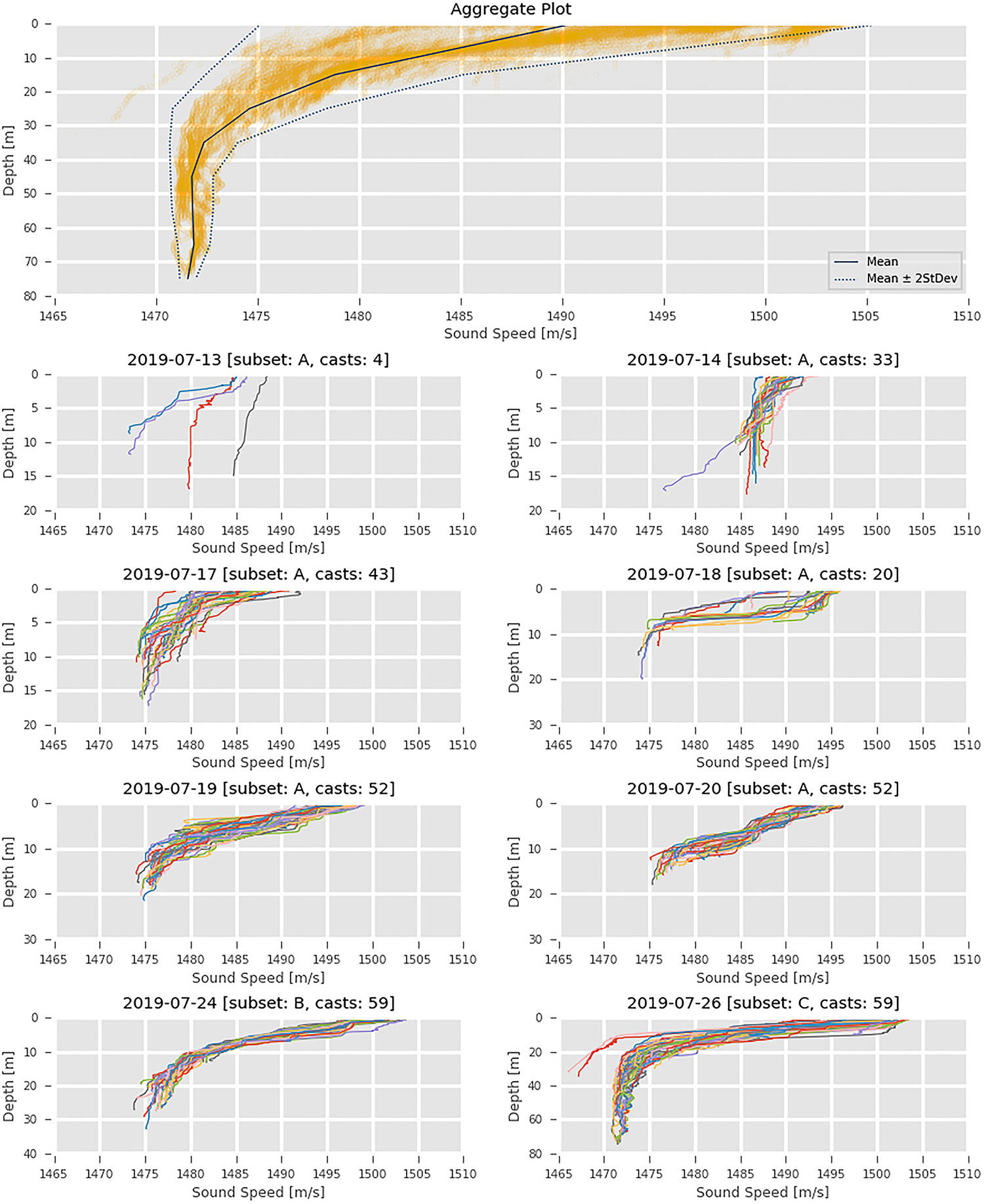
Figure 3. The upper panel shows the aggregate plot based on all the available casts (with the resulting average profile in blue). The other panels show the casts by subset and day of acquisition.

The Sound Speed Manager Application

Jointly developed by the NOAA Office of Coast Survey (OCS) and the UNH’s COM, Sound Speed Manager (SSM) is an open-source application (and software library) designed to perform accurate processing and management of sound speed profiles (HydrOffice, 2019b). Since its inception, the main aim has been to support the surveyors in fulfilling the accuracy and validity requirements of a modern survey workflow (Masetti et al., 2017). After its official deployment during the 2017 NOAA OCS field season, SSM has been adopted by several NOAA and UNOLS vessels, as well as by a number of professionals around the world (Johnson et al., 2018; Masetti et al., 2019; Sowers et al., 2019).

SSM supports cast data collected from various types of devices (e.g., CTDs, velocimeters, expendable bathythermographs (XBT), underway profilers), and formats. Once imported (or received from the network), the user is able to enhance/extend the profile (e.g., based on oceanographic atlases) and then export the validated data in a number of formats commonly recognized by acquisition and processing applications. Through SSM, the surveyor may also retrieve synthetic profiles from oceanographic databases (e.g., the NOAA World Ocean Atlas 2013) and forecast modeling systems (e.g., the NCEP Global Real-Time Forecast System) (Mehra and Rivin, 2010; Levitus et al., 2013). As part of the research efforts presented in this study, SSM was extended to support predictions from NOAA NOS regional operational forecast modeling systems and, specifically, the GoMOFS (Yang et al., 2016). The synthetic profiles from the model forecasts can be used to complement collected profiles with environment variables that have not been directly measured (e.g., the salinity for XBT profiles), extend them to a deeper depth, and/or perform a visual comparison to confirm their reliability.

SSM stores the processed profiles in a per-project SQLite database and provides several analysis functions and tools to manage the database-stored profiles (Masetti et al., 2017). Among those functionalities, the surveyor also has access to a software implementation of the previously cited CastTime algorithm designed to estimate the time when performing the next cast (Wilson et al., 2013).

SmartMap

SmartMap is a tool that estimates the ray-traced refraction component of the surveyed depth uncertainty based on a spatial variability analysis of publicly available oceanographic environmental data (Masetti et al., 2018). First, the SmartMap analysis estimates the uncertainty up to the minimum common depth among the retrieved synthetic profiles. Then, based on the consideration that the largest sound speed variability is commonly observed in the uppermost area of the water column (Medwin and Clay, 1998; Kinsler et al., 2000), the results are provided as a percentage of ray-tracing depth uncertainty ($PD{U}_{r,c}^{rt}$) as a function of the calculated uncertainty (${\mathrm{\delta }}_{r,c}^{rt}$) scaled to the 95% confidence level and the full depth (d_r,c) at each grid location (r,c):

$$PD{U}_{r,c}^{rt}=\frac{2{\mathrm{\delta }}_{r,c}^{rt}}{d_{r,c}}*100.0(1)$$

Finally, a logarithmic transformation is applied (due to the large range of the resulting ray-tracing uncertainty values), and the resulting map is stored in the GeoTIFF format (Ritter and Ruth, 1997). SmartMap maps are made available daily (and stored) through Open Geospatial Consortium (OGC) web services and a Web GIS¹ (Michaelis and Ames, 2012; HydrOffice, 2019a).

SmartMap outputs can be used in all the phases of a survey: planning (e.g., by accessing the output based on the model forecasts), execution (by providing a synoptic representation of the water column variability during the data acquisition), and processing (by retrieving the analysis from past dates) (de Moustier, 2001; Hughes Clarke, 2003; Beaudoin et al., 2004).

The original implementation of SmartMap provides maps based on the predictions from Global RTOFS and data from NOAA World Ocean Atlas 2013 (Mehra and Rivin, 2010; Levitus et al., 2013). Support for GoMOFS forecasts (Yang et al., 2016) has been added to SmartMap (see Figure 4) to underpin the predictive component of the ForeCast algorithm (more details on the algorithm are provided in section “The ForeCast Algorithm”), and ease its potential future transition to operations.

FIGURE 4

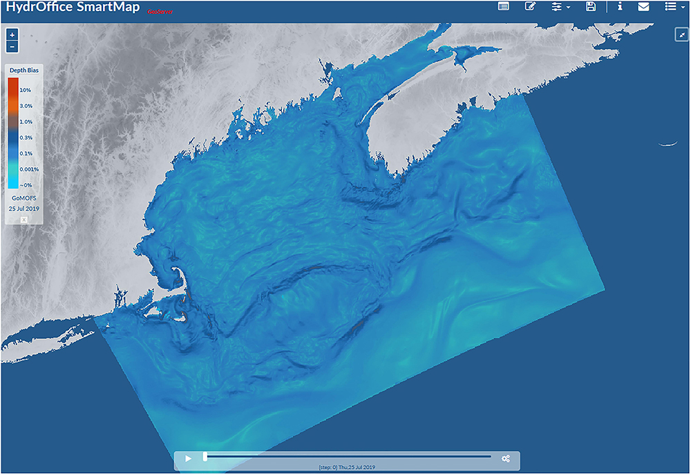
Figure 4. Visualization on the SmartMap Web GIS (https://www.hydroffice.org/smartmap/) of the GoMOFS-based 24-hr forecast map of estimated ray-tracing depth bias as percentage of water depth (valid on July 25, 2019).

The ForeCast Algorithm

The ForeCast algorithm estimates the optimal cast timing by combining a reactive component based on the observed variability and the predicted spatio-temporal variability provided by the predictions of an oceanographic forecast modeling system (i.e., the GoMOFS).

The main processing steps of the algorithm are:

• Application of a constant-gradient ray-tracing algorithm for each newly acquired sound speed profile.

• Using uncertainty analysis, comparison of each newly collected cast with the latest acquired profiles.

• Retrieval of the local GoMOFS-derived spatio-temporal depth bias from the SmartMap WCS.

• Estimation of a new sampling interval based on previous intervals, the GoMOFS-derived spatio-temporal depth bias, and a specified maximum allowable tolerance.

Figure 5 provides a flowchart outlining the main algorithmic steps, data inputs, user parameter, and processing outputs. All the processing steps have been implemented in the Python 3 programming language (van Rossum, 2018).

FIGURE 5

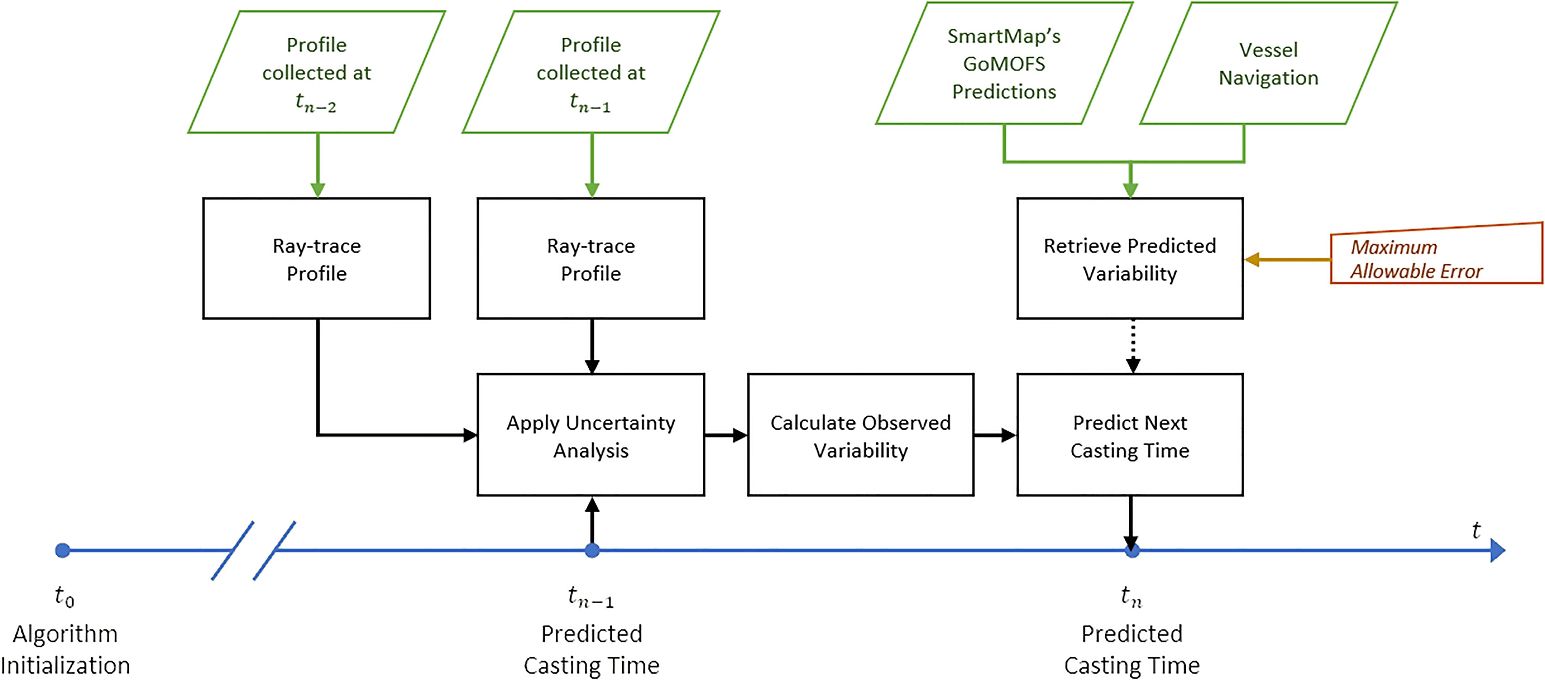
Figure 5. The flowchart shows, in black, the main steps of the ForeCast algorithm with a dashed connector when optional (i.e., the predictive component based on SmartMap’s GoMOFS maps). The inputs are represented in green, the user parameter in orange, and the timeline in blue.

Constant-Gradient Ray-Tracing

Normally, a multibeam echosounder (MBES) repeatedly emits acoustic pulses that are much broader in the across-track direction than along track. After having traveled through the water column, those pulses insonify a seafloor area that usually has a width of several times the measured depth and are then scattered back in multiple directions (Lurton, 2010). The component of each pulse returned to the MBES is processed through electronic beam steering to determine the travel time at each beam angle (Burdic, 1991). Finally, those pairs of travel time and beam angles (β) are combined with the sound speed profile to obtain seafloor depth measurements (z) or the range of mid-water targets within the swath (Medwin and Clay, 1998).

Ray-tracing is one of the most popular methods for obtaining the swath measurements through modeling of underwater sound propagation (Huang, 2012). Ray-tracing is performed by splitting the sound speed profile, c(z), into a set (N) of finite layers (with indices n = 0,…,N), and then calculating the refraction of a ray path across the layer (Medwin and Clay, 1998). With the constant-gradient approach, the ray-tracing algorithm assumes linear variation of sound speed between each subsequent pair of samples in a profile (Medwin and Clay, 1998). For each of the N-1 finite layers, a constant gradient of sound speed (g_n) is estimated:

$$g_n=\frac{c_n-c_{n-1}}{z_n-z_{n-1}}(2)$$

The algorithm then applies the Snell-Descartes law for isotropic media to trace the ray (a is a constant known as the ray parameter):

$$\frac{\cos {\mathrm{\beta }}_n}{c_n}=\frac{\cos {\mathrm{\beta }}_{n-1}}{c_{n-1}}=a(3)$$

The resulting path through the finite layer draws an arc of a circle (see Figure 6) whose center lies at a baseline depth calculated by extrapolating the layer sound speed to zero (Medwin and Clay, 1998). After having calculated the local radius of curvature (R_n), the circular refraction formulae for changes in depths and horizontal ranges (r) can be derived (Lurton, 2010):

FIGURE 6

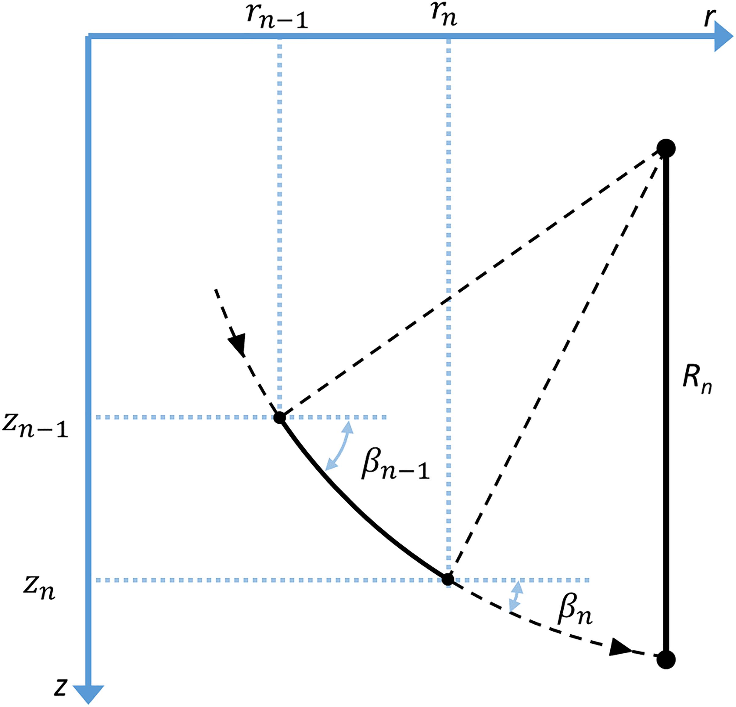
Figure 6. Geometry and symbols used in the constant gradient ray-tracing algorithm for a given ray in a finite layer.

$$R_n=\frac{c_{n-1}}{g_n\cos {\mathrm{\beta }}_{n-1}}(4)$$

$$\{\begin{array}{c}\hfill r_n-r_{n-1}=\frac{c_{n-1}}{g_n\cos {\mathrm{\beta }}_{n-1}}\left(\sin {\mathrm{\beta }}_{n-1}-\sin {\mathrm{\beta }}_n\right)\hfill \\ \hfill z_n-z_{n-1}=\frac{c_{n-1}}{g_n\cos {\mathrm{\beta }}_{n-1}}\left(\cos {\mathrm{\beta }}_n-\cos {\mathrm{\beta }}_{n-1}\right)\hfill \end{array}(5)$$

Finally, the total travel time can be obtained by integration of the travel times along the layers. Figure 7 shows an example of the described ray-tracing algorithm in action, at different initial beam angles.

FIGURE 7

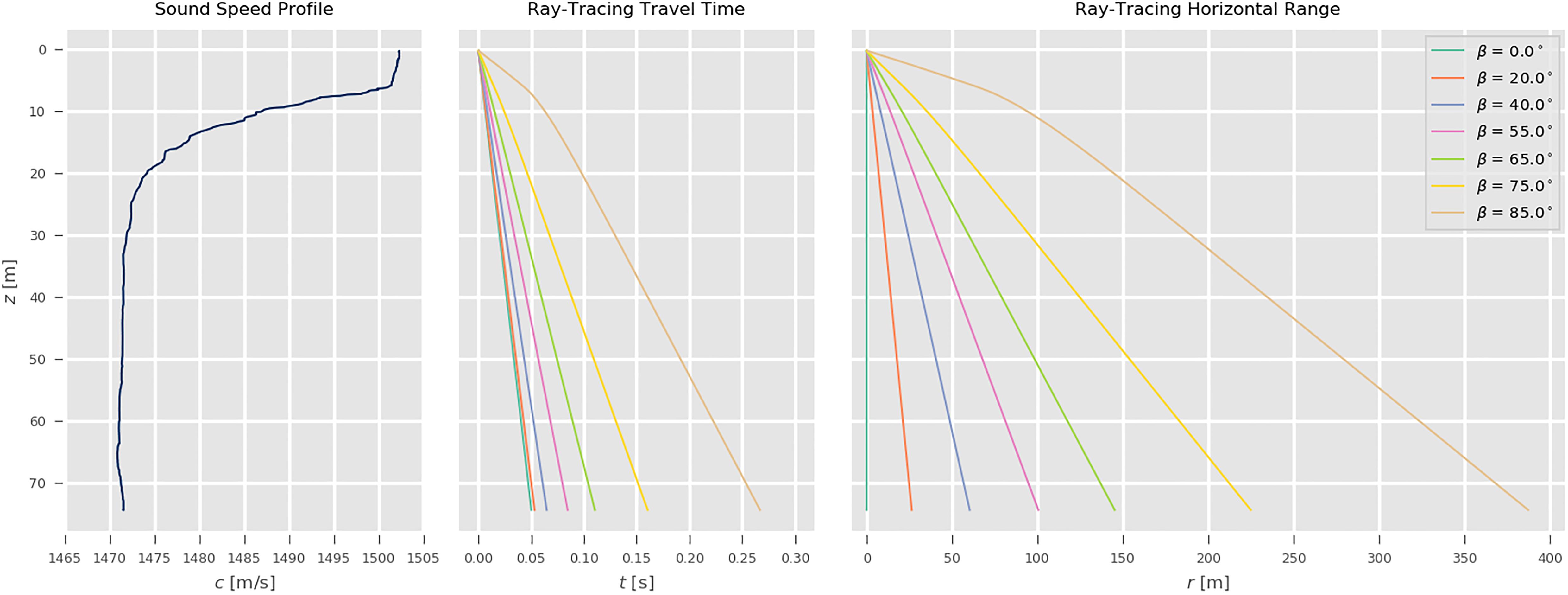
Figure 7. An example of application of the constant gradient ray-tracing algorithm. The left panel shows the sound speed samples (in blues) from one of the collected survey profiles. The middle panel and the right panel, respectively provide the resulting travel time (t) and horizontal range (r) at different initial beam angle (β).

Uncertainty Analysis on Acquired Profiles

The uncertainty analysis adopted by ForeCast is based on pairs of ray-traced profiles (Figure 5). For each profile, the ray-tracing algorithm is iteratively executed until the desired end-point is reached. The depth and launch angle of each individual ray-trace have to be adjusted based on the current sonar configuration: the dynamic draft of the sonar head, the sound speed values measured at the transducer, and the adopted angular swath aperture. The results are interpolated to a decimetric resolution by applying a spline interpolation of third order and stored into a look-up table (Ferguson, 1964). Because sound speed measurements within a given profile are likely collected at depths distinct from another profile, the interpolated values are used to obtain a consistent comparison between pairs of ray-traced sound speed profiles. Since the results of the ray-tracing are symmetrical about the sonar nadir, the computation is only necessary on one side of the sonar swath.

Any bias in the environmental characterization in one or more of the profile layers directly affects the quality of the resulting sonar solutions. As such, by ray-tracing subsequent profiles, it is possible to compare the outdated water column characterization with a newer (and likely better) representation. The ray-tracing outputs can be used to perform a quantitative comparison between pairs of sound speed profiles to estimate the sounding uncertainty due to water column variability. Such an evaluation does not require actual sounding data, and can be performed at any desired depth that is covered by both the profiles (Beaudoin, 2010; Wilson et al., 2013).

Figure 8A shows an example of applying the described uncertainty analysis on two acquired profiles. When profile b is acquired, it is assumed to provide a better representation of the water column conditions than profile a. While profile a was showing quite well-mixed conditions (i.e., water temperature and salinity have limited variations), profile b has generally higher sound speed values as well as the presence of a thermocline. An assessment of the biases that would have been introduced by the continued use profile a is performed and shown in the Figure 8B. This assessment is obtained by first calculating, based on profile b, the travel time required by a ray (with a given initial β) to reach a simulated flat seafloor, then retrieving the corresponding r and z values in the ray-traced profile a. The differences between those values and the corresponding ones in profile b provide the absolute (vertical and horizontal) bias (δz and δr). In other words, the rays based on profile a will no longer end at the assumed flat seafloor because the travel times are derived from the ray-tracing of the (assumed) more correct profile b. The resulting artificial curvature of the seafloor is commonly known as refraction smile, and it is usually used by surveyors to qualitatively evaluate the presence of refraction issues. As shown in both the bias plots in Figure 8, the highest values tend to be associated with beam angles larger than 65° (visualized as a red dotted line). Although possible in ideal conditions to acquire MBES data with a swath aperture larger than 65°, such a value will be adopted as a reference value for this work (Hughes Clarke, 2012; Masetti et al., 2018). For example, given the scenario shown in Figure 8, the depth bias using 65° as initial beam angle would be ∼0.38 m at the deepest common depth between the profiles.

FIGURE 8

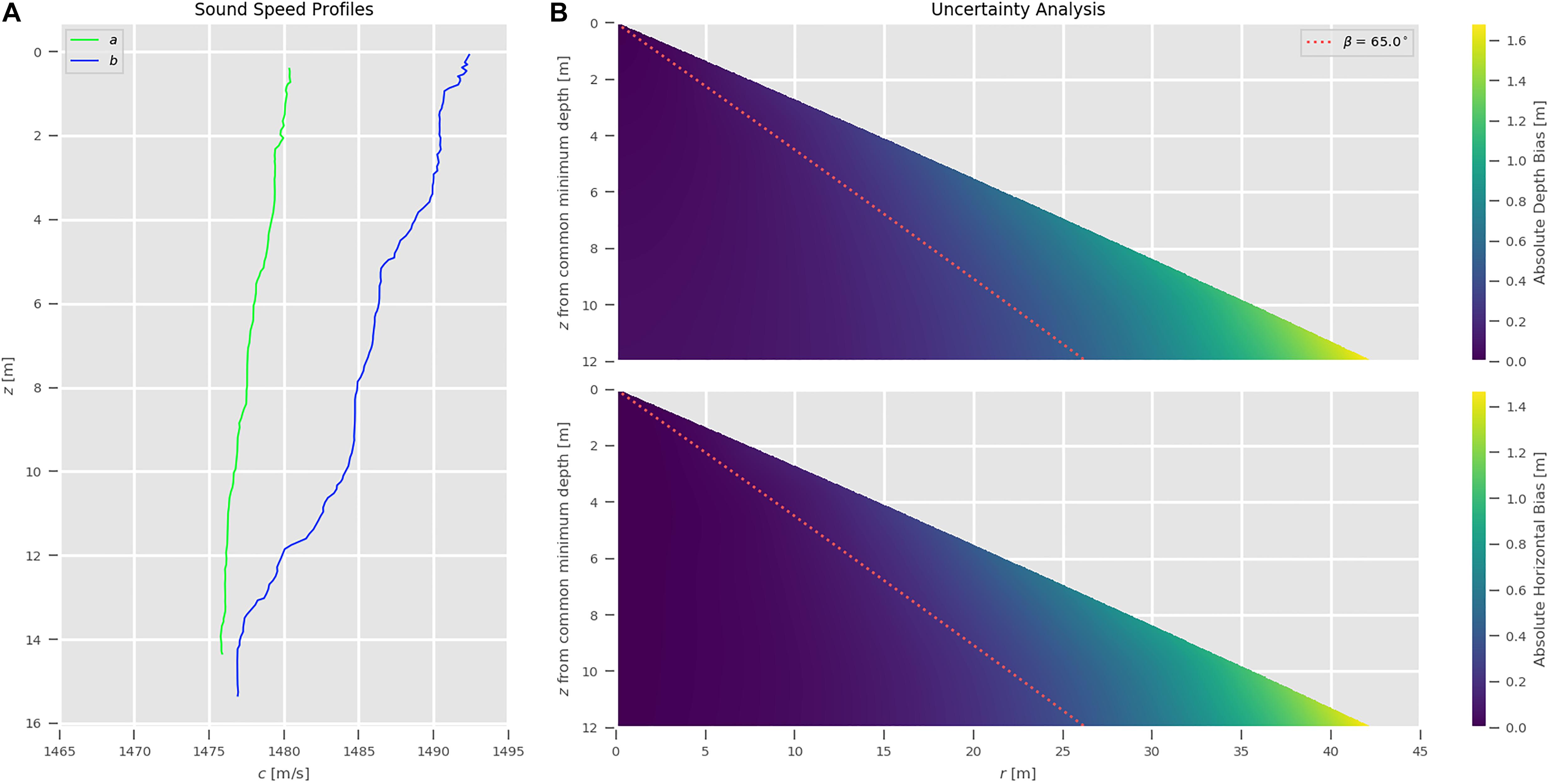
Figure 8. Outcomes from the uncertainty analysis applied to the pair of profiles on the panel (A). The two panels on the right (B) show the absolute depth bias and the absolute horizontal bias, respectively. The initial beam angle of 65° is provided as a reference in dotted red.

Retrieval of the Predicted Spatio-Temporal Variability

The predicted spatio-temporal depth bias for the study area is retrieved through the SmartMap server. As noted in section “SmartMap,” the support for GoMOFS predictions has been added as part of the research efforts of the present study. The main advantage of such a solution is that the download of the large NetCDF files storing the GoMOFS nowcasts and the computationally demanding spatial variability analysis are performed on the remote server (Yang et al., 2016; Masetti et al., 2018). Then, a subset of the map (limited to the survey area, thus usually just a few kilobytes) can be accessed through the GeoServer-provided implementation of the OGC Web Coverage Service (WCS) (Deoliveira, 2008).

Estimation of Future Casting Intervals

The estimation of a new sampling interval is based on a user-specified maximum allowable tolerance that is evaluated against previous intervals and combined with the GoMOFS-derived spatio-temporal depth bias.

Although any error tolerance can be potentially adopted in order to follow agency-specific survey requirements, the default parameters of the ForeCast algorithm are based on the NOAA OCS’s refraction error tolerance (ε_z) for MBES surveys as defined in the HSSD manual (NOAA, 2019a). The ε_z, is given in meters by combining a fixed component and a variable part that is a function of the water depth (wd):

$${\mathrm{\epsilon }}_z=0.3+0.005\times wd(6)$$

The calculated ε_z is useful to provide a baseline (i.e., an upper and a lower limit) of accepted variability surrounding the assumed-correct answer that is derived from ray-tracing the latest profile. Whether the tolerance limits have been exceeded is evaluated at a user-defined β that has to be modified to match the adopted MBES settings. For such an angle, the ForeCast algorithm has a default value of 65° (the assumed outermost beams used and thus the worst-case) that is adopted for the analysis presented in the reminder of this work.

The algorithm logic in estimating the future casting time is based on a target depth bias (δz_tgt) calculated as a percentage of ε_z. The adopted formula for δz_tgt uses the following default value:

$$\mathrm{\delta }{z}_{tgt}=0.5\times {\mathrm{\epsilon }}_z(7)$$

If the analysis is limited to information that can be retrieved from the collected profiles, the solution proposed by Wilson et al. (2013) of assuming that the depth bias linearly increases with the elapsed time between pairs of subsequent profiles would represent an acceptable strategy. However, given that the GoMOFS-based SmartMap maps provide a representation of the oceanographic variability in the survey area, those values are used to derive a spatial component (e.g., a calibration factor) for the ForeCast algorithm, thus potentially improving its forecasting capability (Figure 5). Specifically, the predicted rate of change obtained from the SmartMap analysis is first calibrated using the variability observed in the collected profiles (initialization phase), then the obtained calibration value is used to predict the optimal timing interval based on the δz_tgt (Figure 9). The adoption of such an approach requires the addition of the vessel route and speed over ground to the algorithm’s input parameters that are not required in the CastTime algorithm (Wilson et al., 2013). However, when a model forecast is not available, the ForeCast algorithm reverts back to the reactive-only method (see Figure 9B).

FIGURE 9

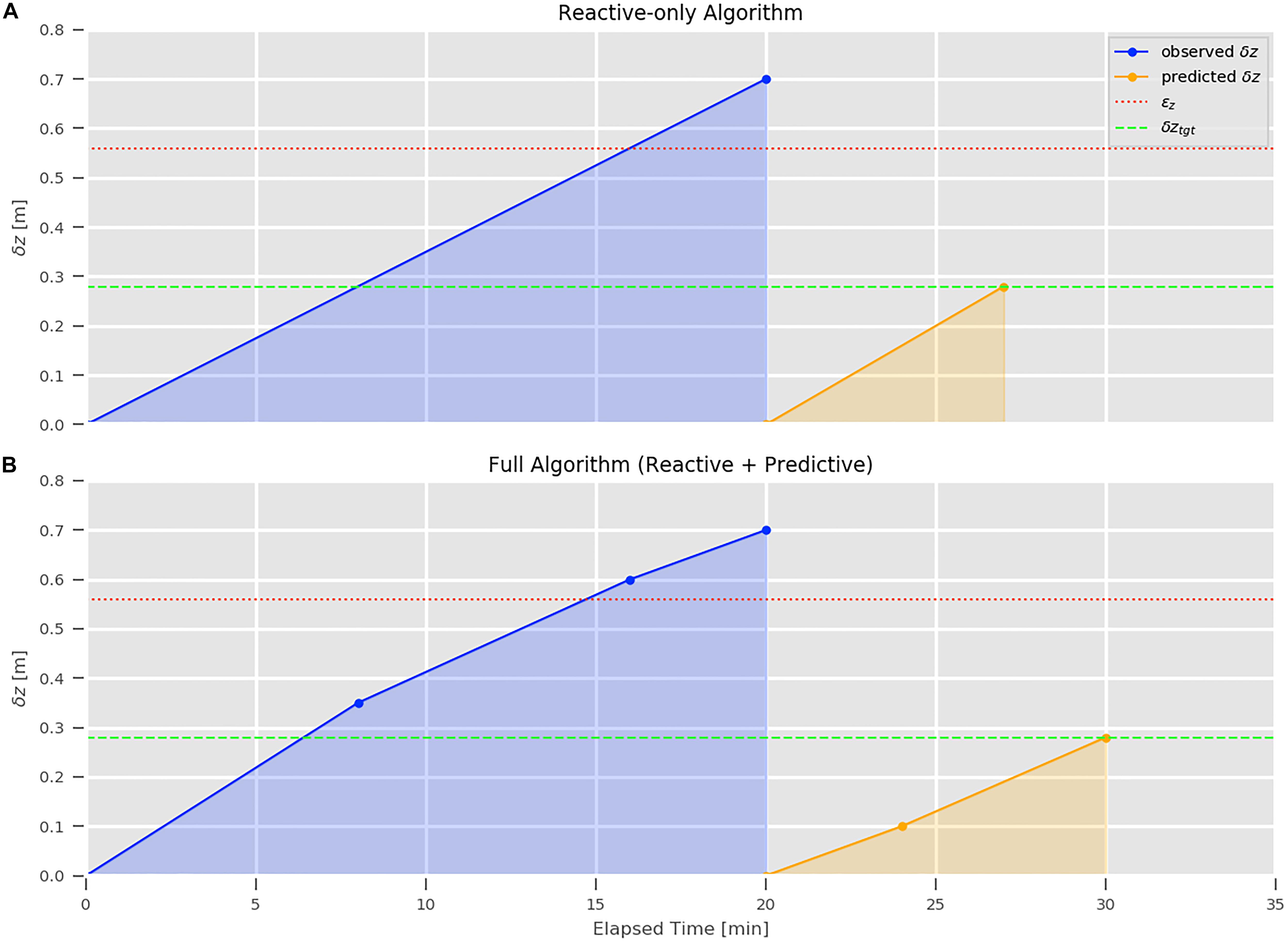
Figure 9. An example of observed variability exceeding the maximum allowable error (red dotted line). When a model forecast is not available, the ForeCast algorithm assumes linear increase in depth bias between observed profile (A). (B) Shows an example application for the full algorithm where the predictive component (based on GoMOFS SmartMap maps) is calibrated using the observed spatial variability at different model locations along the track (in blue) and applied to predict the time interval (in orange) when the target depth bias (green dashed line) is reached.

Results

The testing was conducted using the three subsets (“A”, “B”, and “C”) of profiles described in section “Study Area and Input Dataset.” The profiles, collected in the “s21” variant of the Kongsberg Maritime SSP datagram, have been loaded in SSM, assessed for quality assurance, and then stored in the application’s project SQLite-based database (Kongsberg, 2015).

For each subset, the profiles were used to evaluate the use of the synthetic values derived from the GoMOFS nowcasts in place of the observed data (Figure 10). The percentages of profiles that fulfill the refraction error tolerance (ε_z) and the target depth bias (δz_tgt) are summarized in Figure 11. The maps in Figure 12 are provided to spatially locate the calculated depth biases.

FIGURE 10

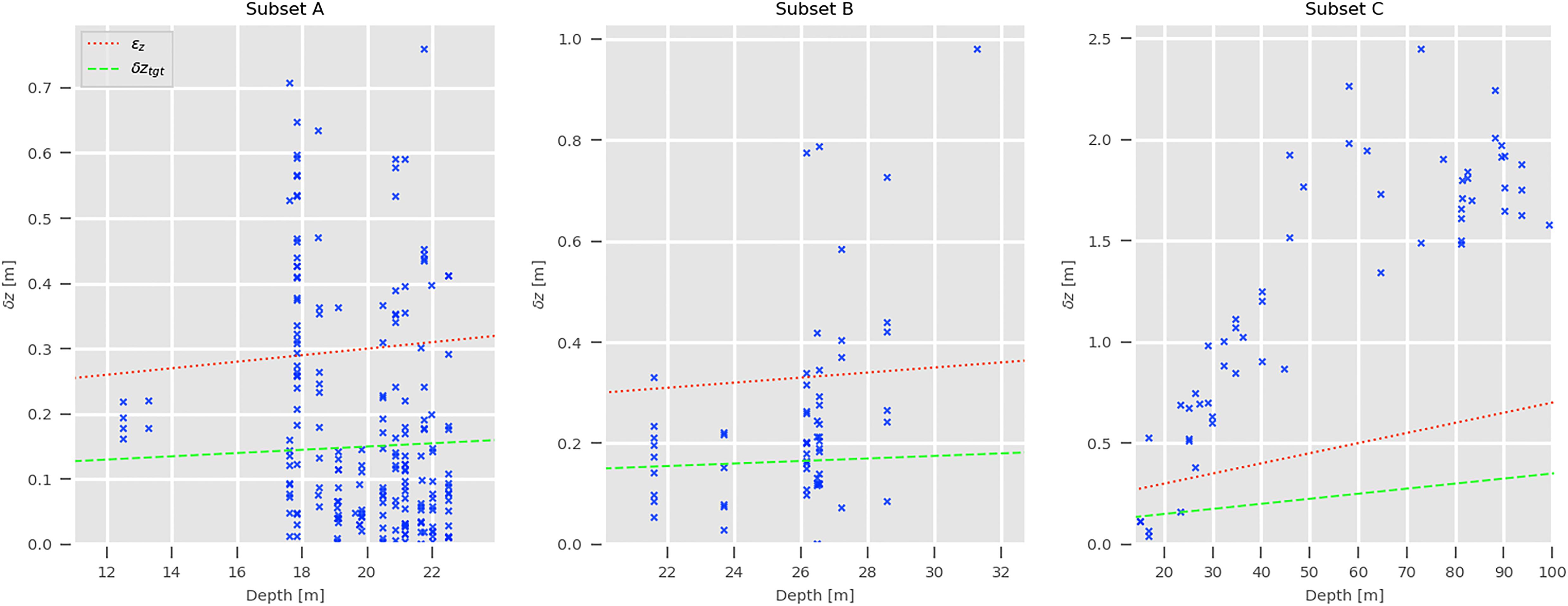
Figure 10. Each collected profile is compared against a synthetic profile retrieved from the GoMOFS predictions. The resulting depth bias (δz) is shown with a blue cross, while the refraction error tolerance (ε_z) and the target depth bias (δz_tgt) are represented by a red dotted line and a green dashed line, respectively.

FIGURE 11

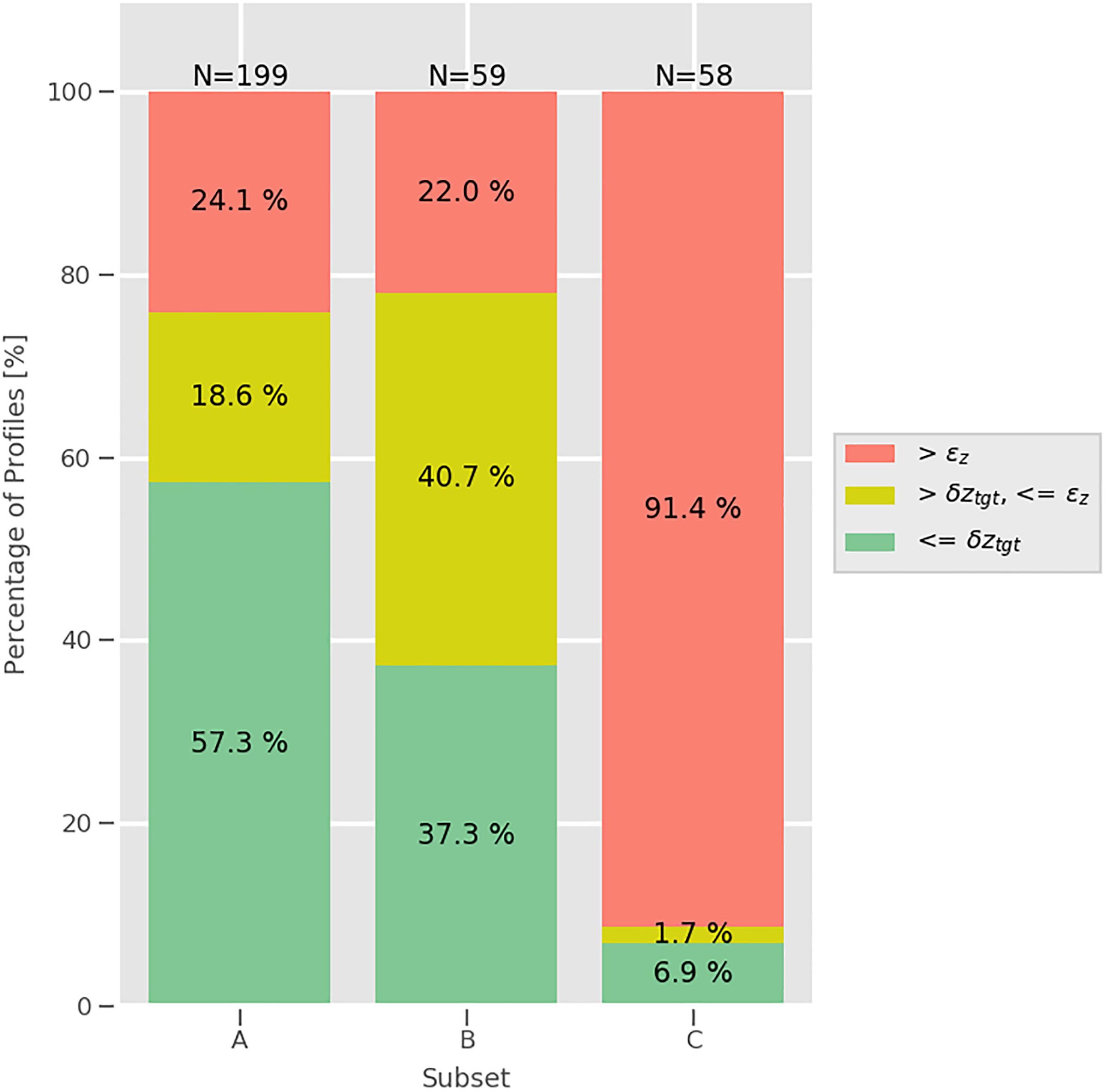
Figure 11. Percentages of GoMOFS-derived profiles per subset that have δz exceeding ε_z (in red), within ε_z and δz_tgt (in yellow), and fulfilling this latter requirements (in green).

FIGURE 12

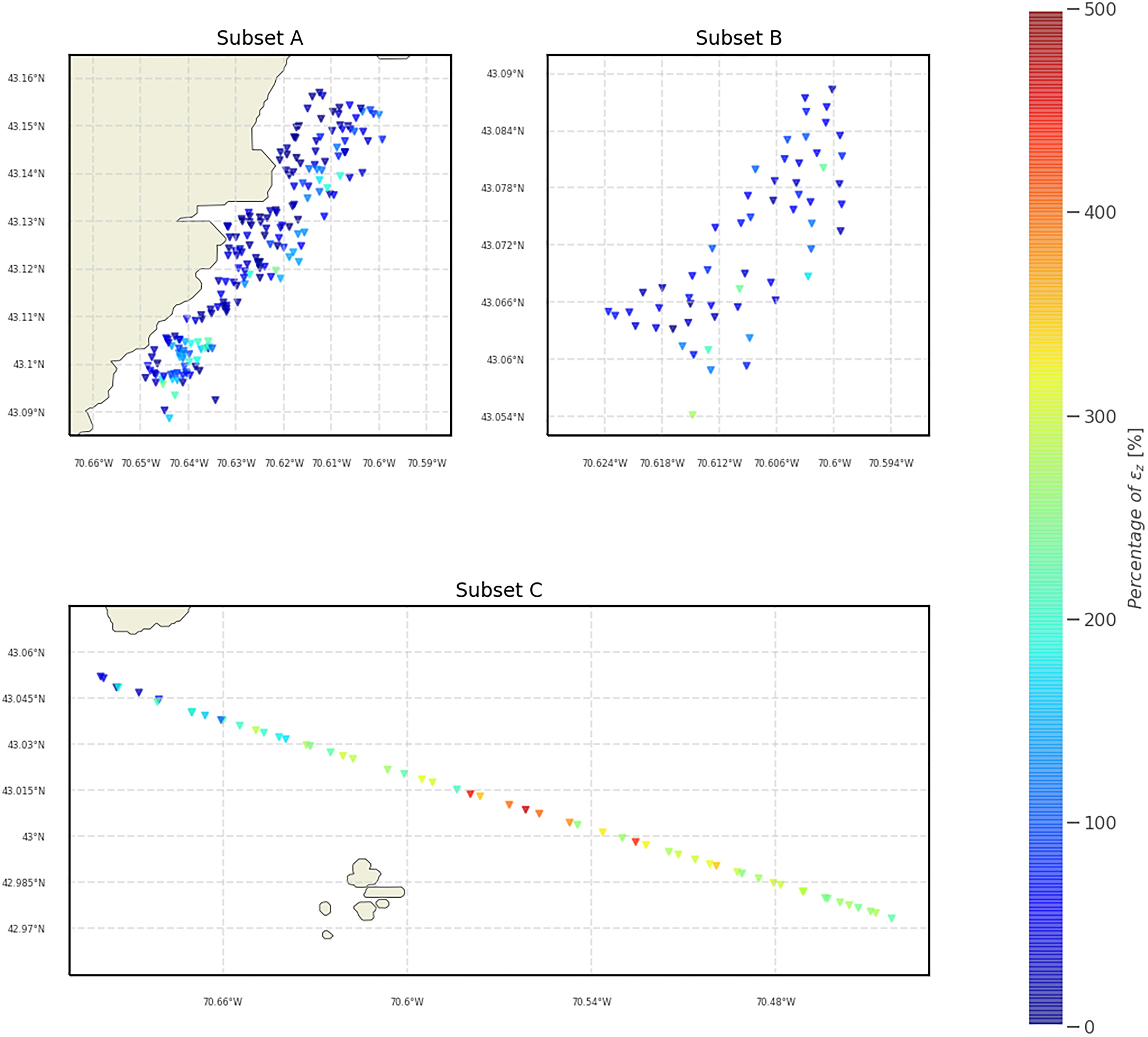
Figure 12. Georeferenced δz derived from comparing observations and GoMOFS-derived synthetic profiles. The values are represented as percentage of ε_z.

Due to the higher variability in depth bias, the profiles in subset C were selected to evaluate the ForeCast algorithm. The profiles were analyzed separately based on the vessel heading during the data acquisition: seaward (Figure 13) and shoreward (Figure 14).

FIGURE 13

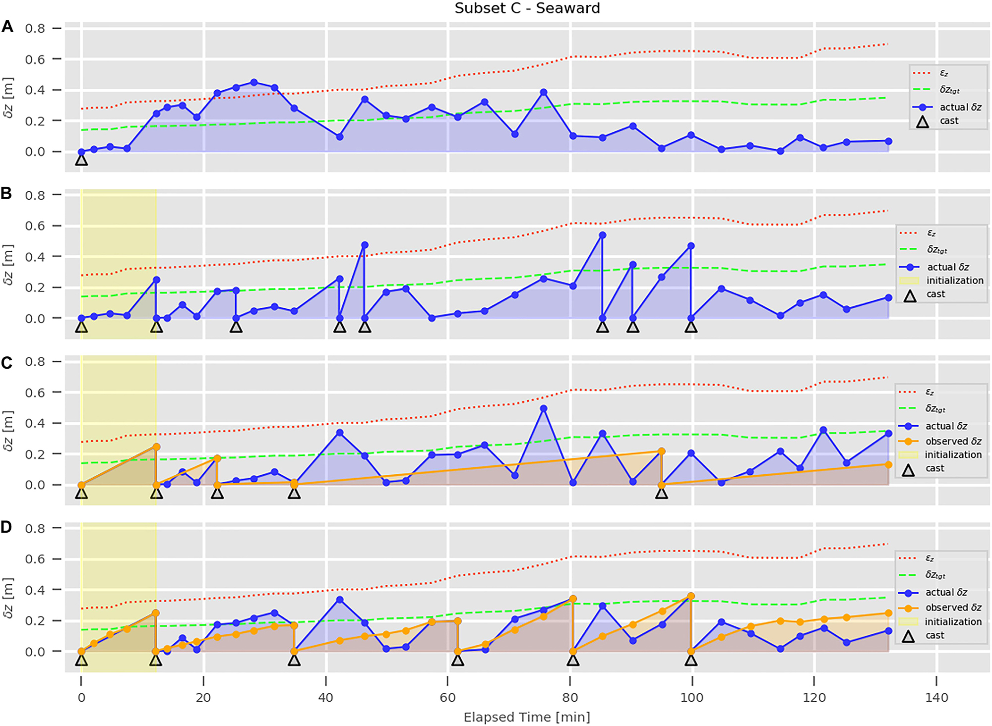
Figure 13. Worst-case scenario (A), optimal solution (B), solutions from the reactive-only (C) and the full (D) ForeCast algorithm for profiles from Subset C collected in the seaward direction.

FIGURE 14

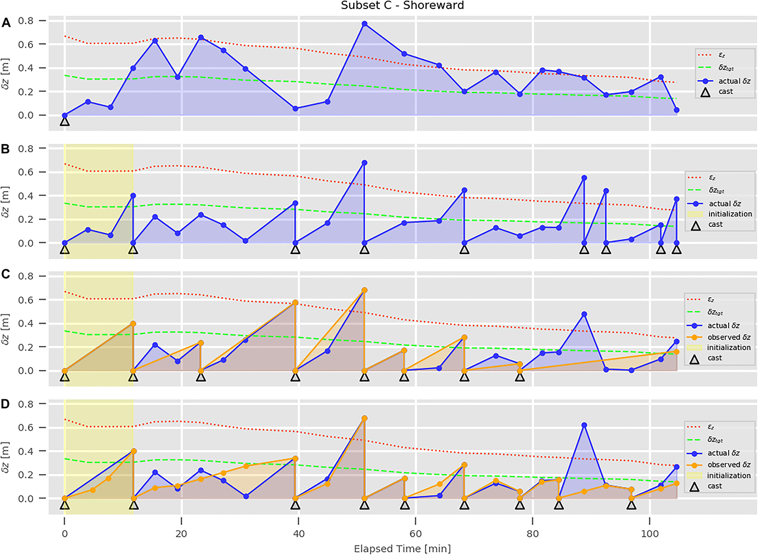
Figure 14. Worst-case scenario (A), optimal solution (B), solutions from the reactive-only (C) and the full (D) ForeCast algorithm for profiles from Subset C collected in the shoreward direction.

In Figures 13A, 14A shows the evolution of δz in the worst-case scenario that only a single cast would have been collected at the beginning of the transect. In Figures 13B, 14B, an optimal cast timing solution is presented. Specifically, based on the assumption that the high-density subset represents an over-sampled water column, the addition of a new cast is triggered each time that δz exceeds the locally estimated δz_tgt. The first obtained cast time is used to define the initialization time (in yellow) of the ForeCast algorithm. The predicted casting times in Figures 13C,D, 14C,D are obtained from the ForeCast algorithm in two different ways: by only using its reactive component (thus, with a logic similar to the CastTime algorithm) in Figures 13C, 14C, and with its full version (thus, adjusting the estimated times based on the spatial component provided by the SmartMap analysis of GoMOFS predictions) in Figures 13D, 14D. The actual δz is the depth bias computed using the full high-density series of profiles (blue markers in Figures 13, 14). The observed δz is the depth bias that would be observed following the cast times suggested by the algorithm (orange markers in Figures 13C,D, 14C,D). For the full ForeCast algorithm, Figures 13D, 14D also shows the intermediate estimated observed δz (i.e., adjusted based on the GoMOFS SmartMap output) as orange dots between cast times (see Figure 9).

The algorithm performances may be assessed by both evaluating the survey efficiency and the mitigation of the resulting refraction-driven depth bias in the acquired soundings. This latter is based on the comparison between the observed δz (in orange) and the actual δz (in blue). δz For instance, in Figure 13D, both the observed δz and the actual δz are assumed zero at the 80-minute epoch; then, the observed δz is increased with time in function of the underline spatial variability predicted by the GoMOFS model. The algorithm triggers the collection of a new profile at the 100-minute epoch, when the observed δz overcomes the target depth bias (δz_tgt) of 0.37 m. The actual δz between the casts suggested by the algorithm are not used in the algorithm computation, but they are provided for evaluation of the uncaptured variability. For instance, there are ∼0.2 m of uncaptured depth bias at the 84-minute epoch in Figure 13D.

Discussion

The use of the GoMOFS-predicted oceanographic variability in the water column in place of the observed profiles was evaluated in Figure 10 for each of the three input subsets. Although the results are quite satisfactory for subsets A and B – with 74.4 and 76.3% of profiles fulfilling the allowable ε_z, respectively (Figure 11) –, the large number of profiles (63.8%) in subset C exceeding ε_z and their values in percentage of ε_z (Figure 12) demonstrate reliability concerns in adopting the model-derived synthetic profiles to fully substitute the profile collection during a regular survey. Indeed, the critical hydrographic practice of collecting hydrocasts should never be abandoned. Nevertheless, the GoMOFS-derived synthetic profiles (in conjunction with synthetic profiles derived from climatological atlases such as WOA) provide a useful reference to evaluate the quality of newly collected data (e.g., identifying a malfunctioning device). Furthermore, they offer acceptable estimates to be used to enhance and extend the data collected on-site by sound speed profilers. The accuracy of nowcasts from NOS’ regional oceanographic forecast modeling systems are expected to improve as they are upgraded to assimilate in situ and satellite-based observations. Based on such considerations, both capabilities (visual comparison and profile enhancement) were added to SSM to facilitate the transition from research to operations of some of the outcomes of this study.

The second part of the results presented in this work evaluates whether the uncertainty estimation of the oceanographic variability can be used as a meaningful input to estimate the optimal casting time. The predictive component of the ForeCast algorithm required the addition of a GoMOFS layer to SmartMap (Figure 4). Such an addition does not only represent a required step toward a potential future transition to operations of the ForeCast algorithm, but also provides surveyors mapping in the Gulf of Maine with a tool to synoptically evaluate the spatio-temporal variability of the oceanographic conditions in the survey area.

Figures 13, 14 show the evolution of δz in different scenarios, using the analysis of ray-tracing uncertainty to evaluate the adequacy level at different profiling times. The worst-case scenarios represented in Figures 13A, 14A clearly show the need to perform additional casts after the collection of the first profile. The optimal solutions, represented in Figures 13B, 14B, provide a baseline to evaluate the performance of the reactive-only (Figures 13C, 14C) and the full (Figures 13D, 14D) ForeCast algorithm. The full algorithm estimates cast times whose actual δz values are generally lower than the ones provided by the reactive-only algorithm. Furthermore, a surveyor following the full algorithm would have exceeded the threshold for ε_z in only one case (shoreward case, Figure 14D), while it happens a few times in Figures 14C,D. Based on such considerations, the proposed method seems to alleviate the subjectivity in the determination of the casting interval and improve the overall sounding accuracy for effect of the predicted spatio-temporal variability provided by GoMOFS. However, more extensive test datasets need to be collected to confirm these results, and new data acquisition are planned for the UNH CCOM’s Hydrographic Field Course in 2020. Among others, a relevant possible future improvement to the current algorithm would be in the definition of the initialization time that is currently estimated based on the first obtained cast time from the optimal solution. From a speculative point of view, a relation between the initialization time and the SmartMap-provided $PD{U}_{r,c}^{rt}$ could be identified. Another improvement could be manifested by integrating the values of sound speed continuously measured at the MBES transducer. The weight given to such point measurements is an open research question.

Although a general evaluation of the survey environment can potentially be retrieved directly from the available climatological atlases and forecast modeling systems, the applications presented in this work digest the large amount of information contained in four-dimensional oceanographic variables and present it in a way most relevant to the ocean mapper. A more accurate knowledge of the oceanographic variability in the survey area has several potential implications. For instance, during the planning phase, surveying directions may be oriented to limit the number of crossings of large uncertainty fronts. In case that the estimated uncertainty for the outmost swath depths is too large based on the targeted specifications, the time of survey execution may be modified, or the estimated swath coverage can be reduced accordingly. Other possible uses are the selection of a calibration site with limited environmental variability and the identification of the appropriated device to sample the water column (e.g., a survey area with high environmental variability should suggest the adoption of an underway profiler).

This work presents a shift in awareness from the traditional method of monitoring the sound speed at the transducer – a point measurement of sound speed (at ∼1-Hz temporal resolution) that has a critical role in beam forming – and performing profiles measurements at fixed intervals (with additional casts as needed). The combination of these two types of measurements provide a limited awareness of the surrounding oceanographic variability that the methods presented in this work try to overcome. The adoption of the proposed methods has the potential to improve efficiency in survey operations as well as the quality of resulting ocean mapping products.

Data Availability Statement

The GoMOFS-derived datasets analyzed for this study can be downloaded from the SmartMap server (https://smartmap.ccom. unh.edu/geoserver/web/). The original GoMOFS outputs were retrieved from the NOAA CO-OPS THREDDS server (https://opendap.co-ops.nos.noaa.gov/thredds/catalog.html).

Author Contributions

GM, MS, and LM: conceptualization and project administration. GM and JK: formal analysis. GM, MS, LM, and JK: methodology. GM: writing the original draft. MS, LM, and JK: writing, review, and editing. GM and MS: analyzed the data.

Funding

This work was supported by the National Oceanic and Atmospheric Administration (NOAA) Grant NA15NOS4000200 and the National Science Foundation (NSF) Grant 1524585.

Conflict of Interest

The authors declare that the research was conducted in the absence of any commercial or financial relationships that could be construed as a potential conflict of interest.

Acknowledgments

The authors would like to acknowledge the contribution of Semme Dijkstra, Andrew Armstrong, and the students of the UNH CCOM’s Hydrographic Field Course 2019, for the collected environmental data analyzed in this study; Jason Greenlaw (Earth Resources Technology, NOAA nowCOAST project) and Erin Nagel (University Corporation for Atmospheric Research, NOAA nowCOAST project), for assisting in the retrieval of the regional operational forecast model outputs.

Footnotes

1. ^ https://www.hydroffice.org/smartmap/

References

Bauer, P., Thorpe, A., and Brunet, G. (2015). The quiet revolution of numerical weather prediction. Nature 525, 47–55. doi: 10.1038/nature14956

PubMed Abstract | CrossRef Full Text | Google Scholar

Beaudoin, J. (2010). Real-time monitoring of uncertainty due to refraction in multibeam echo sounding. Hydrogr. J. 134, 3–13.

Google Scholar

Beaudoin, J., Hughes Clarke, J., and Bartlett, J. (2004). Application of surface sound speed measurements in post-processing for multi-sector multibeam echosounders. Int. Hydrogr. Rev. 5, 26–31.

Google Scholar

Beaudoin, J., Kelley, J. G., Greenlaw, J., Beduhn, T., and Greenaway, S. F. (2013). “Oceanographic weather maps: using oceanographic models to improve seabed mapping planning and acquisition,” in US Hydro 2013 (New Orleans, LA).

Google Scholar

Burdic, W. S. (1991). Underwater Acoustic System Analysis. New Jersey: Prentice Hall.

Google Scholar

Chen, C. T., and Millero, F. J. (1977). Speed of sound in seawater at high pressures. J. Acoust. Soc. Am. 62, 1129–1135. doi: 10.1121/1.381646

PubMed Abstract | CrossRef Full Text | Google Scholar

de Moustier, C. (2001). “Field evaluation of sounding accuracy in deep water multibeam swath bathymetry,” in OCEANS, 2001. MTS/IEEE Conference and Exhibition (Piscataway, NJ: : IEEE), 1761–1765.

Google Scholar

Deoliveira, J. (2008). “GeoServer: uniting the GeoWeb and spatial data infrastructures,” in 10th International Conference for Spatial Data Infrastructure, (St. Augustine).

Google Scholar

Dudhia, J. (2014). A history of mesoscale model development. AsiaPacific. J. Atmos. Sci. 50, 121–131. doi: 10.1007/s13143-014-0031-8

CrossRef Full Text | Google Scholar

Ferguson, J. (1964). Multivariable curve interpolation. J. ACM 11, 221–228. doi: 10.1145/321217.321225

PubMed Abstract | CrossRef Full Text | Google Scholar

Furlong, A., Osler, J., Christian, H., Cunningham, D., and Pecknold, S. (2006). “The moving vessel profiler (MVP)-a rapid environmental assessment tool for the collection of water column profiles and sediment classification,” in Proceedings of the Undersea Defence Technology Pacific Conference 2006 (San Diego, CA), 1–13.

Google Scholar

Greenberg, D. A. (1979). A numerical model investigation of tidal phenomena in the bay of fundy and gulf of maine. Mar. Geod. 2, 161–187. doi: 10.1080/15210607909379345

CrossRef Full Text | Google Scholar

Hess, K. W., Gross, T. F., Schmalz, R. A., Kelley, J. G. W., Aikman, F., Wei, E., et al. (2003). NOAA Technical Report NOS CS 17: NOS Standards for Evaluating Operational Nowcast and Forecast Hydrodynamic Model Systems. Silver Spring, MD: National Oceanic and Atmospheric Administration.

Google Scholar

Huang, X. (2012). A comprehensive study of the Bellhop algorithm for underwater acoustic channel modelings. J. t Acous. Soc. Am. 132, 1942–1942. doi: 10.1121/1.4755149

CrossRef Full Text | Google Scholar

Hughes Clarke, J., Lamplugh, M., and Kammerer, E. (2000). “Integration of near-continuous sound speed profile information,” in Proceedings of Canadian Hydrographic Conference 2000 (Canada).

Google Scholar

Hughes Clarke, J. E. (2003). Dynamic motion residuals in swatch sonar data: ironing out the creases. Int. Hydrogr. Rev. 4, 6–23.

Google Scholar

Hughes Clarke, J. E. (2012). “Optimal use of multibeam technology in the study of shelf morphodynamics,” in Sediments, Morphology and Sedimentary Processes on Continental Shelves: Advances in Technologies, Research and Applications, eds M. Z. Li, C. R. Sherwood, and P. R. Hill (Hoboken, NJ: John Wiley & Sons), 440.

Google Scholar

Hughes Clarke, J. E. (2018). The impact of acoustic imaging geometry on the fidelity of seabed bathymetric models. Geosciences 8:109. doi: 10.3390/geosciences8040109

CrossRef Full Text | Google Scholar

Hughes Clarke, J. E., Hiroji, A., Rice, G., Sacchetti, F., and Quinlan, V. (2017). Regional seabed backscatter mapping using multiple frequencies. J. Acous,. Soc. Am. 141, 3948–3948. doi: 10.1121/1.4988963

CrossRef Full Text | Google Scholar

HydrOffice, (2019a). SmartMap. Smart map the world!. Available: https://www.hydroffice.org/smartmap/main (accessed 24 July 2019).

Google Scholar

HydrOffice, (2019b). Sound Speed Manager. Ease the management of your profiles!. Available: https://www.hydroffice.org/soundspeed (accessed 24 July 2019).

Google Scholar

IHO (2011). C-13: Manual Of Hydrography, 1.04 Edn. Monaco: International Hydrographic Organization.

Google Scholar

Johnson, P., Ferrini, V. L., Jerram, K., and Masetti, G. (2018). “Multibeam advisory committee: looking back on seven years of multibeam echosounder system acceptance and quality assurance testing for the ships of the U.S. Academic Fleet,” in Femme 2018 (Bordeaux).

Google Scholar

Kinsler, L. E., Frey, A. R., Coppens, A. B., and Sanders, J. V. (2000). Fundamentals of Acoustics. New York, NY: Wiley.

Google Scholar

Kongsberg. (2015). EM Series Datagram Formats - Instruction Manual - rev.U. Norway: Kongsberg Maritime AS.

Google Scholar

Lamarche, G., and Lurton, X. (2018). Recommendations for improved and coherent acquisition and processing of backscatter data from seafloor-mapping sonars. Mar. Geophys. Res. 39, 5–22. doi: 10.1007/s11001-017-9315-6

CrossRef Full Text | Google Scholar

Lecours, V., Devillers, R., Schneider, D. C., Lucieer, V. L., Brown, C. J., and Edinger, E. N. (2015). Spatial scale and geographic context in benthic habitat mapping: review and future directions. Mar,. Ecol. Progr. Ser. 535, 259–284. doi: 10.3354/meps11378

CrossRef Full Text | Google Scholar

Levitus, S., Antonov, J., Baranova, O. K., Boyer, T., Coleman, C., Garcia, H., et al. (2013). The world ocean database. Data Sci. J. 12, WDS229–WDS234. doi: 10.2481/dsj.WDS-041

CrossRef Full Text | Google Scholar

Lucieer, V., Huang, Z., and Siwabessy, J. (2016). Analyzing uncertainty in multibeam bathymetric data and the impact on derived seafloor attributes. Mar. Geod. 39, 32–52. doi: 10.1080/01490419.2015.1121173

CrossRef Full Text | Google Scholar

Luettich, R. A. Jr., Westerink, J. J., and Scheffner, N. W. (1992). “ADCIRC: an advanced three-dimensional circulation model for shelves, coasts, and estuaries,” in Report 1. Theory and Methodology of ADCIRC-2DDI and ADCIRC-3DL (Vicksburg, MS: Coastal engineering research center).

Google Scholar

Lurton, X. (2010). An Introduction to Underwater Acoustics : Principles and Applications. New York, NY: Springer.

Google Scholar

Lurton, X., Lamarche, G., Brown, C., Lucieer, V., Rice, G., Schimel, A., et al. (2015). “Backscatter measurements by seafloor−mapping sonars: guidelines and recommendations,”in A Collective Report by Members of the GeoHab Backscatter Working Group. (New Zealand) 1–200.

Google Scholar

Malik, M., Lurton, X., and Mayer, L. A. (2018). A framework to quantify uncertainties of seafloor backscatter from swath mapping echosounders. Mar. Geophys. Res. 39, 151–168. doi: 10.1007/s11001-018-9346-7

CrossRef Full Text | Google Scholar

Masetti, G., Faulkes, T., and Calder, B. R. (2019). “Opening the black boxes in ocean mapping: design and implementation of the hydroffice framework,” in AMSA 2019 (Freemantle, WA).

Google Scholar

Masetti, G., Gallagher, B., Calder, B. R., Zhang, C., and Wilson, M. (2017). Sound speed manager: an open-source application to manage sound speed profiles. Int. Hydrogr. Rev. 17, 31–40.

Google Scholar

Masetti, G., Kelley, J. G. W., Johnson, P., and Beaudoin, J. (2018). A Ray-Tracing Uncertainty Estimation Tool For Ocean Mapping. IEEE Access 6, 2136–2144. doi: 10.1109/ACCESS.2017.2781801

CrossRef Full Text | Google Scholar

Mayer, L., Jakobsson, M., Allen, G., Dorschel, B., Falconer, R., Ferrini, V., et al. (2018). The nippon foundation—GEBCO Seabed 2030 Project: the quest to see the world’s oceans completely mapped by 2030. Geosciences 8, 63. doi: 10.3390/geosciences8020063

CrossRef Full Text | Google Scholar

Mayer, L. A. (2014). Ocean mapping. J. Ocean Technol. 9, 13–18.

Google Scholar

Medwin, H., and Clay, C. (1998). Fundamentals of Acoustical Oceanography. Cambridge, MA: Academic Press.

Google Scholar

Mehra, A., and Rivin, I. (2010). A Real Time Ocean Forecast System for the North Atlantic Ocean. Terr. Atmos. Ocean. Sci. 21, 211–218.

Google Scholar

Michaelis, C. D., and Ames, D. P. (2012). Considerations for Implementing OGC WMS and WFS Specifications in a Desktop GIS. J. Geogr. Inform. Syst. 4, 161. doi: 10.4236/jgis.2012.42021

CrossRef Full Text | Google Scholar

Montereale-Gavazzi, G., Roche, M., Degrendele, K., Lurton, X., Terseleer, N., Baeye, M., et al. (2019). Insights into the Short-Term Tidal Variability of Multibeam Backscatter from Field Experiments on Different Seafloor Types. Geosciences 9:34. doi: 10.3390/geosciences9010034

CrossRef Full Text | Google Scholar

NOAA (2019a). Hydrographic Surveys Specifications and Deliverables. Silver Spring, MD: National Oceanic and Atmospheric Administration, National Ocean Service.

Google Scholar

NOAA (2019b). The Gulf of Maine Operational Forecast System (GoMOFS) NOAA Tides and Currents. Silver Spring, MD: NOAA.

Google Scholar

NOS (2017). Updated: Implementation of New Oceanographic Forecast Modeling System for the Gulf of Maine Effective January 3, 2018. NOS Service Change Notice 17-108. Available: https://www.weather.gov/media/notification/pdfs/scn17-108nos_gomofsaaa.pdf (accessed December 4, 2017).

Google Scholar

Peng, M., Zhang, A., and Yang, Z. (2018). “Implementation of the gulf of maine operational forecast system (GOMOFS) and the semioperational nowcast/forecast skill assessment,”in NOAA Technical Report NOS CO-OPS 088. Washington, DC: U.S. Department of Commerce.

Google Scholar

Powers, J. G., Klemp, J. B., Skamarock, W. C., Davis, C. A., Dudhia, J., Gill, D. O., et al. (2017). The weather research and forecasting model: overview, system efforts, and future directions. Bull. Am. Meteorol. Soc. 98, 1717–1737. doi: 10.1175/bams-d-15-00308.1

CrossRef Full Text | Google Scholar

Ritter, N., and Ruth, M. (1997). The GeoTiff data interchange standard for raster geographic images. Int. J. Remote Sens. 18, 1637–1647. doi: 10.1080/014311697218340

CrossRef Full Text | Google Scholar

Ros, J. M. C. (2018). Improved Sound Speed Control Through Remotely Detecting Strong Changes in the Thermocline. Ph.D. Thesis University of New Hampshire, St, Durham, NH..

Google Scholar

Rudnick, D. L., and Klinke, J. (2007). The underway conductivity–temperature–depth instrument. J Atmos. Ocean. Technol. 24, 1910–1923. doi: 10.1175/JTECH2100.1

CrossRef Full Text | Google Scholar

Sowers, D., White, M. P., Malik, M., Lobecker, E., Hoy, S., and Wilkins, C. (2019). “NOAA ship okeanos explorer 2018: ocean mapping achievements,” in New Frontiers in Ocean Exploration: The E/V Nautilus, NOAA Ship Okeanos Explorer, and R/V Falkor 2018 Field Season, eds N. A. Raineault and J. Flanders (Rockville, MD: The Oceanographic Society), 92–95. doi: 10.5670/oceanog.2019.supplement.01

CrossRef Full Text | Google Scholar

Tonani, M., Balmaseda, M., Bertino, L., Blockley, E., Brassington, G., Davidson, F., et al. (2015). Status and future of global and regional ocean prediction systems. J Operat. Oceanogr. 8, s201–s220. doi: 10.1080/1755876X.2015.1049892

CrossRef Full Text | Google Scholar

UKHO, (2004). Hydrographic Quality Assurance Instructions for Admiralty Surveys. Taunton: United Kingdom Hydrographic Office.

Google Scholar

van Rossum, G. (2018). The Python Language Reference: Release 3.6.4. Suwanee, GA: 12th Media Services.

Google Scholar

Weber, T. C., Rice, G., and Smith, M. (2018). Toward a standard line for use in multibeam echo sounder calibration. Mar. Geophys. Res. 39, 75–87. doi: 10.1007/s11001-017-9334-3

CrossRef Full Text | Google Scholar

Wilson, M., Beaudoin, J., and Smyth, S. (2013). “Water-column variability assessment for underway profilers to improve efficiency and accuracy of multibeam surveys,” in U.S. Hydrographic Conference (New Orleans, LA).

Google Scholar

Xue, H., Chai, F., and Pettigrew, N. R. (2000). A model study of the seasonal circulation in the gulf of maine. J. Phys. Oceanogr. 30, 1111–1135. doi: 10.1175/1520-0485(2000)030<1111:amsots>2.0.co;2

CrossRef Full Text | Google Scholar

Yang, Z., Richardson, P., Chen, Y., Kelley, J. G. W., Myers, E., Aikman, F., et al. (2016). Model development and hindcast simulations of NOAA’s gulf of maine operational forecast system. J. Mar. Sci. Eng. 4:77. doi: 10.3390/jmse4040077

CrossRef Full Text | Google Scholar

Zhang, A., Hess, K. W., Wei, E., and Myers, E. (2006). NOAA Technical Report NOS CS 24: Implementation of Model Skill Assessment Software for Water Level and Current in Tidal Regions. Silver Spring, MA: U.S. Department of Commerce.

Google Scholar