Internal Waves on the Continental Shelf of the Northwestern Arabian Gulf

1. Introduction

IWs are gravity waves in the interior of the flow, analogous to the surface gravity waves and propagate in fluids with a stable density stratification. In aquatic environments, stratification is related to the formation of layers of water of distinct physical properties (such as temperature and/or salinity) due to limited vertical mixing. Wave motion arises from perturbations that cause parcels of fluid to oscillate up or down when they encounter restoring buoyancy forces resulting from the stable density stratification.

The fluxes and turbulent mixing generated by IWs may be vital for transporting nutrient-rich waters into coastal ecosystems (Laurent et al., 2012). They also impact biological productivity (for example, in coral reefs) as well as sediment transport (Quaresma et al., 2007). Thus, IWs provide a crucial link between large scales into which most energy is produced and the small scales at which energy dissipation occurs. As a result, IWs play a major role in the transport of momentum, the production of mixing, and the dissipation of energy in regions far from their generation (e.g., Lamb and Farmer, 2011).

Continental shelves are complex environments and are affected by a variety of physical processes and scales which may include barotropic tides, mesoscale and sub-mesoscale variability such as eddies, and upwelling and downwelling. IWs, which are ubiquitous in continental shelves and coastal waters, are of particular dynamic significance in such regions and may develop into sharp fronts in which the pycnocline can dramatically shoal in just a few minutes. These waves may have horizontal currents with magnitudes of up to 1 m/s and thus are strong enough to significantly affect the navigation of vessels (Apel, 2002). Vertical currents may reach 0.5 m/s, posing significant problems for subsurface navigation and structures, such as those associated with offshore energy development (Laurent et al., 2012).

IWs may receive their energy from tide-topography interactions (Wunsch and Ferrari, 2004) that inject energy into IWs of tidal frequency (also known as internal tidal waves). Low-mode IWs generated by tide-topography can propagate thousands of kilometers from their source in the deep ocean (Alford, 2003; Kunze et al., 2012) and can behave in an unpredictable manner where their phase and amplitude differ from surface tides (Nash et al., 2012). The fate of these waves (e.g., through breaking) and their effects on their environment are equally complex.

Compared to turbulence studies in the open ocean e.g., Moum (1996) or the continental slope e.g., Moum et al. (2002); Kelly et al. (2010), there has been much less exploration of turbulent mixing on shallow continental shelves. The studies that have been conducted were at locations with relatively rich topographic features and weak vertical stratification. One report on the Scotian Shelf by Sandstrom and Oakey (1995) described increased vertical shear due to the presence of IWs that, in turn, enhanced turbulent kinetic energy (TKE) dissipation rates (proxy for mixing intensity) in excess of 10⁻⁷ W/kg, accounting for 20% of the baroclinic energy loss. In a study in the Irish Sea, Simpson et al. (1996) found that TKE dissipation rates in excess of 10⁻⁵ W/kg exhibited quarter-diurnal (M₄) variability with a pronounced 4 h phase lag. Similarly, a study by Shroyer et al. (2011) over New Jersey's shelf demonstrated that IWs that receive energy from barotropic tides can propagate irregularly and not consistently be tidal phase-locked. Turbulent mixing on the Oregon shelf was found to be strongly influenced by topographic roughness enhancing TKE dissipation rates to 10⁻⁴ W/kg reducing the energy available for IW generation (Nash and Moum, 2001). Whereas, the surface tidal displacement of 0.92 m at the Oregon slope produced IW energy flux of 500 W/m (Kelly et al., 2010). In two studies conducted on the Monterey Bay Shelf by Carter et al. (2005) and Kunze et al. (2012), elevated TKE dissipation rates of up to 10⁻⁶ and 10⁻⁷ W/kg, respectively, were found to arise mainly due to the proximity to Monterey Bay Canyon with the IWs accounting for 50% of the energy loss in the upper 150 m. In contrast to the studies listed above, the results presented here describe IW characteristics on a shallow continental shelf, and offer the first detailed study of these waves in the Arabian Gulf (also known as the Persian Gulf; hereafter we use Gulf).

The Gulf is a semi-enclosed marginal sea that is ~1,000 km long, has a maximum width of 370 km, and a surface area of 239,000 km². On average, the Gulf is ~35 m deep (Nezlin et al., 2010). General circulation in the Gulf results from a combination of wind and thermohaline driven flow, mesoscale eddy fields, and constricted water exchange with the open ocean through the Strait of Hormuz. The northern part of the Gulf (the location of our study region) is dominated by wind forcing and limited riverine input (mainly from the Euphrates and Tigris rivers) at the head of the Gulf. The wind-driven response of the Gulf appears to occur through an adjustment of the pressure field producing a general downwind surface flow (Reynolds, 1993).

In the northern Gulf, the frequent dry wind from the northwest—(known as Shamal, Rao et al., 2003)—is relatively cold (near 0°C) in winter and extremely hot in summer (average temperature of 41°C and a maximum of 51°C). The Shamal can cause intense sand and dust storms (Al Senafi and Anis, 2015). Southeasterly winds, which are usually hot and humid, are common in July and August. High evaporation rates, combined with restricted exchange of seawater with the open ocean, leads to the formation of a highly saline (> 41 PSU) and dense water mass (> 1,030 kg/m³) known as Gulf Deep Water, or GDW, in the northern part of the Gulf, which eventually spills into the Indian Ocean (Swift and Bower, 2003). In addition to the Red Sea, the GDW is the second salty water mass that spill into the Indian Ocean. This water mass which forms in the northern Gulf affects global ocean circulation patterns that are linked to the Indian Ocean. An improved understanding of the IW climate and their relation to mixing in this area are thus of major importance in determining the production and physical properties of the GDW and provided the impetus for this study.

Our study focused on IWs on the continental shelf in the northwestern Gulf off the Kuwaiti coast. Specific objectives were to:

• Characterize the IW climate using spatial transects and time series measurements from an array of moored instruments and from turbulence profiling;

• Quantify the IW energy and multi-scale energy cascade from IWs to turbulence under various forcing conditions;

• Provide a quantitative picture of physical oceanographic and surface meteorological background conditions during summer in the northwestern Gulf in the context of the IW climate and mixing. It is expected that this information will allow improvement of regional and global circulation models;

• Relate water quality parameters (turbidity and chlorophyll a) throughout the water column in this region to the background conditions and IW climate.

This paper is structured as follows. In section 2, we describe the methodology used to collect the time-series measurements and the cross-shelf turbulence profiling. The results and discussion presented in section 3 are organized as follows: the meteorological conditions are described in sections 3.1 and 3.2 analyzes the thermal and current structures to determine internal wave features such as pycnocline oscillations, wave speeds and amplitudes; section 3.3 discusses the turbulence profiles to quantify the IW energy cascade and analyzes the effects of IWs during convective conditions. Summary and conclusions are given in section 4.

2. Research Design and Theoretical Framework

IWs are detectable through the changes in sea temperature, salinity, density, currents, and the resulting turbulence the IWs may induce. We conducted observations of IWs across and along the Kuwaiti coastal shelf off Fintas, a southern suburb of Kuwait City (29°10′ 09.45” N, 48°09′ 18.70” E). Figure 1 shows the study region and the experimental setup. This site is located along a gently sloping seabed with an average slope angle of 0.23° and with no complex topographic features making it ideal to study IW propagation. The field work was conducted over a period of 12 days between 15 and 27 July 2017 to capture a complete succession of neap and spring tidal cycles during the stratified summer period.

FIGURE 1

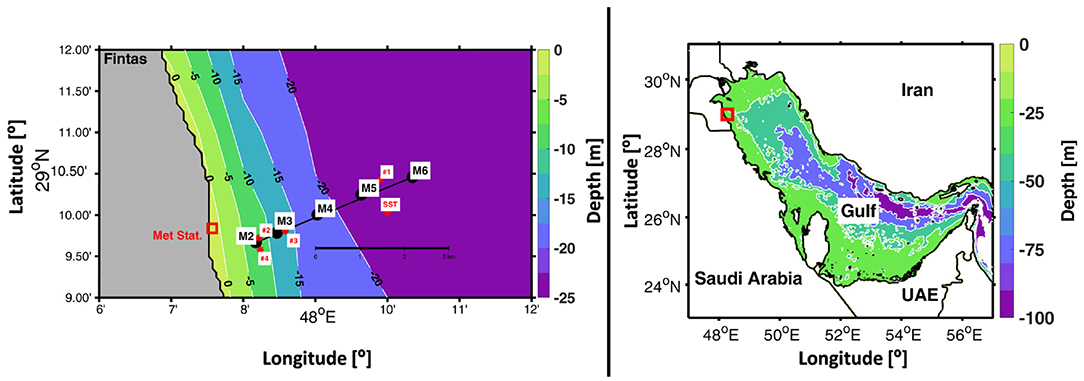
Figure 1. (Left) Schematic of the experimental setup off Fintas, Kuwait. Black circles represent locations of instrument moorings (M2-M6). Red circles represent the four locations (#1-4) where profiles of turbulence parameters and water-quality properties were collected as well as the sea surface temperature (SST) float. The location of the meteorological station is marked with a red box. (Right) Depth contours of the Gulf with the study location marked in red square.

Two observational approaches were used to obtain spatial and temporal data and derive the structure of the IWs: time series measurements and cross-shelf profiling. We obtained estimates of physical and turbulence parameters by applying the computation methods described below.

(1) Time series measurements: Five moorings (M2 to M6; Figure 1) were deployed along the sloping incline perpendicular to the coastline to capture IWs at various stages of disintegration and to track IW features over time and space. The orientation of the mooring array was designed to be in the expected main propagation direction of shoreward-moving IWs, i.e., along a line perpendicular to the coastline. To adapt the mooring array for optimal measurement of the disintegrating IWs, the five moorings were deployed in an arrangement that used exponentially increasing spacing between moorings (Figure 1). The exponential spacing of the moorings was designed to improve horizontal spatial resolution upon approaching the coastline where we expected much of the dissipation to occur due to the increase in the slope angle. The shallowing bathymetry in this region has a slope that increases roughly as an exponential function of the distance from the coastline. We note that eventually small adjustments were made during moorings deployment based upon the vessels' depth sounder. The spacing between moorings changed from 1,150 m (at a nominal water depth of 12 m) to 5,050 m (at a nominal water depth of 25 m) from the coast to the open sea off Fintas. Moorings were instrumented with bottom-mounted upward-looking Acoustic Doppler Current Profilers (ADCPs), Conductivity-Temperature-Depth loggers (CTDs) and temperature loggers positioned at various depths between the sea surface and seabed (Table 1).

TABLE 1

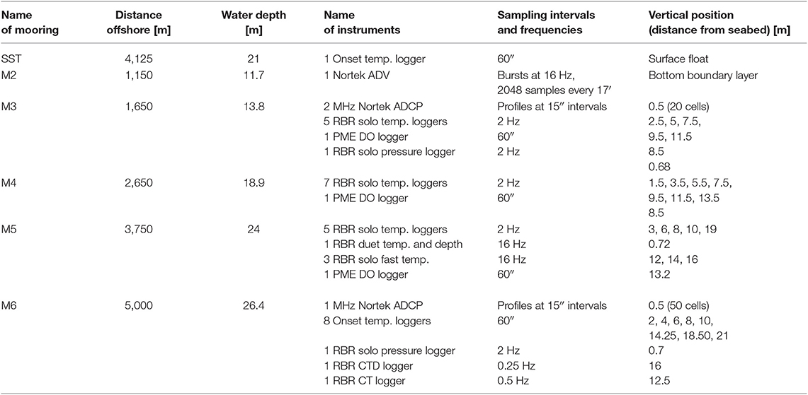
Table 1. Mooring and instrument details.

Furthermore, a bottom mounted Acoustic Doppler Velocimeter (ADV) at M2 (nominal water depth of 11.7 m) sampled 3 beam velocities and pressure at 16 Hz in bursts of 2,048 samples (duration of 128 s with 17 min intervals between bursts). Velocity data with signal-to-noise-ratios (SNR) >10 dB and correlation values >70% (Rusello, 2009) were despiked (Islam and Zhu, 2013). A total of 1001 (95%), out of 1,052 recorded bursts, passed quality control and were used for further analysis and estimates of TKE dissipation rates, ϵ.

The classical Kolmogorov –5/3 law allows estimation of ϵ, from the velocity wavenumber spectra in the inertial subrange

$\begin{array}{ll}{F}_{ii}(k)={\alpha }_i{ϵ}^{2/3}{k}^{-5/3},& (1)\end{array}$

where F_ii(k) is the velocity wavenumber spectrum, k is the wavenumber in the longitudinal (streamwise) direction, i represents the direction of velocity fluctuations (i = 1 is the longitudinal (streamwise) direction, i = 2 is the transverse (spanwise) direction, and i = 3 is the vertical direction), and α_i is a constant (Saddoughi and Veeravalli, 1994). In this study we used the vertical velocity (i = 3) for power spectrum density (PSD) estimates. Due to the ADV's beam configuration the vertical velocity exhibits a noise level lower by a factor of ~10 compared to the horizontal components (Voulgaris and Trowbridge, 1998; Khorsandi et al., 2012). For isotropic turbulence, α₃ = 0.65 (Pope, 2000).

Due to possible contamination of the velocity spectra by surface waves ϵ was estimated using a modified Kolmogorov –5/3 formulation proposed by Trowbridge and Elgar (2001):

$\begin{array}{ll}{S}_{ii}(f)=\frac{12}{55}\alpha U^{2/3}{ϵ}^{2/3}{f}^{-5/3}I(\frac{\sigma }{U},\theta ),& (2)\end{array}$

where I is a function of σ, the standard deviation of the horizontal velocities, U, θ is the angle between the current and waves, and α = 1.5 is the one-dimensional Kolmogorov constant (Saddoughi and Veeravalli, 1994). This modified method has previously been shown to be effective when applied to ADV measurements in the study of IW energy transport by Moum et al. (2007).

Using the 1001 bursts that passed SNR and Correlation quality control criteria, ϵ was computed using a linear fit in log-space to the one-dimensional velocity frequency spectrum. An estimate of ϵ was rejected when the fitted slope was outside an interval of −2.27 and −1.07. This criteria has been accepted and used by previous studies e.g., Sato et al. (2014) who measured IW's and turbulence in Patricia Bay, Canada. Using this approach, a total of 994 out of the 1,001 bursts (94%) were deemed to be suitable to estimate ϵ. An example of a burst that passes the quality control and fitting criteria is presented in Figure 2.

FIGURE 2

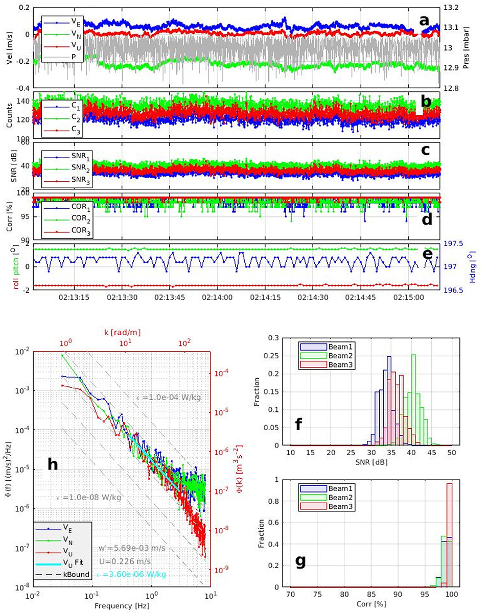
Figure 2. ADV burst example, 15 July, 2017, mooring M2. (a) Traces of east-west (blue), north-south (green), and vertical (red) velocity components, and of pressure (gray) as a function of time (the entire burst spans 128 s); (b) counts (signal strength) for each beam; (c) SNR for each beam; (d) correlations for each beam; (e) roll (red), pitch (green), and heading (blue) (allows detection of possible motion of the bottom pod); (f) histogram of SNR for each beam; (g) histogram of correlations for each beam; (h) PSD of the east-west (blue), north-south (green), and vertical (red) velocity components. Sloping broken gray lines represent values of ϵ from 10⁻⁸ to 10⁻⁴ W/kg. The solid cyan line represents a fit to the PSD of vertical velocity fluctuations.

Four moorings (M3–M6) were equipped with RBR conductivity-temperature (CT) loggers, Onset light sensors, Onset temperature sensors, and PME dissolved oxygen (DO) loggers equipped with wipers to help prevent marine fouling (see Table 1 for details). Additionally, the moorings included 17 fast-response RBR Solo temperature sensors recording at 2 Hz and three recording at 16 Hz. Each of the 20 fast-response temperature sensors was mounted on a winged frame which oriented the sensors into the flow to minimize possible flow disturbances from the mooring line and instrument wake. Another fast-response temperature-pressure sensor recording at 16 Hz was attached to the bottom pod at M5, pointing upward. Spectral estimates of temperature fluctuations measured by the moored sensors provided details on the spatiotemporal evolution of mixing activity in the water column (details in section 3.2.4).

Our interest in this study are the energetic tidally forced IW's which, based on spectral analysis (details in section 3.2.2), are limited to a period of 3 h (M₈ tidal harmonic). Thus, prior to further analysis, the ADCP velocity and temperature profiles were filtered using a second-order Butterworth low-pass filter to eliminate processes with time scales less than 2 h but retain low tidal modes (e.g., M₈ − O₁ tidal harmonics). Furthermore, the time series of profiles of the vertical velocity component, w, measured by the ADCP were used to provide a direct estimate of the IW kinetic energy (KE),

$\begin{array}{ll}KE=\frac{1}{2}\overline{w^2}.& (3)\end{array}$

As shown in Richards et al. (2013), using the vertical velocity component effectively isolates the large horizontal background processes and magnifies the vertical processes generated by IWs.

As part of the experiment, we deployed a full suite of meteorological sensors on a mast mounted at the pier of Kuwait University's Marine Science Center in Fintas (800 m from M2; Figure 1). The station provided measurements of surface meteorological parameters (air temperature and humidity, wind speed and direction, incoming shortwave and longwave radiation, and barometric pressure) at 1 min intervals to complement the oceanographic measurements. Net heat flux, $J_q^o$, and wind stress, τ, were computed from the meteorological measurements following the Coupled Ocean Atmosphere Response Experiment (COARE ver 3.5) formulation (Fairall et al., 1996, 2003). From τ and $J_q^o$ we computed the Monin Obukhov length scale, L, to predict when turbulence might be dominated by wind stress (L > 0) or by convective buoyancy loss at the surface (L ≤ 0),

$\begin{array}{ll}L=\frac{-u_{*}^3}{\kappa J_b^o},& (4)\end{array}$

where $u_{*}=\sqrt{\tau /\rho }$ is the friction velocity related to wind stress and density, κ = 0.4 is von Karman's constant, and $J_b^o$ is the surface buoyancy flux (Monin and Obukhov, 1954; Anis, 2006).

(2) Cross-shelf profiling: Free-fall turbulence profiling were carried out with Rockland Scientific's microCTD (512 Hz sampling rate) turbulence profiler that allows measurement of small-scale (order 1 mm) fluctuations of conductivity, temperature, and current shear from which ϵ was estimated. The free-fall (~0.7 m/s) profiler, took measurements during the descent. At the end of each profile, after the profiler landed on the seabed, it was pulled back to the surface by it's tether line ready to start the next profile. Profiles were taken continuously over the 5-day period—except short breaks to change watch teams—to provide adequate statistics of turbulence parameters throughout the water column. A total of 1,451 profiles were recorded over a 5-day period (15 to 20 July 2017) at the mooring sites (Figure 1; red circles).

Spectra were computed from current-shear measurements of two perpendicularly oriented sensors after being high-pass filtered using a first-order Butterworth filter. The resulting two shear datasets from both sensors were then grouped into 26 overlapping segments each with a vertical bin size of 1.4 m starting from ~1.75 m depth when the profiler reached it's nominal fall speed. Each segment included 1,024 samples (2 s bins) with 512 sample (50%) overlap. Each segment was windowed with a generalized Cosine window, and the fast Fourier transform (FFT) calculated.

$\begin{array}{ll}ϵ=\frac{15}{2}\nu \overline{{(\frac{\partial u}{\partial z})}^2}=\frac{15}{2}\nu {\displaystyle {\int }_0^{\infty }}\Phi (k)dk,& (5)\end{array}$

where ν is the kinematic viscosity, $\frac{\partial u}{\partial z}$ is the vertical shear of the horizontal velocity and Φ(k) is the shear spectrum. Noise was removed from the spectra which were then fitted with the empirical Nasmyth spectrum (Nasmyth, 1970; Osborn and Crawford, 1980; Oakey, 1982; Monin and Ozmidov, 1985; Bluteau et al., 2016) from which ϵ was estimated by integrating the fitted spectrum. A total of 1,218 out of the 1,451 profiles (84%) included estimates of ϵ for all segments.

An example of a spectrum of a single segment from the two shear probes and the fitted Nasymth spectra are presented in the top panel of Figure 3. The data was collected between 13.2 and 14.6 m depths (segment 16) at location #1 at midnight on 16 July, 2017. The increase in spectra for wavenumbers larger than 107 cpm (thin blue and red lines) is due to instrument noise and possible instrument vibration not detected by the accelerometer and was “cleaned” using Goodman's coherent noise reduction algorithm (thick red and blue lines) (Goodman et al., 2006). To minimize overestimation of ϵ due to noise, the Nasmyth spectrum was fitted to the observed shear spectrum (black lines) and integrated over a finite range. The finite range was set between 0 and the wavenumber of the spectral minimum (k_max) that is detected using a low-order polynomial fit (triangles). Using this approach resulted in ϵ values of 2.9 and 3.7 x 10⁻⁷ W/kg for the two shear probes. A total of 26 segments was used for each shear probe to construct the ϵ profiles (Figure 3; bottom panel). ϵ profiles from both shear probes were found to be in good agreement and for statistical robustness were averaged before further analysis.

FIGURE 3

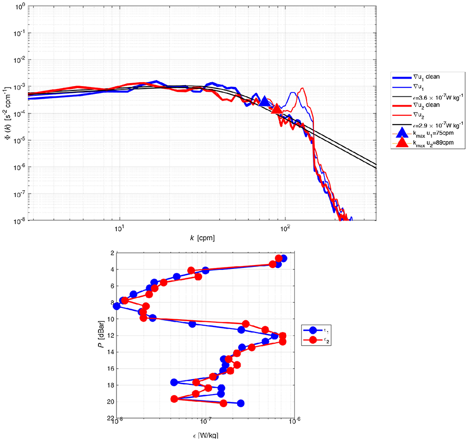
Figure 3. (Top) Example of spectra from the two shear probes, 1 (blue) and 2 (red), of the MicroCTD and the fit to the Nasmyth empirical spectra, July 16. 2017. Spectra before (thin lines) and after (thick lines) noise removal are shown as well. The curved black lines represent the Nasmyth spectra for ϵ₁ = 2.9 and ϵ₂ 3.7 x 10⁻⁷ W/kg. (Bottom) ϵ profiles comprised of 26 segments from the two shear probes taken at location #1.

The profiler was also equipped with a fluorometer and turbidity probe that provided chlorophyll a concentrations and turbidity profiles. Temperature and conductivity from the profiles was used to compute the density for estimates of the buoyancy frequency, N² (a measure of stratification), and the Richardson number, Ri, the ratio between N² and vertical shear, S². Ri has a theoretical threshold of Ri_c ≤ 0.25 for instability, but may range between 0.2 and 1.0, for unstable flows (Galperin et al., 2007), and was used here to quantify water column stability/instability conditions.

3. Results and Discussion

Next we present results of observations from the meteorological station (section 3.1), the five cross-shore mooring stations M2 to M6 (section 3.2), and two locations between the mooring sites where continuous turbulence profiling was conducted (section 3.3) (Figure 1).

3.1. Meteorological Conditions

During the 12-day study period, we recorded both continental northwesterly winds and maritime southeasterly winds (directions indicate where the wind is blowing from). The continental northwesterly winds (Figure 4A; red shading) produced drier and hotter conditions with an average relative humidity of 19% (Figure 4D) and a maximum air temperature of 49.1°C, on the afternoon of 17 July (Figure 4C). This maximum temperature measurement is classified as extremely hot (99th percentile) for the month of July according to a 42-year (1958—2000) study of extreme temperature events in Kuwait by Nasrallah et al. (2004). The largest measured diurnal temperature range of 11.1°C also occurred during the period of northwesterly winds on 17 July.

FIGURE 4

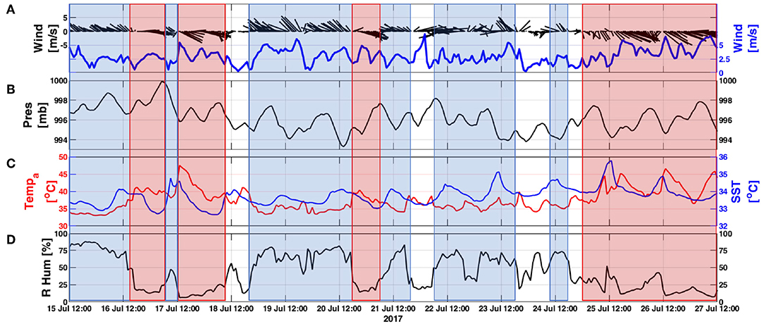
Figure 4. Hourly averages of meteorological measurements from the station located on the coastal pier in Fintas. (A) wind velocity vectors (black) and speed (blue); (B) barometric pressure; (C) air temperature (red) and SST (blue); (D) relative humidity. The blue and red boxes overlaid on each graph represent the southeasterly and northwesterly wind periods, respectively. Time is UTC.

In contrast, the maritime southeasterly winds (Figure 4A; blue shading) produced up to 90% relative humidity and cooler conditions, with air temperature ranging from 33 to 40°C. These winds produced diurnal air temperature ranges as large as 8.6°C, smaller compared to those during the northwesterly winds. The diurnal air temperature changes throughout the study period caused the sea surface temperature (SST) to follow a well-defined diurnal pattern that varied from 0.6 to 2.7°C (Figure 4C).

Despite differences between northwesterly and southeasterly winds in producing abrupt changes in humidity and air temperature in periods as short as 25-min, wind speeds were moderate with hourly averages of 3.7 m/s (maximum 8.1 m/s) and 2.9 m/s (maximum 6.1 m/s), respectively.

3.2. Cross-Shore Mooring Observations

3.2.1. Horizontal Currents Background

The tides in the study region were dominated by a semidiurnal tide with elevations ranging from 0.57 m (mid-neap, 18 July) to 2.91 m (mid-spring, 25 July). This range was consistent across the cross-shore moorings within 0.05 m.

The horizontal current profiles at both ends of the study region (M6 and M3) followed a similar direction but differed in their magnitude. The maximum recorded current speed at M6 was 0.78 m/s, while that at M3 was 0.68 m/s. These maximum current speeds were obtained at mid-depth (between 56 and 65% of the water-column depth), during mid-ebb (3.4 h after HW), and during mid-spring (afternoon 25 July). Similarly, the north-south (N-S) and east-west (E-W) currents were observed to consistently follow the tidal phase, with maximum current velocities of 0.49 m/s (E-W) and 0.59 m/s (N-S) observed at mid-spring.

3.2.2. Vertical Currents and IW Energy

Understanding the dynamics of vertical motions and their variability is crucial for the detection and analysis of IWs. To this end, we focused on the vertical velocity profiles and the KE associated with them as a proxy for wave energy (Equation 7), at both ends of the cross-shore moorings (M6 and M3). The vertical currents at M6 showed a net upward velocity during LW (max 4.2 mm/s on 25 July) and a net downward velocity during HW (max 7.8 mm/s on 23 July). In contrast, at M3 a net upward velocity was observed during tidal flooding and downward velocity during ebbing, which may suggest that the IW signal maybe a product of tidal constituents.

To this end, we estimated vertical velocity spectra from the 15 min ADCPs profiles at both M6 and M3 between 15 and 27 July and compared the vertical velocity oscillation periods with those of the tidal oscillation periods associated with changes in sea surface elevation. This is presented in Figure 5, where elevated pressure spectral levels (green) are associated with possible tidal constituents marked at the top of the figure. The semidiurnal (M₂ and S₂) and diurnal (O₁ and K₁) tidal constituents accounted for 95% of the total tidal kinetic and potential energy. The vertical velocity spectral levels at both M6 (light blue) and M3 (dark blue) associated with these four major tidal constituents were more than twice as large as those of the other constituents. This suggests that IW in the northern Gulf are likely to be a result of the interaction of the O₁, K₁, M₂, and S₂ constituents as they propagate into the region.

FIGURE 5

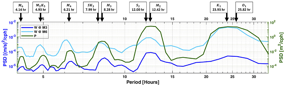
Figure 5. PSD of vertical velocities at M6 (light blue) and M3 (dark blue), computed as the average of all vertical cells, and pressure (green) from 15 to 27 July, 2017. Black arrows indicate tidal constituents during periods when pressure spectral levels appear elevated.

The 12-day time series of wave KE at M6 and M3, shown in Figure 6B2, was computed from the observed vertical velocities. The wave energy at M6 closely followed the changes in the tidal phase (Figure 6A), with energy ranging from 8 × 10⁻⁸ (mid-neap; 16 July) to 8 × 10⁻⁵ (mid-spring; 25 July) m²/s², indicating more energetic waves during spring phase (Figure 6B1). A similar effect was seen at M3, where the energy ranged from 1 x 10⁻⁸ (neap) to 4 × 10⁻⁶ m²/s² (spring), suggesting that the wave energy in deep water exceeds the energy in shallower water.

FIGURE 6

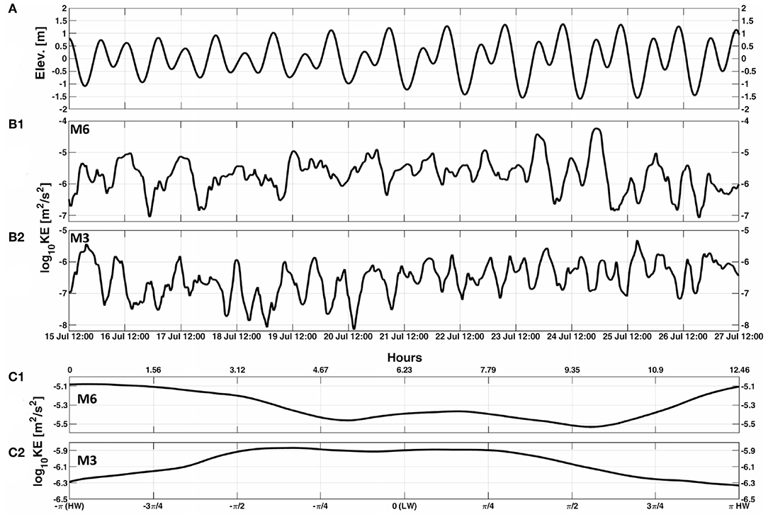
Figure 6. Wave energy at moorings M3 and M6 recorded from 15 to 27 July, 2017. (A) sea surface height variability; (B) KE computed from vertical velocity observations at M6 (B1) and M3 (B2); (C) phase averaged KE at M6 (C1) and M3 (C2). Time in the upper axis of subplot C indicates hours into the M₂ surface tide.

To further emphasize the relation between the tidal phase and IW energy, we computed the phase average of KE (Figure 6C). The phase and depth averaged KE in Figure 6C1 clearly show that IW energy oscillates in sync with the tidal phase and that the IW energy is approximately twice as large during HW than LW at M6 (Figure 6C1). This appears to be consistent with study results by Richards et al. (2013), who reported the IW energy to be twice as high during HW than during LW at depths similar to this study (~23 m). However, in contrast to both results, a clear phase lag was observed at M3, and during HW the energy was 65% of that observed during LW (Figure 6C2). To compute the phase lag, we compared the time at which the KE peaked (on wave arrival) at M3 and M6. At M6, KE peaked at a tidal phase of 1.1 h, while at M3, KE peaked at 4.2 h, suggesting a lag of 3.1 h. The 3.1 h phase lag, and a distance of 3350 m between M6 and M3, suggests an IW propagation speed of 0.30 m/s for the 12-day period. It appears from the above results that once these IWs are generated, they start to drift out of the surface tide phase as they propagate landward. These observations are consistent with those demonstrated by Shroyer et al. (2011),Ponte and Klein (2015), and Buijsman et al. (2017) for tidally forced IWs on continental shelves of the global oceans.

3.2.3. Thermal Structure

The lowest measured water temperature during the 12-day study period was 32.19°C at M6 near the seabed in the afternoon of 15 July, 2017. Correspondingly, the air temperature on 15 July was the coolest (33°C) during the study period, which may explain the relatively low water temperatures on that day. When air temperature and SST were at a minimum, the change of temperature with depth was the largest at all locations, with a maximum surface to bottom difference of −1.33°C recorded at M3 and a minimum difference of −0.99°C recorded at M6. The highest water temperature (34.57°C) was recorded at M3 near the sea surface in the afternoon of 25 July. Overall, the daily average water temperature increased over the study period. The largest increase (1.26°C, from 31.47 to 32.73°C) was observed at M3, and the smallest at M6 (1.02°C, from 32.72 to 33.74°C).

3.2.4. Thermal Structure and IWs Activity

Visual examination of the thermal structure at M6 to M3 (Figure 7) reveals IW activity with significant semidiurnal oscillations in the thermocline between 15 to 17 July (neap) and 23 to 25 July (spring) (thermocline depth is defined here as the depth where the largest vertical gradient of temperature was observed). This suggests that IWs occur chiefly during neap and spring tides and is different than reported in other studies where IW activity is often absent during neap tides (e.g., Apel, 2002). In contrast, a study by Shroyer et al. (2011) on the New Jersey continental shelf showed that tidally forced IWs during neaps are ten times more energetic with twice the amplitude than during springs. This unpredictable nature of IWs is due to their susceptible to refraction at a given location due to the time varying background low frequency circulation, stratification gradients, relative vorticity all which may force it out of the surface tide phase (Buijsman et al., 2017).

FIGURE 7

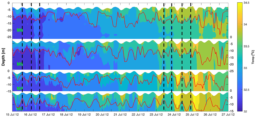
Figure 7. Two hour low-pass filtered thermal structure at the four mooring stations M6 to M3 (top to bottom panels) from 15 to 27 July, 2017. The horizontal red solid line represents the thermocline depth and the vertical black dashed lines indicate periods of HW with noticeable IW activity. Time is UTC.

Despite the relatively low KE at M3 compared to that at M6 (Figures 6C1,C2), the undulation seen during the two noticeable periods (15 to 17 and 23 to 25 July) of IW activity reveals larger amplitudes (computed as the changes in thermocline depth) of about 9 m in the shallower waters at M3 compared to about 6 m in the deeper waters at M6 (Figure 7). Furthermore, the apparent thermocline oscillation appears to be out of phase at M6 and M5 when compared to that at M4 and M3. This observation is consistent with the phase lag observed in the vertical current velocities and KE between M6 and M3, and may explain the phase lag observed in the thermocline oscillation pattern.

To further analyze the thermal conditions in the thermocline, we focused on the temperature time series measured by the fast-response temperature loggers located in the thermocline at locations M5 and M3 (Figures 8A,B). These stations were selected because they were the nearest (M3) and the farthest (M5) from the shore where fast temperature loggers were available during the two periods of noticeable IW activity.

FIGURE 8

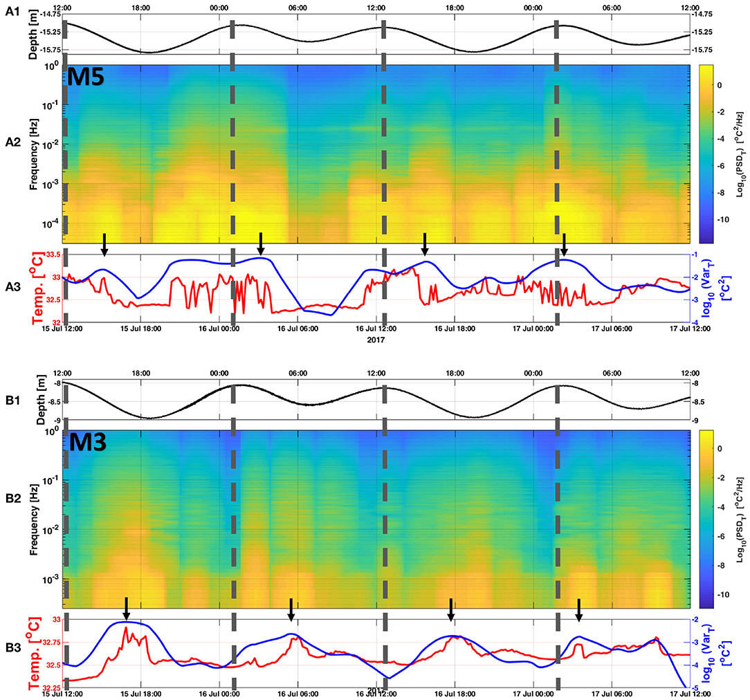
Figure 8. (A1) Temperature logger depth at M5. (A2) Spectrogram obtained from temperature time series measured by a fast-response temperature logger located at the thermocline during 2 days of IW activity at M5. (A3) 10 min averaged temperature trace (red line) and temperature variance (log10 scale; blue line). (B1–B3) are similar to (A1–A3) but for M3. Vertical dashed lines indicate periods of HW, and black arrows indicate periods of maximum temperature variance during each of the four tidal cycles. Time is UTC.

At M5, where fast temperature loggers (16 Hz sampling rate) were deployed, temperature spectrograms and variances were computed in blocks of 65,536 samples (~68 min; Figure 8A2). Both the spectral and variance levels at mid-depth (~15 m) roughly follow a semidiurnal cycle. Larger temperature fluctuations during these cycles are clearly observable in the temperature trace as well as in the variances (Figure 8A3). These semidiurnal bursts of elevated spectral and variance levels at mid-depth follow the vertical oscillation of the thermocline associated with the IW activity. To track the temperature variance changes with depth associated with the oscillation of the thermocline we computed the temperature variances at M5 using eight fast response temperature loggers, in a similar approach as above. Results of this approach are shown in Figure 9, where the depth at which the maximum temperature variance appears (indicated by the horizontal black line) to correlate well with the thermocline oscillation (indicated by the horizontal red line). During the surface tidal flooding phase, the thermocline progressed downward and closer to the temperature loggers located at mid-depth, resulting in elevated spectral and variance levels (Figures 8A, 9). In contrast, during the surface tidal ebbing phase, the thermocline progressed upwards and further away from the temperature loggers located at mid-depth, resulting in lower spectral and variance levels.

FIGURE 9

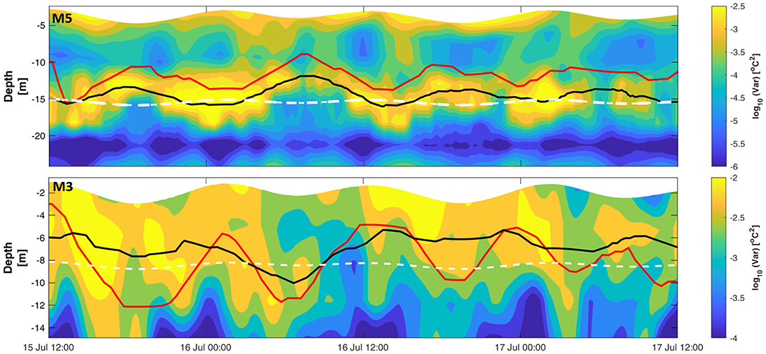
Figure 9. Temperature variance (log10 scale) computed from the temperature loggers at M5 (Top) and M3 (Bottom). Horizontal black and red lines indicate the depths of maximum temperature variance and thermocline, respectively. The white dashed lines indicate the depth of the temperature logger in Figure 8. Time is UTC.

Compared to mooring M5, the spectral levels at M3 (sampling rate of 2 Hz, blocks of 8,192 samples, ~68 min) were lower during HW (Figures 8B2,B3) but were consistent with M5 by roughly following the semidiurnal cycle. The maximum temperature variance for the four tidal cycles at both locations (indicated by black arrows in Figures 8A3,B3) had a time lag of 1.8 h between M5 and M3 during the first three tidal cycles. Using the distance of 2,100 m between M5 and M3 this time lag yields an IW speed of 0.31 m/s between 15 and 17 July, similar to that computed from the phase lag of the KE between M6 and M3.

3.3. MicroCTD Observations

3.3.1. Location #1 (15–16 July)

The first day of turbulence profiling was conducted 550! m east of M5 and 741 m west of M6 (Figure 1) between the afternoons of 15 and 16 July. Winds during the first 5 h of this period were fair southeasterlies with maximum speeds of 5.7 m/s. By the end of the profiling period, winds weakened to less than 3.5 m/s (Figure 4A).

Examination of the thermal structure revealed a general diurnal heating of the upper water column (0–7 m) (Figure 10C). Peak daytime solar radiation was 909 W/m² with a maximum net surface heat flux of 582 W/m² (Figure 10B). Daytime heating was confined to the upper ~7 m layer, i.e., above the thermocline, and resulted in lower than the nighttime water density of 1,026 kg/m³ (Figure 10E). Visual inspection of the thermocline (Figure 10C), halocline (Figure 10D), and pycnocline layers (Figure 10E) reveals a clear semidiurnal pattern with the layers being located deeper (~14.7 m) during HW than during LW (~7.1 m). This is further emphasized in the one day waterfall plot in Figure 11, where the density profiles clearly show a two layer system divided by a pycnocline(albeit relatively weak) which oscillates in-phase with the tide. It is worth noting that the vertical advection of chlorophyll a, being in sync with the vertical movement of the pycnocline, forced the depth of maximum chlorophyll a concentration to decrease during LW and increase during HW (Figure 10C; yellow dots). The advection of chlorophyll a to upper water layers during LW may have contributed to the lower mid-depth DO concentrations (not shown), similar to results reported previously by Wang et al. (2007). The effect of vertical advection is further emphasized by the vertical transport of turbid waters near the bed upward from 14 to 8 m depth during the ebbing phase and downward from 8 to 14 m depth during the flooding phase (Figure 10D).

FIGURE 10

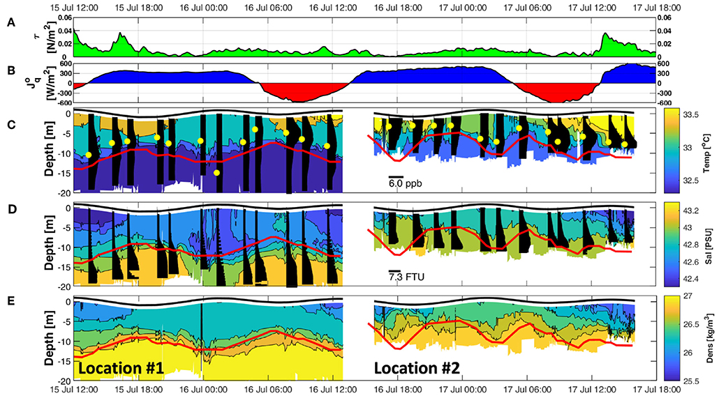
Figure 10. Meteorological and microCTD's hydrography measurements at locations #1 and #2. (A) wind stress; (B) net heat flux where negative (red shading) and positive (blue shading) values indicate net heating or cooling, respectively; (C) temperature contours (color) and chlorophyll a concentrations (black bars with maximas indicated by yellow dots; PPB); (D) salinity contours (color) and turbidity (black bars; FTU); (E) density contours (color). Solid red lines in (C–E) indicate the thermocline depth estimated using the temperature loggers at M3 and M6. Time is UTC.

FIGURE 11

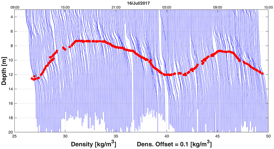
Figure 11. Waterfall plot of density computed from the microCTD profiles at location #1. The red circles mark the pycnocline depth.

Stability in the upper layer was primarily influenced by surface forcings (τ and $J_q^o$) and IW activity. Daytime heating in the upper layer yielded higher buoyancy frequencies than during nighttime (Figure 12B). However, the enhanced buoyancy frequency in the upper layer on the afternoon of 15 July appeared insufficient to maintain a stable upper layer (Ri > 0.25; Figure 12C) in contrast to the following afternoon of 16 July. This was likely a result of the higher wind stress on the afternoon of 15 July (up to 0.05 N/m²; Figure 10A) generating increased vertical shear levels in the upper layer (Figure 12A) and reducing Ri values (Ri < 0.25; Figure 12C), leading to unstable conditions. The instability in the upper layer during the afternoon of 15 July corresponds to higher turbulence levels, as indicated by the larger values of ϵ (~10⁻⁵ W/kg). Between early morning (4:30) and afternoon of 16 July, lower values of ϵ (~10⁻⁸ W/kg) were observed (Figure 12D).

FIGURE 12

Figure 12. MicroCTD measurements at locations #1 and #2. (A) microstructure shear; (B) buoyancy frequency; (C) Ri number (gray shading; Ri < 0.25); (D) dissipation rate of the TKE. Solid red lines indicate the thermocline depth estimated using the temperature loggers at M3 and M6. Time is UTC.

The highest stability was observed in the thermocline region with buoyancy frequencies exceeding 10⁻⁴ 1/s², larger Ri (> 0.25), and reduced values of ϵ (Figures 12B–D). The layer beneath the thermocline, defined here loosely as the bottom boundary layer (BBL) was subject to bursts of enhanced shear instabilities (≥ 0.1 1/s²) occurring during both flood and ebb cycles, with the lowest values of shear (< 0.1 1/s²) observed during tidal slack. These shear instabilities resulted in lower Ri (Ri < 0.25) and ϵ values higher than 10⁻⁷ W/kg (Figures 12C,D). We note that shear during the two flood phases was ~30% lower than during the two ebb phases, and appears to be consistent with the increase in horizontal current speed during ebb. The role of tidally forced IW's in producing near bottom intensified shear, ϵ, and turbidity values compared to other parts of the water column has been reported also by other studies (e.g., Richards et al., 2013). The latter study analyzed semidiurnal internal tides at Ile aux Lievres island, Canada, observing ϵ values up to 10⁻⁴ W/kg and shear values up to 0.15 1/s² in the BBL during the ebbing phase, double the water column average.

In order to examine the generation of IWs at the diurnal and semi-diurnal frequencies, we next investigate the variation in the magnitude and vertical structure of these waves using vertical mode theory (Phillips, 1977; Gill, 1982). Assuming a flat seabed, the vertical structure of these modes can be derived using the buoyancy frequency computed from the microCTD density profiles collected at location #1,

$\begin{array}{ll}\frac{\partial }{\partial z}\left(\frac{1}{N^2-{\omega }^2}\frac{\partial {\psi }_i}{\partial z}\right)+\frac{1}{c_i^2}{\psi }_i=0.& (6)\end{array}$

This approach determines the eigen speed, c_i, and the vertical isopycnal displacement ψ_i, of the ith (i = 1–3) mode assuming homogeneous boundary conditions such that ψ(0) = ψ(H) = 0, where H is the water depth (Kelly et al., 2013). The modes were computed using the IWs frequency, ω, of both semi-diurnal (S₂ 12 and M₂ 12.42 h) tides and both diurnal (K₁ 23.93 and O₁ 25.82 h) tidal periods. Using this approach and the dispersion relation, the theoretical group, c_g, and phase speeds, c_p, were for the four tidal frequencies computed

$\begin{array}{ll}{c}_g=\frac{{({\omega }^2-f_c^2)}^{1/2}}{\omega }{c}_i,& (7)\end{array}$

$\begin{array}{ll}{c}_p=\frac{\omega }{{({\omega }^2-f_c^2)}^{1/2}}{c}_i.& (8)\end{array}$

where f_c is the Coriolis frequency at our mooring's latitude 29°10′ (Rainville and Pinkel, 2006).

This method is widely used to analyze the variations in dynamical modes associated with IW propagation e.g., MacKinnon and Gregg (2003) on the New England Shelf, Ross et al. (2014) in the Fjords of Chile, Stephenson et al. (2015) on the Celtic Sea Shelf, and by Zhang et al. (2016) on the Iberian Continental Margin. Results of the vertical structure of modes 1–3 are presented in Figure 13. The largest values of the buoyancy frequency were found at the pycnocline depth (9 m) (Figure 13A). The vertical displacement, based on the depth and stratification conditions observed at location #1, indicate that both diurnal and semi-diurnal (solid black; Figures 13B,C) closely responded to the first mode than to the second mode. The vertical displacement structures for mode-3 were close to zero. Mode-1 for both semi-diurnal and diurnal IWs peaked at the pycnocline depth, while mode-2 peaked at depths 6 and 13 m. Moreover, both modes-1 and 2 vertical displacement during semi-diurnal IWs were about twice in magnitude compared to those of the diurnal IWs. Thus, the existence of the diurnal and semi-diurnal IWs described using the above approach appears to be consistent with the previous results described in section 3.2.2. In addition, the theoretical semi diurnal (S₂ and M₂) mode-1 IW average phase and group speeds were 0.46 and 0.36 m/s, respectively. While the diurnal K₁ mode-1 IW average phase and group speeds were 3.31 and 0.09 m/s. However, both theoretical phase and group speeds for the O₁ tidal constituents were near infinity and zero, respectively, ruling out the possibility of O₁ frequency IW's despite the elevated pressure and vertical velocity spectral levels observed in Figure 5. Further analysis of these elevated spectral levels at the O₁ frequency will be presented in future work.

FIGURE 13

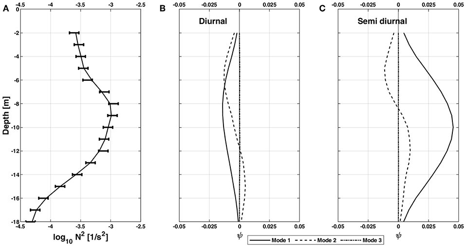
Figure 13. (A) Buoyancy frequency squared profile averaged over location #1 profiling period; and the normalized vertical displacement mode structures (modes 1 to 3) for the (B) diurnal K1 tide frequency and (C) semi-diurnal (averaged between S₂ and M₂ tides) tide frequency.

3.3.2. Location #2 (16 – 17 July)

The second day of profiling was conducted 122 m east of M2 and 410 m west of M3 (Figure 1) from 16:00 on 16 July to 17:00 on 17 July. Wind stress during this period was low (< 0.01 N/m²) until the last 3 h when northwesterly winds strengthened to a speed of 5.9 m/s, doubling the wind stress to 0.02 N/m² (Figure 10A). As described in section 3.1, the maximum air temperature was 49.1°C with a maximum drop in day-to-night temperature of 11.1°C. Furthermore, during this period, the humidity was about half that during the previous day (Figure 10D), resulting in surface heat flux loss larger by ~30% compared to the previous night (Figure 10B). Similar to location #1, daytime heating caused the layer above the thermocline to warm by an average 0.6°C (Figure 10C) and its buoyancy frequency to triple (Figure 12B).

Unlike location #1, the combination of large day-to-night temperature drop, low humidity, and high net surface cooling produced by the northwesterly winds at location #2 induced favorable free convection conditions. This is indicated by near-zero Monin-Obukhov length scales and higher buoyancy losses of up to 2.5 × 10⁻⁷ W/kg, i.e., more than double the maximum observed during profiling at location #1 (Figures 14A,B).

FIGURE 14

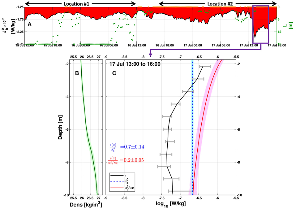
Figure 14. Surface buoyancy flux and MicroCTD measurements at location #2. (A) Surface buoyancy flux loss in red shading; dots represent the Monin Obukhov length scale to show when turbulence might be dominated by wind stress (green; L > 0) or by convective buoyancy loss at the surface (orange; L < 0). The blue and magenta boxes represent 3 h periods of pre and during possible convective conditions, respectively; (B) 3 h averaged density profile (green line) with their 95% confidence intervals in shading; (C) 3 h averaged profiles with their 95% confidence intervals of ϵ (black line), and production terms of TKE by wind (red line; $u_{*}^3/\kappa z$) and buoyancy (blue line; $J_b^o$). Time is UTC.

To further examine these convection conditions, we focus on the 3 h of high surface buoyancy losses of >2 × 10⁻⁷ W/kg that occurred between 13:00 and 16:00 17 July. These high buoyancy losses coincided with increase in wind speed, maximum recorded air temperature and SST drop (Figure 4) likely responsible for the convective conditions (Figure 14A). The layer between the surface and thermocline was unstable (Ri < 0.25; Figure 12C) during these hours leading to an average ϵ value of 1.2 × 10⁻⁷ W/kg, about an order of magnitude higher compared to the average value of 1.1 × 10⁻⁸ W/kg observed 3 h prior to this period. However, they were not as high as the ϵ values of 10⁻⁶ W/kg observed near the bottom between 3:00 and 5:00 17 July when the BBL current speed and shear intensity reached their maximal values (Figure 15).

FIGURE 15

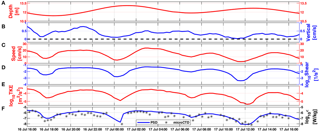
Figure 15. ADV data collected during microstructure profiling at location #2. (A) water depth; (B) vertical velocity; (C) horizontal current speed; (D) vertical shear of horizontal velocity computed with the assumption that the flow at the seabed is zero; (E) TKE (log10 scale) computed from the vertical velocity; (F) TKE Dissipation rate (log10 scale) estimated from the vertical velocity PSD (blue) and from the microCTD measurements within the BBL (black asterisks). Time is UTC.

To assess the role of surface buoyancy flux and wind stress to the TKE dissipation rate during these unstable, convective conditions, we examined their contribution to TKE production. This is similar to the idea behind the parameterization suggested first by Shay and Gregg (1986) and Lombardo and Gregg (1989). Here, in the upper layer, the ratio ($\frac{ϵ(z)}{J_b^o}$) was found to be 0.70, which is roughly double the second peak ratio of 0.42 observed at 6:00 17 July and higher compared to the period average of 0.16. This ratio is also consistent with those obtained by Anis and Moum (1992) for night convection in the open ocean, where it is in the range of 0.69 to 0.87 (Figure 14C). Our results are also similar to those of Shay and Gregg (1986) Bahama's experiment of 0.61 to 0.72, but are higher compared to Lombardo and Gregg (1989) observations of 0.45 to 0.65. The ratio for production of TKE by wind stress, ($\frac{ϵ(z)}{u_{*}^3/\kappa z}$), was found to be 0.20 (±0.05), despite an increase in wind stress from 0.01 to 0.04 N/m². These ratios indicate the clear role of convection in producing the observed instability and deepening of the mixed layer (Figure 12D).

Noticeable IW activity, observed between 15 and 17 July (section 3.2.4), resulted in the thermocline undulating in sync with the semidiurnal tidal phase (Figure 7) at both M3 and location #1. The thermocline following of the semidiurnal cycle at M3 was also consistent with the observed upward mean velocity during flood and downward during ebb. As expected from the results at M3 and location #1, the thermocline at location #2 followed the tidal cycle, moving downward during the ebb period and upward during flood between depths of 5 and 12 m. However, toward the last tidal cycle between 9:00 and 16:00 on 17 July, the thermocline deepened to undulate between 10 and 15 m depth (Figure 10C). This may be explained by the daytime heating on 17 July which produced the largest net heating of 617 W/m² (Figure 10B), commensurate with the highest recorded air temperature of 49.1°C and low humidity of <25%. The maximum buoyancy frequency (0.001 1/s²) and Ri values > 0.25 (Figures 12B,C) in the layer above the thermocline, observed between 9:00 to 12:00 17 July, may have in turn confined the thermocline to oscillate deeper, between 10 and 15 m depths. These surface stratified conditions suppressed mixing resulting in the lowest ϵ values (<10⁻⁹ W/kg) recorded during this study. Later, between 13:00 and 16:00 17 July, the upper layer deepened and stratification weakened (Ri < 0.25) due to convection, pushing the thermocline oscillation deeper.

As observed at location #1, the BBL was subjected to bursts of enhanced shear instabilities (≥ 0.1 1/s²) during both the flood and ebb cycles, with the smallest values (< 0.1 1/s²) occurring during slack periods (Figure 12A). Shear instabilities during both ebb and flood resulted in Ri values < 0.25 and ϵ values >10⁻⁷ W/kg (Figures 12C,D), similar to those observed at location #1. To further understand the BBL dynamics, we analyzed the ADV measurements at M2, which provided a detailed picture of the flow conditions ~1.1 m above the seabed and at a nominal depth of 11.7 m (Figure 15A). The results show that during slack periods, horizontal current speeds decreased to less than 0.1 m/s (Figure 15C), followed by a reduction in the vertical shear to less than 0.003 1/s² (Figure 15D), assuming zero flow at the seabed (Salon et al., 2008). During this tidal slack phase the values of TKE and ϵ reduced to < 3 x 10 ⁻⁵ m²/s² and < 10⁻⁷ W/kg, respectively (Figures 15E,F). During the weak turbulence conditions, upward vertical velocities decreased to values less than 0.2 cm/s (Figure 15B).

In contrast, during ebb and flood phases, horizontal currents were more than twice in magnitude than during tidal slack, with a maximum speed of 0.26 m/s. The higher vertical shear (> 0.01 1/s²) was consistent with the faster currents, and resulted in an increase in turbulence as indicated by the relatively high TKE and ϵ values of > 10 ⁻⁴ m²/s² and > 10⁻⁷ W/kg, respectively. The periods of maximum mixing observed by the ADV at 03:00 on 17 July were consistent with the elevated values of ϵ (10⁻⁶ W/kg) obtained from microCTD profiles at location #2 during the same time. During these elevated turbulence conditions, the mean upward vertical velocities increased to more than 0.5 cm/s (Figure 15B).

For the large Reynold numbers, Re = UL_n/ν, observed during this experiment (Re ~2 × 10⁶, where we used representative values of U = 0.2 m/s, L_n = 10 m, and ν = 10⁻⁶ m²/s) and assuming homogeneous and isotropic turbulence, we expect a well-separated region of wavenumbers lying between that of the energy containing eddies and the dissipative viscous scales (e.g., Tennekes and Lumley, 1972; Pope, 2000). This region is the inertial subrange in which the energy spectrum, F_ii(k), is predicted to follow the famous Kolmogorov minus five-thirds law (Equation 1) (Kolmogorov, 1968; Tennekes and Lumley, 1972; Monin and Ozmidov, 1985).

A cornerstone in dissipation scaling of turbulence is ϵ ≈ U³/l, where U and l are the velocity and integral length scales, respectively, which characterize the energy-containing turbulent eddies which inject the TKE (e.g., Vassilicos, 2015). To estimate the time scale (frequency) associated with the energy-containing turbulent eddies we estimated their representative velocity scale as ${\text{w}}^{*}\approx \sqrt{(var(w^{\prime }))}$, where w′ is the vertical velocity component measured by the-near bottom mounted ADV. The integral eddy length was assumed as the distance of the ADV's measurement volume above the bottom, i.e., 1.1 m. The resulting average time scale for the energy-containing turbulent eddies, t ≈ l/w′, is 41 s, with a max of 100 s. It is likely that energy-containing eddies in other parts of the water column may have larger integral and time scales.

To summarize—hydrography and microstructure measurements at locations #1 and #2 indicate that IW activity followed a semidiurnal cycle consistent with the observations of vertical velocities, KE (section 3.2.2), and thermal structure (section 3.2.4). Furthermore, similar to location #1, the maximum chlorophyll a concentration (Figure 10C) generally followed the thermocline vertical undulations spanning a vertical range of about 9 m.

4. Conclusions

This work offers the first detailed study of IW characteristics in the northwestern Gulf off the coast of Kuwait. These waves were detected through their induced changes in temperature, salinity, density, currents, turbidity, chlorophyll a, and the resulting turbulence. The vertical velocity data revealed that IW activity closely followed the semidiurnal and diurnal tidal cycles. This was further emphasized by the vertical velocity spectra which clearly indicated elevated spectral levels during four peak periods commensurate with the major tidal constituents O₁, M₂, and S₂. Our results appear to be consistent with other studies which indicate the role of semidiurnal tides (e.g., Bourgault and Kelley, 2003; Richards et al., 2013) and the role of multiple tidal constituents (e.g., Colosi et al., 2001; Sun and Pinkel, 2012) in the generation of IWs.

IWs, with amplitudes ranging from 7 to 9 m, were found to propagate toward the shore at an average speed of 0.31 m/s. Larger amplitude waves were observed closer to the shore. The changes in meteorological conditions associated with the northwesterly and southeasterly winds contributed to variability in the water column stability conditions. At times, IW activity was disrupted and forced to propagate deeper due to enhanced stratification in the surface layer resulting from extreme heating periods during exceptional hot and dry conditions. In addition, surface heat losses coinciding with increase in wind speed, drop in humidity, maximum recorded air temperature, and SST drop associated with the northwesterly winds led to convective conditions which led to instability and deepening of the mixed layer.

At the thermocline depth, the buoyancy frequency was higher and current shear was lower compared to the rest of the water column. This resulted in larger Ri values indicating suppression of mixing intensity in the thermocline. Highest TKE dissipation rates (> 10⁻⁷ W/kg) were observed to occur in bursts in the BBL, following the tidal cycle, and were closely tied to enhanced shear instabilities during both flood and ebb. Shear was lowest during tidal slack. We also note that shear instability during ebb was ~30% higher than during flood, resulting in more intense mixing beneath the IW's crest. These observations are in agreement with results of Richards et al. (2013) who observed a similar increase in BBL shear (water depth of 23 m) following the semidiurnal tidal cycle at Ile aux Lievres island, Canada, during summer.

Future work is planned to explore IW propagation in the far-field, before the IWs encounter the slope and start to breakup, to provide additional spatial and directional information on the undisturbed incoming waves. Further in-depth observational studies of wind-forced and thermally-driven convection in the Gulf should also provide new insights on formation of the GDW and its spilling into the Indian Ocean as well as a better understanding of the relation to the circulation in the Arabian sea. Lastly, the detailed physical oceanographic and surface meteorological datasets collected during this study should be useful for testing and improvement of present and future regional numerical circulation models, in particular due to the scarcity of such observations in the Gulf.

Data Availability Statement

The raw data supporting the conclusions of this article will be made available by the authors, without undue reservation, to any qualified researcher.

Author Contributions

FA and AA contributed equally in data collection, data analysis, and manuscript preparation.

Funding

This study was funded by the Kuwait Foundation for Advancement of Sciences (project #P21644SE01).

Conflict of Interest

The authors declare that the research was conducted in the absence of any commercial or financial relationships that could be construed as a potential conflict of interest.

Acknowledgments

We thank the Kuwaiti Coast Guard for providing field logistics, transportation and divers, and graduate students Mr. Sergey Molodtsov (Texas A&M University, USA) and Mr. Ahmed Al Rawahi (Sultan Qaboos University, Oman) for assistance in the field. We are also grateful to Mr. Evan Cervelli (Rockland Scientific) for providing technical assistance during the field campaign.

References

Al Senafi, F., and Anis, A. (2015). Shamals and climate variability in the Northern Arabian/Persian Gulf from 1973 to 2012. Int. J. Climatol. 35, 4509–4528. doi: 10.1002/joc.4302

CrossRef Full Text | Google Scholar

Alford, M. (2003). Redistribution of energy available for ocean mixing by long-range propagation of internal waves. Nature 423, 159–162. doi: 10.1038/nature01628

PubMed Abstract | CrossRef Full Text | Google Scholar

Anis, A. (2006). Similarity relationships in the unstable aquatic surface layer. Geophys. Res. Lett. 33:L19609. doi: 10.1029/2006GL027268

CrossRef Full Text | Google Scholar

Anis, A., and Moum, J. (1992). The superadiabatic surface layer of the ocean during convection. J. Phys. Oceanogr. 22, 1221–1227. doi: 10.1175/1520-0485(1992)022<1221:TSSLOT>2.0.CO;2

CrossRef Full Text | Google Scholar

Apel, J. R. (2002). “Oceanic internal waves and solitons,” in An Atlas of Oceanic Internal Solitary Waves. Global Ocean Associates. Prepared for Office of Naval Research (Code 322 PO), ed C. R. Jackson (Alexandria, VA), 189–206.

Google Scholar

Bluteau, C. E., Jones, N. L., and Ivey, G. N. (2016). Estimating turbulent dissipation from microstructure shear measurements using maximum likelihood spectral fitting over the inertial and viscous subranges. J. Atmos. Ocean. Technol. 33, 713–722. doi: 10.1175/JTECH-D-15-0218.1

CrossRef Full Text | Google Scholar

Bourgault, D., and Kelley, D. E. (2003). Wave-induced boundary mixing in a partially mixed estuary. J. Mar. Res. 61, 553–576. doi: 10.1357/002224003771815954

CrossRef Full Text | Google Scholar

Buijsman, M. C., Arbic, B. K., Richman, J. G., Shriver, J. F., Wallcraft, A. J., and Zamudio, L. (2017). Semidiurnal internal tide incoherence in the equatorial Pacific. J. Geophys. Res. Oceans 122, 5286–5305. doi: 10.1002/2016JC012590

CrossRef Full Text | Google Scholar

Carter, G. S., Gregg, M. C., and Lien, R. C. (2005). Internal waves, solitary-like waves, and mixing on the Monterey Bay shelf. Continent. Shelf Res. 25, 1499–1520. doi: 10.1016/j.csr.2005.04.011

CrossRef Full Text | Google Scholar

Colosi, J. A., Beardsley, R. C., Lynch, J. F., Gawarkiewicz, G., Chiu, C. S., and Scotti, A. (2001). Observations of nonlinear internal waves on the outer New England continental shelf during the summer Shelfbreak Primer study. J. Geophys. Res. C Oceans 106, 9587–9601. doi: 10.1029/2000JC900124

CrossRef Full Text | Google Scholar

Fairall, C., Bradley, E., Hare, J., Grachev, A., and Edson, J. (2003). Bulk parameterization of air-sea fluxes: updates and verification for the COARE algorithm. J. Clim. 16, 571–591. doi: 10.1175/1520-0442(2003)016<0571:BPOASF>2.0.CO;2

CrossRef Full Text | Google Scholar

Fairall, C., Bradley, E., Rogers, D., Edson, J., and Young, G. (1996). Bulk parameterization of air-sea fluxes for tropical ocean- global atmosphere coupled-ocean atmosphere response experiment difference relative analysis. J. Geophys. Res. 101, 3747–3764. doi: 10.1029/95JC03205

CrossRef Full Text | Google Scholar

Galperin, B., Sukoriansky, S., and Anderson, P. S. (2007). On the critical Richardson number in stably stratified turbulence. Atmos. Sci. Lett. 8, 65–69. doi: 10.1002/asl.153

CrossRef Full Text | Google Scholar

Gill, A. E. (1982). Atmosphere–Ocean Dynamics. New York, NY: Academic Pres Inc. 662.

PubMed Abstract | Google Scholar

Goodman, L., Levine, E. R., and Lueck, R. G. (2006). On measuring the terms of the turbulent kinetic energy budget from an AUV. J. Atmos. Ocean. Technol. 23, 977–990. doi: 10.1175/JTECH1889.1

CrossRef Full Text | Google Scholar

Islam, M., and Zhu, D. (2013). Kernel density–based algorithm for despiking ADV data. J. Hydraulic Eng. 139, 785–793. doi: 10.1061/(ASCE)HY.1943-7900.0000734

CrossRef Full Text | Google Scholar

Kelly, S. M., Jones, N. L., and Nash, J. D. (2013). A coupled model for laplace's tidal equations in a fluid with one horizontal dimension and variable depth. J. Phys. Oceanogr. 43, 1780–1797. doi: 10.1175/JPO-D-12-0147.1

CrossRef Full Text | Google Scholar

Kelly, S. M., Nash, J. D., and Kunze, E. (2010). Internal-tide energy over topography. J. Geophys. Res. Oceans 115, 1–13. doi: 10.1029/2009JC005618

CrossRef Full Text | Google Scholar

Khorsandi, B., Mydlarski, L., and Gaskin, S. (2012). Noise in turbulence measurements using acoustic doppler velocimetry. J. Hydraulic Eng. 138, 829–838. doi: 10.1061/(ASCE)HY.1943-7900.0000589

CrossRef Full Text | Google Scholar

Kolmogorov, A. N. (1968). Local structure of turbulence in an incompressible viscous fluid at very high Reynolds numbers. Soviet Phys. Uspekhi 10, 734–746. doi: 10.1070/PU1968v010n06ABEH003710

CrossRef Full Text | Google Scholar

Kunze, E., MacKay, C., McPhee-Shaw, E. E., Morrice, K., Girton, J. B., and Terker, S. R. (2012). Turbulent mixing and exchange with interior waters on sloping boundaries. J. Phys. Oceanogr. 42, 910–927. doi: 10.1175/JPO-D-11-075.1

CrossRef Full Text | Google Scholar

Lamb, K. G., and Farmer, D. (2011). Instabilities in an internal solitary-like wave on the oregon shelf. J. Phys. Oceanogr. 41, 67–87. doi: 10.1175/2010JPO4308.1

CrossRef Full Text | Google Scholar

Laurent, L., Alford, M., and Paluszkiewicz, T. (2012). An introduction to the special issue on internal waves. Oceanography 25, 15–19. doi: 10.5670/oceanog.2012.37

CrossRef Full Text | Google Scholar

Lombardo, C. P., and Gregg, M. C. (1989). Similarity scaling of viscous and thermal dissipation in a convecting surface boundary layer. J. Geophys. Res. 94, 6273–6284. doi: 10.1029/JC094iC05p06273

CrossRef Full Text | Google Scholar

MacKinnon, J. A., and Gregg, M. C. (2003). Shear and baroclinic energy flux on the summer new England shelf. J. Phys. Oceanogr. 33, 1462–1475. doi: 10.1175/1520-0485(2003)033<1462:SABEFO>2.0.CO;2

CrossRef Full Text | Google Scholar

Monin, A. S., and Obukhov, A. M. (1954). Basic laws of turbulent mixing in the surface layer of the atmosphere. Contrib. Geophys. Inst. Acad. Sci. USSR 24, 163–187.

Google Scholar

Monin, A. S., and Ozmidov, R. V. (1985). Turbulence in the Ocean. Dordrecht: D. Reidel Pub Corp.S.

Google Scholar

Moum, J. N. (1996). Efficiency of mixing in the main thermocline. J. Geophys. Res. Oceans 101, 12177–12191. doi: 10.1029/96JC00508

CrossRef Full Text | Google Scholar

Moum, J. N., Caldwell, D. R., Nash, J. D., and Gunderson, G. D. (2002). Observations of boundary mixing over the continental slope. J. Phys. Oceanogr. 32, 2113–2130. doi: 10.1175/1520-0485(2002)032<2113:OOBMOT>2.0.CO;2

CrossRef Full Text | Google Scholar

Moum, J. N., Klymak, J. M., Nash, J. D., Perlin, A., and Smyth, W. D. (2007). Energy transport by nonlinear internal waves. J. Phys. Oceanogr. 37, 1968–1988. doi: 10.1175/JPO3094.1

CrossRef Full Text | Google Scholar

Nash, J. D., Kelly, S. M., Shroyer, E. L., Moum, J. N., and Duda, T. F. (2012). The unpredictable nature of internal tides on continental shelves. J. Phys. Oceanogr. 42, 1981–2000. doi: 10.1175/JPO-D-12-028.1

CrossRef Full Text | Google Scholar

Nash, J. D., and Moum, J. N. (2001). Internal hydraulic flows on the continental shelf: High drag states over a small bank. J. Geophys. Res. Oceans 106, 4593–4611. doi: 10.1029/1999JC000183

CrossRef Full Text | Google Scholar

Nasmyth, P. (1970). Oceanic Turbulence. Ph.D. thesis, University of British Columbia, Vancouver, BC, Canada.

Google Scholar

Nasrallah, H. A., Nieplova, E., and Ramadan, E. (2004). Warm season extreme temperature events in Kuwait. J. Arid Environ. 56, 357–371. doi: 10.1016/S0140-1963(03)00007-7

CrossRef Full Text | Google Scholar

Nezlin, N., Polikarpov, I., Al-Yamani, F., Subba Rao, D., and Ignatov, A. (2010). Satellite monitoring of climatic factors regulating phytoplankton variability in the Arabian (Persian) Gulf. J. Mar. Syst. 82, 47–60. doi: 10.1016/j.jmarsys.2010.03.003

CrossRef Full Text | Google Scholar

Oakey, N. (1982). Determination of the rate of dissipation of turbulent energy from simultaneous temperature and velocity shear micro- structure measurements. J. Phys. Oceanogr. 12, 256–271. doi: 10.1175/1520-0485(1982)012<0256:DOTROD>2.0.CO;2

CrossRef Full Text | Google Scholar

Osborn, T., and Crawford, W. (1980). An Airfoil Probe for Measuring Turbulent Velocity Fluctuations in Water. Boston, MA: Springer.

Google Scholar

Phillips, O. (1977). The Dynamics of the Upper Ocean, 2nd Edn. New York, NY: Cambridge Univ. Press.

Google Scholar

Ponte, A. L., and Klein, P. (2015). Incoherent signature of internal tides on sea level in idealized numerical simulations. Geophys. Res. Lett. 42, 1520–1526. doi: 10.1002/2014GL062583

CrossRef Full Text | Google Scholar

Pope, S. (2000). Turbulent Flows. Cambridge: Cambridge University Press.

PubMed Abstract | Google Scholar

Quaresma, L. S., Vitorino, J., Oliveira, A., and da Silva, J. (2007). Evidence of sediment resuspension by nonlinear internal waves on the western Portuguese mid-shelf. Mar. Geol. 246, 123–143. doi: 10.1016/j.margeo.2007.04.019

CrossRef Full Text | Google Scholar

Rainville, L., and Pinkel, R. (2006). Propagation of low-mode internal waves through the ocean. J. Phys. Oceanogr. 36, 1220–1236. doi: 10.1175/JPO2889.1

CrossRef Full Text | Google Scholar

Rao, G., Al-Sulaiti, M., and Al-Mulla, A. (2003). Summer shamals over the Arabian Gulf. Weather 58, 471–478. doi: 10.1002/wea.6080581207

CrossRef Full Text | Google Scholar

Reynolds, M. (1993). Physical oceanography of the Persian Gulf, Strait of Hormuz, and the Gulf of Oman — Results from the Mt. mitchell expedition. Mar. Pollut. Bull. 27, 35–59. doi: 10.1016/0025-326X(93)90007-7

CrossRef Full Text | Google Scholar

Richards, C., Bourgault, D., Galbraith, P. S., Hay, A., and Kelley, D. E. (2013). Measurements of shoaling internal waves and turbulence in an estuary. J. Geophys. Res. Oceans 118, 273–286. doi: 10.1029/2012JC008154

CrossRef Full Text | Google Scholar

Ross, L., Pérez-Santos, I., Valle-Levinson, A., and Schneider, W. (2014). Semidiurnal internal tides in a Patagonian fjord. Prog. Oceanogr. 129, 19–34. doi: 10.1016/j.pocean.2014.03.006

CrossRef Full Text | Google Scholar

Rusello, P. (2009). A Practical Primer for Pulse Coherent Instruments (TN-027). Tech. rep., Nortek.

Google Scholar

Saddoughi, S., and Veeravalli, S. (1994). Local isotropy in turbulent boundary layers at high Reynolds number. J. Fluid Mech. 268, 333–372. doi: 10.1017/S0022112094001370

CrossRef Full Text | Google Scholar

Salon, S., Crise, A., and Loon, T. (2008). Dynamics of the bottom boundary layer. Dev. Sedimentol. 60, 83–97. doi: 10.1146/annurev.fluid.34.082701.161921

CrossRef Full Text | Google Scholar

Sandstrom, H., and Oakey, N. S. (1995). Dissipation in internal tides and solitary waves. J. Phys. Oceanogr. 25, 604–614. doi: 10.1175/1520-0485(1995)025<0604:DIITAS>2.0.CO;2

CrossRef Full Text | Google Scholar

Sato, M., Klymak, J. M., Kunze, E., Dewey, R., and Dower, J. F. (2014). Turbulence and internal waves in Patricia Bay, Saanich Inlet, British Columbia. Continent. Shelf Res. 85, 153–167. doi: 10.1016/j.csr.2014.06.009

CrossRef Full Text | Google Scholar

Shay, T. J., and Gregg, M. C. (1986). Convectively driven turbulent mixing in the upper ocean. J. Phys. Oceanogr. 16, 1777–1798. doi: 10.1175/1520-0485(1986)016<1777:CDTMIT>2.0.CO;2

CrossRef Full Text | Google Scholar

Shroyer, E. L., Moum, J. N., and Nash, J. D. (2011). Nonlinear internal waves over New Jersey's continental shelf. J. Geophys. Res. Oceans 116, 1–16. doi: 10.1029/2010JC006332

CrossRef Full Text | Google Scholar

Simpson, J. H., Crawford, W. R., Rippeth, T. P., Campbell, A. R., and Cheok, J. V. S. (1996). The vertical structure of turbulent dissipation in shelf seas. J. Phys. Oceanogr. 26, 1579–1590. doi: 10.1175/1520-0485(1996)026<1579:TVSOTD>2.0.CO;2

CrossRef Full Text | Google Scholar

Stephenson, G. R., Hopkins, J. E., Mattias Green, J. A., Inall, M. E., and Palmer, M. R. (2015). Baroclinic energy flux at the continental shelf edge modified by wind-mixing. Geophys. Res. Lett. 42, 1826–1833. doi: 10.1002/2014GL062627

CrossRef Full Text | Google Scholar

Sun, O. M., and Pinkel, R. (2012). Energy transfer from high-shear, low-frequency internal waves to high-frequency waves near Kaena Ridge, Hawaii. J. Phys. Oceanogr. 42, 1524–1547. doi: 10.1175/JPO-D-11-0117.1

CrossRef Full Text | Google Scholar

Swift, S. A. and Bower, A. (2003). Formation and circulation of dense water in the Persian/Arabian Gulf. J. Geophys. Res. 108:3004. doi: 10.1029/2002JC001360

CrossRef Full Text | Google Scholar

Tennekes, H., and Lumley, J. (1972). A First Course in Turbulence. Cambridge, MA: MIT Press.

Google Scholar

Trowbridge, J., and Elgar, S. (2001). Turbulence measurements in the surf zone. J. Phys. Oceanogr. 31, 2403–2417. doi: 10.1175/1520-0485(2001)031<2403:TMITSZ>2.0.CO;2

CrossRef Full Text | Google Scholar

Vassilicos, J. C. (2015). Dissipation in turbulent flows. Annu. Rev. Fluid Mech. 47, 95–114. doi: 10.1146/annurev-fluid-010814-014637

CrossRef Full Text | Google Scholar

Voulgaris, G., and Trowbridge, J. (1998). Evaluation of the acoustic doppler velocimeter (ADV) for turbulence measurements. J. Atmos. Ocean. Technol. 15, 272–289. doi: 10.1175/1520-0426(1998)015<0272:EOTADV>2.0.CO;2

CrossRef Full Text | Google Scholar

Wang, Y. H., Dai, C. F., and Chen, Y. Y. (2007). Physical and ecological processes of internal waves on an isolated reef ecosystem in the South China Sea. Geophys. Res. Lett. 34, 312–321. doi: 10.1029/2007GL030658

CrossRef Full Text | Google Scholar

Wunsch, C., and Ferrari, R. (2004). Vertical mixing, energy, and the general circulation of the ocean. Annu. Rev. Fluid Mech. 36, 281–314. doi: 10.1146/annurev.fluid.36.050802.122121

CrossRef Full Text | Google Scholar

Zhang, W., Hanebuth, T. J., and Stöber, U. (2016). Short-term sediment dynamics on a meso-scale contourite drift (off NW Iberia): impacts of multi-scale oceanographic processes deduced from the analysis of mooring data and numerical modelling. Mar. Geol. 378, 81–100. doi: 10.1016/j.margeo.2015.12.006

CrossRef Full Text | Google Scholar