Applications of Spatial Autocorrelation Analyses for Marine Aquaculture Siting

Introduction

The demand for marine aquaculture products in the United States is growing, with domestic sales from 2007 to 2012, increasing 13% per year (National Marine Fisheries Service [NMFS], 2017). Marine aquaculture development in the United States has been increasing 3.3% annually from 2009 to 2011 (National Marine Fisheries Service [NMFS], 2017) and the use of traditional siting analyses will aid development by identifying optimal locations that minimize conflict with other industries and environmental constraints. Spatial autocorrelation, a statistical measure of spatial dependence, has emerged as a powerful means to improve the siting of marine aquaculture development in areas with high competition for ocean space. Spatial autocorrelation analyses may be incorporated into planning for marine aquaculture to increase the confidence of spatial planners, stakeholders, and coastal managers overseeing development.

Marine Spatial Planning (MSP) provides a framework for the responsible siting of marine aquaculture and relies on representative and authoritative data. Remote sensing platforms – such as satellites, Global Positioning System based technologies (e.g., Vessel Monitoring Systems (VMS), data buoy networks), or other similar devices – provide data with a broad spatio-temporal range and resolution to inform the MSP process. For example, vessel traffic information derived from VMS or Automatic Identification Systems (AIS) is used to characterize navigation-related ocean space-use conflicts among ocean industries, such as renewable energy (Rawson and Rogers, 2015), commercial fishing (Rouse et al., 2017), and marine aquaculture (Tlusty et al., 2018). Satellite derived oceanographic variables are frequently used to site marine aquaculture. For example, Radiarta et al. (2011) created a suitability model for Japanese kelp (Laminaria japonica) in Hokkaido, Japan, using Moderate Resolution Imaging Spectroradiometer (MODIS) Sea Surface Temperature (SST) data and suspended solid concentrations calculated from Sea-viewing Wide Field-of-view Sensor (SeaWiFS) data to identify suitable locations. Reliable remote sensing data combined with authoritative or regulatory data, such as shipping lanes or marine protected areas, are essential for MSP.

Following the collection of reliable data, the next step in the MSP framework is to evaluate an area for potential environmental impacts, conflicts with other ocean industries, and compliance with applicable laws (Douvere, 2008; Collie et al., 2013; Stelzenmüller et al., 2017). A Multi-Criteria Decision Analysis (MCDA), also referred to as Multi-Criteria Decision Making or Multi-Criteria Evaluation, is a commonly used spatial analysis technique for the MSP of aquaculture (Longdill et al., 2008; Radiarta et al., 2008; Gimpel et al., 2015; Bwadi et al., 2019). MCDA allows for numerous environmental and stakeholder interests to be evaluated within an area of ocean space and has demonstrated value for the siting of marine aquaculture (Aguilar-Manjarrez et al., 2017; Lester et al., 2018). Variants of a MCDA have been conducted to guide aquaculture management decisions around the world (Aguilar-Manjarrez et al., 2017); examples include shellfish aquaculture siting in South America (Silva et al., 2011), siting of kelp in Japan (Radiarta et al., 2011), and siting for marine fish farms in Italy (Dapueto et al., 2015). The results of a MCDA are used by resource managers and regulatory authorities to understand potential environmental or space-use conflicts associated with a proposed operation while allowing industry to identify prospective sites with the highest return on investment.

A limitation of using a MCDA within the MSP framework is the ease and lack of data accessibility, which may be overcome through the use of an online Decision Support Tool (DST). Viewing and analyzing spatial data sets requires technical knowledge of Geographic Information Science and software, which may prevent stakeholders, industry, or coastal managers from being able to examine remote sensing or authoritative data efficiently. Online DSTs provide users of varying skill levels a rapid and cost-effective method to interactively explore spatial data and receive summarized results for an area of interest (Pınarbaşı et al., 2017). Online DSTs may be used to screen an area of interest prior to a MCDA, to remove areas with known constraints to reduce computer processing time. Puniwai et al. (2014) demonstrates the use of an online DST to present the results of a MCDA identifying areas in the nearshore and offshore waters of Hawai’i to inform aquaculture sector development and management. Online DSTs assist planners by providing quick access and simplified results to various user groups during the MSP process.

Both MCDA and online DSTs may incorporate spatial autocorrelation analyses, which have been developed by geostatisticians and applied to numerous fields of study, to improve the quality and confidence of results. Landscape ecologists commonly use spatial autocorrelation analyses, and have shown that not including a measure of spatial dependence into an analysis may lead to erroneous results (Legendre, 1993; Diniz-Filho et al., 2003; Hawkins et al., 2007; Kühn, 2007). Increasingly, spatial autocorrelation is incorporated into MSP and marine aquaculture siting analyses as part of a model or statistical analysis to improve reliability and rigor (Tavornpanich et al., 2012; Brager et al., 2015; Overton et al., 2018). Spatial autocorrelation also provides the foundation for identifying statistically significant high and low clusters, with analytical approaches being utilized within a variety of fields, including ecology (Nelson and Boots, 2008), epidemiology (Izumi et al., 2015), and spatial planning (Truong and Somenahalli, 2011). For example, Rauner et al. (2016) demonstrated how high and low clusters of demand for electricity and the supply of renewable energy systems may be used to guide renewable energy development in Germany. Similar methods of identifying clusters within a data set and siting analysis may be applied to the results of a MCDA. Furthermore, knowledge of cluster sizes within a data set may be leveraged for use within a DST to provide users with additional information regarding remotely sensed or modeled data sets.

Two case studies displaying how spatial autocorrelation analyses improve on the standard MSP framework for marine aquaculture are presented. The first case study presents a MCDA that uses a Local Indicator of Spatial Association (LISA) analysis to enhance the interpretation of the results. The second case study demonstrates how an incremental spatial autocorrelation analysis may be used to calculate area thresholds for key oceanographic parameters by identifying distances when clustering is most significant. These area thresholds are used within OceanReports¹, a recently released online DST co-developed by the United States National Oceanic and Atmospheric Administration (NOAA) and Bureau of Ocean Energy Management (BOEM). Both case studies demonstrate how the siting process and planning for marine aquaculture may be enhanced by the inclusion of spatial autocorrelation analyses.

Materials and Methods

Case Study 1: MCDA With Cluster and Outlier Analysis

A relative suitability analysis, a variant of a MCDA, was conducted to evaluate potential sites for a hypothetical mussel longline aquaculture operation in and around Buzzards Bay in the state waters of Massachusetts, United States (Figure 1A). This location was selected for use within this case study because of data availability, known potential conflicts (e.g., extensive vessel traffic and industrial activities), and increasing regional interest in marine aquaculture. Table 1 provides the generalized steps followed for performing the relative suitability analysis used here. The presented results are for demonstrative purposes and do not guarantee a location’s suitability with aquaculture. Further investigation and analysis should be executed if an aquaculture operation is proposed within this area. Incorporation of additional data sets and considerations relevant to the type of aquaculture and geographic setting should be performed when using this or similar methods that evaluate a location’s compatibility for marine aquaculture.

FIGURE 1

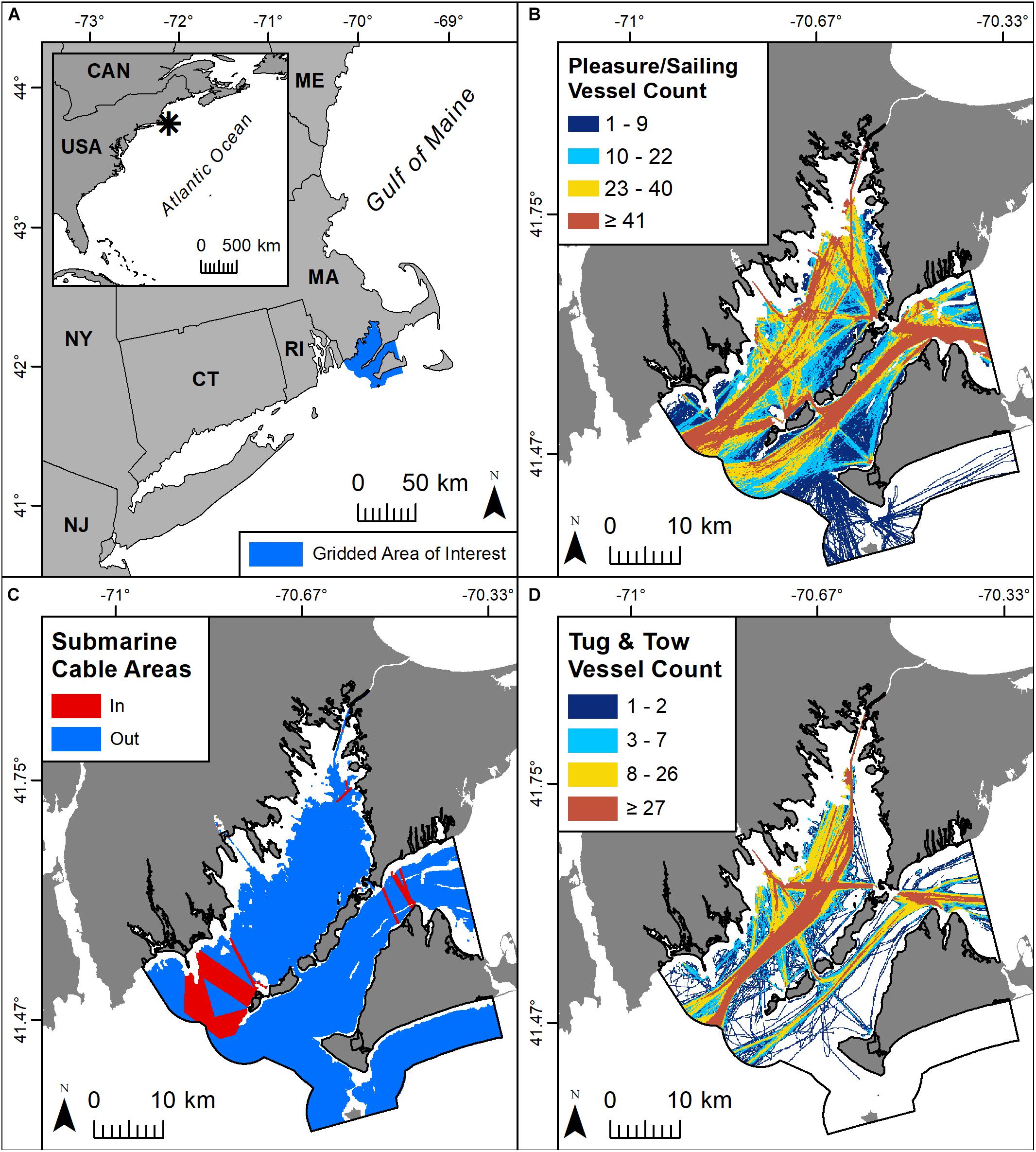
Figure 1. (A) Area of interest (133,776 ha) located in the state waters of Massachusetts, United States. (B) Pleasure and sailing vessel traffic sum of transits per 1 ha for 2017. (C) Submarine cable area presence (in) or absence (out) for each 1 ha grid cell. (D) Tug and tow vessel traffic sum of transits per 1 ha for 2017.

TABLE 1

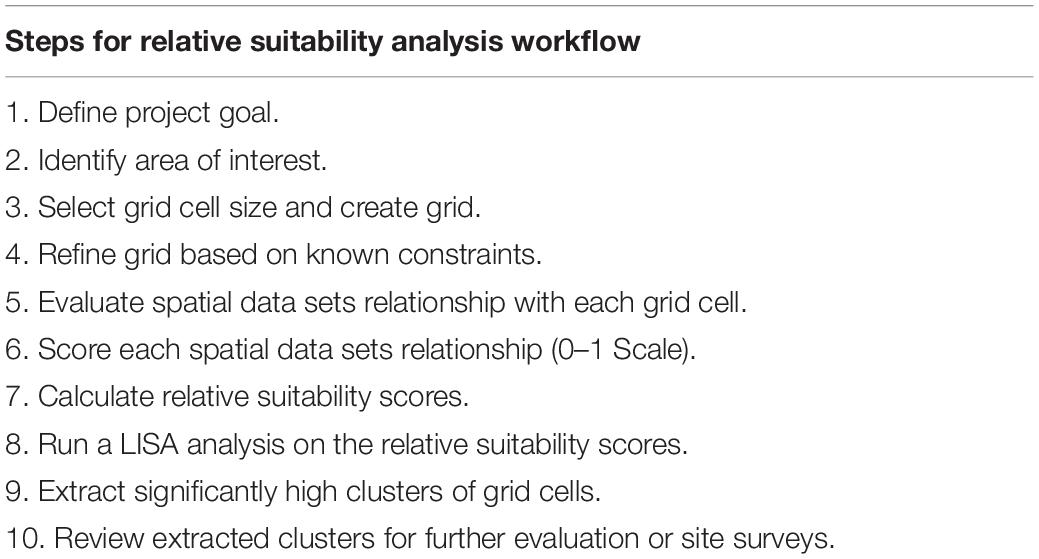
Table 1. Generalized steps performed for the relative suitability analysis, including the Local Indicator of Spatial Association (LISA) analysis.

With the project goal of siting a mussel longline farm and target geography identified, a grid with 1 ha grid cells (100 m by 100 m) was established for an area of interest, containing a total of 133,776 grid cells (Figure 1A). Cell size for the grid was determined based on the resolution of available spatial data for the analysis, inherent spatial variability of the data, and an industry-standard farm footprint size (Hengl, 2006). Grid cells shallower than 10 m were removed, leaving 98,369 grid cells within the acceptable depth range for this aquaculture siting exercise. Spatial data sets containing potential space-use conflicts with marine aquaculture operations, such as active military areas, maritime navigation, ocean industries, and natural resource management, were collated (Table 2 and Figures 1B–D). Data sets were individually assigned a score ranging from 0 (low suitability) to 1 (high suitability) determined by its compatibility with mussel longlines (Table 2).

TABLE 2

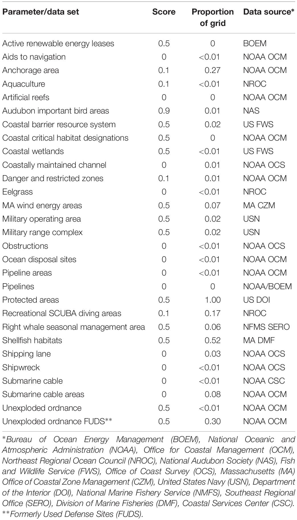
Table 2. Discrete spatial data sets included in the relative suitability analysis with scores ranging from 0 (low suitability) to 1 (high suitability) and proportion of grid cells that the parameter is present in along with the data source.

Each data set was subsequently evaluated to determine if a spatial data set was present or absent within each grid cell. For example, a shipping lane was considered to be present if it intersected a grid cell, and that grid cell would receive a score of 0. For continuous data, such as bathymetry, fishing effort, and sediment grain size, the mean value for each grid cell was calculated and scores were assigned based on operational constraints associated with mussel longlines (e.g., low suitability scores were assigned for areas corresponding with high fishing effort because of the potential for space-use conflict; Tables 3, 4). Vessel traffic from 2017 was categorized by type, and the sum of vessel transits per grid cell was calculated². The 25th, 50th, and 75th, percentiles for each vessel type were calculated for the values in the grid and used to create and categorize the scoring schema (Tables 5, 6). Any grid cell that contained a data set with a score of 0 was considered to be unsuitable regardless of the other scores as that single conflict is completely incompatible for siting. All data sets were integrated by summing all individual scores for each grid cell across all data sets and dividing the sum by the total number of data sets, providing a proportion from 0 to 1, with 0 representing “low suitability” and 1 representing “high suitability” relative to other grid cells. This final proportion provides the relative suitability of that cell to all other grid cells in the area of interest.

TABLE 3

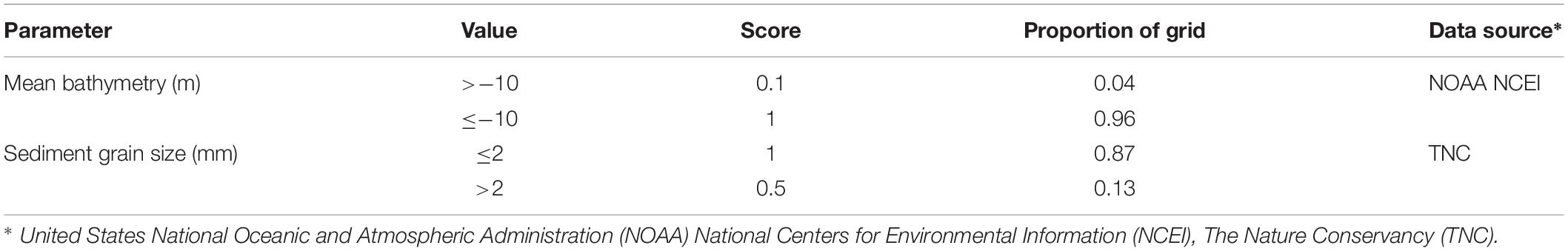
Table 3. Continuous spatial data sets included in the relative suitability analysis with scores ranging from 0 (low suitability) to 1 (high suitability) and proportion of grid cells that the parameter is present in.

TABLE 4

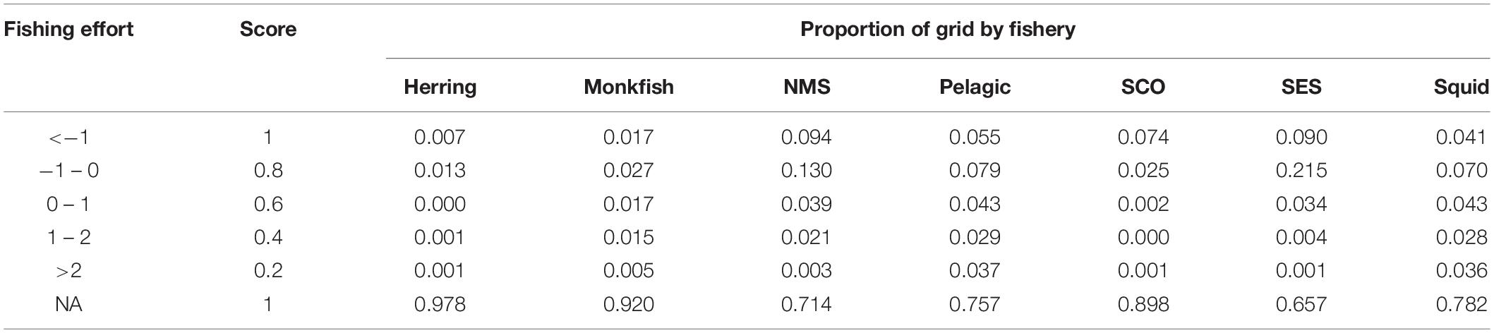
Table 4. Commercial fishing effort 2015–2016 Vessel Monitoring System (VMS) derived (Northeast Regional Ocean Council 2019) categories and scoring schema ranging from 0 (low suitability) to 1 (high suitability), and the proportion of grid cells in each category by fishery (NMS = Multispecies groundfish, Pelagic includes mackerel, squid, and herring, SCO = Quahog, SES = Scallop).

TABLE 5

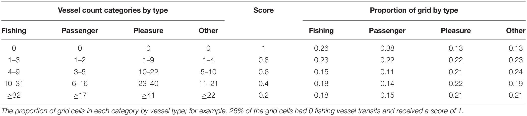
Table 5. Automatic Identification System (AIS) vessel counts by vessel type categories is the count of vessels that passed through a grid cell over the course of 2017 with the corresponding scores ranging from 0 (low suitability) to 1 (high suitability).

TABLE 6

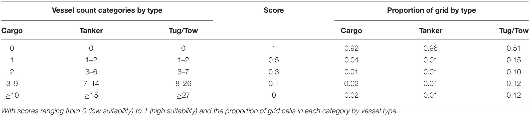
Table 6. Larger vessels with limited maneuverability associated with established shipping lanes from the 2017 Automatic Identification System (AIS) data.

A LISA analysis, which is used to identify statistically significant clusters and outliers within a data set, is then performed on the final proportion of the relative suitability analysis (Anselin, 1995). Esri ArcGIS Pro’s “Cluster and Outlier Analysis” tool was used to perform the LISA analysis (ESRI, 2019)³. The inverse distance spatial conceptualization with a 100 m search distance is used as it includes all grid cells; however, proximal cells have more influence than distant cells. Row standardization, application of a false discovery rate correction, and 999 iterations were all applied for more conservative and robust results. Statistically significant clusters of the highest suitable scores were identified, and any clusters smaller than 20 ha were excluded. A minimum size of 20 ha was used as smaller mussel farms have less economic sustainability and less flexibility for optimal farm configuration (Ahsan and Roth, 2010; Rosland et al., 2011). The LISA analysis is similar to the Getis–Ord Gi^∗ statistic, but in addition to identifying significant high and low clusters, this method identifies outliers (Getis and Ord, 1992; Anselin, 1995). Knowledge of outliers is useful when interpreting results of a MCDA as it highlights areas that may need to be avoided when identifying suitable locations for an aquaculture operation. For example, a sewage discharge pipe or piece of unexploded ordnance may be surrounded by otherwise suitable locations.

Case Study 2: Incremental Spatial Autocorrelation Analysis With Moran’s I

OceanReports enables the public to explore an ocean neighborhood by drawing a polygon anywhere within the United States Exclusive Economic Zone (EEZ) to visualize spatial data within that polygon. An immediate report is provided that includes location-based, regulatory, abiotic, biotic, cultural, and geophysical characteristics specific to the user-defined area. Within the Oceanographic and Biophysical information section of the tool, descriptive statistics from a variety of remotely sensed oceanographic data sets are generated for the custom area (Figure 2A). A user could draw a polygon to inspect and visualize a large area (e.g., the East Coast of the United States), however, the summary statistics of oceanographic data for this expansive area may provide inconsequential information. On the other hand, drawing a smaller polygon would produce more useful localized descriptive statistics of oceanographic parameters for MSP. To address this issue maximum area thresholds were developed for all oceanographic data sets by identifying the amount of area at which spatial dependence or clustering was the most pronounced using an incremental spatial autocorrelation analysis with Moran’s I. OceanReports will not return descriptive statistics for an oceanographic variable if the user-drawn area is greater than the maximum area threshold for that data set. Rather, the tool informs the user to draw a smaller area to receive summary statistics for that variable (Figure 2B). Thus, the likelihood of a user receiving meaningless or misrepresentative summary statistics is reduced.

FIGURE 2

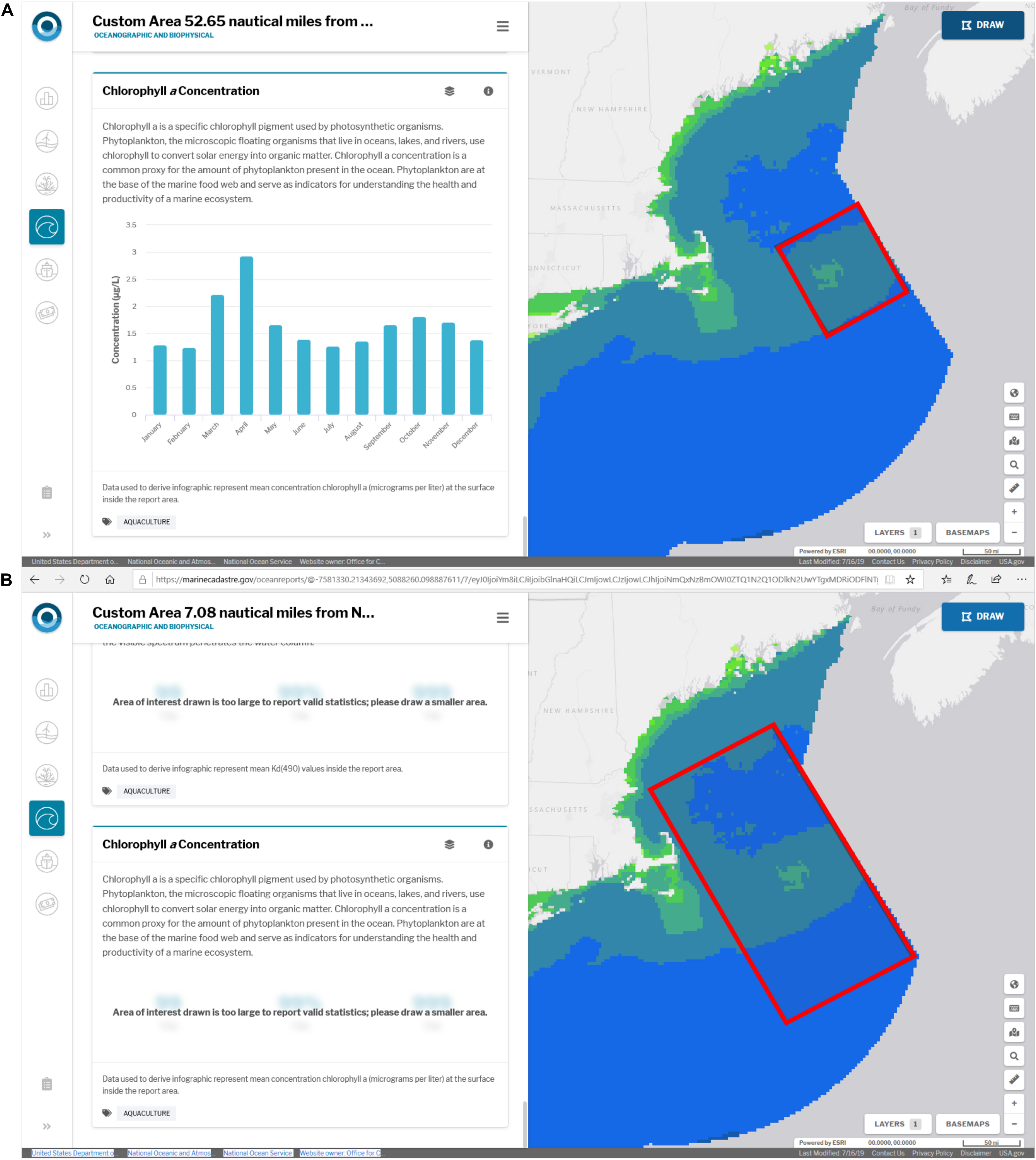
Figure 2. Example output from OceanReports providing (A) descriptive statistics for a number of oceanographic variables based on a custom drawn area and (B) an error message indicating the maximum area threshold has been exceeded.

For this case study, long-term monthly climatologies of remotely sensed chlorophyll a, SST, and current speed, were evaluated within the northeast region of the United States, including state waters to the 200 nm federal waters boundary of the EEZ (Table 7). These three environmental variables are commonly used in siting analyses for marine aquaculture (Radiarta et al., 2008; Snyder et al., 2017; Tung and Son, 2019). Monthly climatologies of surface chlorophyll a concentrations produced by the National Aeronautics and Space Administration (NASA) MODIS-Aqua from July 2002 to February 2019 provide insight into an area’s potential food availability (i.e., phytoplankton biomass) or possible nutrient loading (Gentry et al., 2017; NASA Goddard Space Flight Center, 2018; Theuerkauf et al., 2019). Monthly climatologies of water temperature and current magnitude from October 1992 to December 2012 were derived from the three-dimensional, physical oceanographic Hybrid Coordinate Ocean Model (HYCOM) and Navy Coupled Ocean Data Assimilation (NCODA) 1/12° reanalysis daily 1200 hr measurement (Bleck et al., 2002; Halliwell, 2004). Water temperature is critical for evaluating optimal growth ranges, approximate harvest times, and potential thermal stress thresholds for finfish, shellfish, and macroalgae aquaculture (Gentry et al., 2017). Oceanographic current speed is important to consider when siting aquaculture as well, and is useful for understanding shellfish food availability, equipment limitations, and fish welfare (Ferreira et al., 2007; Huang et al., 2008; Jónsdóttir et al., 2019).

TABLE 7

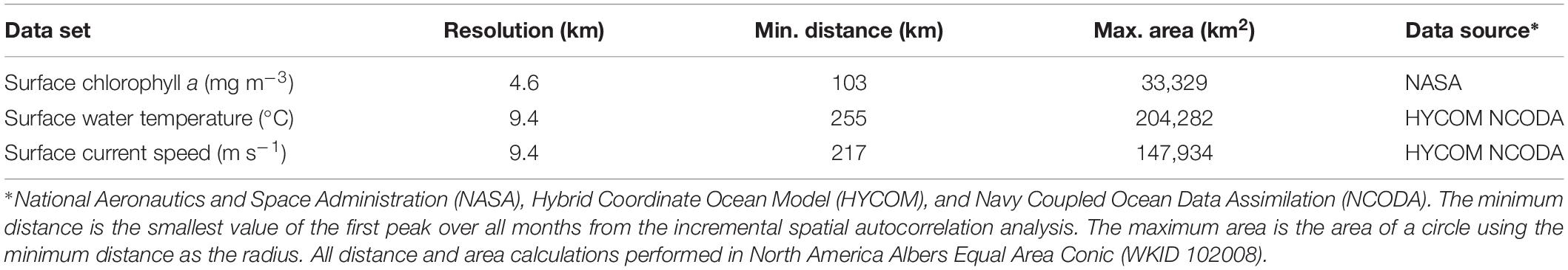
Table 7. Oceanographic data sets examined with units, spatial resolution, and source of data.

An incremental spatial autocorrelation analysis using the global Moran’s I spatial autocorrelation index with a fixed distance spatial conceptualization was performed for each monthly climatology using the “spdep” library in R v3.6.1 (R Core Team, 2019). An incremental spatial autocorrelation analysis calculates the Moran’s I index and z score at multiple distances for a single data set. The fixed distances analyzed were derived from each possible distance between one data point and all other data points. For example, if 100 possible distances existed in a data set, Moran’s I index would be run 100 times or once for each distance. The resulting z scores are then plotted by distance, rather than using the Moran’s I index value, as the z scores allow for a standardized comparison of significance by distance (i.e., larger positive z scores have more significant clustering). The distances at the first peak and maximum peak were identified for each plot. The first peak indicates smaller significant clustering and the maximum peak indicates the distance that clustering or spatial autocorrelation was most significant in the data set. The distance of the first z score peak, which also was the maximum peak for all data sets, provided a radius, and the standard formula for the area of a circle was performed to calculate an area for each monthly climatology.

OceanReports provides descriptive statistics for each month in a user drawn area, and therefore, the smallest area threshold or the most conservative estimate was chosen as the threshold for each oceanographic parameter. Using the smallest area threshold from all monthly climatologies assists in ensuring a user defined area contains appropriate summary statistics within the online DST. A temporal component was not included within this spatial dependence analysis, because the objective was simply to identify the smallest or most conservative area as determined by the distance at which spatial clustering was most significant. Therefore each monthly climatology was treated as an independent data set. Methodologies for using a spatio-temporal Moran’s I index have been developed, and examine how spatial dependence patterns change over time or at different time scales. For example, Shen et al. (2016) demonstrate how a temporally detrended global spatio-temporal Moran’s I index, which accounts for temporal data that is not stationary, may be used to examine changes in the spatial and temporal dependence of daily precipitation data sets in China.

Results

Case Study 1: MCDA With Cluster and Outlier Analysis

The MCDA identified roughly 26% of the area of interest as unsuitable (i.e., received a score of 0) for mussel longlines. Vessel traffic, specifically “tug and tow” vessel traffic, and submarine cable areas removed the greatest amount of suitable area (Figures 1C,D). The remaining 74% varied in levels of suitability (i.e., suitability scores ranging from >0 to 1; Figure 3A). The LISA analysis identified statistically significant highly suitable clusters with at least 20 ha of a contiguous area within 17% of the total area (Figure 3D). Within these highly suitable grid cells, the most considerable constraints were “pleasure and sailing craft” and “other” vessel traffic, as well as the presence of protected areas and shellfish habitats (Figure 1B; Tables 2, 5). A few outliers with unsuitable cells adjacent to highly suitable cells were identified; these were either aids to navigation or other navigational obstructions (e.g., shipwrecks; Figure 4).

FIGURE 3

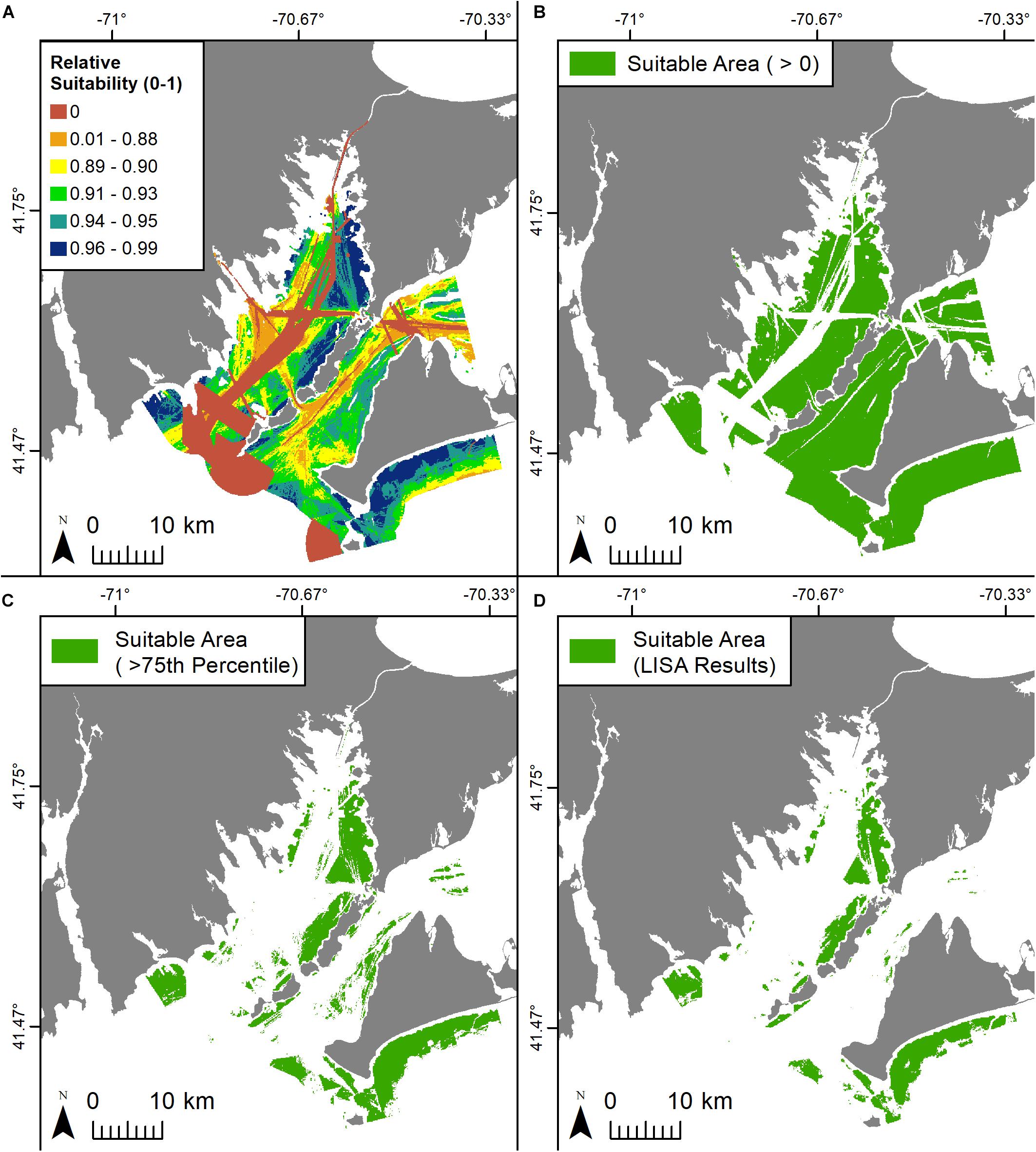
Figure 3. (A) The relative suitability analysis results. A score of 0 indicates completely unsuitable, while a score closer to 1 indicates higher relative suitability with aquaculture. (B) Suitable area using a traditional binary exclusion analysis (Suitability score >0). (C) Suitable area using a threshold (Suitability score >75th percentile). (D) Highly suitable areas greater than 20 ha based on the Local Indicator of Spatial Association (LISA) analysis using the relative suitability score.

FIGURE 4

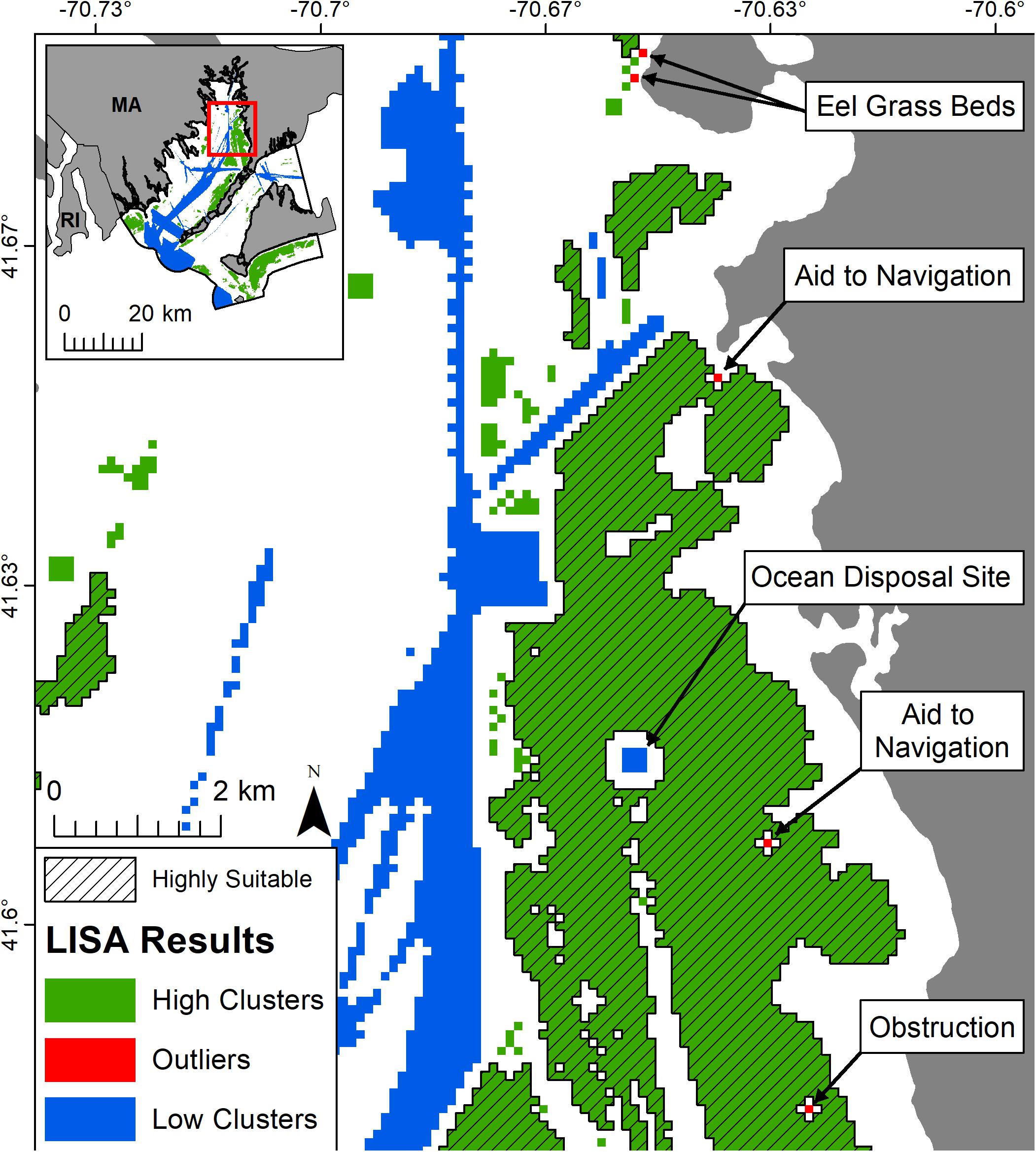
Figure 4. Results of the Local Indicator of Spatial Association (LISA) analysis displaying the highly suitable high clusters, with outliers and low clusters. Groups of high clusters less than 20 ha were not considered highly suitable.

Case Study 2: Incremental Spatial Autocorrelation Analysis With Moran’s I

The Moran’s I z scores plotted by distance identified the distances at which clustering was most significant for the three oceanographic variables presented. Throughout the monthly climatologies, the distances of the first peak for chlorophyll a z scores ranged from 103 to 124 km, with the smallest distance of 103 km occurring in April, May, and July (Figures 5A,B). Water temperature distances had a range of 255 to 453 km, with the shortest distance in February at 255 m (Figures 5C,D). The first peak distances for current magnitude ranged from 217 to 245 km, exhibiting the shortest distance of 217 km in July, August, and October (Figures 5E,F). Plotting the distance values at the first peak for all variables by month demonstrates how the sizes of clusters within a data set fluctuates throughout the year. The smallest distance is used to calculate the maximum area threshold used by OceanReports (Table 7 and Figure 6).

FIGURE 5

Figure 5. (A) Chlorophyll a z scores plotted by distance band for each month, vertical red dotted line indicates the smallest distance of the first peak, 103 km. (B) June chlorophyll a climatology with the red circle having an area of 33,329 km². (C) Sea Surface Temperature (SST) z scores plotted by distance band for each month, vertical red dotted line indicates the smallest distance of the first peak, 255 km. (D) February SST climatology, red circle with area of 204,282 km². (E) Surface current speed z scores plotted by distance band for each month, vertical red dotted line indicates the smallest distance of the first peak, 217 km. (F) October current speed climatology, red circle with area of 147,934 km².

FIGURE 6

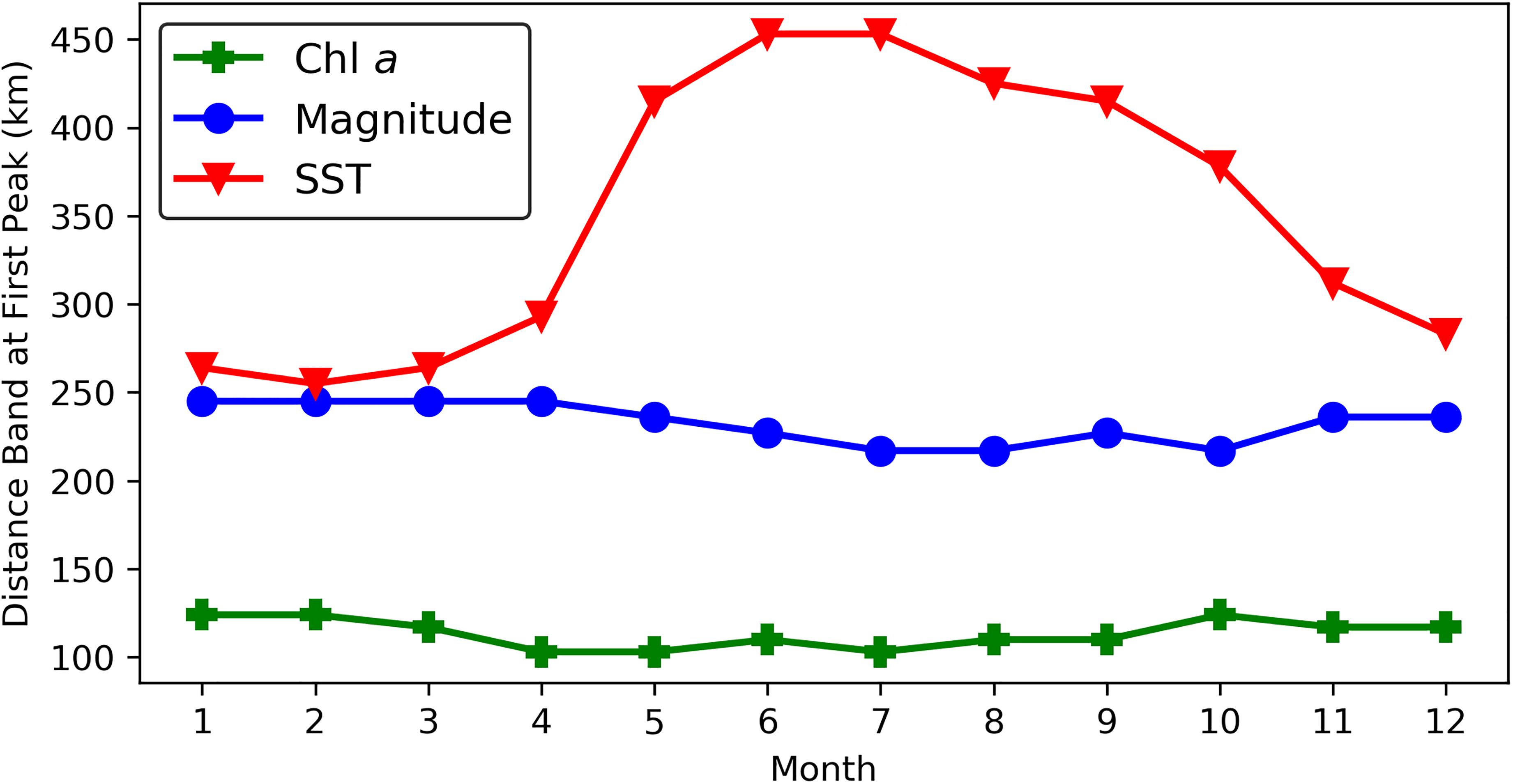
Figure 6. Distance band at first peak by month for the three oceanographic variables examined. The month with the smallest minimum distance band was used to calculate the maximum area threshold to be used within the decision support tool, OceanReports.

Discussion

As global interest in “blue economy” initiatives and strategies expands, the MSP framework and associated geospatial analyses will be increasingly relied upon to minimize anthropogenic impacts on the ocean environment and space-use conflicts (Golden et al., 2017). Spatial autocorrelation approaches improve the reliability, rigor, and utility of the decision support guidance provided by MSP analyses. The two presented case studies showcase the utility of spatial autocorrelation analyses to (1) inform identification of clusters of highly suitable ocean areas for marine aquaculture that minimizes space-use conflict, and (2) prevent users from receiving misrepresentative summary statistics for oceanographic parameters within an online DST by defining maximum area thresholds. The potential applications of spatial autocorrelation analyses to help resource managers and industry better understand and apply these analyses are diverse and hold great promise to reduce uncertainty and provide a data-driven approach to the interpretation of results.

The first case study successfully identifies areas that are completely unsuitable (received a score of 0) for mussel longline aquaculture. Submarine cable areas, ocean disposal sites, and other navigational constraints were present; however, the “cargo”, “tanker,” and “tug and tow” vessel traffic in transit to the Cape Cod Canal in the area of interest was the most considerable constraint (Figure 1D and Table 6). Quantifying vessel traffic from AIS land-based or satellite data ensures vessel-related considerations are adequately characterized within spatial analyses to reduce potential conflict with other ocean industries, such as shipping, fishing, or recreation (Metcalfe et al., 2018; Tlusty et al., 2018). Any grid cells with values greater than 0 in the relative suitability analysis are considered negotiable ocean space.

The LISA analysis identified statistically significant clusters of cells that have low conflict relative to other grid cells, which is an improvement over other methods. Typically, the results of a MCDA for marine aquaculture (e.g., suitability maps) are visually and qualitatively assessed to identify areas with high potential for compatibility with marine aquaculture (Figure 3A). The simplest approach is to exclude areas that were completely unsuitable and evaluate all other areas by examining constraints (Figure 3B). Additionally, a threshold may be applied to the score; for example, grid cell values greater than the 75th percentile could be considered highly suitable and examined apart from the other grid cells (Figure 3C). Both approaches may aid in identifying potential areas, however, simply excluding unsuitable areas generally leaves a large area that must be sifted through, cell by cell, to identify sites. Establishing a score threshold reduces the amount of area; however, choosing a “good” suitability score threshold may be difficult to establish and justify.

Use of a LISA analysis identified 17% of the total area as having statistically higher suitable scores relative to the other grid cells (Figure 3D) and identified outliers that should be avoided (Figure 4). Compared to the two other approaches described, the LISA analysis identified a smaller area by means of spatial statistics, which provides decision makers and coastal managers increased confidence when examining the results of a spatial planning analysis. Regardless of the analysis used, further review of the highly suitable locations is required for the creation and evaluation of alternative sites for any marine aquaculture operation. The benefit of the LISA analysis is the standardized process and method for identifying statistically significant clusters, which serves as a basis for discussion with local managers and stakeholders.

Regardless of the methods used to calculate the suitability scores, a LISA analysis can be used to identify statistically significant clusters of high values and detect outliers. Methods range from a simple exclusion analysis (i.e., excluding areas representing known constraints) to more complicated MCDA suitability modeling that include weighted variables. For example, Pérez et al. (2005) used a weighted linear combination method for development of a MCDA whereby decision makers assign weights to each factor considered within the analysis, with the final output being a weighted average. Weighted variables provides more confidence in determining what a “good” score is; however, setting a score threshold (e.g., 0.80) and interpreting the results may still be challenging. Thus, a LISA analysis provides a robust approach that may be used to guide interpretation of suitability analysis outputs by identifying statistically significant clusters and outliers. In the presented case study, all data sets were equally weighted, however, if weights were applied, standardized methods of collecting stakeholder input or expert knowledge should be used over arbitrary assignment of values (Alexander et al., 2012; Klain and Chan, 2012; Teniwut et al., 2019).

Similar to other MSP analyses, the relative suitability and LISA analyses presented here have various assumptions and limitations. Marine aquaculture spatial planning projects typically rely upon the best available data for planning despite known data limitations and gaps (Longdill et al., 2008). For example in this case study, the most recent and best available vessel traffic data was used, however, vessels not required to carry an AIS transponder were not represented. Using the best available data and noting any assumptions or limitations can improve trust and reliability in the results, while also highlighting future data needs. Appropriate grid cell size and search distances are required, and should be based on the data and size of area being examined, as using inappropriate sizes or distances may provide limited results. Additionally a relative suitability analysis was performed, which means a highly suitable cluster does not guarantee a location is highly suitable for aquaculture, only that it is highly suitable relative to the other locations examined. Regardless of the type of spatial planning analysis, onsite surveys will be required to ensure a site’s compatibility with marine aquaculture.

Within the second case study, the distance at which the Moran’s I index z score first peaked for chlorophyll a, SST, and current speed, was identified for each month. These distances are consistent with known regional oceanographic patterns. Monthly climatological values for chlorophyll a, which is frequently used as a surrogate variable for phytoplankton biomass, displayed a general pattern of phytoplankton blooms in early spring and summer, which is typical in the North Atlantic (Friedland et al., 2016; Figure 5A). The surface water temperature displayed higher clustering in the winter months when temperature differences increase among the estuaries, the Gulf of Maine, and the Gulf Stream, while in the summer months, the water temperatures are more uniform throughout the northeast region (Shearman and Lentz, 2010; Figure 5C). Surface current speeds had higher clustering in late summer, which may be related to increased storm activity (Fewings et al., 2008; Figure 5E). The area threshold for each oceanographic parameter was calculated by using the smallest distance observed over the 12 months (Figure 6 and Table 7). The incorporation of these into OceanReports lessen the possibility of a user receiving potentially misrepresentative descriptive statistics.

Alternative methods of establishing maximum area thresholds exist, but the target audience and industry of the DST should be used to guide any thresholds. For example, a DST built solely for marine aquaculture planning could use an area threshold determined by industry or regulatory standards. Since OceanReports was designed for a variety of industries with varying needs, determining area thresholds that accommodate different user groups was required. The incremental spatial autocorrelation analysis is able to accomplish this by producing thresholds for each oceanographic variable based on cluster sizes within that data set. For example, different descriptive statistics (i.e., changes in the mean concentration of chlorophyll a) are obtained as the area of interest changes, and once the area exceeds the threshold the results begin to mean less for localized planning (Figures 7A,B). When the custom area is smaller than the threshold a user may still receive inconsequential descriptive statistics for an oceanographic variable within OceanReports, because of where and how the area is drawn. However, the use of a maximum area threshold reduces the likelihood of this occurring. Inclusion of maximum area thresholds for oceanographic parameters used by OceanReports provides guidance for users, especially those unfamiliar with descriptive statistics and oceanographic parameters, during exploratory analysis of an area.

FIGURE 7

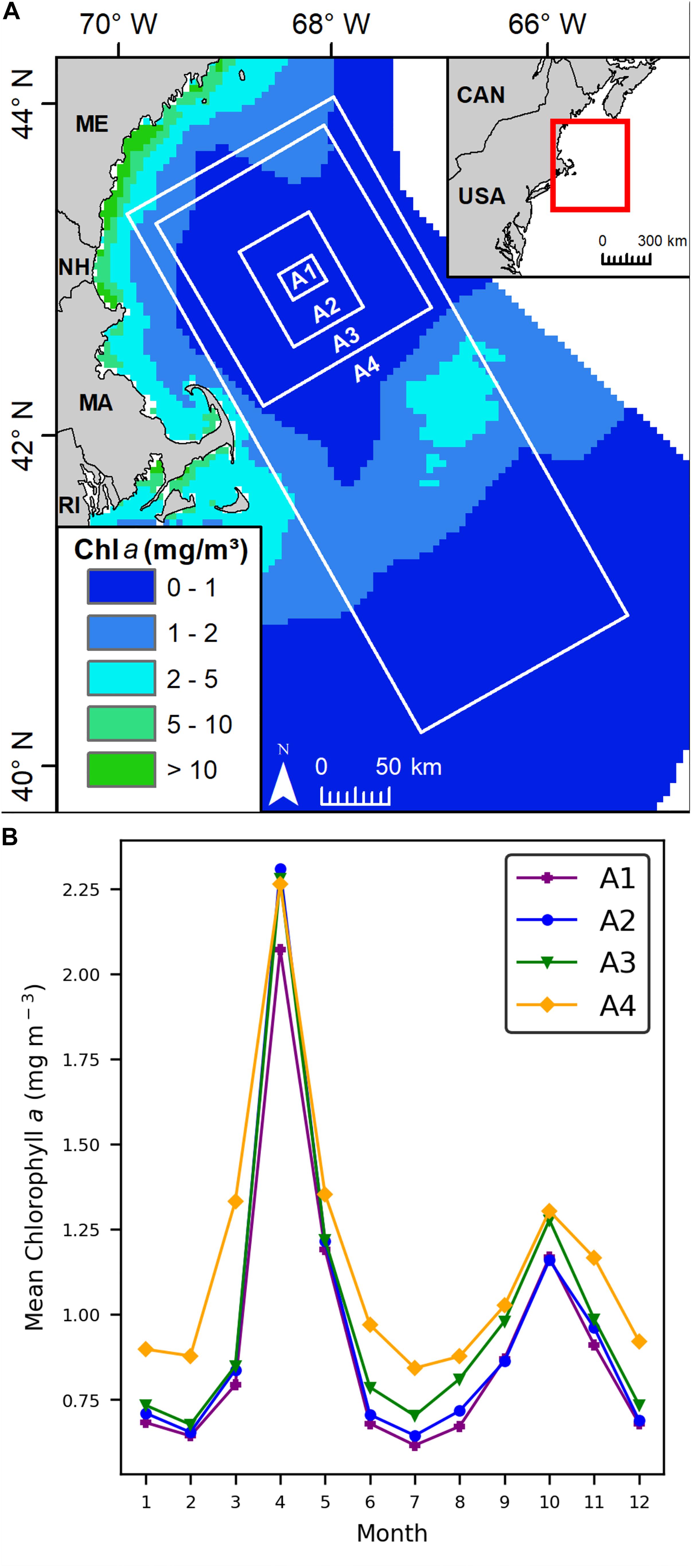
Figure 7. (A) Example of different hypothetical areas of interest (A1 = 625 km², A2 = 4,778 km², A3 = 22,428 km², A4 = 76,995 km²). (B) Mean chlorophyll a concentration for each of the area sizes, A1, A2, A3, and A4.

Several other pragmatic applications of spatial autocorrelation analyses may be assimilated into the MSP process for marine aquaculture, such as spacing of environmental monitoring stations or farms. Key environmental variables, such as nutrient input and impact to benthic habitat, may require monitoring to be performed (Holmer et al., 2008). Environmental variables with significant spatial autocorrelation (i.e., High clustering of a variable) around a farm should be sampled at additional locations, while variables with no significant spatial autocorrelation (i.e., Random distribution of a variable) require less spatial coverage for monitoring (Foster et al., 2018). The spacing and distance of sample points may be calculated after initial survey data has been collected, using a semivariogram or an incremental spatial autocorrelation analysis. The resulting distances may be used to space farm sites as well. As marine aquaculture development continues, so too will the need for rigorous analysis to provide assurance to stakeholders and coastal managers that a location is suitable.

Conclusion

The marine aquaculture industry needs efficient, objective, and accessible spatial planning tools in order to responsibly and efficiently plan for aquaculture. In the first case study, the relative suitability analysis and LISA analysis identified highly suitable locations for a hypothetical mussel longline farm in 17% of the area examined. The use of these analyses to statistically identify high clusters provides confidence and reliability for industry, coastal managers, and stakeholders, that these locations are the most suitable for a mussel longline farm in the area of interest. The second case study calculated maximum area thresholds using an incremental spatial autocorrelation analysis for chlorophyll a, SST, and current speed, to be used within OceanReports. These area thresholds were determined by the distance that spatial dependence or clustering was greatest within each data set, rather than arbitrarily assigning an area threshold. These maximum area thresholds provide users guidance and descriptive statistics that are meaningful for MSP activities. Incorporating spatial autocorrelation analyses into the MSP process improves efficiency and confidence when planning for marine aquaculture.

Data Availability Statement

The datasets generated for this study are available upon request to the corresponding author.

Author Contributions

JJ, ST, and LW conceived the idea for the manuscript and developed the methods. JJ executed the analysis. JJ, ST, LW, and JM reviewed and discussed the results. JJ, ST, LW, and JM wrote the manuscript. JM reviewed the final manuscript.

Funding

This work was supported by the NOAA National Ocean Service, National Centers for Coastal Ocean Science; NOAA National Marine Fisheries Service, Office of Aquaculture; and Department of Energy, Advanced Research Projects Agency-Energy.

Conflict of Interest

JJ and LW are employees of the company CSS, Inc., and are under contract to NOAA.

The remaining authors declare that the research was conducted in the absence of any commercial or financial relationships that could be construed as a potential conflict of interest.

Acknowledgments

The authors thank Samantha Binion-Rock and Daniel Martin who provided comments and input to an early version of the manuscript. The authors also thank the NOAA/NMFS Office of Aquaculture, NOAA National Centers for Coastal Ocean Service (NCCOS) and the DOE ARPA-E program for support of this publication.

Footnotes

1. ^ https://coast.noaa.gov/digitalcoast/tools/ort.html
2. ^ https://marinecadastre.gov/ais/
3. ^ https://pro.arcgis.com/en/pro-app/tool-reference/spatial-statistics/cluster-and-outlier-analysis-anselin-local-moran-s.htm

References

Aguilar-Manjarrez, J., Soto, D., and Brummett, R. (2017). Aquaculture Zoning, Site Selection and Area Management Under the Ecosystem Approach to Aquaculture. A Handbook. Italy: Food and Agriculture Organization of the United Nations.

Google Scholar

Ahsan, D. A., and Roth, E. V. A. (2010). Farmers’ perceived risks and risk management strategies in an emerging mussel aquaculture industry in Denmark. Mar. Resour. Econ. 25, 309–323. doi: 10.5950/0738-1360-25.3.309

CrossRef Full Text | Google Scholar

Alexander, K. A., Janssen, R., Arciniegas, G., O’Higgins, T. G., Eikelboom, T., and Wilding, T. A. (2012). Interactive marine spatial planning: siting tidal energy arrays around the Mull of Kintyre. PLoS One 7:e0030031. doi: 10.1371/journal.pone.0030031

PubMed Abstract | CrossRef Full Text | Google Scholar

Anselin, L. (1995). Local indicators of spatial association—LISA. Geog. Anal. 27, 93–115. doi: 10.1186/s12942-017-0119-3

PubMed Abstract | CrossRef Full Text | Google Scholar

Bleck, R., Halliwell, G., Wallcraft, A., Carroll, S., Kelly, K., and Rushing, K. (2002). HYbrid Coordinate Ocean Model (HYCOM) User’s Manual: Details of the Numerical Code. HYCOM. Available at: https://www.hycom.org/attachments/063_hycom_users_manual.pdf (accessed June 3, 2019).

Google Scholar

Brager, L. M., Cranford, P. J., Grant, J., and Robinson, S. M. (2015). Spatial distribution of suspended particulate wastes at open-water Atlantic salmon and sablefish aquaculture farms in Canada. Aquacult. Environ. Interact. 6, 135–149. doi: 10.3354/aei00120

CrossRef Full Text | Google Scholar

Bwadi, B. E., Mustafa, F. B., Ali, M. L., and Bhassu, S. (2019). Spatial analysis of water quality and its suitability in farming giant freshwater prawn (Macrobrachium rosenbergii) in Negeri Sembilan region, Peninsular Malaysia. Singapore J. Trop. Geog. 40, 71–91. doi: 10.1111/sjtg.12250

CrossRef Full Text | Google Scholar

Collie, J. S., Beck, M. W., Craig, B., Essington, T. E., Fluharty, D., Rice, J., et al. (2013). Marine spatial planning in practice. Estuarine Coastal Shelf Sci. 117, 1–11.

Google Scholar

Dapueto, G., Massa, F., Costa, S., Cimoli, L., Olivari, E., Chiantore, M., et al. (2015). A spatial multi-criteria evaluation for site selection of offshore marine fish farm in the Ligurian Sea, Italy. Ocean Coastal Manage. 116, 64–77. doi: 10.1016/j.ocecoaman.2015.06.030

CrossRef Full Text | Google Scholar

Diniz-Filho, J. A. F., Bini, L. M., and Hawkins, B. A. (2003). Spatial autocorrelation and red herrings in geographical ecology. Glob. Ecol. Biogeogr. 12, 53–64. doi: 10.1046/j.1466-822x.2003.00322.x

CrossRef Full Text | Google Scholar

Douvere, F. (2008). The importance of marine spatial planning in advancing ecosystem-based sea use management. Mar. Policy 32, 762–771. doi: 10.1016/j.marpol.2008.03.021

CrossRef Full Text | Google Scholar

ESRI (2019). ArcGIS Pro: Release 2.4.0. Redlands, CA: Environmental Systems Research Institute.

Google Scholar

Ferreira, J. G., Hawkins, A. J. S., and Bricker, S. B. (2007). Management of productivity, environmental effects and profitability of shellfish aquaculture—the Farm Aquaculture Resource Management (FARM) model. Aquaculture 264, 160–174. doi: 10.1016/j.aquaculture.2006.12.017

CrossRef Full Text | Google Scholar

Fewings, M., Lentz, S. J., and Fredericks, J. (2008). Observations of cross-shelf flow driven by cross-shelf winds on the inner continental shelf. J. Phys. Oceanogr. 38, 2358–2378. doi: 10.1175/2008jpo3990.1

CrossRef Full Text | Google Scholar

Foster, S. D., Monk, J., Lawrence, E., Hayes, K. R., Hosack, G. R., and Przeslawski, R. (2018). “Statistical considerations for monitoring and sampling,” in Field Manuals for Marine Sampling to Monitor Australian Waters, eds R. Przeslawski, and S. Foster, (Canberra ACT: National Environmental Science Programme, Marine Biodiversity Hub), 23–41.

Google Scholar

Friedland, K. D., Record, N. R., Asch, R. G., Kristiansen, T., Saba, V. S., Drinkwater, K. F., et al. (2016). Seasonal phytoplankton blooms in the North Atlantic linked to the overwintering strategies of copepods. Elem. Sci. Anth. 4:000099. doi: 10.12952/journal.elementa.000099

CrossRef Full Text | Google Scholar

Gentry, R. R., Lester, S. E., Kappel, C. V., White, C., Bell, T. W., Stevens, J., et al. (2017). Offshore aquaculture: spatial planning principles for sustainable development. Ecol. Evol. 7, 733–743. doi: 10.1002/ece3.2637

PubMed Abstract | CrossRef Full Text | Google Scholar

Getis, A., and Ord, J. K. (1992). The analysis of spatial association by use of distance statistics. Geog. Anal. 24, 189–206. doi: 10.1111/j.1538-4632.1992.tb00261.x

CrossRef Full Text | Google Scholar

Gimpel, A., Stelzenmüller, V., Grote, B., Buck, B. H., Floeter, J., Núñez-Riboni, I., et al. (2015). A GIS modelling framework to evaluate marine spatial planning scenarios: Co-location of offshore wind farms and aquaculture in the German EEZ. Mar. Policy 55, 102–115. doi: 10.1016/j.marpol.2015.01.012

CrossRef Full Text | Google Scholar

Golden, J. S., Virdin, J., Nowacek, D., Halphin, P., Bennear, L., and Patil, P. G. (2017). Making sure the blue economy is green. Nat. Ecol. Evol. 1:17. doi: 10.1038/s41559-016-0017

PubMed Abstract | CrossRef Full Text | Google Scholar

Halliwell, G. R. (2004). Evaluation of vertical coordinate and vertical mixing algorithms in the HYbrid-Coordinate Ocean Model (HYCOM). Ocean Model. 7, 285–322. doi: 10.1016/j.ocemod.2003.10.002

CrossRef Full Text | Google Scholar

Hawkins, B. A., Diniz-Filho, J. A. F., Mauricio Bini, L., De Marco, P., and Blackburn, T. M. (2007). Red herrings revisited: spatial autocorrelation and parameter estimation in geographical ecology. Ecography 30, 375–384. doi: 10.1111/j.2007.0906-7590.05117.x

CrossRef Full Text | Google Scholar

Hengl, T. (2006). Finding the right pixel size. Comput. Geosci. 32, 1283–1298. doi: 10.1016/j.cageo.2005.11.008

CrossRef Full Text | Google Scholar

Holmer, M., Hansen, P. K., Karakassis, I., Borg, J. A., and Schembri, P. J. (2008). “Monitoring of environmental impacts of marine aquaculture,” in Aquaculture in the Ecosystem, eds M. Holmer, K. Black, C. M. Duarte, N. Marbà, and I. Karakassis, (Berlin: Springer Science & Business Media), 47–85. doi: 10.1007/978-1-4020-6810-2_2

CrossRef Full Text | Google Scholar

Huang, C. C., Tang, H. J., and Liu, J. Y. (2008). Effects of waves and currents on gravity-type cages in the open sea. Aquacult. Eng. 38, 105–116. doi: 10.1016/j.aquaeng.2008.01.003

CrossRef Full Text | Google Scholar

Izumi, K., Ohkado, A., Uchimura, K., Murase, Y., Tatsumi, Y., Kayebeta, A., et al. (2015). Detection of tuberculosis infection hotspots using activity spaces based spatial approach in an urban Tokyo, from 2003 to 2011. PLoS One 10:e0138831. doi: 10.1371/journal.pone.0138831

PubMed Abstract | CrossRef Full Text | Google Scholar

Jónsdóttir, K. E., Hvas, M., Alfredsen, J. A., Føre, M., Alver, M. O., Bjelland, H. V., et al. (2019). Fish welfare based classification method of ocean current speeds at aquaculture sites. Aquacult. Environ. Interact. 11, 249–261. doi: 10.3354/aei00310

CrossRef Full Text | Google Scholar

Klain, S. C., and Chan, K. M. (2012). Navigating coastal values: participatory mapping of ecosystem services for spatial planning. Ecol. Econ. 82, 104–113. doi: 10.1016/j.ecolecon.2012.07.008

CrossRef Full Text | Google Scholar

Kühn, I. (2007). Incorporating spatial autocorrelation may invert observed patterns. Divers. Distrib. 13, 66–69.

Google Scholar

Legendre, P. (1993). Spatial autocorrelation: trouble or new paradigm? Ecology 74, 1659–1673. doi: 10.2307/1939924

CrossRef Full Text | Google Scholar

Lester, S. E., Stevens, J. M., Gentry, R. R., Kappel, C. V., Bell, T. W., Costello, C. J., et al. (2018). Marine spatial planning makes room for offshore aquaculture in crowded coastal waters. Nat. Commun. 9:945. doi: 10.1038/s41467-018-03249-1

PubMed Abstract | CrossRef Full Text | Google Scholar

Longdill, P. C., Healy, T. R., and Black, K. P. (2008). An integrated GIS approach for sustainable aquaculture management area site selection. Ocean Coastal Manag. 51, 612–624. doi: 10.1016/j.ocecoaman.2008.06.010

CrossRef Full Text | Google Scholar

Metcalfe, K., Bréheret, N., Chauvet, E., Collins, T., Curran, B. K., Parnell, R. J., et al. (2018). Using satellite AIS to improve our understanding of shipping and fill gaps in ocean observation data to support marine spatial planning. J. Appl. Ecol. 55, 1834–1845. doi: 10.1111/1365-2664.13139

CrossRef Full Text | Google Scholar

NASA Goddard Space Flight Center (2018). Ocean Ecology Laboratory, Ocean Biology Processing Group. Data from: Moderate-Resolution Imaging Spectroradiometer (MODIS) Aqua chlorophyll data. Greenbelt, MD: NASA OB.DAAC, doi: 10.5067/AQUA/MODIS/L3B/CHL/2018

CrossRef Full Text | Google Scholar

National Marine Fisheries Service [NMFS] (2017). Fisheries of the United States, 2016. U.S. Department of Commerce, NOAA Current Fishery Statistics No. 2016. Available at: https://www.fisheries.noaa.gov/resource/document/fisheries-united-states-2016-report (accessed July 10, 2019).

Google Scholar

Nelson, T. A., and Boots, B. (2008). Detecting spatial hot spots in landscape ecology. Ecography 31, 556–566. doi: 10.1111/j.0906-7590.2008.05548.x

CrossRef Full Text | Google Scholar

Overton, K., Dempster, T., Oppedal, F., Kristiansen, T. S., Gismervik, K., and Stien, L. H. (2018). Salmon lice treatments and salmon mortality in Norwegian aquaculture: a review. Rev. Aquacult. 11, 1398–1417. doi: 10.1111/raq.12299

CrossRef Full Text | Google Scholar

Pérez, O. M., Telfer, T. C., and Ross, L. G. (2005). Geographical information systems-based models for offshore floating marine fish cage aquaculture site selection in Tenerife. Canary Islands. Aquacult. Res. 36, 946–961. doi: 10.1111/j.1365-2109.2005.01282.x

CrossRef Full Text | Google Scholar

Pınarbaşı, K., Galparsoro, I., Borja, Á, Stelzenmüller, V., Ehler, C. N., and Gimpel, A. (2017). Decision support tools in marine spatial planning: present applications, gaps and future perspectives. Mar. Policy 83, 83–91. doi: 10.1016/j.marpol.2017.05.031

CrossRef Full Text | Google Scholar

Puniwai, N., Canale, L., Haws, M., Potemra, J., Lepczyk, C., and Gray, S. (2014). Development of a GIS-based tool for aquaculture siting. ISPRS Int. J. Geo-Inf. 3, 800–816. doi: 10.3390/ijgi3020800

CrossRef Full Text | Google Scholar

R Core Team, (2019). R: A Language and Environment for Statistical Computing. Vienna: R Foundation for Statistical Computing.

Google Scholar

Radiarta, I. N., Saitoh, S. I., and Miyazono, A. (2008). GIS-based multi-criteria evaluation models for identifying suitable sites for Japanese scallop (Mizuhopecten yessoensis) aquaculture in Funka Bay, southwestern Hokkaido. Japan. Aquacult. 284, 127–135. doi: 10.1016/j.aquaculture.2008.07.048

CrossRef Full Text | Google Scholar

Radiarta, I. N., Saitoh, S. I., and Yasui, H. (2011). Aquaculture site selection for Japanese kelp (Laminaria japonica) in southern Hokkaido, Japan, using satellite remote sensing and GIS-based models. ICES J. Mar. Sci. 68, 773–780. doi: 10.1093/icesjms/fsq163

CrossRef Full Text | Google Scholar

Rauner, S., Eichhorn, M., and Thrän, D. (2016). The spatial dimension of the power system: investigating hot spots of smart renewable power provision. Appl. Energy 184, 1038–1050. doi: 10.1016/j.apenergy.2016.07.031

CrossRef Full Text | Google Scholar

Rawson, A., and Rogers, E. (2015). Assessing the impacts to vessel traffic from offshore wind farms in the Thames Estuary. Sci. J. Marit. Univ. Szczecin 43, 99–107.

Google Scholar

Rosland, R., Bacher, C., Strand, Ø, Aure, J., and Strohmeier, T. (2011). Modelling growth variability in longline mussel farms as a function of stocking density and farm design. J. Sea Res. 66, 318–330. doi: 10.1016/j.seares.2011.04.009

CrossRef Full Text | Google Scholar

Rouse, S., Kafas, A., Hayes, P., and Wilding, T. A. (2017). Development of data layers to show the fishing intensity associated with individual pipeline sections as an aid for decommissioning decision-making. Underwater Technol. 34, 171–178. doi: 10.3723/ut.34.171

CrossRef Full Text | Google Scholar

Shearman, R. K., and Lentz, S. J. (2010). Long-term sea surface temperature variability along the U.S. East Coast. J. Phys. Oceanogr. 40, 1004–1017. doi: 10.1175/2009jpo4300.1

CrossRef Full Text | Google Scholar

Shen, C., Li, C., and Si, Y. (2016). Spatio-temporal autocorrelation measures for nonstationary series: a new temporally detrended spatio-temporal Moran’s index. Phys. Lett. A 380, 106–116. doi: 10.1016/j.physleta.2015.09.039

CrossRef Full Text | Google Scholar

Silva, C., Ferreira, J. G., Bricker, S. B., DelValls, T. A., Martín-Díaz, M. L., and Yáñez, E. (2011). Site selection for shellfish aquaculture by means of GIS and farm-scale models, with an emphasis on data-poor environments. Aquaculture 318, 444–457. doi: 10.1016/j.aquaculture.2011.05.033

CrossRef Full Text | Google Scholar

Snyder, J., Boss, E., Weatherbee, R., Thomas, A. C., Brady, D., and Newell, C. (2017). Oyster aquaculture site selection using Landsat 8-derived sea surface temperature, turbidity, and chlorophyll a. Front. Mar. Sci. 4:190. doi: 10.3389/fmars.2017.00190

CrossRef Full Text | Google Scholar

Stelzenmüller, V., Gimpel, A., Gopnik, M., and Gee, K. (2017). “Aquaculture site-selection and marine spatial planning: the roles of GIS-based tools and models,” in Aquaculture Perspective of Multi-Use Sites in the Open Ocean, eds B. H. Buck, and R. Langan, (Cham: Springer), 131–148. doi: 10.1007/978-3-319-51159-7_6

CrossRef Full Text | Google Scholar

Tavornpanich, S., Paul, M., Viljugrein, H., Abrial, D., Jimenez, D., and Brun, E. (2012). Risk map and spatial determinants of pancreas disease in the marine phase of Norwegian Atlantic salmon farming sites. BMC Vet. Res. 8:172. doi: 10.1186/1746-6148-8-172

PubMed Abstract | CrossRef Full Text | Google Scholar

Teniwut, W., Marimin, M., and Djatna, T. (2019). GIS-Based multi-criteria decision making model for site selection of seaweed farming information centre: a lesson from small islands. Indonesia. Decis. Sci. Lett. 8, 137–150. doi: 10.5267/j.dsl.2018.8.001

CrossRef Full Text | Google Scholar

Theuerkauf, S. J., Eggleston, D. B., and Puckett, B. J. (2019). Integrating ecosystem services considerations within a GIS-based habitat suitability index for oyster restoration. PLoS One 14:e0212936. doi: 10.1371/journal.pone.0210936

PubMed Abstract | CrossRef Full Text | Google Scholar

Tlusty, M. F., Wikgren, B., Lagueux, K., Kite-Powell, H., Jin, D., Hoagland, P., et al. (2018). Co-occurrence mapping of disparate data sets to assess potential aquaculture sites in the Gulf of Maine. Rev. Fish. Sci. Aquacult. 26, 70–85. doi: 10.1080/23308249.2017.1343798

CrossRef Full Text | Google Scholar

Truong, L. T., and Somenahalli, S. V. (2011). Using GIS to identify pedestrian-vehicle crash hot spots and unsafe bus stops. J. Public Transp. 14, 99–114. doi: 10.5038/2375-0901.14.1.6

CrossRef Full Text | Google Scholar

Tung, N. T., and Son, T. P. H. (2019). GIS-based multi-criteria evaluation models for selection of suitable sites for pacific oyster (Crassostrea gigas) aquaculture in the central region of Vietnam. J. Environ. Sci. Eng. 8, 141–158. doi: 10.17265/2162-5298/2019.04.002

CrossRef Full Text | Google Scholar