 Derek C. Sowers1,2*
 Giuseppe Masetti1Larry A. Mayer1Paul Johnson1James V. Gardner1Andrew A. Armstrong1,3
- 1Center for Coastal and Ocean Mapping – Joint Hydrographic Center, School of Marine Science and Ocean Engineering, University of New Hampshire, Durham, NH, United States
- 2CNSP at Office of Ocean Exploration and Research, National Oceanic and Atmospheric Administration, Silver Spring, MD, United States
- 3Office of Coast Survey, National Oceanic and Atmospheric Administration, Silver Spring, MD, United States
Accurate seafloor maps serve as a critical component for understanding marine ecosystems and guiding informed ocean management decisions. From 2004 to 2015, the Atlantic Ocean continental margin offshore of the United States has been systematically mapped using multibeam sonars. This work was done in support of the U.S. Extended Continental Shelf (ECS) Project and for baseline characterization of the Atlantic canyons, but the question remains as to the relevance of these margin-wide data sets for conservation and management decisions pertaining to these areas. This study utilized an automatic segmentation approach to initially identify landform features from the bathymetry of the region, then translated these results into complete coverage geomorphology maps of the region utilizing the coastal and marine ecological classification standard (CMECS) to define geoforms. Abyssal flats make up more than half of the area (53%), with the continental slope flat class making up another 30% of the total area. Flats of any geoform class (including continental shelf flats and guyot flats) make up 83.06% of the study area. Slopes of any geoform class make up a cumulative total of 13.26% of the study region (8.27% abyssal slopes, 3.73% continental slopes, and 1.25% seamount slopes). While ridge features comprise only 1.82% of the total study area (1.03% abyssal ridges, 0.63 continental slope ridge, and 0.16% seamount ridges). Key benefits of the study’s semi-automated approach include computational efficiency for large datasets, and the ability to apply the same methods to large regions with consistent results.
Introduction
Between 2004 and 2015, a vast region of the Atlantic Ocean margin adjacent to the east coast of the United States – from the continental shelf break to the abyssal ocean, from Canada to Florida – was systematically mapped using multibeam sonars, collecting both bathymetry and backscatter data (Gardner, 2004; Cartwright and Gardner, 2005; Calder and Gardner, 2008; Lobecker et al., 2011, 2012, 2014, 2015a,b, 2017a,b, 2019; Armstrong et al., 2012; Malik et al., 2012; Lamplugh et al., 2013; Calder, 2015; Eakins et al., 2015; McKenna and Kennedy, 2015; Sowers et al., 2015; Lobecker, 2019a,b,c; Lobecker and Malik, 2019a, b; Lobecker and Sowers, 2019; Sowers and Lobecker, 2019). This work was done in support of the U.S. Extended Continental Shelf (ECS) Project (U. S. Extended Continental Shelf Project, 2011) and for baseline characterization of the submarine canyons in this region.
The unprecedented detail and complete coverage of these multibeam sonar data sets has enabled new insights into the distribution of submarine landslides (Twichell et al., 2009), the tsunami hazard potential of the Atlantic Margin (ten Brink et al., 2014), submarine canyon morphology (Brothers et al., 2013a), and the apparent relationship between canyon catchment area and sediment flow dynamics (Brothers et al., 2013b). However, the question remains as to the relevance of these margin-wide bathymetry and backscatter data sets for conservation and management decisions pertaining to these areas. This study utilizes one aspect of these data (bathymetry) to generate broad scale continuous coverage geomorphology maps as a key component of marine habitat characterization in support of ecosystem-based management of the ocean.
Broadly speaking, geomorphology is the study of the physical features of the surface of the earth (or other planets) and their relation to its geological structures (Stevenson, 2010). Seafloor geomorphology is a first-order expression of geologic processes that create benthic habitats. Harris (2012b) insightfully articulated three broad categories of spatial seafloor classification (geomorphology, seascapes, and predictive habitats), representing a continuum of characterization as managers move from data-poor to data-rich circumstances. Therefore classifying geomorphology serves as a fundamental step in translating bathymetry into value-added spatial data of use for ocean managers, and a primary basis for generating seascape maps and informing predictive habitat models. Maps of seafloor geomorphology directly support marine spatial planning, including applications in protected area designation, offshore infrastructure siting, geohazard assessment, habitat research, and environmental monitoring (Micallef et al., 2018).
Evaluating the usefulness of seafloor geomorphology as a proxy for characterization of complex benthic biological communities is an active area of global marine research effort (Harris and Baker, 2011; Althaus et al., 2012). While many useful studies have been completed on this topic, methods applied in one study area are typically challenging for other researchers to replicate in other regions of interest. When the delineation and classification of geomorphology is based solely on subjective expert opinion, results are difficult to duplicate by other scientists and the classification rules may only be readily applicable to specific regions. Thus, an important trend in this field of research is the development of approaches that take advantage of the computational power and the objectivity and reproducibility of automated digital terrain analysis tools (e.g., Verfaillie et al., 2007; Walbridge et al., 2018). With proper documentation, these tools also provide the benefit of reproducible analytical workflows and the generation of comparable results over large regions. This is becoming even more important as the global ocean exploration community is making commitments toward mapping the entirety of the Earth’s deep sea by 2030 (Mayer et al., 2018), and interpreting the results in support of sustainable ocean management. Harris et al. (2014) produced the first digital global geomorphology map of the ocean generated using a combination of automated and expert judgment methods applied to the SRTM30_PLUS global bathymetry grid (Becker et al., 2009) reduced to a uniform grid spacing of about 1 km. The present study utilizes a terrain analysis approach based on the identification of bathymorphons (Jasiewicz and Stepinski, 2013; Masetti et al., 2018) in order to semi-automate the classification of landforms from a bathymetric terrain model with 100 m grid resolution covering a vast expanse of deep ocean seafloor off the east coast of the United States and Canada.
An emerging trend in the field of marine habitat characterization is the development and application of standardized classification schemes (e.g., European Environment Agency [EEA], 2004; Weaver et al., 2013). A “common language” of terminology in describing seabed features is necessary if spatial datasets from a variety of sources are to be synthesized into coherent products useful to ocean managers, researchers, and policy makers. The benefits of standardized classification schemes become particularly important when synthesizing marine habitat information at the regional level covering many marine datasets and management jurisdictions. Harris (2012a) provided a review of standardized hierarchical marine classification schemes utilized by different nations, and noted that direct comparisons among them are difficult given that they have been derived from varying information sources and intended for application to different environments. In the United States, the Coastal and Marine Ecological Classification Standard (CMECS) was developed as a framework for organizing data about the marine environment so that ecosystems can be identified, characterized, and mapped in a standard way across regional and national boundaries (Federal Geographic Data Committee [FGDC], 2012). The purpose of this study was not to evaluate the merits of different classification schemes, but rather to test and refine the application specifically of the CMECS standard to a deep sea environment largely within U.S. management jurisdiction.
CMECS is a hierarchical classification scheme that enables the user to characterize the marine environment utilizing separate “components” – major topical themes that describe the water column (water column component), the geomorphology of the seafloor (geoform component), the substrate of the seafloor (substrate component), and the biology of an area (biotic component). Each of these components has its own hierarchical structure and catalog of defined classification units. Thus thoroughly characterizing a cube of the three-dimensional marine environment could involve all four components. Each of these components can also be utilized independently of each other and used to generate separate spatial datasets. This paper focuses solely on the application of the CMECS geoform component. This work is envisioned as a fundamental piece of the larger holistic characterization of the marine seascape for the Atlantic Margin offshore of the United States.
Application of CMECS to deep sea habitats is still in the early phases of testing and adoption. As a dynamic content standard, CMECS incorporates the use of provisional units, which allow researchers to add proposed new units to the standard as they are discovered. This flexibility is especially valuable in the deep sea, where knowledge is increasing rapidly and new discoveries are commonplace in these poorly studied habitats. The current study developed methods to map the CMECS geoform component (geomorphology) in a repeatable way that could also be applied to other regions. This study demonstrates the application of both a semi-automated approach to delineating and classifying seafloor geomorphologies, and the application of a standardized terminology to describe these “geoforms” as consistent with the framework provided by CMECS.
The study region was selected to examine how broad scale multibeam sonar data specifically collected to support extended continental shelf studies can be further interpreted to provide value for ecosystem-based management purposes. It is important to note that within this paper, the terms continental shelf, continental slope, and continental rise and distinctions between them, are not being used in the context of Article 76 of the United Nations Convention of the Law of the Sea (UNCLOS) and thus should not be taken as representative of any U.S. position on the location of these boundaries. UNCLOS specifies the formulas a nation must use to delineate the continental shelf beyond 200 nautical miles for juridical purposes, unrelated to ecological processes or classification. This study used different criteria, based on professional judgement that met the study purpose of segmentation of the seafloor for application of an ecological classification scheme (CMECS) that has different classification decision rules from those applied under UNCLOS.
Materials and Methods
Study Area and Input Datasets
The study area covered by this analysis includes the continental slope/rise and abyssal plain of the Atlantic Ocean east of the continental shelf of the east coast of the United States and Canada. Depths in the study area range from 72 m near the edge of the continental shelf break to a maximum depth of 5435 m in the abyssal plains. Mapped areas included in the study extend beyond the existing 200 nm maritime limit of the U.S. Exclusive Economic Zone (EEZ). The northern limits of the study area are at latitude 43° 47.8N offshore of Canada, and the southern limits of the area are at latitude 28°18.8N offshore from the U.S. state of Florida. The mapped area is approximately 959,875 km2 (well over twice the size of the state of California).
The primary input dataset for the analysis was a digital terrain model generated via synthesis of the highest quality bathymetric data publicly available within the study region. The synthesis incorporates the best bathymetric data from 28 separate cruises (Johnson, 2018). All of the source data used in the analysis is available via the NOAA National Centers for Environmental Information multibeam archives (National Centers for Environmental Information [NCEI], 2004). The synthesis bathymetry grid specifically used in the study was created as part of the ECS effort and is available on a public internet map server hosted by the University of New Hampshire’s Center for Coastal and Ocean Mapping/Joint Hydrographic Center (CCOM/JHC) (Johnson, 2018). The vast majority of bathymetry data used in the synthesis grid originated from extended continental shelf expeditions led by CCOM/JHC on several research vessels and on ocean exploration expeditions led by NOAA’s Office of Ocean Exploration and Research on the NOAA vessel Okeanos Explorer. Data were also incorporated from mapping surveys conducted by other vessels.
Data were synthesized into a grid using WGS84 spatial reference and projected with the Lambert Conformal Conic projection. The bathymetric terrain model used for this study has a grid resolution of 100m and is shown in Figure 1. The bathymetric grid was generated using the weighted moving average gridding option in QPS Qimera software with a 3 × 3 moving window algorithm that fills small holes in the bathymetry and slightly smooths the overall surface. However, the underlying bathymetric data is very close to 100% full coverage at the 100 m resolution of the grid, and interpolated depth values are essentially negligible as a percentage of the study area mapped.
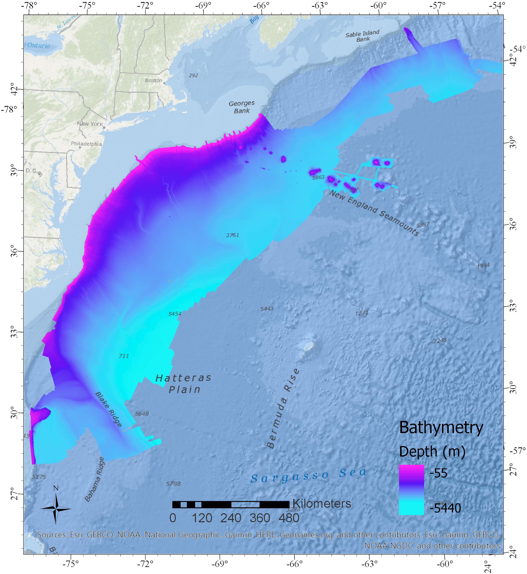
Figure 1. Bathymetric synthesis terrain model grid of the U.S. Atlantic Margin study region used as the primary data source input into the study.
Data quality was validated for the mapping cruises that generated the data used in the synthesis by the calibration of multibeam mapping systems, professional ocean mapping experts overseeing all aspects of the surveys, regular frequent sound velocity profiles of the water column, rigorous cleaning of noise and erroneous soundings following raw data collection, and cross-line validation analysis of survey areas. The synthesis of multibeam sonar data was compiled and quality controlled by an expert from the UNOLS Multibeam Advisory Committee (Johnson, 2018; Multibeam Advisory Committee, 2019). Specifics on data quality control and validation can be found in the individual publicly available cruise reports for each cruise.
Bathymetry for the deeper regions of the study area (generally deeper than 2000 m) were collected as part of the ECS Project by CCOM/JHC. Data were collected on eight different cruises between 2004 and 2015, using 12-kHz, Kongsberg EM120 or EM122 multibeam sonars. Data were acquired with the initial purpose of supporting the determination of the outer limits of the U.S. juridical continental shelf consistent with international law.
Shallower bathymetry data that cover the shelf break and Atlantic canyons out to depths of the coverage of ECS cruises were collected for the National Oceanic and Atmospheric Administration (NOAA) Atlantic Canyons Undersea Mapping Expeditions (ACUMEN) Project using NOAA vessel Okeanos Explorer. Data were collected during nine different cruises using a 30-kHz Kongsberg EM302 multibeam sonar on the Okeanos Explorer between 2011 and 2014.
Interpretation of Seafloor Landforms
The analysis of the bathymetric terrain model of the study area utilized the bathymetry- and reflectivity-based estimator for seafloor segmentation (BRESS) method developed by Masetti et al. (2018). This tool is a free stand-alone application available at https://www.hydroffice.org/bress/main (Hydroffice, 2019). The BRESS analytical approach implements principles of topographic openness and pattern recognition to identify terrain features that can be classified into easily recognizable landform types such as valleys, slopes, ridges, and flats. These “bathymorphon” architypes represent the relative landscape relationships between a single grid node and surrounding grid nodes as assessed in eight directions around the node. The position of a grid node relative to others in the terrain are determined via a line-of-sight method looking out in each direction by a user defined search annulus specified by an inner and outer search radius. Details on this approach to geomorphic terrain analysis can be found in Jasiewicz and Stepinski (2013).
An important distinction between this method and many other terrain analysis algorithms is that the identification of landform elements between a grid node and eight directions around it self-scales to adjacent features, whereas many terrain analysis algorithms work using a fixed neighborhood “moving window” approach (Jasiewicz and Stepinski, 2013). The grid neighborhood approach will identify fine features with a small cell window frame, and larger features with a bigger window, while the geomorphon approach has the capacity to capture both scales to some extent (within the limits of a defined search annulus). This is because it calculates elevation values (using both zenith and nadir angles) between the grid node and the maximum change in height of surrounding features (positive or negative) via a “line-of-sight” approach.
The bathymetry- and reflectivity-based estimator for seafloor segmentation algorithm was used to identify bathymorphon patterns in the bathymetric surface, generate area kernels (aggregations of the same bathymorphon type) and then utilizing a look-up classification table, these patterns were translated into landform types. The original geomorphon work (Jasiewicz and Stepinski, 2013) proposed a ten-type landform classification: flat, peak, ridge, shoulder, spur, slope, pit, valley, footslope, and hollow. BRESS introduced a simplified six-type landform classification (flat, ridge, shoulder, slope, valley, and footslope) and, recently, a minimalistic classification (flat, ridge, slope, and valley). The most simplistic classification was determined to be the best choice for the extremely large study area in this case, resulting in the creation of a continuous landform map of the Atlantic Margin region comprised of four classes: flat, slope, ridge, and valley.
Key user defined parameters in the landforms analysis tool within BRESS are the inner and outer radius of the search annulus and the flatness parameter. If the inner radius is set too small results can be negatively impacted by noise near the grid node (e.g., multibeam sonar surveying sound velocity offsets or outer beam “striping” artifacts in the bathymetry grid). The search annulus units are grid nodes, so the length of this is dependent directly on the resolution of the input raster grid. Alternatively, the user may specify the search radius parameters in meters. Reasonable values for the search annulus are fairly intuitive to a skilled analyst and are informed primarily by the scale of the features one is seeking to detect and the resolution of the bathymetric grid. The default parameters of inner/outer radii of 5/10 grid nodes, respectively, work well for many terrains. For this study extensive testing of the parameters on different regions of the grid revealed that an inner radius of 3 grid nodes and an outer radius of 15 grid nodes resulted in the delineation of landform features most comparable to what would be manually classified by a skilled analyst. This was determined by varying the inner and outer radius parameters of the model and draping the automatically classified landform spatial layers over the bathymetry for examination within 3D visualization software (QPS Fledermaus). The results were then evaluated to determine if delineations among landforms aligned with logical topographic feature breaks and to assess if the key morphologies of interest in the terrain (in this case ridges, slopes, valleys, and flats) were identified. Separate manual landform classification maps were not generated in this study for direct comparison with the automatic classification results, as they would be as equally subjective as the methodology used and therefore offer limited additional insights. The bathymetric grid used in this study was 100 m resolution, so the inner search radius was equal to 300 m and the outer radius was equal to 1500 m.
Results of the landforms analysis are sensitive to the choice of flatness parameter. Too large a flatness number will result in low to moderate relief seafloor features being classified as “flat,” and too small a number will result in excessive “slope” results. This parameter was tested extensively in both the steep terrains (continental canyons and seamounts) and low relief terrains (e.g., abyssal plain) found in the study region. Testing results determined that one flatness parameter could not yield useful results for the entire region. It was determined that the extremely steep seamounts needed a flatness parameter of 5.0 degrees, the continental slope region of the margin needed a flatness parameter of 3.0 degrees, and the low gradient regions of the Blake Ridge and abyssal plains needed a flatness parameter of 1.0 degree. In order to apply the necessary variable flatness terrain values to the bathymetry, a separate spatial layer mask was created using the masking tool in BRESS, then applied to compute landforms (Figure 2). This flatness angle mask spatial layer was generated manually via interpretation of the logical bathymetric breaks among the continental slope, abyss, and seamount features.
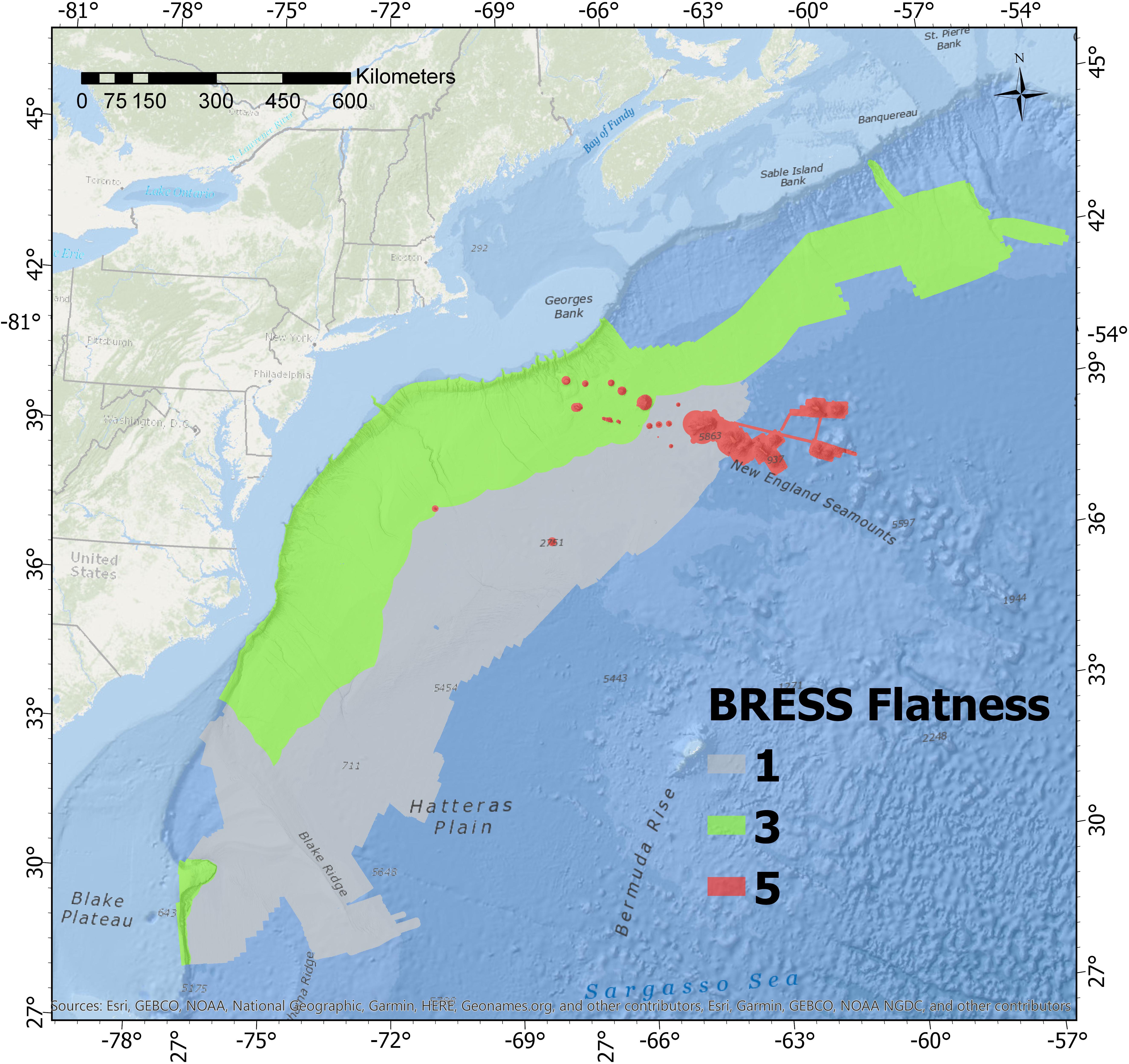
Figure 2. Flatness parameter mask used to apply different flatness values of the BRESS landform algorithm to different regions of the Atlantic Margin study area. Parameter of 5.0 degrees (red) applied to the seamounts, 3.0 degrees (green) applied to the continental slope, and 1 degrees (gray) applied to abyssal areas. Bathymetry data shown in the background for context.
The initial output of the landforms classification identified most of the prominent landform features of interest in both high and low relief areas of the study region. However, within low relief areas, a limited number of linear artifacts from the outer beam striping typical of multibeam sonar mapping systems were visible and easily discernible from real seafloor features. These small artifacts were minor and typical of the increased uncertainty of soundings in the outer beams of multibeam sonars, and were not the result of any interpolation of the original underlying dataset. Given the low flatness parameter applied to abyssal areas, the larger bumps in the outer swath sectors of multibeam in a few isolated areas were classified by BRESS as small landforms other than flats. These classification artifacts occurred in small select regions of the overall abyssal region of the grid, and were manually reclassified to flats via the application of a user-generated mask. This targeted manual quality control of the landform classification output was completed via visual inspection of the landforms draped on the bathymetric grid, and areas were corrected by encircling in a polygon using the masking tool within the BRESS software. While not an automated process, this tool provides a quick and effective quality check to improve the appearance and quantitative results of the analysis over survey areas subject to limited systematic artifacts from multibeam sonar surveys.
The output from the BRESS landform tool is either an ASCII Grid file or a geotiff image that can be imported into any spatial analysis or visualization software that can read these formats. The resolution of the output ASCII exactly matches the resolution of the input bathymetry file, in this case 100 m. The ASCII file consists of raster cells with code values that represent the landform designation of the nodes in the grid. In this case there were four code values representing each of the four landform classes derived from the lookup table in BRESS: 1 for flats, 3 for ridges, 6 for slopes, and 9 for valleys.
Conversion of Landform Units to Coastal and Marine Ecological Classification Standard Geoform Units
The landform raster output from BRESS (a grid file in ASCII Grid format) was imported into ArcGIS Pro version 3.2 for additional analysis and conversion of landform units into CMECS geoform units. Landform units were modified to delineate CMECS geoforms using decision rules based on existing CMECs standard definitions of units. CMECS provides a catalog of units for geoform classification, along with definitions of each unit class in the standard document (Federal Geographic Data Committee [FGDC], 2012). Since CMECS is intended to be a dynamic content standard, the user is able to propose “provisional units” if the existing units do not adequately meet classification needs. This study proposes one new geoform called “valley” (not to be confused with the existing CMECS term “submarine canyon” which is a specific type of valley as explained further later) and six new geoform types that are intended to describe specific types of geoforms unique to deep sea features (Table 1).
Table 1. CMECS geoform classes mapped within the Atlantic Margin study area.
Landform classes were converted to CMECS geoforms primarily by re-naming them as appropriate for the marine setting in which the units occurred throughout the extent of the Atlantic Margin. While landform units can be thought of as the primary building blocks for the identification of larger geomorphic seafloor features (e.g., canyon complexes and sand wave fields) it is proposed here that they also have value in many cases for direct translation into classified geomorphic features. This assertion is based on the fact that the landform features identified for the study area largely fit well within the existing geomorphic classification scheme being applied (CMECS). As apparent from Table 1, the landform types “flat,” “ridge,” and “slope” are also existing geoform units within CMECS. So a direct translation from landforms to geoforms for these cases was logical.
Although existing CMECS units worked well for direct translation of some landforms, other terms that are useful are not yet part of the standard. For instance, valley features were evident in all of the major study regions evaluated (continental slope, abyssal plain, and seamounts), but the concept of a valley feature in the deep sea is absent from CMECS. CMECS currently has Submarine Canyons (Physiographic Setting), Shelf Valleys (Level 1 geoform), and Channels (Level 1 and 2 geoforms). None of these classification terms are adequate descriptors for all of the valleys observed in deep sea environments. While certainly some of the valley features on the continental slope and on seamounts and guyots could be called “submarine canyons,” there are many valley features in these areas identified as valleys in the landform analysis which are not submarine canyons. Fortunately, CMECS was designed to be a dynamic content standard subject to user refinement and open to proposals for formal future modifications. Users are advised to designate “provisional units” for classes that are deemed useful but absent from the current version of the standard. Therefore, this study designated the term “valley” as a provisional geoform unit for now (column 5 in Table 1), and then defined provisional geoform type units (another step down in the classification hierarchy, column 6 in Table 1) to describe the specific types of valleys occurring within the context of different features in the deep ocean (continental slopes, abyssal areas, and seamounts).
CMECS currently lacks geoform terms that adequately describe the geomorphology of features found within seamount features. Seamounts as entire features are covered by the standard, as there is a Seamount geoform unit and both Guyot and Pinnacle Seamount geoform types defined. It is proposed that adding Guyot Flat, Seamount Ridge, Seamount Slope, and Seamount Valley would all be useful unit additions to the standard. These units are shown as provisional units in Table 1. Seamounts have been demonstrated to be hotspots of biological diversity in the deep sea. Ocean exploration ROV dives on seamounts have found that ridge features and the edges of guyots can support dense and diverse aggregations of deep sea corals and sponges, where sessile attached fauna take advantage of the combination of exposed hard substrates and food-supplying currents that can occur in these relatively rare topographic areas (see for example NOAA CAPSTONE expedition results in Raineault et al., 2018).
It is important to note that this study did not classify and map geoforms that are comprised of a complex aggregation of landforms. For instance, a submarine canyon is an important feature to map and identify along continental margins, and a CMECS geoform descriptor exists for this feature. However, a typical manual delineation encircling a complete canyon system would encompass the following separate landform types: a channel at the bottom of the valley (thalweg), the steep valley walls, and the ridges on the tops of the slopes. Therefore this single geomorphological unit is comprised of valley, slope, and ridge landforms [refer to Harris et al. (2014) for example]. Complex submarine canyon systems contain many of these features, as well as flats and more complex landforms not part of the current scheme (e.g., pits, peaks, and shoulders, etc.). Also, since the purpose of this study was to demonstrate what can be done via semi-automated terrain analysis tools over very large regions manual delineation of these more complex morphologies was not attempted.
CMECS is structured with physiographic setting high up in the hierarchy in order to discriminate between continental shelf, continental slope, abyssal plain, and seamount features. Therefore it was necessary to spatially delineate the study region into these categories. This was done by using the flatness mask ASCII grid which was already developed during landform modeling, as it was driven directly by the need to apply different flatness parameters to the continental slope, abyssal plain, and seamount regions. The mask was modified for the region offshore of Canada, as this region was mostly deep abyssal plain for the purposes of geoform classification, but was originally given the flatness parameter applied to the continental shelf due to the need to minimize classification of significant multibeam artifacts. While the term “continental rise” is a physiographic setting term in CMECS, it was not used in the study. This was because the Atlantic Margin has a gradual slope in many areas that makes it challenging to discriminate between a continental slope and a continental rise, and if present, a flattening out in gradient did not appear to occur until depths of 4000 m at the shallowest. In these settings, it was logical to refer to the area deeper than this as part of the abyssal plain. The global geomorphology classification study by Harris et al. (2014) did define a continental rise along the U.S. Atlantic continental margin, but the resolution of the data and methods for that study were different, and the results were therefore not applied to this study.
Delineation of seamounts from abyssal plain was straightforward, with clear topographic breaks between the two. The mask provides a more subjective delineation of continental slope and abyssal plain regions based on professional judgment of the approximate transition zone between the two. This was done visually based on the bathymetry grid and the approximate location of where the gradient flattened out. Using the depth contour lines was another option as a way to distinguish between continental slope and abyssal landforms, but this was not selected because it was a poor fit for the actual feature breaks along the entire length of the margin. Based on examining the changes in gradient along the margin, the demarcation mask between continental slope and abyssal areas was established generally between 4000 and 5000 m in depth along most of the margin, except for the southern region which has the dramatically different features of Blake Ridge and Blake Escarpment. Because of its character in relation to CMECS concepts, all of Blake Ridge was included in the abyssal marine basin floor category even though it gets shallower than 3000 m for a small portion in the study area. The logical topographic break on the Blake Escarpment was at the base of the escarpment at a depth contour of approximately 5000 m.
Although depths greater than 3000 m in the ocean are commonly referred to as abyssal depths, along the Atlantic Margin in many areas the actual depth where the continental slope flattens out onto an abyssal plain is substantially deeper. Alternatively, using a smoothed (generalized) gradient map of the margin was also evaluated, but was also not deemed an effective delineation approach in this case. Although the U.S. ECS Program refers to the continental slope and determines foot of the slope for juridical purposes, those delineations are a special use case unrelated to ecological processes or classification. The mask used to delineate among seamounts, continental slope, and abyssal regions for this study’s specific purpose of classifying CMECS geoforms is shown in Figure 3. This mask was created manually via expert interpretation, and was a modification of the flatness parameter mask used in BRESS software for the landforms analysis.
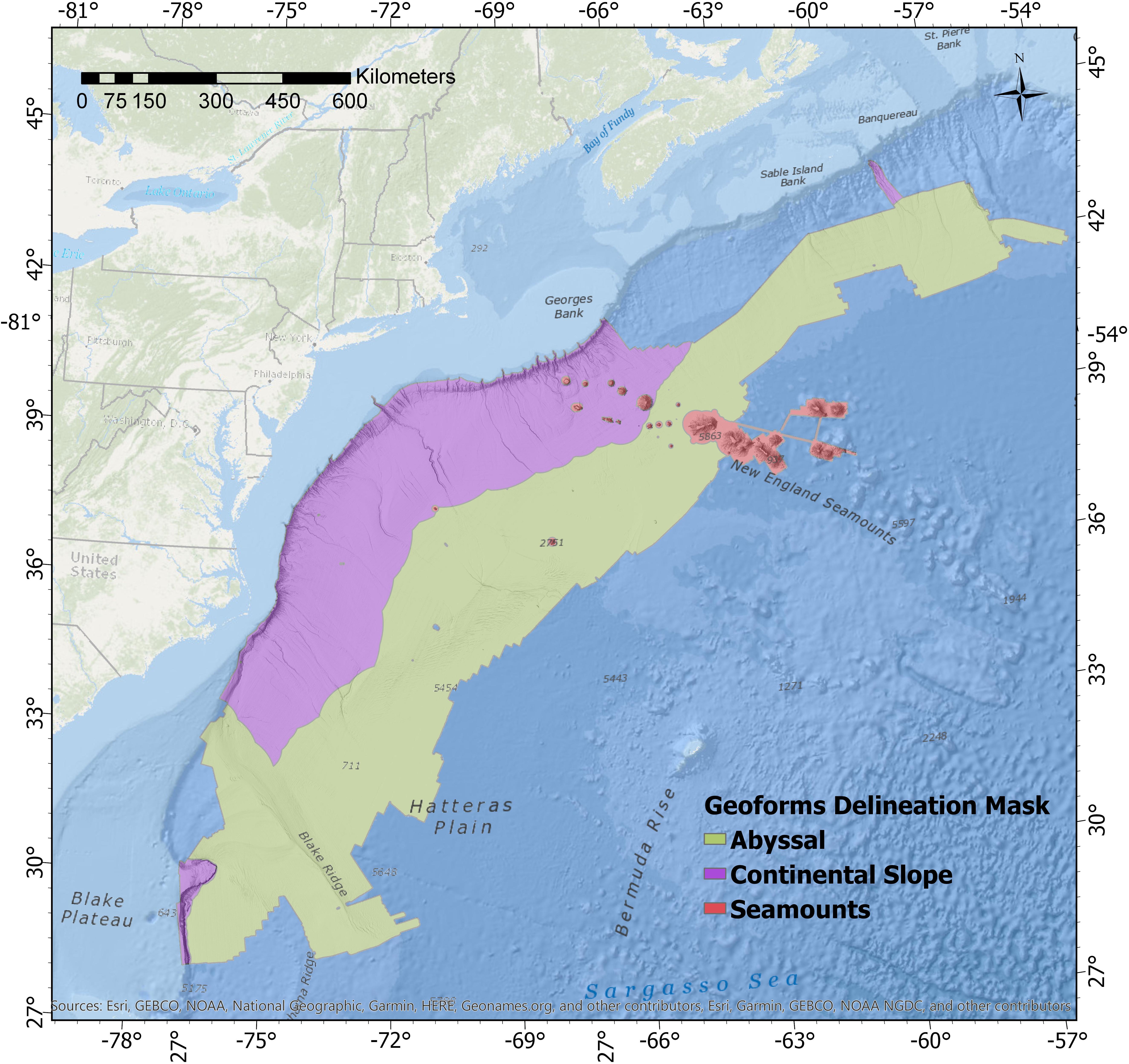
Figure 3. Regional mask applied to the study region in order to provide approximate CMECS classification boundaries between continental slope areas (purple shading) seamounts (red shading), and abyssal regions (green shading). Bathymetry data is shown in the background for context. The key difference with the Figure 2 (flatness parameter) mask is that the deep areas offshore of Canada are included with the abyssal (i.e., deep and low gradient) areas, whereas in Figure 2 that area was masked differently because it had low relief features that were hard to discriminate from multibeam mapping artifacts in the bathymetry and thus needed a larger flatness parameter value.
For visualization purposes the raster grid output of landforms from BRESS was imported into QPS Fledermaus software (version 7.7.9) and draped onto the bathymetric grid. This provided for effective three-dimensional exploration of the landform interpretation directly on top of the bathymetry from which is was derived (see Figure 4 in section “Results”). This method was utilized to evaluate the results of testing various search annulus and flatness parameter settings from the BRESS landforms tool, as well as for visualization of the final output prior to further geoprocessing in ArcGIS Pro.
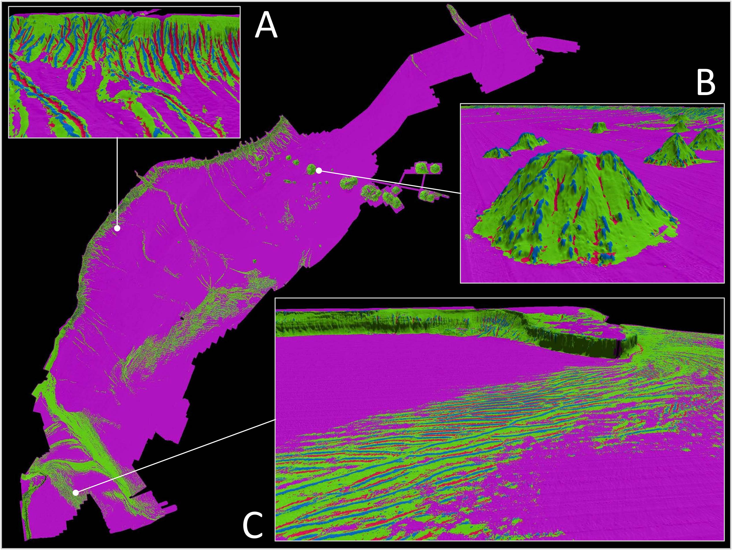
Figure 4. Continuous coverage landform map of the Atlantic Margin study region classified into four landform types: flats (purple), slopes (green), ridges (blue), and valleys (red). Oblique 3-D inset views of landform type draped on bathymetry provided to show details. Note the clear delineation of canyon ridges, valleys, and steep slopes on the continental slope (A). Seamount features are dominated by very steep slopes with occasional ridge and valley features (B). Several large regions of the abyssal plains exhibit bedform features that follow a distinct pattern of repeating crest and trough (slope and ridge landform) combinations. Bottom right inset highlights one of these bedform fields east of the prominent Blake Spur feature (C). Figure made with QPS Fledermaus software version 7.7.9. with vertical exaggeration of 4×.
Raster grids of the seafloor geoforms were converted in ArcGIS Pro to vector files for the creation of plots showing square kilometers within each geoform classification. These spatial files were also used to select polygons on the continental shelf to reclassify the geoform type as “continental shelf flats,” and to select the flat tops of some of the seamounts (guyots) to reclassify these areas to geoform type “guyot flats.” CMECS classifies guyots as a type of seamount, as the “seamount” unit is at the geoform level of the hierarchy, and “guyot” and “pinnacle seamount” are nested within this class at the geoform type level. This reclassification was done using manual selections in ArcGIS Pro software, but was limited to a small subset of the data given the small spatial extent of these geoform units relative to the size of the study region.
Results
Seafloor Geomorphology Maps: Landforms
The results of the landform analysis are shown in Figure 4, showing flats in purple, slopes in green, ridges in blue, and valleys in red. It is immediately notable (and expected) that the dominant landform class in the region is flats. The classification of flat doesn’t mean an area lacks any slope, it is classified as such in relation to the surrounding terrain and subject to the flatness parameter defined in BRESS. Slope landforms are the second-most dominant class, and together with flats show the dominant relief features of the Atlantic Margin even at the broad scale of the entire study region. Ridge and valley features provide insightful details into the structure and complexity of the continental slope canyons, abyssal bedform fields, and seamount features (see insets in Figure 4). Overall the landform results exhibit logical topographic breaks when draped over the bathymetry data, and the automated classification process from BRESS clearly works well for this purpose.
Seafloor Geomorphology Maps: Geoforms
CMECS geoform maps derived from the landform maps are shown in Figures 5–11. Results are shown separately for seamounts (Figures 5, 6), continental slope features (Figures 7, 8), and abyssal features (Figure 9). For each of these regions the area of each geoform unit class, and percent contribution of each class to the whole area, were calculated. Area is report in square kilometers. The relative dominance or rarity of geoform types has ramifications for the potential habitat role of these areas, and can inform management decisions pertaining to regional marine spatial planning.
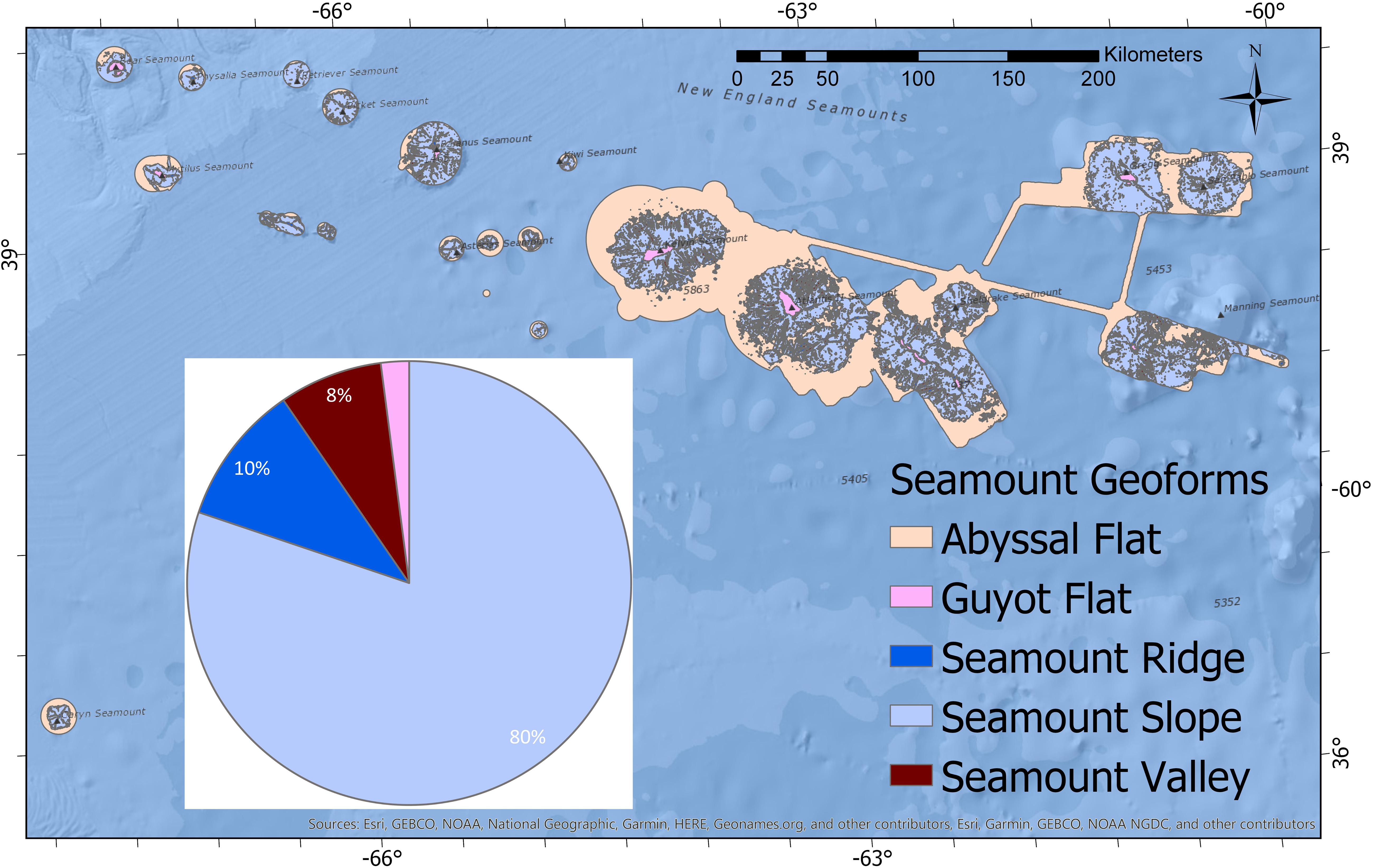
Figure 5. CMECS geoform classifications specific to seamounts. The tan area shown in the figure met the definition of the “abyssal flat” class and was added to that class for calculating overall study region summary statistics and for the map shown in Figure 11 of all geoform classes for the whole region.
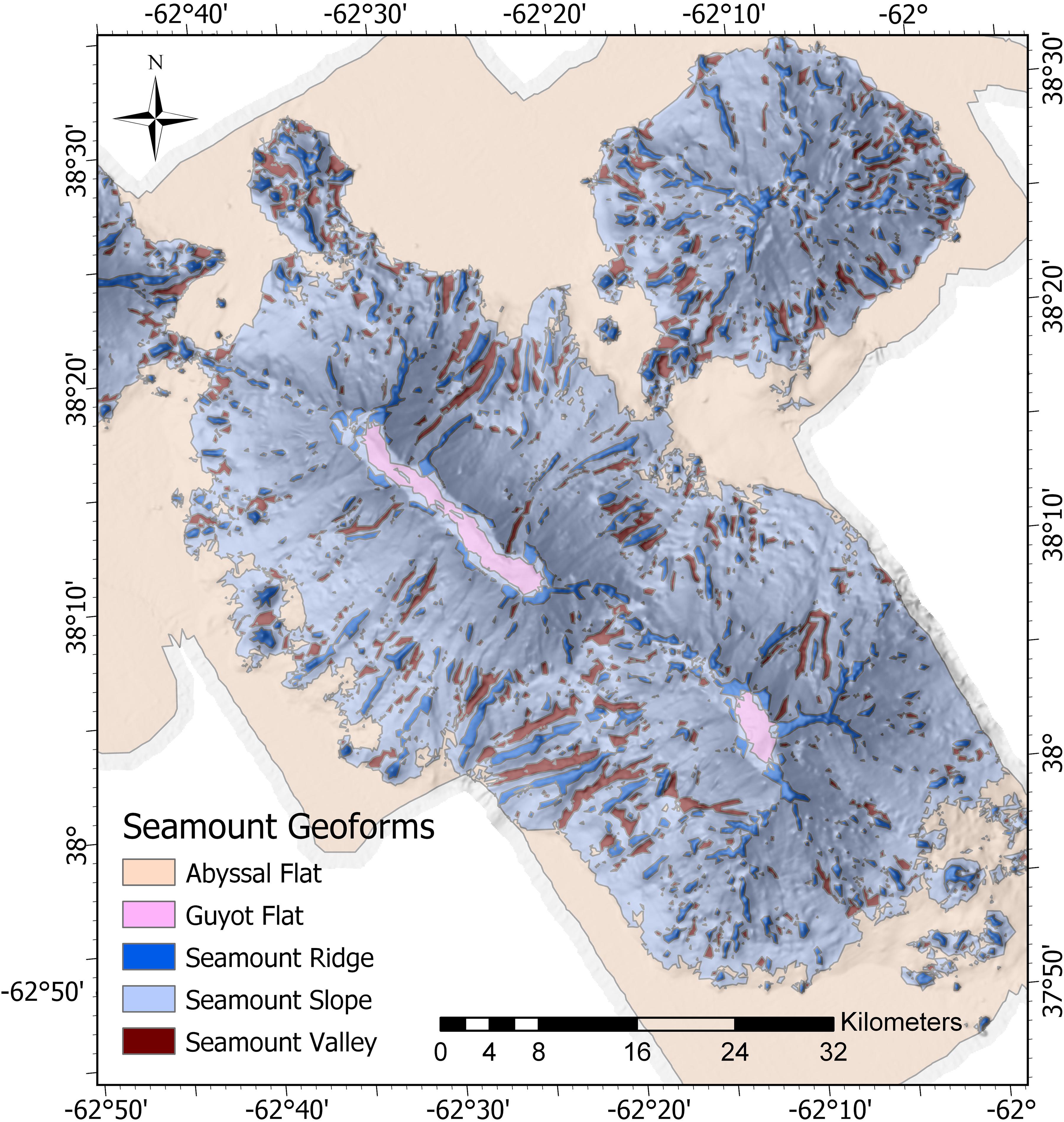
Figure 6. Geoform classes of Gosnold Seamount. A hillshade layer was computed from the bathymetry and is shown with partial transparency to provide depth and context to the figure.
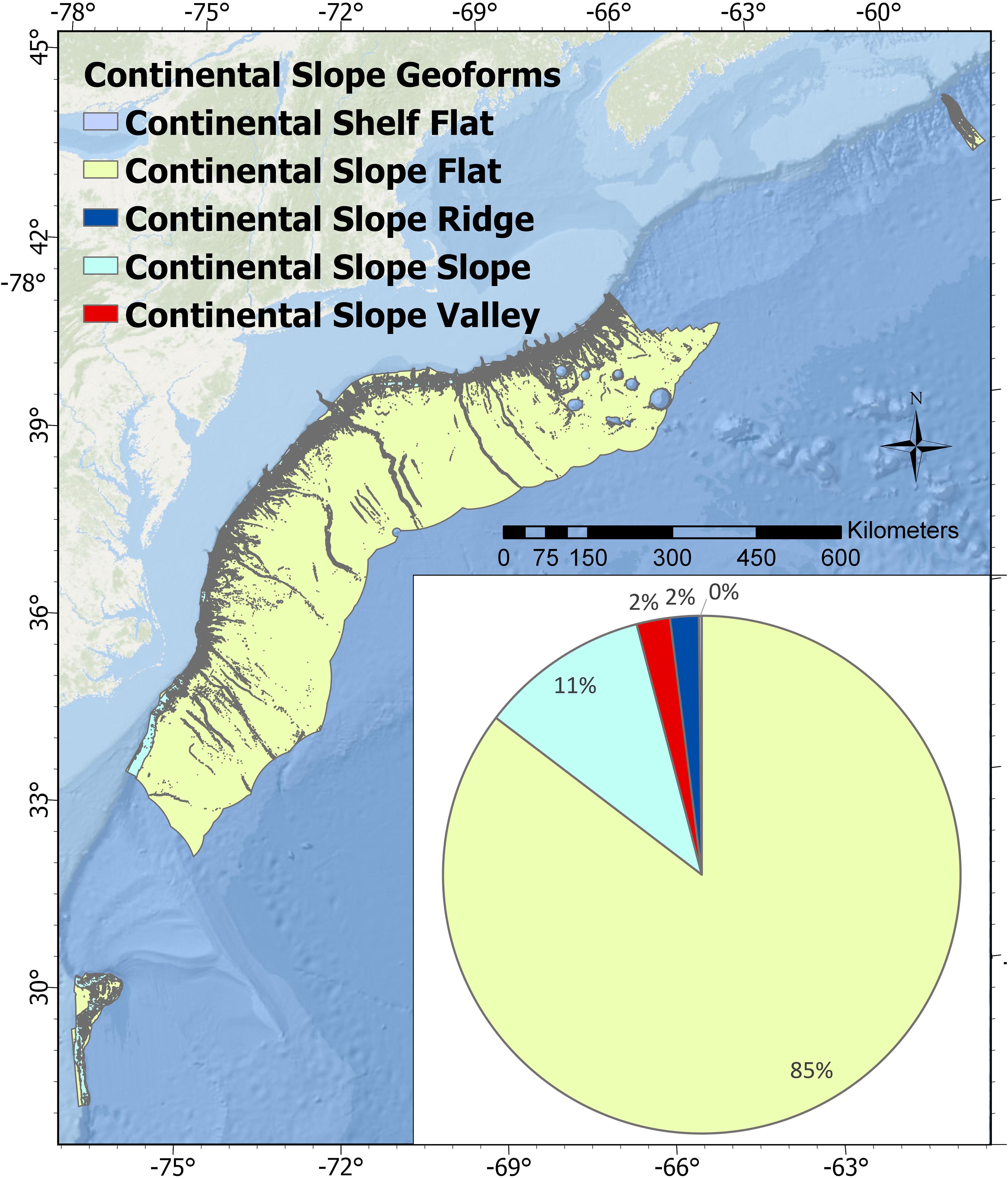
Figure 7. CMECS geoform classifications specific to the continental slope region of the study area. 85% of the area is classified as flats, followed by 11% slopes. Ridges and valleys both comprised 2% each. A very small portion of the mapped area in the study (0.2%) was classified as continental shelf flat (in the shallow areas above the heads of the canyons). These results highlight the fact the continental slope drops off dramatically within a relatively short distance down the steep Atlantic canyons region of the margin, then exhibits a mild gradient down to abyssal depths. While the “continental slope flat” geoform type (yellow green) occurs on the continental slope, it is classified as a flat relative to the steepness of the canyons region, and due to the fact that slopes in these areas are nearly uniformly gradual and tend to range from about 0.1–1.5 degrees.
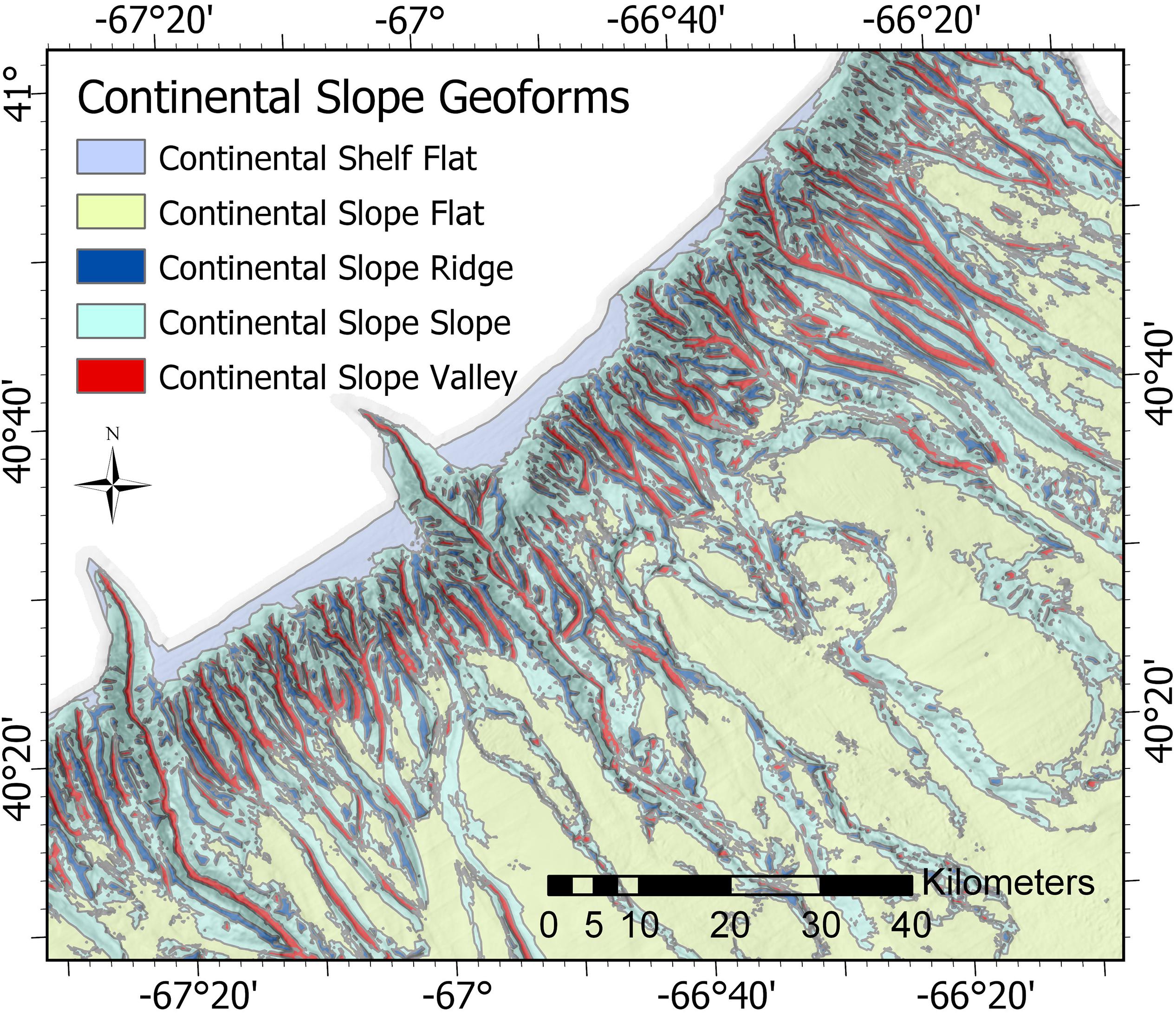
Figure 8. Prominent submarine canyon features on the continental slope in the Mid-Atlantic as classified by CMECS geoforms. This geoform map clearly highlights the extensive network of gullies and submarine canyons that are a signature feature of the region. A hillshade layer was computed from the bathymetry and is shown with partial transparency to provide depth and context to the figure.
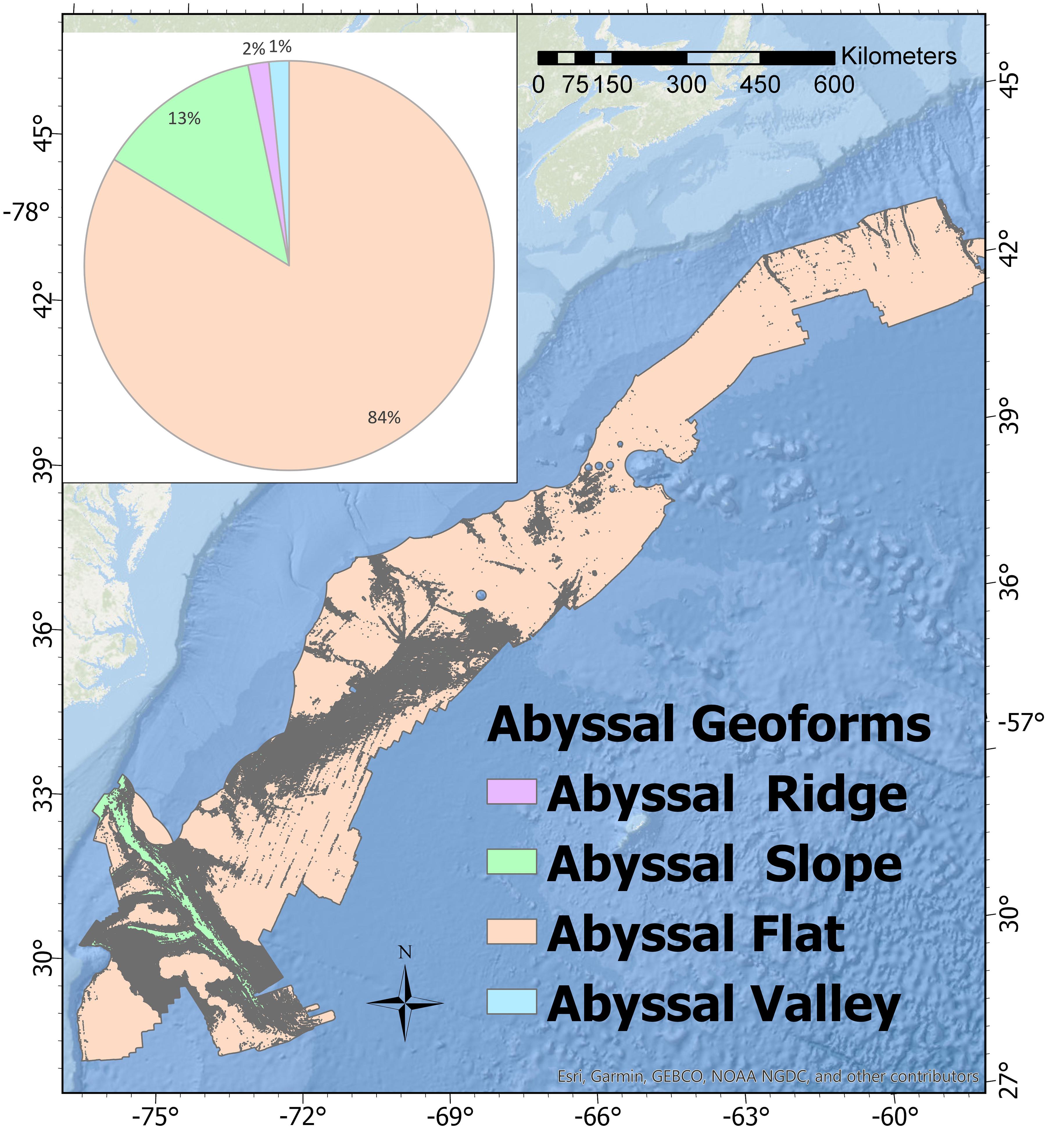
Figure 9. CMECS geoform classifications for the abyssal region of the Atlantic Margin.
Seamount geoforms are dominated by seamount slopes (80% by area). The second most notable features are seamount ridges (10%), followed by seamount valleys (8%). The uniform steepness of the seamounts on all sides and scarcity of consistent prominent ridge features as visible from the maps is consistent with these numbers. The rarity of the guyot flat class (2%) highlights how small these features truly are by area, even though their visual interest in bathymetric maps immediately makes an impression on the interpreter. Only 9 out of the 28 seamounts within the study region have flats at their tops (guyot flats).
In the abyssal region 84% of the area is classified as flats, 13% as slopes, 2% as ridges, and about 1% as valleys. Notable geoform characteristics of this region include the dominance of flats, the major contribution of the Blake Ridge feature to the slope class, and the importance of the bedform sediment wave formations in the U.S. Mid- and South-Atlantic regions to the slope, ridge, and valley classes. Bedform features and broad shallow submarine channels offshore of the Canadian margin do exist, but were not picked up by the methods used in this study given their smaller extent and vertical relief.
Figure 10 shows a complex region of the study area encompassing portions of Blake Escarpment, Blake Spur, and Blake Ridge. The figure provides mapped geoforms in both the continental shelf and abyssal portions of the study area. The bedform features in the right corner of the figure are striking, with crest-to-crest distances between about 2000–3000 meters.
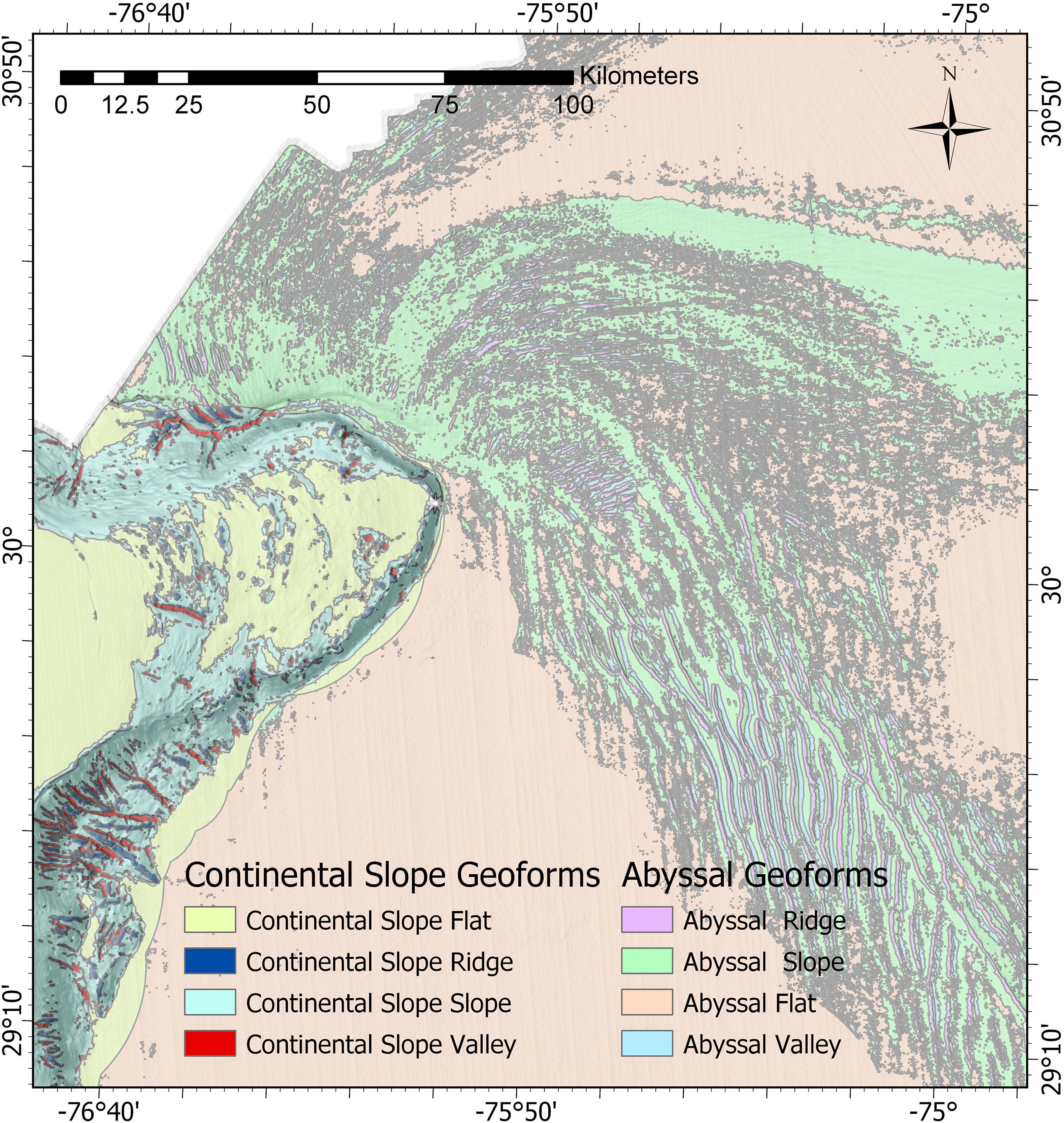
Figure 10. Geoform view of part of the Blake Escarpment and Blake Ridge.
Figure 11 illustrates the results for all geoform classes across the entire Atlantic Margin study area. Abyssal flats make up more than half of the area (53%), with the continental slope flat class making up another 30% of the total area. Flats of any geoform class (including continental shelf flats and guyot flats) make up 83.06% of the study area. Slope classes make up a cumulative total of 13.26% of the study region (8.27% abyssal slopes, 3.73% continental slopes, and 1.25% seamount slopes). While ridge features comprise only 1.82% of the total study area (1.03% abyssal ridges, 0.63 continental slope ridge, and 0.16% seamount ridges). The area (in square kilometers) and percentage calculations for each geoform class are shown in Table 2.
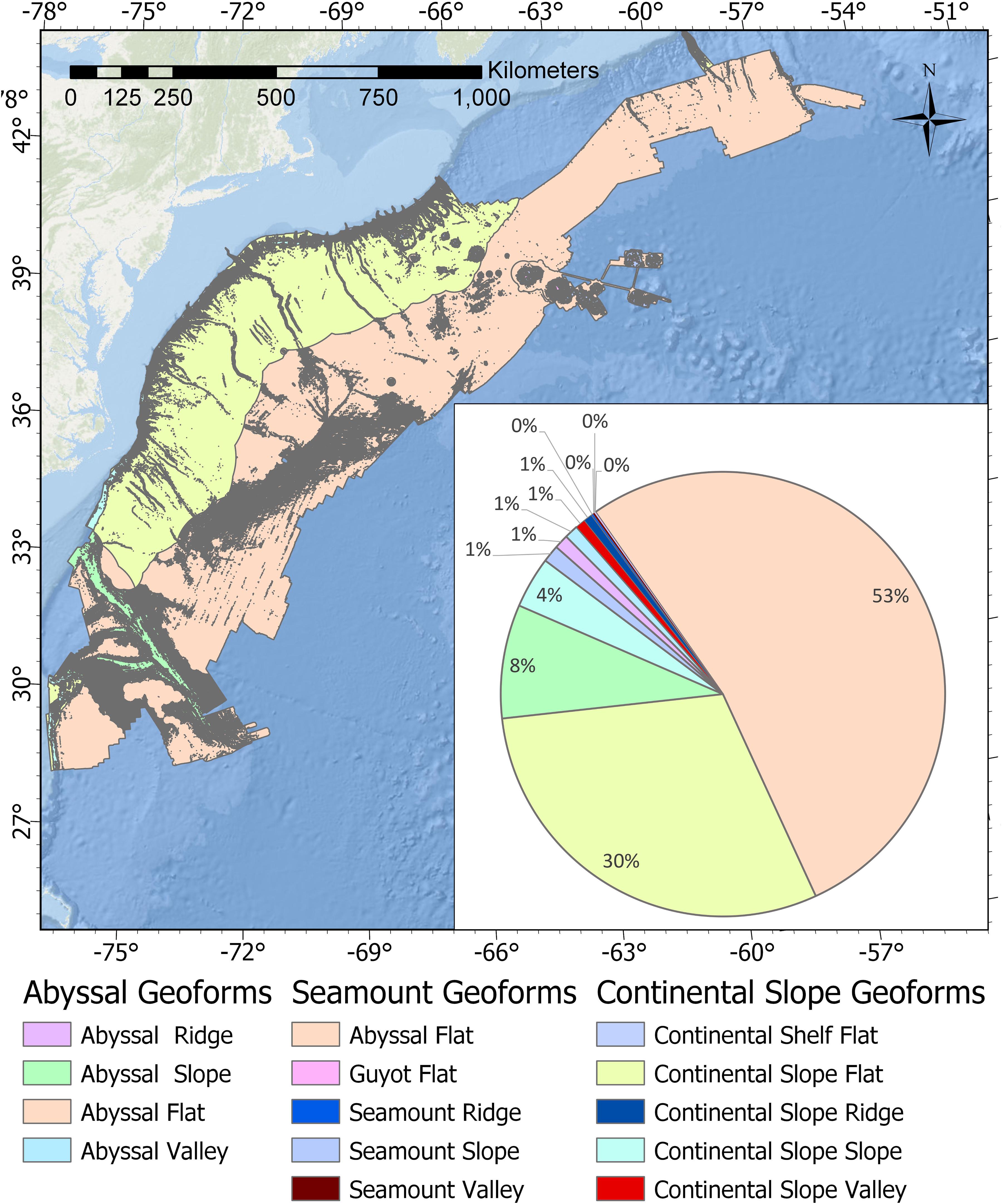
Figure 11. CMECS geoform classifications for the entire Atlantic Margin region in the study.
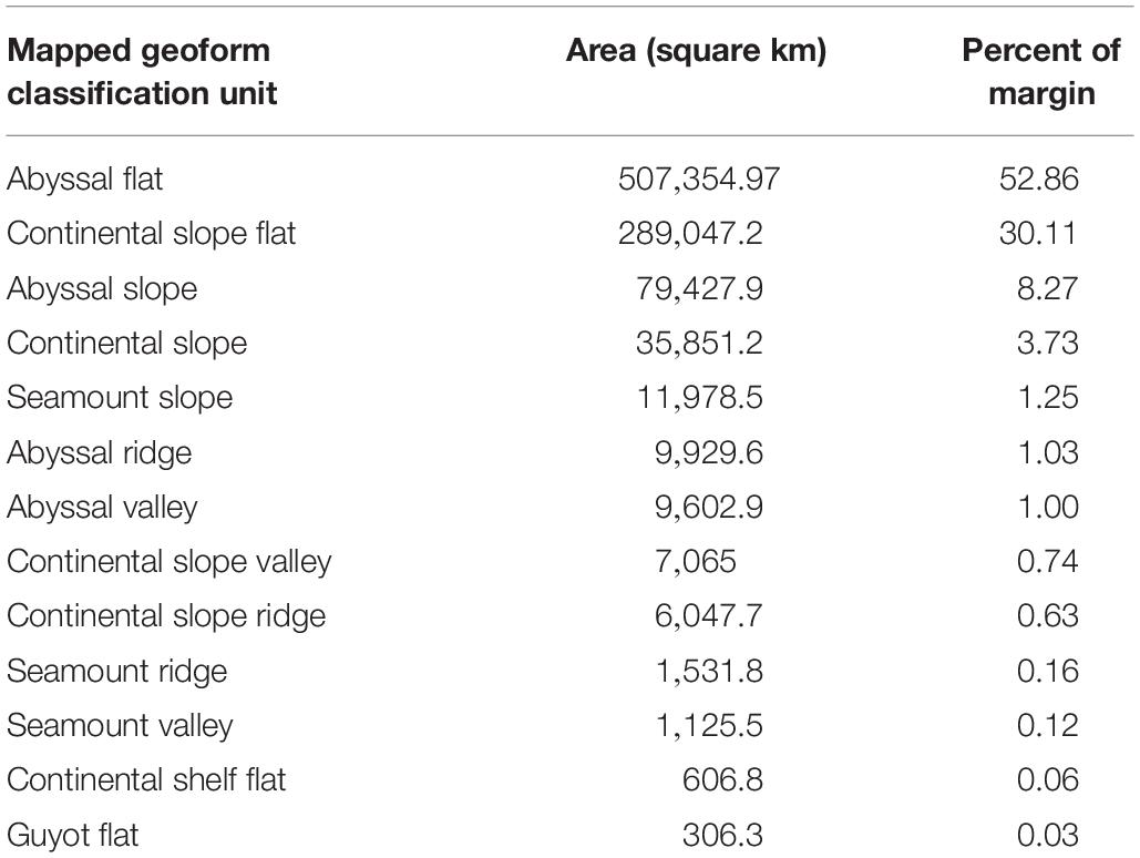
Table 2. Geoform classes of the Atlantic Margin study region by area and percentage.
Discussion
Advantages of the Semi-Automated Standardized Geomorphic Classification
This study tested the application of semi-automated terrain analysis methods and a standardized geomorphic classification scheme to a diverse region of the deep sea. The BRESS terrain analysis algorithm was effective at generating meaningful landform maps that could be readily translated to existing and proposed CMECS geoform units. Benefits of the tested methods include the following:
• The generation of landform results is repeatable and documented. The BRESS tool is based on a published mathematical terrain modeling approach, and is therefore not a “black box” tool. While improvements and refinements can be made to the algorithm, the methods are transparent.
• The semi-automated approach provides high speed classification of terrain over very large areas and complex terrain. The study area encompassed 959,875 km2. The classification work presented in this paper represents several months of focused full time analytical effort (not including initial pilot studies, refinement of study analysis methods, and improvements to software interfaces). Full coverage manual interpretation of landforms and geoforms by a skilled analyst to a comparable level of detail is estimated to take 3–5× longer.
• The classification of landforms using the study methods involve far less subjectivity than classification methods conducted manually via expert interpretation.
• The line-of-sight analytical approach to terrain analysis employed in BRESS provides benefits in its ability to self-scale to features in the terrain as versus fixed neighborhood moving window algorithms.
• The methods are adaptable to data collected with different sensors and resolutions. The BRESS landform analysis tool can utilize bathymetry data independent of the technology used to generate the data. CMECS is also designed to be data agnostic. Both of these tools can be utilized to perform similar processing workflows that remain useful with emerging seafloor mapping technology and higher resolution maps.
• The methods are scalable to very large ocean regions, making them promising tools for interpreting data collected at regional scales and in international waters.
• Due to standardized processing methods and terminology this approach can enable integration of data sets from a variety of sources and provide outputs useable across a variety of ocean governance boundaries.
Limitations of the Approach
This approach is subject to limitations typical for studies employing methods to describe and map marine habitat, including the fact that all interpretation of remotely sensed information about the marine environment is constrained by issues of spatial and temporal scale and resolution of measurement data. This study was effective at classifying broad scale features discernible from a 100m resolution bathymetric grid generated from full coverage multibeam sonar data. Smaller geomorphic pattern detection is always limited by resolution and scale considerations. The BRESS tool used in this study currently requires several trial-and-error cycles to get the parameters fine-tuned to the study area. In addition, manually generated mask spatial layers based on subjective expert interpretation were still needed to adjust the flatness parameter across the terrain, to generally delineate among continental slope, abyss, and seamount regions, and to quality control a small subset of the landform classification output. The current study is one of several other applications of the landform modeling tool aimed at improving use guidelines and best practices.
As described in the methods section, the analysis results are fairly sensitive to the selection of an appropriate flatness angle parameter. Common artifacts in multibeam mapping data result from greater uncertainty in the seafloor bottom detections of the outer beams even for fully calibrated systems with regular sound velocity measurements being taken while surveying. In several thousand meters of water depth these striping artifacts in the mapping swath can result in bathymetric grid artifacts that can partially mask seafloor features of interest. In this setting, choosing a low flatness angle in BRESS can classify low relief features like the channels shown in Figure 12. However, that is often at the expense of also classifying the striping artifacts that are also embedded into the bathymetric grid (which are not real geomorphic features). In this case, choosing a higher value for the flatness parameter ignores the classification of undesired artifacts, but also loses the ability to classify features of interest like the abyssal channels in Figure 12. This area was ultimately assigned a higher flatness parameter of 3.0 degrees in the BRESS tool in order to avoid identifying the multibeam striping artifacts as landform features.
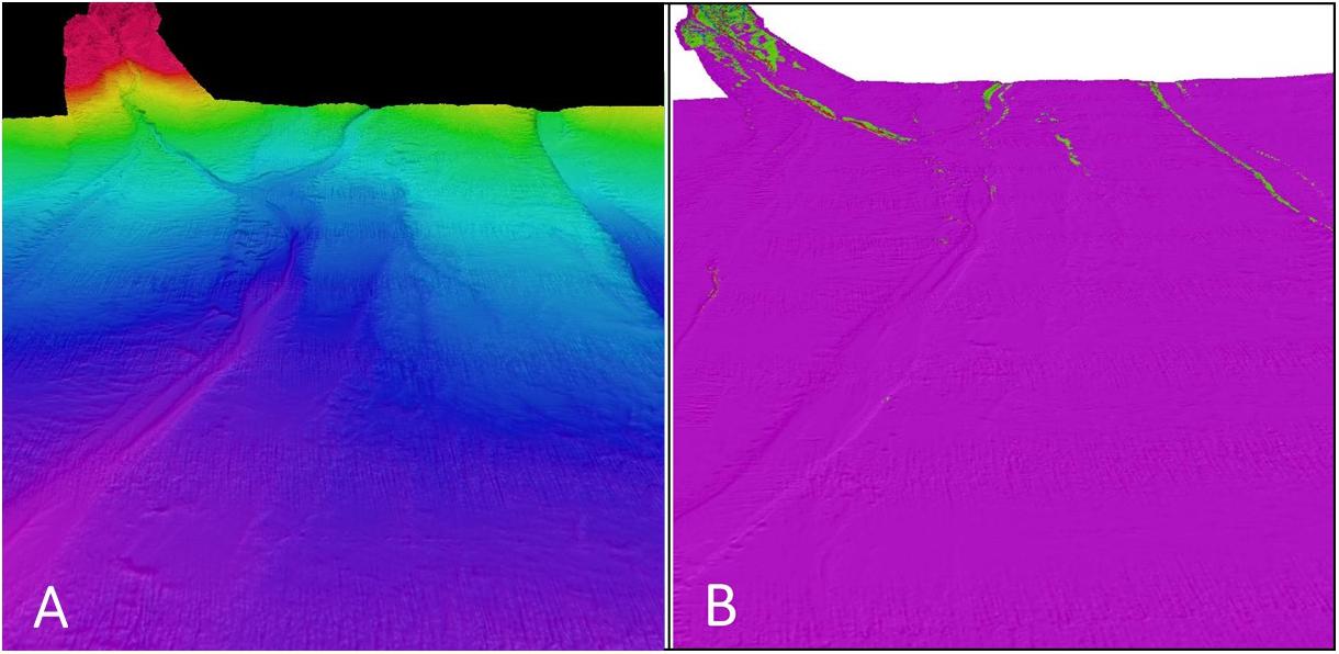
Figure 12. Perspective view comparison of bathymetry data (A) with the classified landform results as draped on bathymetry (B). Note the presence of channel features in the bathymetry that could not be resolved as geoforms using the landform parameters applied (they were classified as flats as represented by the purple color).
Complex combinations of landform elements that together aggregate into larger geomorphic features of interest were not identified in this study. A good example is the bedform features found in the abyssal plains of the study area. While the study effectively classified the slope, ridge, and valley combinations that comprise the components of larger geoforms such as a “sediment wave field,” the ability to automatically classify these aggregate geoforms is the subject of future research.
Potential Applications of Coastal and Marine Ecological Classification Standard Geomorphic Maps
Coastal and Marine Ecological Classification Standard geoform maps for the Atlantic Margin provide insights useful for informing additional characterization of the region, and for informing current management decisions. The clear delineation of channels (i.e., the red continental slope valley features shown in Figure 8) for the Atlantic canyons makes it easy to see the low points and gain insights into the potential pathways of sediment transport out onto the abyssal basins. Their delineation from the surrounding terrain makes it easy to identify and enumerate the number of distinct canyon channels and continental shelf gullies more easily than by examining the bathymetry directly. This facilitates a better assessment of the nature and number of gully and submarine canyon features on this margin, and provides a quantitative methodical basis by which to compare these attributes to the same type of features on other continental margins. Similarly, the ability to automatically delineate significant ridge features within canyons has implications for assessing the habitat associations of organisms that may utilize these features.
The relative rarity of steep slopes (i.e., >3 degree angle from surrounding terrain) and ridges in the continental slope (11 and 2%, respectively) is striking. These areas have proven to be some of the highest likelihood places capable of supporting deep sea coral and sponge communities that often attach to steep exposed hard surfaces (Quattrini et al., 2015). The canyons area is clearly a hotspot of geodiversity, and has been recognized as a hotspot for biological diversity as well. The delineation of the canyon systems into flat, slope, ridge, and valley geoforms enables simple calculations of the relative number and area of these features within a given area of interest. This type of quantitative data on marine seascapes supports more informed marine resource management decisions, including strategic planning of marine protected area designations.
The extreme rarity of the guyot flat class (0.03% of the total area of the study region) make them a potentially vulnerable habitat. Extractive fishing pressure (Clark, 2010), seafloor mining activities (Miller et al., 2018), and potential impacts from climate change (Levin, 2019) could impact these relatively small areas in different ways than more abundant geoforms and a precautionary approach to management is appropriate given their relative scarcity in the marine environment. Limited exploration of seamounts to date has revealed that many of these features also serve as hotspots of biological diversity and habitat for deep sea coral and sponge communities (Lamplugh et al., 2013).
The ability to quickly automatically classify features such as steep slopes and ridges, generate accurate spatial datasets of these features, and calculate the area encompassed within them, should be of great interest to marine predictive habitat modelers. While depth (bathymetry) is a common variable in habitat suitability modeling, having spatial layers of geoforms that are known to be strongly correlated with the presence of certain species or communities of biotic importance could support more powerful and accurate predictive models (e.g., Savini et al., 2014).
Conclusion
Our results provide a characterization of the marine landscape that serves as an inventory of the cumulative area and abundance of geoforms and the spatial relationships among them. The derived maps and associated databases can be used for a broad range of spatial analyses defined by other end users to inform management decisions. Geoform summary statistics were calculated over the study region to quantify the area of each geoform type. These analyses represent a first step in identifying regions of consistent morphology within which the consistency of the backscatter can then be determined (Masetti et al., 2018).
The approach developed through this work provides a model of how to consistently classify ecological marine units using CMECS as an organizing framework across large continental margin regions nationally or globally. Given that many nations have already invested heavily in gathering bathymetric data for these areas, this approach can be adopted to obtain a standardized interpretation to inform baseline marine habitat characterization in support of ecosystem-based management.
Data Availability Statement
The datasets generated supporting the conclusions of this article will be made available by the authors, without undue reservation, to any qualified researcher. The primary input bathymetry dataset used by this study is publicly available and located at the following website URL: https://maps.ccom.unh.edu/portal/apps/webappviewer/index.html?id=375a12ced0e242bbbb83958069bbae2d. Source datasets for each cruise that were used as part of the synthesis grid are accessible at https://maps.ngdc.noaa.gov/viewers/bathymetry/.
Author Contributions
DS and LM developed the conceptual ideas for the study as part of a larger investigation into utilizing data from the ECS Program for marine habitat characterization. DS completed the analysis of geomorphology and translation to proposed geoforms within the CMECS framework. GM created and refined the BRESS software utilized for automated identification of geomorphic landforms, and contributed substantially to the analysis and interpretation of the data. JG was Chief Scientist on 5 of the ECS cruises and processed and gridded all of the Atlantic ECS data. PJ analyzed and synthesized the regional bathymetric terrain model used as the primary data source for the study. DS, LM, and AA provided the critical revisions of the manuscript with respect to relevance to the field of seafloor characterization and ocean exploration.
Funding
Support for this research was provided by the NOAA grant NA15NOS4000200, Principal Investigator LM.
Conflict of Interest
The authors declare that the research was conducted in the absence of any commercial or financial relationships that could be construed as a potential conflict of interest.
Acknowledgments
The authors wish to acknowledge the contribution of the following collaborators to this study. Dr. Larry Ward for discussions and refinement of ideas on refining the BRESS software tool and converting landform classes to geoforms, JG for conceptualization of value-added uses for ECS datasets and leadership completing bathymetric surveys of the study area, Mark Finkbeiner for expert advice and guidance on the application of CMECS and development of this dynamic content standard, and the captains and crews of all of the oceanographic vessels involved in gathering the bathymetric data for the study.
References
Althaus, F., Williams, A., Kloser, R. J., Seiler, J., and Bax, N. J. (2012). “Evaluating geomorphic features as surrogates for benthic biodiversity on australia’s western continental margin,” in Mapping the Seafloor for Habitat Characterization, eds B. J. Todd and H. G. Greene, (Canada: Geological Association of Canada), 665–679. doi: 10.1016/b978-0-12-385140-6.00048-7
Armstrong, A. A., Calder, B. R., Smith, S. M., and Gardner, J. V. (2012). U.S. Law of the Sea Cruise to Map the Foot of the Slope of the Northeast U.S. Atlantic Continental Margin: Leg 7. Durham, NH: University of New Hampshire.
Becker, J. J., Sandwell, D. T., Smith, W. H. F., Braud, J., Binder, B., Depner, J., et al. (2009). Global bathymetry and elevation data at 30 arc seconds resolution: SRTM30_PLUS. Mar. Geodesy 32, 355–371. doi: 10.1080/01490410903297766
Brothers, D. S., ten Brink, U. S., Andrews, B. D., and Chaytor, J. D. (2013a). Geomorphic characterization of the U.S Atlantic continental margin. Mar. Geol. 338, 46–53.
Brothers, D. S., ten Brink, U. S., Andrews, B. D., Chaytor, J. D., and Twichell, D. C. (2013b). Geomorphic process fingerprints in submarine canyons. Mar. Geol. 337, 53–66. doi: 10.1016/j.margeo.2013.01.005
Calder, B. R. (2015). U.S. Law of the Sea Cruise to Map the Foot of the Slope of the Northeast U.S. Atlantic Continental Margin: Leg 8. Durham, NH: University of New Hampshire.
Calder, B. R., and Gardner, J. V. (2008). U.S. Law of the Sea Cruise to Map the Foot of the Slope of the Northeast U.S. Atlantic Continental Margin: Leg 6. Durham, NH: University of New Hampshire.
Cartwright, D., and Gardner, J. V. (2005). U.S. Law of the Sea Cruise to Map the Foot of the Slope and 2500-m Isobath of the Northeast U.S. Atlantic Continental Margin: Legs 4 and 5. Durham, NH: University of New Hampshire.
Eakins, B. W., Bohan, M. L., Armstrong, A. A., Westington, M., Jencks, J., Lim, E., et al. (2015). NOAA’s role in defining the U.S. Extended Continental Shelf. Mar. Technol. Soc. J. 49, 204–210. doi: 10.4031/MTSJ.49.2.17
European Environment Agency [EEA] (2004). European Nature Information System (EUNIS). Copenhagen, DK: European Environment Agency.
Federal Geographic Data Committee [FGDC] (2012). FGDC-STD-018-2012. Coastal and Marine Ecological Classification Standard. Reston, VA: Federal Geographic Data Committee.
Gardner, J. V. (2004). U.S. Law of the Sea Cruise to Map the Foot of the Slope and 2500-m Isobath of the Northeast U.S. Atlantic Continental Margin: Cruises HO4-1,2, and 3. Durham, NH: Center for Coastal and Ocean Mapping/Joint Hydrographic Center.
Harris, P. T. (2012a). “Biogeography, benthic ecology and habitat classification schemes,” in Seafloor Geomorphology as Benthic Habitat: GeoHab Atlas of Seafloor Geomorphic Features and Benthic Habitats, eds P. T. Harris and E. K. Baker (Amsterdam: Elsevier), 61–91. doi: 10.1016/b978-0-12-385140-6.00004-9
Harris, P. T. (2012b). From Seafloor Geomorphology to Predictive Habitat Mapping: Progress in Applications of Biophysical Data to Ocean Management. Canberra: Geoscience Australia.
Harris, P. T., and Baker, E. K. (eds) (2011). Seafloor Geomorphology as Benthic Habitat: GeoHab Atlas of Seafloor Geomorphic Features and Benthic Habitats. Amsterdam: Elsevier.
Harris, P. T., MacMillan-Lawler, M., Rupp, J., and Baker, E. K. (2014). Geomorphology of the oceans. Mar. Geol. 352, 4–24. doi: 10.1016/j.margeo.2014.01.011
Hydroffice (2019). Bathymetric- and Reflectivity-Based Estimator of Seafloor Segments (BRESS). Available at: https://www.hydroffice.org/bress/main (accessed May 6, 2019).
Jasiewicz, J., and Stepinski, T. F. (2013). Geomorphons - A pattern recognition approach to classification and mapping of landforms. Geomorphology 182, 147–156. doi: 10.1016/j.geomorph.2012.11.005
Johnson, P. (2018). Atlantic Margin Bathymetry and Backscatter Map Viewer. Available at: https://maps.ccom.unh.edu/portal/apps/webappviewer/index.html?id=b130c6b32d9d4273af0ae1733ce19905 (accessed June 15, 2019).
Kennedy, B. R. C., Cantwell, K., Malik, M., Kelley, C., Potter, J., Elliott, K., et al. (2019). The unknown and the unexplored: insights into the Pacific Deep-Sea following NOAA CAPSTONE expeditions. Front. Mar. Sci. 6:480. doi: 10.3389/fmars.2019.00480
Lamplugh, M., Forbes, S., and Armstrong, A. A. (2013). Joint Canada -U.S. Mapping Cruise in Support of Extending Territorial Claim Under the United Nations Convention on the Law of the Sea: Canadian Scotian Shelf. Final Field Report #2600352. Ottawa: Canadian Hydrographic Service.
Levin, L. A. (2019). Sustainability in deep water: the challenges of climate change, human pressures, and biodiversity conservation. Oceanography 32, 170–180. doi: 10.1002/2017WR020970
Lobecker, E. (2019a). Mapping Data Acquisition and Processing Summary Report: Cruise EX-12-04 Exploration: Northeast Canyon and Continental Margins Mapping (Mapping). Silver Spring, MD: NOAA. doi: 10.5670/oceanog.2019.224
Lobecker, E. (2019b). Mapping Data Acquisition and Processing Summary Report: Cruise EX-13-03, New England Seamount Chain Exploration (Mapping). Silver Spring, MD: NOAA.
Lobecker, E. (2019c). Mapping Data Acquisition and Processing Summary Report: Cruise EX-13-04 Leg 2 Northeast United States Canyons Exploration. Silver Spring, MD: NOAA.
Lobecker, E., Cantelas, F., Skarke, A., Peters, C., Stuart, L., Harris, A., et al. (2011). Mapping Data Report: Cruise EX-11-06 Exploration Mapping, Pascagoula, Mississippi to Davisville, Rhode Island. Silver Spring, MD: NOAA.
Lobecker, E., Doroba, J., Pinero, C., Smithee, T., Kok, T., Kennedy, B., et al. (2017a). Mapping data acquisition and processing report, cruise EX1202 Leg 2: Exploration: Gulf of Mexico, March 19 - April 7, 2012 Tampa, FL to Pascagoula, MS. Silver Spring, MD: NOAA.
Lobecker, E., Elliott, K., Gallant, L., James, J., Conway, R., and Raymond, A. (2015a). Mapping Data Acquisition and Processing Report, Cruise EX-13-04 Leg 1, Exploration, NE Canyons, July 8 - 25, 2013. Silver Spring, MD: NOAA.
Lobecker, E., Gray, L. M., and Skarke, A. (2019). Mapping Data Acquisition and Processing Summary Report: Cruise EX-12-06 Northeast and Mid-Atlantic Canyons Exploration (Mapping). Silver Spring, MD: NOAA.
Lobecker, E., and Malik, M. (2019a). Mapping Data Acquisition and Processing Summary Report: Cruise EX-12-01 Ship Shakedown and Patch Test Canyons and Continental Margin Exploration (Mapping). Silver Spring, MD: NOAA.
Lobecker, E., and Malik, M. (2019b). Mapping Data Acquisition and Processing Summary Report: Cruise EX-12-05 Leg 2 Canyons and Continental Margin Exploration (Mapping). Silver Spring, MD: NOAA.
Lobecker, E., and Sowers, D. (2019). Mapping Data Acquisition and Processing Summary Report: Cruise EX-14-01 Mission Systems Shakedown and Patch Test (Mapping). Silver Spring, MD: NOAA.
Lobecker, E., Malik, M., Gallant, L., Stuart, L., James, J., Conway, R., et al. (2015b). Mapping Data Acquisition and Processing Report, Cruise EX-13-02 : Ship Shakedown & Multibeam Patch Test, ROV Shakedown & Field Trials, NE Canyons Exploration, May 13 - June 6, 2013, Charleston, South Carolina to North Kingstown, Rhode Island. Silver Spring, MD: NOAA.
Lobecker, E., Malik, M., Gallant, L., Stuart, L., James, J., Nadeau, R., et al. (2014). Mapping Data Acquisition and Processing Report, Cruise EX-13-01: Ship Shakedown & Patch Test & Exploration, Northeast Canyons (Mapping), March 28 - April 5, 2013 N. Kingston, RI - N. Kingston, RI. Silver Spring, MD: NOAA.
Lobecker, E., Skarke, A., Nadeau, M., Brothers, L., Bingham, B., Stuart, L., et al. (2012). Mapping Data Acquisition and Processing Report : Cruise EX1205 Leg 1, Exploration Blake Plateau, July 5 - 24, 2012. Silver Spring, MD: NOAA.
Lobecker, E., Sowers, D., McKenna, L., Rose, E., James, J., Weller, E., et al. (2017b). Mapping Data Acquisition and Processing Report, Cruise EX-14-02 Leg 1: Mission System Shakedown and Patch Test, February 24 - March 15, 2014 N. Kingstown, RI - N. Kingstown, RI. Silver Spring, MD: NOAA.
Malik, M., Stuart, L., Argento, A., Denney, S., Flinders, A., Whitesell, D., et al. (2012). Mapping Data Report. Cruise EX1203, Exploration Mapping, Gulf of Mexico, May 5 - May 23, 2012, Galveston, TX to Norfolk, VA. Silver Spring, MD: NOAA.
Masetti, G., Mayer, L. A., and Ward, L. G. (2018). A bathymetry- and reflectivity-based approach for seafloor segmentation. Geosciences 8:14. doi: 10.3390/geosciences8010014
Mayer, L., Jakobsson, M., Allen, G., Dorschel, B., Falconer, R., Ferrini, V., et al. (2018). The Nippon Foundation - GEBCO seabed 2030 project: the quest to see the World’s Oceans Completely Mapped by 2030. Geosciences 8:63. doi: 10.3390/geosciences8020063
McKenna, L., and Kennedy, B. (2015). Mapping Data Acquisition and Processing Report, Cruise EX-14-04 Leg III : Exploring Atlantic Canyons and Seamounts (ROV and Mapping), September 16 to October 7, 2014 Baltimore, MD - N. Kingstown, RI. Silver Spring, MD: NOAA.
Miller, K. A., Thompson, K. F., Johnston, P., and Santillo, D. (2018). An overview of seabed mining including the current state of development, environmental impacts, and knowledge gaps. Front. Mar. Sci. 4:418. doi: 10.3389/fmars.2017.00418
Multibeam Advisory Committee (2019). Available at: http://mac.unols.org/ (accessed June 6, 2019).
National Centers for Environmental Information [NCEI], (2004). Multibeam Bathymetry Database (MBBDB). Silver Spring, MD: NOAA.
Quattrini, A. M., Nizinski, M. S., Chaytor, J. D., Demopoulos, A. W. J., Roark, E. B., France, S. C., et al. (2015). Exploration of the canyon-incised continental margin of the Northeastern United States Reveals dynamic habitats and diverse communities. PLoS One 10:e0139904. doi: 10.1371/journal.pone.0139904
Raineault, N. A., Flanders, J., and Bowman, A. (eds) (2018). New frontiers in ocean exploration: the E/V Nautilus, NOAA Ship Okeanos Explorer, and R/V Falkor 2017 field season. Oceanography 31, 1–94. doi: 10.5670/oceanog.2017.supplement.01
Savini, A., Vertino, A., Marchese, F., Beuck, L., and Freiwald, A. (2014). Mapping cold-water coral habitats at different scales within the Northern Ionian Sea (Central Mediterranean): an assessment of coral coverage and associated vulnerability. PLoS One 9:e87108. doi: 10.1371/journal.pone.0087108
Sowers, D., and Lobecker, E. (2019). Mapping Data Acquisition and Processing Summary Report: Cruise EX-14-03 Exploration, East Coast (Mapping). Silver Spring, MD: NOAA.
Sowers, D., Lobecker, E., McKenna, L., Rose, E., James, J., and Malik, M. (2015). Mapping data acquisition and processing report, cruise EX-14-04 Leg 1 : Ship shakedown & patch test & exploration, New England Seamounts (mapping), August 9 - August 29, 2014 N. Kingstown, RI - N. Kingstown, RI. Silver Spring, MD: NOAA.
ten Brink, U. S., Chaytor, J. D., Geist, E. L., Brothers, D. S., and Andrews, B. D. (2014). Assessment of tsunami hazard to the U.S. Atlantic margin. Mar. Geol. 353, 31–54. doi: 10.1016/j.margeo.2014.02.011
Twichell, D. C., Chaytor, J. D., ten Brink, U. S., and Buczkowski, B. (2009). Morphology of late Quaternary submarine landslides along the U.S. Atlantic continental margin. Mar. Geol. 264, 4–15. doi: 10.1016/j.margeo.2009.01.009
U. S. Extended Continental Shelf Project (2011). Available at: https://www.state.gov/u-s-extended-continental-shelf-project/ (accessed June 15, 2019).
Verfaillie, E., Doornenbal, P., Mitchell, A. J., White, J., and Van Lancker, V. (2007). The Bathymetric Position Index (BPI) as a Support Tool for Habitat Mapping. Worked example for the MESH Final Guidance, 14.
Walbridge, S., Slocum, N., Pobuda, M., and Wright, D. J. (2018). Unified geomorphological analysis workflows with benthic terrain modeler. Geosciences 8:94. doi: 10.3390/geosciences8030094
Keywords: geomorphology, seafloor, classification, coastal and marine ecological classification standard, Atlantic, bathymorphon, geomorphometry, geoform
Citation: Sowers DC, Masetti G, Mayer LA, Johnson P, Gardner JV and Armstrong AA (2020) Standardized Geomorphic Classification of Seafloor Within the United States Atlantic Canyons and Continental Margin. Front. Mar. Sci. 7:9. doi: 10.3389/fmars.2020.00009
Received: 17 June 2019; Accepted: 09 January 2020;
Published: 28 January 2020.
Edited by:
Pål Buhl-Mortensen, Norwegian Institute of Marine Research (IMR), NorwayReviewed by:
Jason Chaytor, United States Geological Survey (USGS), United StatesPeter Townsend Harris, Grid-Arendal, Norway
Copyright © 2020 Sowers, Masetti, Mayer, Johnson, Gardner and Armstrong. This is an open-access article distributed under the terms of the Creative Commons Attribution License (CC BY). The use, distribution or reproduction in other forums is permitted, provided the original author(s) and the copyright owner(s) are credited and that the original publication in this journal is cited, in accordance with accepted academic practice. No use, distribution or reproduction is permitted which does not comply with these terms.
*Correspondence: Derek C. Sowers, ZGVyZWsuc293ZXJzQG5vYWEuZ292