Resilience of the Copepod Oithona similis to Climatic Variability: Egg Production, Mortality, and Vertical Habitat Partitioning

Introduction

Copepod populations have undergone strong declines across the North Atlantic over the past few decades (Edwards et al., 2016; O’Brien et al., 2017). Although it is well-established that the global oceans are changing at an unprecedented rate (IPCC, 2019), the drivers behind the observed copepod declines are uncertain, and some important species have maintained stable populations. Small pelagic copepods, such as the cyclopoid Oithona similis, are some of the most numerous metazoans on Earth (Turner, 2004), and provide an important link between the microbial food web and higher trophic levels (Nielsen and Sabatini, 1996; Turner, 2004). Furthermore, O. similis populations are commonly reproductively active throughout the year (Digby, 1954; McLaren, 1969; Sabatini and Kiørboe, 1994; Fransz and Gonzalez, 1995; Ashjian et al., 2003; Lischka and Hagen, 2005; Dvoretskii, 2007; Dvoretsky and Dvoretsky, 2009), making this species a particularly significant ecosystem component in winter, when larger copepod species are scarce (Nielsen and Sabatini, 1996). Therefore, understanding which factors control the population dynamics of this ubiquitous and ecologically significant species is important.

The Western Channel Observatory (WCO) station L4 is a highly seasonal, temperate shelf site. The physical and biological environment at L4 is well-studied, with numerous publications on the plankton community (Eloire et al., 2010; Highfield et al., 2010; Widdicombe et al., 2010; Atkinson et al., 2015; Tarran and Bruun, 2015; White et al., 2015). The 30-year L4 time series is thus an invaluable resource through which to investigate the impact of environmental variation on zooplankton populations. As seen across the wider North Atlantic (Edwards et al., 2016; O’Brien et al., 2017), there has been a decrease in overall copepod densities at L4 over the past 30 years (Edwards et al., 2020). However, densities and phaenological timings of the O. similis population at this site have remained relatively stable (Castellani et al., 2016; Cornwell et al., 2018), as they have in the larger calanoid copepod, Calanus helgolandicus (Maud et al., 2015; Edwards et al., 2020).

To identify the potential factors behind the O. similis population stability at L4, we conducted a 1-year intensive study over 2017–2018. The study period included exceptionally low water temperatures in spring, followed by a rapid rate of warming prior to summer. For context, dominant frequency state analysis (DFSA) was used to derive the baseline Oithona spp. dynamic for the 30-year L4 time series. To further explore the population seasonality during 2017–2018, depth-resolved sampling was used to determine the vertical distribution of all O. similis life stages, alongside that of potential prey. Our final aim was to determine the functional traits, such as body size, feeding- and reproductive modes, that may provide population stability in a variable environment. To achieve this, we compare the population dynamics and key traits of O. similis with those of C. helgolandicus at station L4.

Materials and Methods

The WCO station L4 is a stratifying shelf site ∼13 km SSW of Plymouth, with a mean depth of ∼54 m, and has been sampled on a near-weekly basis since 1988 (Harris, 2010). Access to the most updated versions of the WCO time series data is available from Plymouth Marine Laboratory upon request¹. First we describe the measurements conducted during the 2017–2018 study, before summarising the contextual measurements made as part of the L4 time series.

Long-Term Sampling at Station L4

To provide context for the 2017–2018 study, L4 zooplankton time series data were used to derive the baseline dynamics of the Oithona spp. population. L4 time series data were also used to construct the baseline seasonal dynamic for the physical environment. The duration, sampling methodology, and sources of all datasets analysed in our study are provided in Table 1.

TABLE 1

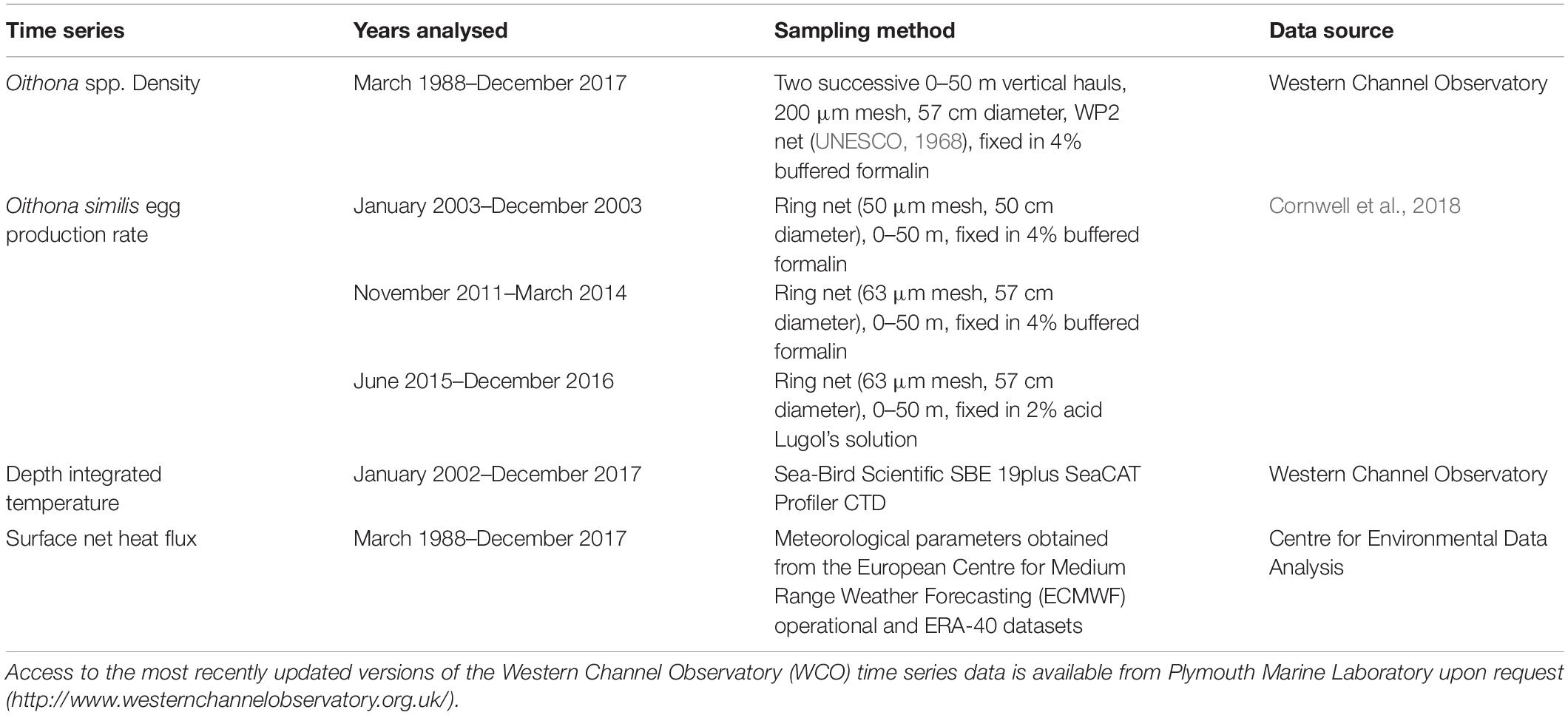
Table 1. The duration, sampling methodology, and sources of all datasets analysed in the present study.

Samples for Oithona spp. density were collected from two successive 0–50 m vertical hauls with a 200 μm mesh, 57 cm diameter WP2 net (UNESCO, 1968), and fixed in 4% buffered formalin. The category Oithona spp. comprises adults of both sexes and late stage copepodites, although the latter are not quantitatively sampled. Data derived from this long-term sampling was used to determine the day of the year at which the Oithona spp. population reached 25, 50 and 75% of the total annual cumulative density, indicating the start, middle and end of season, respectively (Mackas et al., 2012). The duration index of the population was derived from the number of days between the 25^th and 75^th cumulative percentiles. Samples for O. similis egg production rate (EPR) were collected from 0–50 m vertical hauls in 2003, and 2011 to 2016. In 2003, samples were collected using a ring net (50 μm mesh, 50 cm diameter) and fixed in 4% buffered formalin. In November 2011 to March 2014 samples were collected using a ring net (63 μm mesh, 57 cm diameter) and fixed in 4% buffered formalin. In June 2015 to December 2016 samples were collected using a ring net (63 μm mesh, 57 cm diameter) and fixed in 2% acid Lugol’s solution.

Water column temperature was determined using a Sea-Bird Scientific SBE 19plus SeaCAT Profiler CTD. Another physical parameter analysed in our study was the surface net heat flux (NHF, W m^–2) between the atmosphere and the ocean, which incorporates air-sea temperature difference, irradiance, wind speed, and stratification (Smyth et al., 2014). Surface NHF was determined using the following methodology of Smyth et al. (2014). Four processes control air-sea heat flux: shortwave radiation from the sun (QSW), outgoing longwave radiation from the sea surface (QLW), sensible heat transfer resulting from air-sea temperature differences (QSH), and latent heat transfer via evaporation of seawater (QLH). The Woods Hole Oceanographic Institution air-sea exchange MATLAB^® tools (Fairall et al., 2003) were used to determine QSW, QLW, QSH and QLH (Pawlowicz et al., 2001), in units of W m^–2. Meteorological parameters were obtained from the European Centre for Medium Range Weather Forecasting (ECMWF) ERA-40 and Operational analyses, extracted for the grid point 50°N, 4°W. These parameters were the following: air temperature (T_a,°C), dew point (T_d,°C), wind speed at 10 m (U₁₀, ms^–1), cloud fraction (CF, 0: clear; 1: overcast) and atmospheric pressure (P, mb). Sea surface temperature (SST) (T_s,°C), combined with the ECMWF data, was used to run the heat flux model for the period 1988–2018. QSW was calculated as a function of date and position with correction for CF (Reed, 1977); QLW as a function of T_a, T_s, T_d and CF using the Berliand bulk formula (Fung et al., 1984). QSH and QLH were calculated as a function of T_a, T_s, T_d, CF, P, and U₁₀. The sum of all four components results in surface NHF, with the sign convention of positive NHF being heat flux into the water column.

Plankton Sampling During 2017–2018

Sampling was conducted at mid-morning on a near-weekly basis from 18^th September 2017 to 15^th October 2018. To determine the vertical distribution of O. similis life stages, 10 L Niskin bottles were attached to a CTD rosette, and fired at depths of 2, 10, 25 and 50 m. At each depth, 10 L of water was collected and transferred from the Niskin bottle into a carboy via silicone tubing attached to the Niskin bottle valve. Triplicate seawater samples for picoplankton and small nanoplankton (≤12 μm) were collected at each depth from the same, or a subsequent, CTD cast. These samples were transferred from the Niskin bottle via silicone tubing into 250 mL polycarbonate bottles, and stored in a cool box. All samples were transported to the laboratory within 3 h of collection, and analysed immediately.

Plankton Analysis

In the laboratory, the contents of each carboy were gently decanted into 5 L beakers to ensure the sample was well-mixed. Subsequently, 250 mL sub-samples were taken for each depth and fixed in 2% acid Lugol’s solution for analysis of the composition and biomass of large nanoplankton (>12 μm) and microplankton. The remainder of the 10 L sample was concentrated down to 50–200 mL by reverse filtration using a 20 μm mesh, and fixed in 2% acid Lugol’s solution for analysis of O. similis density. These concentrated samples were settled for ∼24 h, after which the top layer was gently removed via syringe, leaving the bottom 50 mL to be settled for a further ∼15 h into a 3 mL Hydrobios^® counting chamber (Utermöhl, 1958). Following this, adult males and females, copepodites, nauplii and eggs of O. similis were enumerated under an Olympus IMT-2 inverted microscope at 40x magnification. Egg sacs of O. similis were easily identified, being relatively uniform and elongated compared to the irregular clusters of eggs produced by other sac-spawning species at L4. Both detached and attached egg sacs were counted. Egg densities were calculated as the product of the number of egg sacs and the mean number of eggs per sac. Nauplii were identified following Gibbons and Ogilvie (1933) and Lovegrove (1956). Early life stages were difficult to distinguish from those of the congener O. nana. However, as O. nana comprises just ∼7% of total Oithona spp. density at L4 (Cornwell et al., 2018), all early life stages of the genus were assumed to belong to O. similis. Nauplii and copepodites were counted separately but were not staged. For each sampling event, the median count of total O. similis across all life stages and depths was 101 individuals. The weighted mean depth (WMD) for each life stage sampled from the Niskin bottles was calculated as:

$$\text{WMD}=\mathrm{\Sigma }({\text{D}}_i\text{x}{\text{depth}}_i)/\mathrm{\Sigma }{\mathrm{D}}_i$$

Where D_i is density (ind m^–3) of a specific life stage at depth i.

To assess food availability in the water column, the 250 mL sub-samples taken to measure the composition and biomass of the large nanoplankton and microplankton were settled for ∼60 h, after which the top 225 mL was gently removed via syringe. The remaining 25 mL was then analysed using FlowCam VS-IVc (Fluid Imaging Technologies, Inc.). The FlowCam was fitted with a 10x objective and 100 μm flow cell. Images were collected using AutoImage Mode at 20 frames sec^–1. For each sampling event, the median cell count across all depths was 28382 cells. To avoid clogging, samples were passed through a 100 μm mesh before transfer into the sample funnel. Thus, our calculation of prey biomass excludes cells greater than 100 μm. Cells were classified manually using VisualSpreadsheet^® (V 4.1.95) software, and categorised as pennate diatoms, centric diatoms, large flagellates, round-shaped dinoflagellates, ellipsoid-shaped dinoflagellates, and ciliates. Chain forming diatoms were counted per chain. FlowCam data for cell volume, derived from area based diameter, were used to calculate carbon biomass for each category from the conversion equations of Menden-Deuer and Lessard (2000). As samples for FlowCam analysis were fixed with 2% acid Lugol’s solution, some cells may have shrunk or become swollen. However, biomass estimates for mixed species assemblages based on live or fixed cell volumes have been shown not to differ significantly (Menden-Deuer et al., 2001), thus no corrections were applied.

Samples for picoplankton and small nanoplankton (≤12 μm) were analysed live on an Accuri C6 flow cytometer (for details see Tarran and Bruun, 2015). Autotrophic picoeukaryotes (<3 μm) and nanoeukaryotes (2–12 μm), coccolithophores (5–8 μm), cryptophytes (4–10 μm), ‘Phaeocystis-like’ cells (5–6 μm), and ‘dinoflagellate-like’ cells (<20 μm) were grouped as ‘autotrophic flagellates,’ with heterotrophic nanoeukaryotes (2–12 μm) grouped separately. The group ‘heterotrophic bacteria’ consisted of high and low nucleic acid-containing bacteria. The final group consisted of autotrophic cyanobacteria Synechococcus. Cell volumes were generated by gravity filtering seawater samples through a series of polycarbonate membrane filters from 18 μm down to 0.2 μm. The filtrates were then analysed on the flow cytometer, and compared against a sample of unfiltered seawater. For each group, cell counts were used to calculate the percentage of cells remaining in the sample after filtration relative to the unfiltered sample. These percentages were plotted against filter pore size to create a series of sigmoid curves. Median cell size per group was estimated from the filter pore size at which 50% of cells were retained by the filter. From median cell size, cell volumes were calculated assuming the volume of a sphere as an approximation of cell shape. A carbon conversion factor of 0.22 pgC μm^–3 (Heywood et al., 2006), was applied to autotrophic flagellates (excluding coccolithophores and ‘dinoflagellate-like’ cells), heterotrophic nanoeukaryotes and Synechococcus. Coccolithophore cell density was converted to carbon biomass using a carbon conversion factor of 0.285 pgC μm^–3 (Tarran et al., 2006) to account for the higher carbon associated with coccoliths. Carbon biomass of ‘dinoflagellate-like’ cells was calculated from the carbon to volume relationship of Menden-Deuer and Lessard (2000). The carbon biomass of heterotrophic bacteria was calculated using a carbon conversion factor of 20 fgC cell^–1 (Lee and Fuhrman, 1987).

Dominant Frequency State Analysis

The physical and biological systems at L4 are strongly influenced by the annual cyclic motion of the Earth and by decadal processes (Smyth et al., 2014). DFSA is a highly accurate and efficient estimation signal analysis approach designed to resolve these cyclic Earth-system processes (Smyth et al., 2014; Barnes et al., 2015; Tarran and Bruun, 2015; Bruun et al., 2017). Here, DFSA was used to construct a predictive dynamic model of the seasonal and decadal properties of how the Oithona spp. population responds to the L4 environment. The L4 zooplankton time series provides a robust record of the dominant cyclic trend of Oithona spp. density. From the time series data (1988–2017), estimates of the primary Oithona spp. cyclic processes, and the baseline Oithona spp. dynamic, were derived using DFSA. The few data gaps were pre-process filled using a 6-week running median. An autoregressive noise model was used to distinguish the baseline Oithona spp. dynamic from noisy and unrelated processes. The physical and biological systems at L4 are influenced by natural cyclic variability on seasonal and decadal scales. Following this natural cyclic variability, the stable hysteresis assumption (Bruun et al., 2017) was applied to the DFSA-derived baseline Oithona spp. dynamic to predict the 2018 dynamic had typical environmental conditions prevailed.

Reproductive and Mortality Rate Estimation

All equations used to calculate rates of reproduction and mortality are provided in Table 2. In situ EPRs (eggs female^–1 d^–1) of O. similis were calculated from adult female and egg densities, using the egg-ratio method (Edmondson et al., 1962; Checkley, 1980). Egg hatch times were determined from the equation of Nielsen et al. (2002). Total reproductive output (TRO, eggs m^–3 d^–1) was calculated as the product of EPR and adult female density (Maud et al., 2015). The Bêlehràdek equation was used to calculate development time as a function of temperature for each life stage from egg to copepodite CV. For egg and post-hatch stages, we used the value α = 7.6998, as determined for eggs by Nielsen et al. (2002). Values for a were derived from the stage durations at 15°C in Sabatini and Kiørboe (1994). For further detail on these parameters and their application in calculating mortality rates, we refer the reader to Hirst and Ward (2008). Depth-integrated temperature was used in all calculations to incorporate the complete range of temperatures to which the population is potentially exposed.

TABLE 2

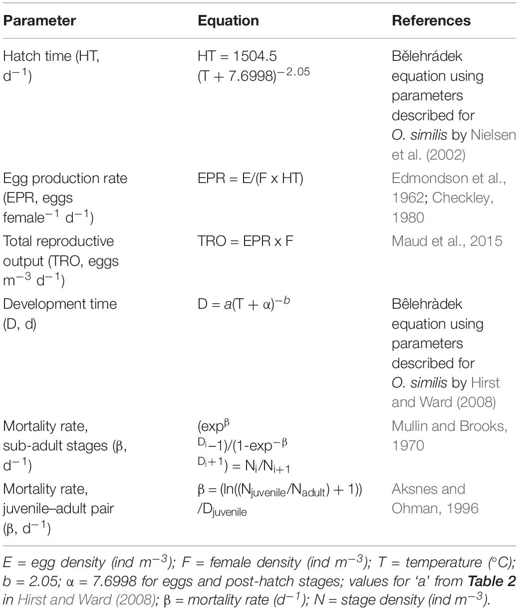
Table 2. Equations used to calculate Oithona similis reproduction and mortality rates.

Development times of each life stage were incorporated into the vertical life table (VLT) method (Mullin and Brooks, 1970; Aksnes and Ohman, 1996) to estimate mortality rates (β, d^–1) across egg, juvenile and adult stages, in consecutive pairings of these life stage categories. The VLT method determines mortality across stages from the density and duration of the stages (Aksnes et al., 1997). We grouped naupliar and copepodite stages (as juveniles), with the aim of reducing errors in estimating stage duration, indeed grouping the naupliar and copepodite stages reduced the number of negative mortality rate values seen using higher stage resolution. The primary assumption of the VLT method is that there is no trend in recruitment to a stage over the total duration of the stage pair. We therefore applied the method of Hirst et al. (2007) to determine the impact of recruitment rate on our mortality rate estimates for the egg-juvenile stage pair. Data for egg production were grouped into the periods December 2017–February 2018, March–May 2018, June–August 2018 and September–October 2018. For each period, the slope of the natural log of EPR over time was obtained via linear regression. All slopes were an order of magnitude lower than the mortality rates of the egg-juvenile stage pair, thus recruitment trends should not have significantly affected the mortality rate estimates. A major advantage of the VLT method is that it reduces the complication of advection, providing that advection equally affects all individuals in a sample (Aksnes et al., 1997), making it appropriate for our analysis.

Results

L4 Physical Environment: Time Series Comparison

The year 2018 was characterised by exceptionally low water temperatures between weeks 7 and 19, followed by a rapid rate of increase in the depth-integrated temperature at 0.41°C week^–1, from a minimum of 7.84°C in week 10, to more typical summer temperatures of 14.8°C by week 27 (Figures 1A,B). In comparison, the baseline rate of increase in mean depth-integrated temperature over the same time frame was 0.24°C week^–1 (Figure 1B). Surface NHF also underwent a rapid rate of increase (32.7 W m^–2 week^–1) in 2018, from −254 W m^–2 in week 9 to 237 W m^–2 in week 24, substantially faster than the baseline of 13.7 W m^–2 week^–1 over the same time period (Figure 1C).

FIGURE 1

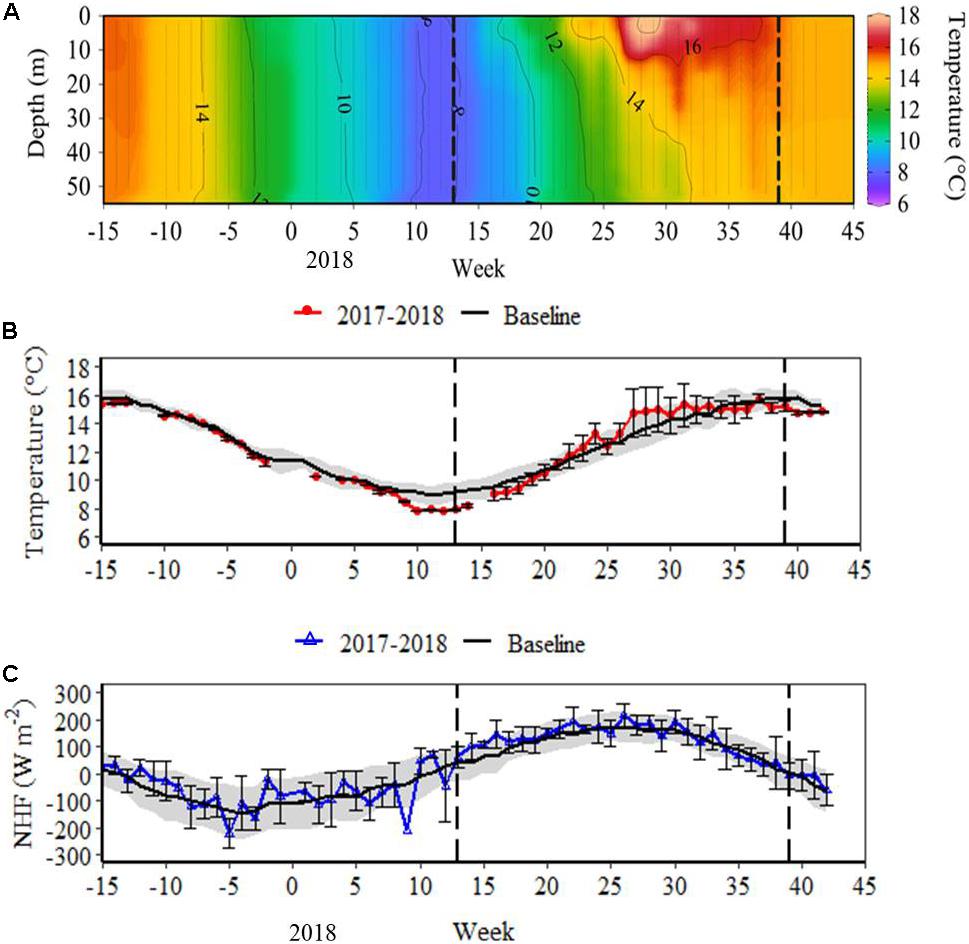
Figure 1. (A) Water column temperature for the 2017–2018 study (Ocean Data View, Schlitzer, 2018); (B) depth-integrated temperature for the 2017–2018 study and weekly mean (± SD) depth-integrated temperature for the time series baseline (2002–2017); (C) surface net heat flux (NHF) for the 2017–2018 study and weekly mean (± SD) surface NHF for the time series baseline (1988–2017). In (B,C), baseline standard deviation is represented by the grey band. Vertical dashed lines mark the onset and breakdown of stratification, indicated by the switch in surface NHF from negative to positive (week 13), and positive to negative (week 39) during the 2017–2018 study.

Oithona similis Population Dynamics: Time Series Comparison

Across the time series (1988–2018), mean (± SE) annual Oithona spp. density was generally stable (Figure 2). One exception was the year 2000, for which population densities were exceptionally high for several weeks in spring and autumn, although for most of the year densities were more typical of the time series. Linear regression analysis showed that mean annual Oithona spp. density had no significant correlation with mean annual SST or total prey biomass (P > 0.05). The day at which Oithona spp. density reached the 25^th cumulative percentile of the annual density, representing the start of the season, was not correlated with mean SST in the period February to April or May to July (P > 0.05). The duration index of the population (time between the 25^th and 75^th cumulative percentiles) ranged from 24 to 193 days. The duration index lacked any significant linear correlation with mean SST between February to April or May to July (P > 0.05). Mean annual density, timing of the start of the season and duration index of Oithona spp. also exhibited no correlation with the rate of water column stratification at the start of the season.

FIGURE 2

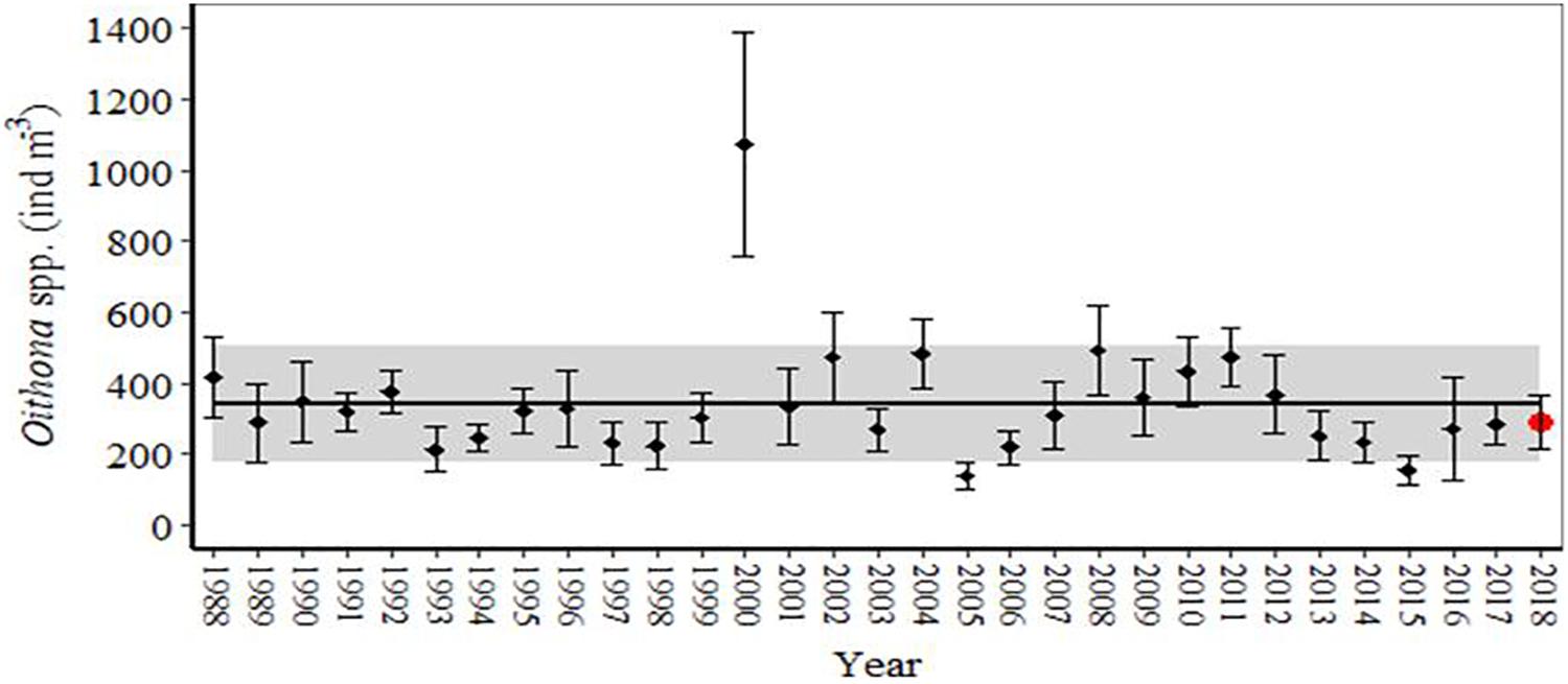
Figure 2. Mean (± SE) annual Oithona spp. density for each year of the L4 time series (1988–2018), compared against the mean (± SD) Oithona spp. density over the full time series. In the latter, the mean is represented by the solid line, and the standard deviation is represented by the grey band.

Dominant frequency state analysis determined that the statistically significant modes of variability providing the baseline seasonal climatology for both physical and biological systems at L4 were 1, 1/2 and 1/3 year cyclic processes (Figures 3A,B), plus 4 and 10.5 year cycles (Figure 3C). These five frequency states for the Oithona spp. dynamic explain 27% (R²) of the signal variability. There was no significant trend term across the 1988–2017 time series, indicating that mean Oithona spp. density has not increased or decreased across the time series. Over 1988–2017, the baseline Oithona spp. dynamic exhibited a clear bimodal cycle, with a maximum in week 20 and secondary peak in week 38 (Figure 3B). The Oithona spp. population density from the DFSA-derived 2018 prediction was 19% larger than in 2017 (Figure 3D). Timing of the spring peak in the 2017–2018 study (Figure 3E) was consistent with the DFSA-derived Oithona spp. dynamic for both the baseline (Figure 3B) and prediction (Figures 3D,E). However, the secondary peak in the 2017–2018 study for both the Niskin bottle and WP2 net data occurred several weeks earlier than the DFSA-derived prediction (Figure 3E). The median Oithona spp. density in 2018 was ∼37% larger for the Niskin bottle data than both the actual and predicted values obtained from the WP2 net data; evidence for the improved sampling efficiency of our 2017–2018 study. Due to this incompatibility between Niskin bottle and WP2 net data, we do not directly compare Oithona spp. densities between these two sampling strategies, but instead focus on the seasonal trends, which appear to be equally well-represented in both sampling strategies.

FIGURE 3

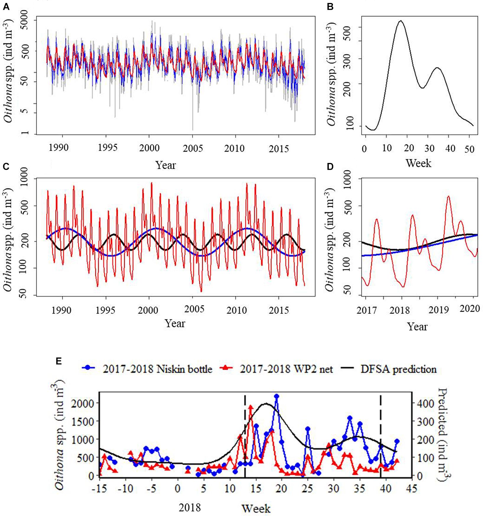
Figure 3. Dominant frequency state analysis (DFSA) of the Oithona spp. dynamic for (A) the time series (1988–2017) (grey), dominant frequency components (red), autoregressive noise components (blue); (B) the baseline Oithona spp. seasonal dynamic (1, 1/2 and 1/3 year cyclic terms) for the time series (1988–2017); (C) the dominant cyclic terms (blue: 10.5 years, black: 4 years) and baseline Oithona spp. seasonal dynamic (red) for the time series (1988–2017); (D) the DFSA-derived prediction of the Oithona spp. seasonal dynamic, lines as for (C); (E) depth-integrated density of Oithona similis adults from Niskin bottle sampling in the 2017–2018 study, Oithona spp. density from the WP2 net over the 2017–2018 study, and the DFSA-derived 2018 prediction of the Oithona spp. seasonal dynamic. Sub-figures (A–D) are on a logarithmic scale, and (E) on an absolute scale. In sub-figure (E), the DFSA 2018 prediction had reduced variability compared to the real observations, and was thus plotted on the secondary axis to aid comparison. Vertical dashed lines mark the onset and breakdown of stratification, indicated by the switch in surface NHF from negative to positive (week 13), and positive to negative (week 39) during the 2017–2018 study.

L4 Trophic Environment in 2017–2018

The pico- micro-plankton community exhibited distinct seasonality in biomass and vertical distribution (Figure 4). Ciliate carbon biomass maxima occurred in week 24, with a relatively wide depth-distribution. Subsequently, carbon biomass of round-shaped dinoflagellates exhibited a single maximum in week 32, concentrated around 10 m. Two peaks in ellipsoid-shaped dinoflagellate carbon biomass occurred between weeks 22–32 at around 25 m, followed by a third peak between weeks 36 and 38 in the 10 m layer. Diatom carbon biomass was highest between weeks 18 and 27, predominantly in the lower half of the water column. The fluorescence signal recorded by the CTD showed a corresponding depth profile over this time period, evidence that the diatom cells were alive, and not a sinking mass of a decaying bloom. Large flagellates exhibited several biomass peaks between weeks 15 and 32, reaching maximum biomass in weeks 35–38 at 10 m. The pico- nano-plankton occurred predominantly at the top 10 m of the water column, although heterotrophic taxa had a generally wider vertical distribution compared to autotrophic taxa. An initial peak in autotrophic flagellate biomass in week 27 was followed by a biomass maximum in week 38. Heterotrophic nanoeukaryotes were relatively abundant from week 26 onwards, with maximum biomass in week 35. Heterotrophic bacteria biomass has highest in weeks 24 and 35–37. Synechococcus was rare for most of the year, with a single biomass maximum in week 36. Of the above taxa, autotrophic flagellates had the greatest contribution to carbon biomass.

FIGURE 4

Figure 4. Prey carbon biomass over the 2017–2018 study (Ocean Data View, Schlitzer, 2018). Vertical dashed lines mark the onset and breakdown of stratification, indicated by the switch in surface NHF from negative to positive (week 13), and positive to negative (week 39) during the 2017–2018 study.

2017–2018 Study: Oithona similis Population Dynamics

In spring (weeks 11–22), depth-integrated mean (± SE) O. similis densities were 1750 ± 325 ind m^–3 for nauplii, 2830 ± 621 ind m^–3 for copepodites, 660 ± 167 ind m^–3 for adult females, and 82.7 ± 20.1 ind m^–3 for adult males. Over summer (weeks 23–35) these densities increased substantially in the naupliar (2080 ± 553 ind m^–3) and copepodite stages (4710 ± 966 ind m^–3), whereas the increase in adult density was negligible for both females (675 ± 144 ind m^–3) and males (84.1 ± 17.0 ind m^–3). The initial increase in O. similis population density between weeks 15 and 19 preceded that of prey biomass, whereas the population decline in weeks 35–38 occurred when prey biomass was maximal (Figure 5A). Over these time periods, mean (± SE) depth-integrated total prey carbon biomass, excluding bacteria, increased from 112 ± 17.3 to 233 ± 75.02 μg C L^–1. The O. similis population exhibited clear ontogenetic differences in vertical distribution, with all life stages being relatively scarce in the top few metres (Figure 5B). Nauplii were most abundant at 10 m, whereas copepodites had a wider depth range of 10–25 m. Adult stages had the widest depth range, occurring predominantly in the lower half of the water column. It therefore appears that the depth distribution of O. similis at L4 increases with development to later life stages.

FIGURE 5

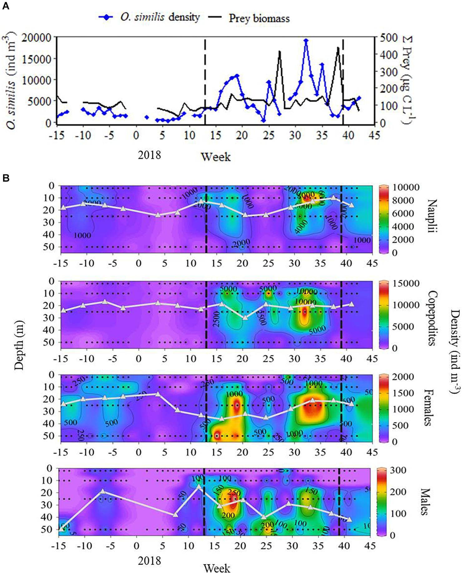
Figure 5. (A) Depth-integrated O. similis population density including all life stages, against total prey biomass, excluding bacteria, over the 2017–2018 study; (B) O. similis nauplii, copepodite, adult female, and adult male density over the 2017–2018 study (Ocean Data View, Schlitzer, 2018). Grey triangles represent weighted mean depth (WMD). Vertical dashed lines mark the onset and breakdown of stratification, indicated by the switch in surface NHF from negative to positive (week 13), and positive to negative (week 39) during the 2017–2018 study.

Reproductive and Mortality Rates

Oithona similis EPR seasonality over 2017–2018 resembled that of the baseline EPR dynamic, with minimum rates in winter, followed by an increasing trend towards maximum rates in summer (Figure 6A). In 2018, the summer maximum occurred several weeks earlier than that of the baseline EPR dynamic. However, during the summer (weeks 23–35) there was little difference between mean (± SE) EPR in 2018 (2.59 ± 0.45 eggs female^–1 d^–1) and the baseline (2.60 ± 0.35 eggs female^–1 d^–1). At the start of 2018, EPR was substantially below the baseline until approximately week 18 (Figure 6A). As TRO is a function of EPR and adult female density, direct comparison between the 2017 and 2018 study and the baseline is not possible on account of the different sampling efficiencies of the Niskin bottle and the fine mesh nets. Nonetheless, in agreement with the baseline dynamic, TRO in 2018 was highest in spring and summer (Figure 6B), coinciding with peaks in adult female density and EPR, respectively. Mortality rates (β) were considerably higher and more variable in the egg-juvenile stage pair compared to the juvenile-adult stage pair, although both exhibited an overall increase in mortality rate towards summer (Figure 6C). Maximum mortality rate for the egg-juvenile stage pair was 0.54 d^–1 in week 38. In contrast, maximum mortality rate for the juvenile-adult stage pair was just 0.19 d^–1, and occurred in week 26.

FIGURE 6

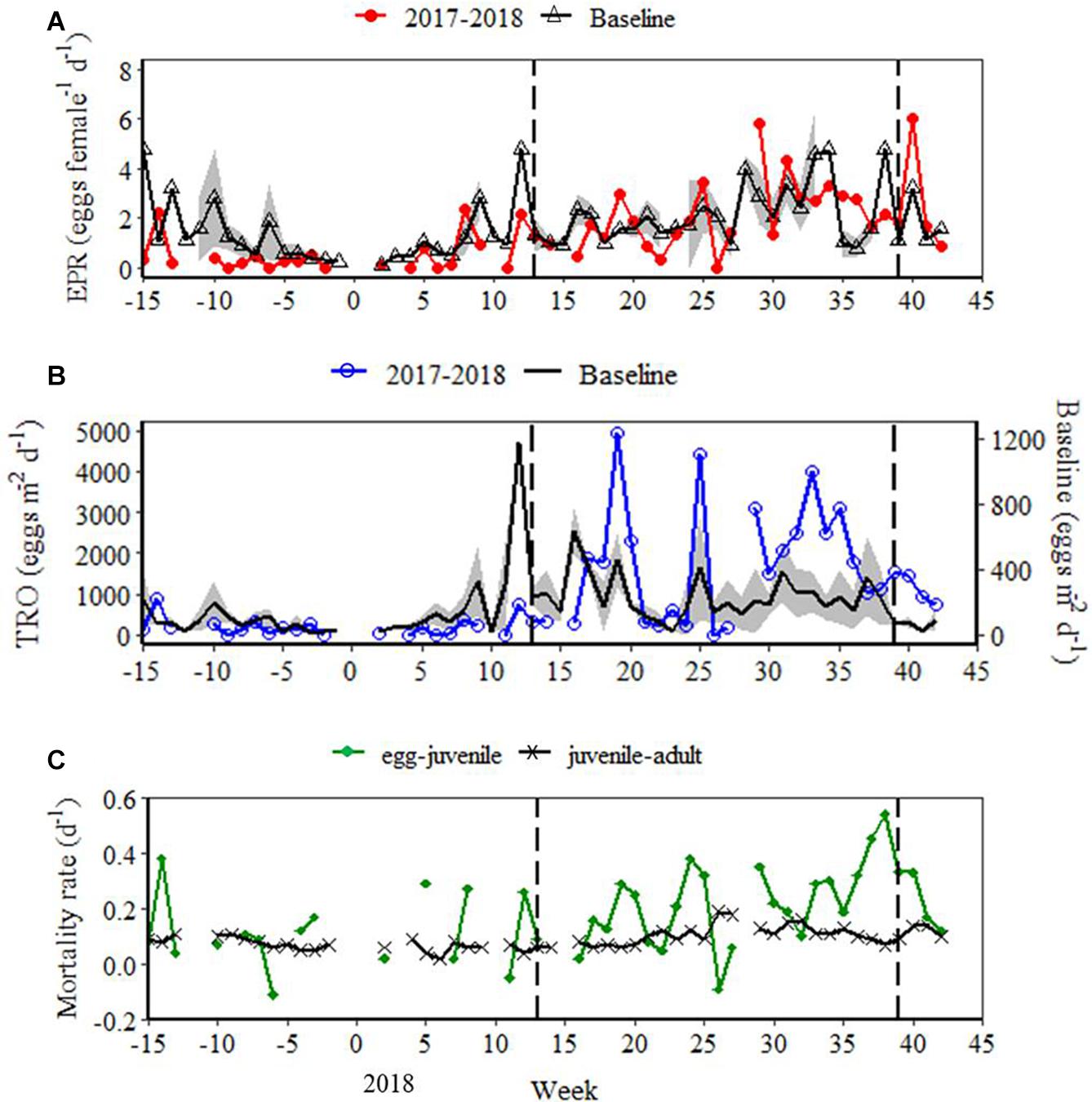
Figure 6. (A) Oithona similis egg production rate (EPR) for the 2017–2018 study and weekly mean (± SE) O. similis EPR for the time series baseline (2003; 2011–2016); (B) O. similis total reproductive output (TRO) for the 2017–2018 study and weekly mean (± SE) O. similis TRO for the time series baseline (2011–2016), note the use of different axes due to divergence in sampling efficiencies between methods; (C) mortality rates (β) of O. similis egg-juvenile and juvenile-adult stage pairs for the 2017–2018 study. In (A,B), baseline standard error is represented by the grey band. Vertical dashed lines mark the onset and breakdown of stratification, indicated by the switch in surface NHF from negative to positive (week 13), and positive to negative (week 39) during the 2017–2018 study.

Discussion

Our study shows that the numerically dominant cyclopoid species O. similis has maintained generally stable population dynamics over the L4 time series, despite high variability in both the physical and biological environment, as evidenced in our 1-year intensive study. The biomass dominant calanoid species C. helgolandicus has also maintained stable population dynamics at L4 (Maud et al., 2015). In contrast, important species at this site, such as Acartia clausi, Pseudocalanus elongatus and Temora longicornis, have undergone major declines in population density (Edwards et al., 2020). Here, we compare the population dynamics of O. similis and C. helgolandicus at L4 to investigate which traits may contribute to population stability and resilience in this highly variable environment.

Oithona similis Population Dynamics: Time Series Comparison

Despite high climatic variability over the 2017–2018 study, O. similis maintained similar population densities and bimodal cycle as that over the whole 30-year time series. Evidence of Oithona spp. population stability at L4 has been reported previously (Atkinson et al., 2015; Castellani et al., 2016; Cornwell et al., 2018). Moreover, bimodal cycles in density are reported in O. similis populations from the White and Barents Seas (Dvoretskii, 2007; Dvoretsky and Dvoretsky, 2009), Loch Striven, Scotland (Marshall, 1949), and the Southern Ocean (Fransz and Gonzalez, 1995). In contrast, a single density peak in spring (Castellani et al., 2016), summer (Zamora-Terol et al., 2014), and late autumn (Lischka and Hagen, 2005), has been documented in Mediterranean, subarctic and Arctic O. similis populations, respectively.

We found that mean SST was not correlated with either the mean annual density or phaenological timings of the L4 Oithona spp. population, supporting the results of a previous L4 time series study of Oithona spp. (Castellani et al., 2016). However, temperature is a major driver for other O. similis populations, both in terms of density (Ward and Hirst, 2007; Dvoretsky and Dvoretsky, 2009; Castellani et al., 2016), and biomass (Castellani et al., 2007). The importance of temperature in driving population dynamics may depend on the proximity of the population to their thermal range edge, with temperature effects becoming stronger closer to this edge. We conclude that at station L4, it appears temperature is, presently and historically, not the most important driver of O. similis population dynamics in terms of density or phaenology, either at the intra- or inter-annual scale.

L4 Trophic Environment

The various numerical and conceptual models developed to explain the plankton seasonality at station L4 are primarily based on trophic parameters (Atkinson et al., 2018). Considering the preference of Oithona spp. for motile prey (Atkinson, 1995, 1996; Castellani et al., 2005), the L4 Oithona spp. population has been suggested to benefit from the increased summer abundance of motile prey, such as ciliates and dinoflagellates (Kenitz et al., 2017). However, our results suggest that other factors may have a greater impact on the population dynamic. For example, the autumn decline in O. similis population density in 2017–2018 would not have been predicted based on the high biomass of motile prey at this time. Indeed, the importance of food in driving O. similis population dynamics at L4 is uncertain (Castellani et al., 2016; Cornwell et al., 2018; Djeghri et al., 2018), and we propose that other factors likely override the effect of food, as discussed below.

Vertical Profile: Population Dynamics and Trade-Offs

Depth-resolved sampling enabled us to study the vertical profile and seasonality of all O. similis life stages. Nauplii were most abundant in the 10 m layer, where pico- nano-plankton biomass was generally greatest. One explanation for this distribution is that growth is essential for survival among early life stages. Furthermore, occupying the warm upper layer would accelerate ontogenetic development, resulting in an earlier temporal onset of improved motility and escape performance, which could potentially reduce predation mortality (McLaren, 1963; Fiksen and Giske, 1995; Kiørboe and Sabatini, 1995). However, occupying the upper layer increases exposure to visual predators. There is thus a trade-off between growth and survival among earlier life stages, which potentially forces them to adopt more risky feeding behaviours (Hirst and Bunker, 2003). In contrast, our finding that adult stages occupy greater depths may reflect their ability to live for longer periods with less food (Hirst and Bunker, 2003), potentially enabling adults to reduce feeding in favour of predation avoidance. Thus, the trade-off between growth and survival may be different for adults compared to earlier life stages.

All life stages were relatively scarce in the top few metres of the water column despite periods of high food biomass in this layer. Other factors, such as ultraviolet stress (Fileman et al., 2017), visual predators and turbulence, may be forcing the population out of this layer. Although turbulence can enhance prey encounter rates for ambush predators (Kiørboe and Saiz, 1995; Saiz and Kiørboe, 1995), Oithona spp. populations have been observed to occupy greater depths during periods of increased surface turbulence (Incze et al., 2001; Visser et al., 2001; Maar et al., 2006), although nauplii may be less able to avoid turbulence due to their low swimming capacity (Lagadeuc et al., 1997; Andersen et al., 2001; Maar et al., 2003). However, considering that nauplii were also relatively rare in the uppermost layer, the impact of turbulence in determining the O. similis vertical profile at L4 is debateable. Another factor to consider is salinity, although the generally weak salinity gradient at L4 makes it unlikely that salinity has a strong impact on the O. similis vertical profile at this site. In contrast, at freshwater influenced sites, salinity can be a major driver of vertical distribution, with distinct avoidance of low salinity upper layers, as observed for all life stages of O. similis in the Bornholm Basin, Baltic Sea (Hansen et al., 2004), and Hylsfjord, Norway (Andersen and Nielsen, 2002). At other sites, the factors driving the O. similis vertical profile are less clear. For example, vertical distribution was not significantly correlated with surface salinity, temperature or chlorophyll across the North Sea (Maar et al., 2006), or with phytoplankton biomass or water column stratification in Chaleur Bay, Gulf of Saint Lawrence (Lagadeuc et al., 1997). Evidently, the factors driving O. similis vertical profile vary between populations, and depend on the environment in which each population occurs.

It must be acknowledged that in our study, all sampling events were conducted at mid-morning. Thus, our results do not account for potential diel vertical migration, although studies from other sites generally report a lack of diel vertical migration in O. similis (Turner and Dagg, 1983; Lagadeuc et al., 1997; Andersen and Nielsen, 2002; Eiane and Ohman, 2004; Hansen et al., 2004; Maar et al., 2006). However, seasonal vertical migration has been observed in the O. similis population of Kongsfjorden, Svalbard, which occurs predominantly in the upper 50 m layer in summer and below 100 m in winter (Lischka and Hagen, 2005). Conversely, we found that the vertical profile of each life stage appears relatively constant throughout the year at L4, as also reported for O. similis across the Arctic Ocean (Ashjian et al., 2003).

The Balance Between Reproduction and Mortality

Egg production rate seasonality over the 2017–2018 study was similar to the baseline dynamic, although the summer EPR maximum was several weeks earlier than that of the baseline. In sac-spawning species such as O. similis, the production of new egg clutches is limited by the rate at which the previous eggs hatch (Ward and Hirst, 2007). As higher temperatures increase rates of embryonic development and hatching, and consequently reduces the time between the production of egg clutches, EPR increases as a result (Nielsen et al., 2002). The early EPR peak in 2018 could have resulted from accelerated development of the spring cohort due to the rapid rate of seasonal warming. Coincident with the low water column temperatures at the start of 2018, EPR was substantially below the baseline seasonal average until around week 18, at which point water column temperature had begun to reach more typical levels.

Female body size of copepod species can vary substantially and also impact fecundity (Sabatini and Kiørboe, 1994). At station L4, O. similis adult female body size conforms to the temperature–size rule (Atkinson, 1994), decreasing from a maximum in spring following the low winter temperatures, to a minimum in autumn after the annual temperature maximum (Cornwell et al., 2018). The seasonal trend in O. similis female body size is therefore counter to that of EPR, indicating that for the L4 O. similis population, fecundity appears more influenced by positive temperature effects than reductions associated with smaller female body size. In contrast, EPR of the calanoid copepod C. helgolandicus at L4 is positively correlated with adult female body size, with both EPR and female body size peaking in spring (Cornwell et al., 2018). Therefore, future increases in temperature fluctuations may impact fecundity via its effects on physiology of the species, including development rates, and also body size, the strength of these effects being species specific.

The spring and summer peaks in TRO and naupliar density indicate the production of two main generations over the 2017–2018 study, conforming to the bimodal cycle of the baseline dynamic. The production of two generations per year has been previously reported in other O. similis populations (Digby, 1954; Lischka and Hagen, 2005; Dvoretskii, 2007; Dvoretsky and Dvoretsky, 2009). The small peak in naupliar density in spring 2018 coincided with maximum adult density, indicative of high recruitment early in the year. Subsequently, there was a general increase in mortality rates over the remainder of the study. Mortality rates were far greater and more variable across the egg-juvenile stage pair compared to the juvenile-adult stage pair, which agrees with previous studies on other O. similis populations reporting higher mortality rates in early life stages (Marshall, 1949; Fransz and Gonzalez, 1995; Eiane and Ohman, 2004; Hirst and Ward, 2008; Thor et al., 2008), and low recruitment success (McLaren, 1969). The high mortality rates in autumn, particularly for the egg-juvenile stage pair, may have contributed to the O. similis population decline.

What Traits Provide Population Stability in Copepods?

Despite the overall decline in copepod densities at station L4 over the 30-year time series (Edwards et al., 2020), O. similis has maintained stable population densities and seasonality. The calanoid copepod C. helgolandicus has also maintained stable population densities over the L4 time series (Maud et al., 2015; Edwards et al., 2020). The inter-annual variation in mean population densities is similar in both species, with coefficients of variation (CV) of 0.49 and 0.44 for O. similis and C helgolandicus, respectively. For context, copepods that have undergone long-term population declines at L4, namely Pseudocalanus elongatus, Temora longicornis and Acartia clausi, show greater inter-annual variability in their mean population densities, with CVs of 0.54, 0.61 and 0.71, respectively. Both O. similis and C. helgolandicus have been intensively studied at L4, providing a broad data set which we use here to suggest traits contributing to population stability (Table 3).

TABLE 3

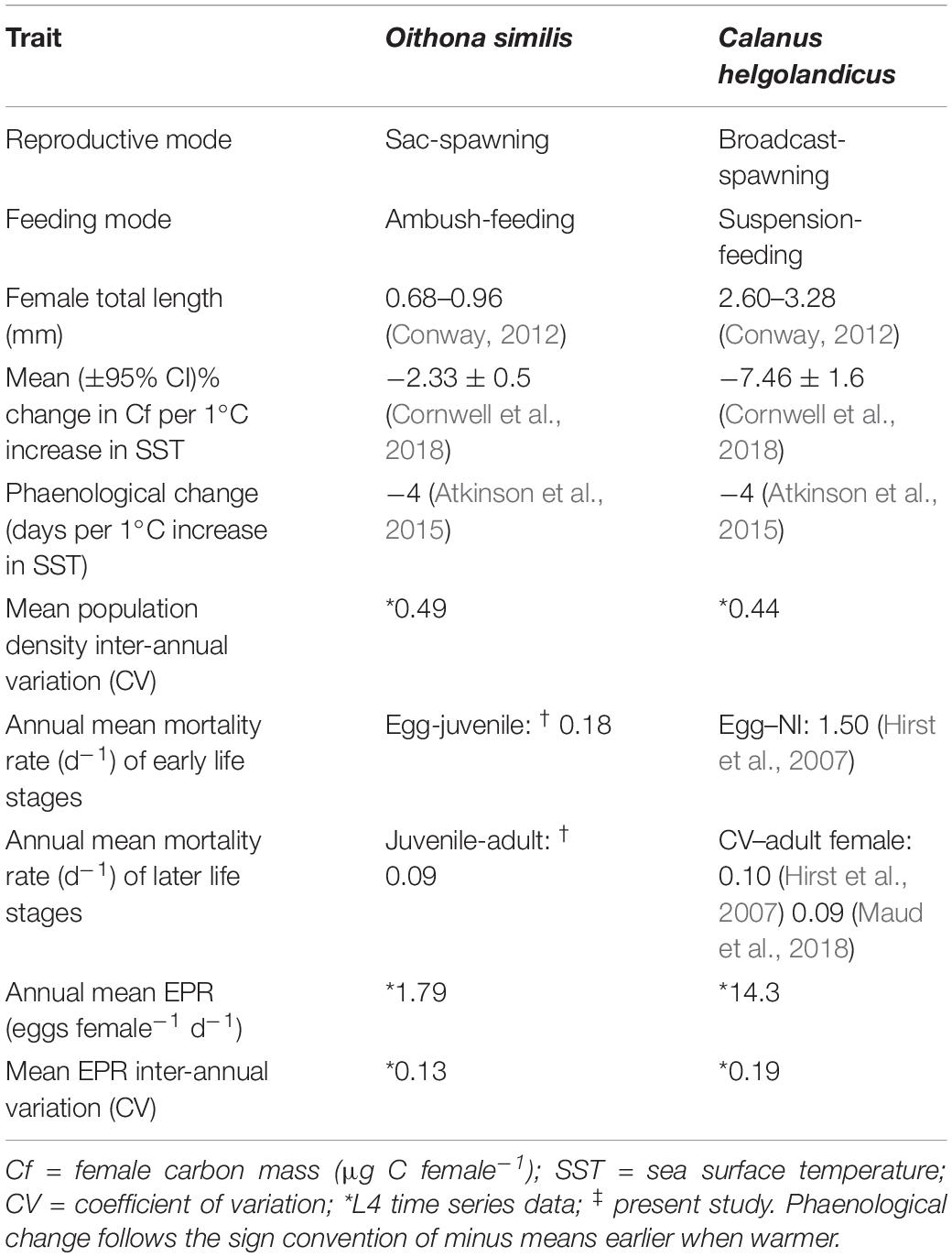
Table 3. Traits and inter-annual variability of Oithona similis and Calanus helgolandicus at station L4. Data for C. helgolandicus egg production rate (EPR) were derived from the L4 time series (1992–2018).

Oithona similis and C. helgolandicus contrast markedly in body size, feeding- and reproductive modes, with C. helgolandicus generally exhibiting greater reproductive output and high mortality in early life stages. Conversely, small cyclopoid copepods such as O. similis possess lower rates of feeding, growth, reproduction and mortality compared to calanoid species of equivalent size, and these lower rates have been suggested to contribute to the stability of cyclopoid populations (Paffenhöfer, 1993). In contrast to the bimodal cycle and summer EPR maxima of O. similis, as described in this study, the population density of C. helgolandicus at L4 follows a considerably weaker bimodal cycle with a summer maximum, and peak EPR during the spring diatom bloom (Irigoien and Harris, 2003; Maud et al., 2015). These inter-specific differences in seasonality are to some extent explained by the factors driving EPR in each species. Temperature is significantly positively correlated with EPR in O. similis at L4 (Cornwell et al., 2018) and at other sites (Ward and Hirst, 2007; Dvoretsky and Dvoretsky, 2009; Zamora-Terol et al., 2014). Conversely, C. helgolandicus EPR is more dependent on food availability than temperature (Bonnet et al., 2005), as observed in the L4 population (Maud et al., 2015; Cornwell et al., 2018). From this analysis, it is clear that species with contrasting functional traits can maintain stable population densities and seasonality.

Temperature is considered to be a fundamental driver of phaenology and species density at the macroecological scale of ocean basins (Beaugrand and Kirby, 2018; Beaugrand et al., 2019). However, at individual study sites such as L4, these temperature effects on population dynamics are less evident. For instance, the peaks in O. similis population density at L4 occur at both the coldest and warmest times of the year. At the scales of seasonal and inter-annual variability at a single site, other factors may be more important in shaping population trends. For example, density-dependent mortality processes have been suggested to provide population stability in C. helgolandicus at L4 (Hirst et al., 2007; Maud et al., 2015, 2017, 2018). Likewise, our results lead us to propose mortality as a major driver of the stable population dynamic of O. similis at L4, which is upheld even during periods of high climatic variability.

Data Availability Statement

The datasets generated for this study are available on request to the corresponding author.

Author Contributions

LC designed the methodology, performed field and laboratory work regarding data collection, analysed the data, and wrote the manuscript. EF, JB, AH, GT, HF, CL, and AA contributed to the drafting of the manuscript. EF provided support with FlowCam analysis and classification. JB significantly improved the time series analysis by introducing modelling techniques. AH provided guidance in calculating mortality rates. GT provided the flow cytometry data. TS provided the net heat flux data. AM provided the L4 zooplankton time series data.

Funding

LC was supported by a NERC GW4 + Doctoral Training Partnership studentship from the Natural Environment Research Council (NE/L002434/1). The Western Channel Observatory is funded by the United Kingdom Natural Environment Research Council through its National Capability, with AA contribution to this paper supported by Long-term Single Centre Science Programme, ‘Climate Linked Atlantic Sector Science’ (NE/R015953/1). We thank the United Kingdom Research Councils funded Models2Decisions grant (M2DPP035: EP/P01677411) and ReCICLE (NE/M00412011) project.

Conflict of Interest

The authors declare that the research was conducted in the absence of any commercial or financial relationships that could be construed as a potential conflict of interest.

Acknowledgments

We thank D. V. P. Conway for his guidance on copepod identification, J. R. Fishwick for providing the CTD data, the Centre for Environmental Data Analysis for providing the ECMWF operational and ERA-40 datasets, and the crew of the RV Plymouth Quest. The time series analysis codes for the signal analysis methods used in this paper are available from the R Core Team open access links (package TSA): www.R-project.org.

Footnotes

1. ^ http://www.westernchannelobservatory.org.uk/

References

Aksnes, D. L., Miller, C. B., Ohman, M. D., and Wood, S. N. (1997). Estimation techniques used in studies of copepod population dynamics—a review of underlying assumptions. Sarsia 82, 279–296. doi: 10.1080/00364827.1997.10413657

CrossRef Full Text | Google Scholar

Aksnes, D. L., and Ohman, M. D. (1996). A vertical life table approach to zooplankton mortality estimation. Limnol. Oceanogr. 41, 1461–1469. doi: 10.4319/lo.1996.41.7.1461

CrossRef Full Text | Google Scholar

Andersen, C. M., and Nielsen, T. G. (2002). The effect of a sharp pycnocline on plankton dynamics in a freshwater influenced Norwegian fjord. Ophelia 56, 135–160. doi: 10.1080/00785236.2002.10409495

CrossRef Full Text | Google Scholar

Andersen, V., Gubanova, A., Nival, P., and Ruellet, T. (2001). Zooplankton community during the transition from spring bloom to oligotrophy in the open NW Mediterranean and effects of wind events. 2. Vertical distributions and migrations. J. Plankton Res. 23, 243–261. doi: 10.1093/plankt/23.3.243

CrossRef Full Text | Google Scholar

Ashjian, C. J., Campbell, R. G., Welch, H. E., Butler, M., and Van Keuren, D. (2003). Annual cycle in abundance, distribution, and size in relation to hydrography of important copepod species in the western Arctic Ocean. Deep Sea Res. Part I Oceanogr. Res. Pap. 50, 1235–1261. doi: 10.1016/S0967-0637(03)00129-8

CrossRef Full Text | Google Scholar

Atkinson, A. (1995). Omnivory and feeding selectivity in five copepod species during spring in the Bellingshausen Sea, Antarctica. ICES J. Mar. Sci. 52, 385–396. doi: 10.1016/1054-3139(95)80054-9

CrossRef Full Text | Google Scholar

Atkinson, A. (1996). Subantarctic copepods in an oceanic, low chlorophyll environment: ciliate predation, food selectivity and impact on prey populations. Mar. Ecol. Prog. Ser. 130, 85–96. doi: 10.3354/meps130085

CrossRef Full Text | Google Scholar

Atkinson, A., Harmer, R. A., Widdicombe, C. E., McEvoy, A. J., Smyth, T. J., Cummings, D. G., et al. (2015). Questioning the role of phenology shifts and trophic mismatching in a planktonic food web. Prog. Oceanogr. 137, 498–512. doi: 10.1016/j.pocean.2015.04.023

CrossRef Full Text | Google Scholar

Atkinson, A., Polimene, L., Fileman, E. S., Widdicombe, C. E., McEvoy, A. J., Smyth, T. J., et al. (2018). Comment. What drives plankton seasonality in a stratifying shelf sea? Some competing and complementary theories. Limnol. Oceanogr. 63, 2877–2884. doi: 10.1002/lno.11036

CrossRef Full Text | Google Scholar

Atkinson, D. (1994). Temperature and organism size: a biological law for ectotherms? Adv. Ecol. Res. 25, 1–58. doi: 10.1016/S0065-2504(08)60212-3

CrossRef Full Text | Google Scholar

Barnes, M. K., Tilstone, G. H., Suggett, D. J., Widdicombe, C. E., Bruun, J., Martinez-Vicente, V., et al. (2015). Temporal variability in total, micro-and nano-phytoplankton primary production at a coastal site in the western English Channel. Prog. Oceanogr. 137, 470–483. doi: 10.1016/j.pocean.2015.04.017

CrossRef Full Text | Google Scholar

Beaugrand, G., Conversi, A., Atkinson, A., Cloern, J., Chiba, S., Fonda-Umani, S., et al. (2019). Prediction of unprecedented biological shifts in the global ocean. Nat. Clim. Chang. 9, 237–243. doi: 10.1038/s41558-019-0420-1

CrossRef Full Text | Google Scholar

Beaugrand, G., and Kirby, R. R. (2018). How do marine pelagic species respond to climate change? Theories and observations. Ann. Rev. Mar. Sci. 10, 169–197. doi: 10.1146/annurev-marine-121916-063304

PubMed Abstract | CrossRef Full Text | Google Scholar

Bonnet, D., Richardson, A., Harris, R., Hirst, A., Beaugrand, G., Edwards, M., et al. (2005). An overview of Calanus helgolandicus ecology in European waters. Prog. Oceanogr. 65, 1–53. doi: 10.1016/j.pocean.2005.02.002

CrossRef Full Text | Google Scholar

Bruun, J. T., Allen, J. I., and Smyth, T. J. (2017). Heartbeat of the Southern Oscillation explains ENSO climatic resonances. J. Geophys. Res. Oceans 122, 6746–6772. doi: 10.1002/2017JC012892

CrossRef Full Text | Google Scholar

Castellani, C., Irigoien, X., Harris, R. P., and Holliday, N. P. (2007). Regional and temporal variation of Oithona spp. biomass, stage structure and productivity in the Irminger Sea, North Atlantic. J. Plankton Res. 29, 1051–1070. doi: 10.1093/plankt/fbm079

CrossRef Full Text | Google Scholar

Castellani, C., Irigoien, X., Harris, R. P., and Lampitt, R. S. (2005). Feeding and egg production of Oithona similis in the North Atlantic. Mar. Ecol. Prog. Ser. 288, 173–182. doi: 10.3354/meps288173

CrossRef Full Text | Google Scholar

Castellani, C., Licandro, P., Fileman, E., Di Capua, I., and Mazzocchi, M. G. (2016). Oithona similis likes it cool: evidence from two long-term time series. J. Plankton Res. 38, 703–717. doi: 10.1093/plankt/fbv104

CrossRef Full Text | Google Scholar

Checkley, D. M. (1980). The egg production of a marine planktonic copepod in relation to its food supply: laboratory studies. Limnol. Oceanogr. 25, 430–446. doi: 10.4319/lo.1980.25.3.0430

CrossRef Full Text | Google Scholar

Conway, D. V. P. (2012). “Marine zooplankton of southern Britain. Part 2: Arachnida, Pycnogonida, Cladocera, Facetotecta, Cirripedia and Copepoda,” in Marine Biological Association of the United Kingdom, No 26, ed. A. W. G. John, (Plymouth: Occasional Publications), 163.

Google Scholar

Cornwell, L. E., Findlay, H. S., Fileman, E. S., Smyth, T. J., Hirst, A. G., Bruun, J. T., et al. (2018). Seasonality of Oithona similis and Calanus helgolandicus reproduction and abundance: contrasting responses to environmental variation at a shelf site. J. Plankton Res. 40, 295–310. doi: 10.1093/plankt/fby007

CrossRef Full Text | Google Scholar

Digby, P. (1954). The biology of the marine planktonic copepods of Scoresby Sound, East Greenland. J. Anim. Ecol. 23, 298–338. doi: 10.2307/1984

CrossRef Full Text | Google Scholar

Djeghri, N., Atkinson, A., Fileman, E. S., Harmer, R. A., Widdicombe, C. E., McEvoy, A. J., et al. (2018). High prey-predator size ratios and unselective feeding in copepods: a seasonal comparison of five species with contrasting feeding modes. Prog. Oceanogr. 165, 63–74. doi: 10.1016/j.pocean.2018.04.013

CrossRef Full Text | Google Scholar

Dvoretskii, V. G. (2007). Characteristics of the Oithona similis (Copepoda: Cyclopoida) in the White and Barents seas. Dokl. Biol. Sci. 414, 223–225. doi: 10.1134/S0012496607030167

CrossRef Full Text | Google Scholar

Dvoretsky, V. G., and Dvoretsky, A. G. (2009). Life cycle of Oithona similis (Copepoda: Cyclopoida) in Kola Bay (Barents Sea). Mar. Biol. 156, 1433–1446. doi: 10.1007/s00227-009-1183-4

CrossRef Full Text | Google Scholar

Edmondson, W. T., Comita, G. W., and Anderson, G. C. (1962). Reproductive rate of copepods in nature and its relation to phytoplankton population. Ecology 43, 625–634. doi: 10.2307/1933452

CrossRef Full Text | Google Scholar

Edwards, M., Atkinson, A., Bresnan, E., Helaouet, P., McQuatters-Gollup, A., Ostle, C., et al. (2020). Plankton, jellyfish and climate in the North-East Atlantic. MCCIP Sci. Rev. 2020, 322–353. doi: 10.14465/2020.arc15.plk

CrossRef Full Text | Google Scholar

Edwards, M., Helaouet, P., Alhaija, R. A., Batten, S., Beaugrand, G., Chiba, S., et al. (2016). Global Marine Ecological Status Report: Results from the Global CPR Survey 2014/2015. SAHFOS Technical Report No. 11. Plymouth: SAHFOS.

Google Scholar

Eiane, K., and Ohman, M. D. (2004). Stage-specific mortality of Calanus finmarchicus, Pseudocalanus elongatus and Oithona similis on Fladen Ground, North Sea, during a spring bloom. Mar. Ecol. Prog. Ser. 268, 183–193. doi: 10.3354/meps268183

CrossRef Full Text | Google Scholar

Eloire, D., Somerfield, P. J., Conway, D. V. P., Halsband-Lenk, C., Harris, R., and Bonnet, D. (2010). Temporal variability and community composition of zooplankton at station L4 in the Western Channel: 20 years of sampling. J. Plankton Res. 32, 657–679. doi: 10.1093/plankt/fbq009

CrossRef Full Text | Google Scholar

Fairall, C. W., Bradley, E. F., Hare, J. E., Grachev, A. A., and Edson, J. B. (2003). Bulk parameterization of air–sea fluxes: updates and verification for the COARE algorithm. J. Clim. 16, 571–591. doi: 10.1175/1520-0442(2003)016<0571:bpoasf>2.0.co;2

CrossRef Full Text | Google Scholar

Fiksen, Ø., and Giske, J. (1995). Vertical distribution and population dynamics of copepods by dynamic optimization. ICES J. Mar. Sci. 52, 483–503. doi: 10.1016/1054-3139(95)80062-X

CrossRef Full Text | Google Scholar

Fileman, E. S., White, D. A., Harmer, R. A., Aytan, Ü., Tarran, G. A., Smyth, T., et al. (2017). Stress of life at the ocean’s surface: latitudinal patterns of UV sunscreens in plankton across the Atlantic. Prog. Oceanogr. 158, 171–184. doi: 10.1016/j.pocean.2017.01.001

CrossRef Full Text | Google Scholar

Fransz, H. G., and Gonzalez, S. R. (1995). The production of Oithona similis (Copepoda: Cyclopoida) in the Southern Ocean. ICES J. Mar. Sci. 52, 549–555. doi: 10.1016/1054-3139(95)80069-7

CrossRef Full Text | Google Scholar

Fung, I. Y., Harrison, D. E., and Lacis, A. A. (1984). On the variability of the net longwave radiation at the ocean surface. Rev. Geophys. 22, 177–193. doi: 10.1029/RG022i002p00177

CrossRef Full Text | Google Scholar

Gibbons, S. G., and Ogilvie, H. S. (1933). The development stages of Oithona helgolandica and Oithona spinirostris with a note on the occurrence of body spines in cyclopoid nauplii. J. Mar. Biol. Assoc. U. K. 18, 529–550. doi: 10.1017/S0025315400043885

CrossRef Full Text | Google Scholar

Hansen, F. C., Möllmann, C., Schütz, U., and Hinrichsen, H. H. (2004). Spatio-temporal distribution of Oithona similis in the Bornholm Basin (central Baltic Sea). J. Plankton Res. 26, 659–668. doi: 10.1093/plankt/fbh061

CrossRef Full Text | Google Scholar

Harris, R. (2010). The L4 time-series: the first 20 years. J. Plankton Res. 32, 577–583. doi: 10.1093/plankt/fbq021

CrossRef Full Text | Google Scholar

Heywood, J. L., Zubkov, M. V., Tarran, G. A., Fuchs, B. M., and Holligan, P. M. (2006). Prokaryoplankton standing stocks in oligotrophic gyre and equatorial provinces of the Atlantic Ocean: evaluation of inter-annual variability. Deep Sea Res. Part II Top. Stud. Oceanogr. 53, 1530–1547. doi: 10.1016/j.dsr2.2006.05.005

CrossRef Full Text | Google Scholar

Highfield, J. M., Eloire, D., Conway, D. V., Lindeque, P. K., Attrill, M. J., and Somerfield, P. J. (2010). Seasonal dynamics of meroplankton assemblages at station L4. J. Plankton Res. 32, 681–691. doi: 10.1093/plankt/fbp139

CrossRef Full Text | Google Scholar

Hirst, A. G., Bonnet, D., and Harris, R. P. (2007). Seasonal dynamics and mortality rates of Calanus helgolandicus over two years at a station in the English Channel. Mar. Ecol. Prog. Ser. 340, 189–205. doi: 10.3354/meps340189

CrossRef Full Text | Google Scholar

Hirst, A. G., and Bunker, A. J. (2003). Growth of marine planktonic copepods: global rates and patterns in relation to chlorophyll a, temperature, and body weight. Limnol. Oceanogr. 48, 1988–2010. doi: 10.4319/lo.2003.48.5.1988

CrossRef Full Text | Google Scholar

Hirst, A. G., and Ward, P. (2008). Spring mortality of the cyclopoid copepod Oithona similis in polar waters. Mar. Ecol. Prog. Ser. 372, 169–180. doi: 10.3354/meps07694

CrossRef Full Text | Google Scholar

Incze, L. S., Hebert, D., Wolff, N., Oakey, N., and Dye, D. (2001). Changes in copepod distributions associated with increased turbulence from wind stress. Mar. Ecol. Prog. Ser. 213, 229–240. doi: 10.3354/meps213229

CrossRef Full Text | Google Scholar

IPCC, (2019). “Summary for policymakers,” in IPCC Special Report on the Ocean and Cryosphere in a Changing Climate, eds H.-O. Pörtner, D. C. Roberts, V. Masson-Delmotte, P. Zhai, M. Tignor, E. Poloczanska, et al. (Geneva: IPCC).

Google Scholar

Irigoien, X., and Harris, R. P. (2003). Interannual variability of Calanus helgolandicus in the English Channel. Fish. Oceanogr. 12, 317–326. doi: 10.1046/j.1365-2419.2003.00247.x

CrossRef Full Text | Google Scholar

Kenitz, K. M., Visser, A. W., Mariani, P., and Andersen, K. H. (2017). Seasonal succession in zooplankton feeding traits reveals trophic trait coupling. Limnol. Oceanogr. 62, 1184–1197. doi: 10.1002/lno.10494

CrossRef Full Text | Google Scholar

Kiørboe, T., and Sabatini, M. (1995). Scaling of fecundity, growth and development in marine planktonic copepods. Mar. Ecol. Prog. Ser. 120, 285–298. doi: 10.3354/meps120285

CrossRef Full Text | Google Scholar

Kiørboe, T., and Saiz, E. (1995). Planktivorous feeding in calm and turbulent environments, with emphasis on copepods. Mar. Ecol. Prog. Ser. 122, 135–145. doi: 10.3354/meps122135

CrossRef Full Text | Google Scholar

Lagadeuc, Y., Bouté, M., and Dodson, J. J. (1997). Effect of vertical mixing on the vertical distribution of copepods in coastal waters. J. Plankton Res. 19, 1183–1204. doi: 10.1093/plankt/19.9.1183

CrossRef Full Text | Google Scholar

Lee, S., and Fuhrman, J. A. (1987). Relationships between biovolume and biomass of naturally derived marine bacterioplankton. Appl. Environ. Microbiol. 53, 1298–1303. doi: 10.1016/0198-0254(87)96080-8

PubMed Abstract | CrossRef Full Text | Google Scholar

Lischka, S., and Hagen, W. (2005). Life histories of the copepods Pseudocalanus minutus, P. acuspes (Calanoida) and Oithona similis (Cyclopoida) in the Arctic Kongsfjorden (Svalbard). Polar Biol. 28, 910–921. doi: 10.1007/s00300-005-0017-1

CrossRef Full Text | Google Scholar

Lovegrove, T. (1956). Copepod nauplii (II). J. Cons. Cons. Int. Exp. Mer. Zooplankton Sheet 63, 1–14.

Google Scholar

Maar, M., Nielsen, T. G., Stips, A., and Visser, A. (2003). Microscale distribution of zooplankton in relation to turbulent diffusion. Limnol. Oceanogr. 48, 1312–1325. doi: 10.4319/lo.2003.48.3.1312

CrossRef Full Text | Google Scholar

Maar, M., Visser, A. W., Nielsen, T. G., Stips, A., and Saito, H. (2006). Turbulence and feeding behaviour affect the vertical distributions of Oithona similis and Microsetella norwegica. Mar. Ecol. Prog. Ser. 313, 157–172. doi: 10.3354/meps313157

CrossRef Full Text | Google Scholar

Mackas, D. L., Greve, W., Edwards, M., Chiba, S., Tadokoro, K., Eloire, D., et al. (2012). Changing zooplankton seasonality in a changing ocean: comparing time series of zooplankton phenology. Prog. Oceanogr. 97, 31–62. doi: 10.1016/j.pocean.2011.11.005

CrossRef Full Text | Google Scholar

Marshall, S. M. (1949). On the biology of the small copepods in Loch Striven. J. Mar. Biol. Assoc. U. K. 28, 45–113. doi: 10.1017/S0025315400055235

CrossRef Full Text | Google Scholar

Maud, J. L., Atkinson, A., Hirst, A. G., Lindeque, P. K., Widdicombe, C. E., Harmer, R. A., et al. (2015). How does Calanus helgolandicus maintain its population in a variable environment? Analysis of a 25-year time series from the English Channel. Prog. Oceanogr. 137, 513–523. doi: 10.1016/j.pocean.2015.04.028

CrossRef Full Text | Google Scholar

Maud, J. L., Atkinson, A., Hirst, A. G., White, D., Lindeque, P. K., and Widdicombe, C. E. (2017). Calanus helgolandicus in the Western English Channel: Population Dynamics and the Role of Mortality. Doctoral dissertation, Queen Mary University of London, London.

Google Scholar

Maud, J. L., Hirst, A. G., Atkinson, A., Lindeque, P. K., and McEvoy, A. J. (2018). Mortality of Calanus helgolandicus: sources, differences between the sexes and consumptive and nonconsumptive processes. Limnol. Oceanogr. 63, 1741–1761. doi: 10.1002/lno.10805

CrossRef Full Text | Google Scholar

McLaren, I. A. (1963). Effects of temperature on growth of zooplankton, and the adaptive value of vertical migration. J. Fish. Res. Board Can. 20, 685–727. doi: 10.1139/f63-046

CrossRef Full Text | Google Scholar

McLaren, I. A. (1969). Population and production ecology of zooplankton in Ogac Lake, a landlocked fiord on Baffin Island. J. Fish. Res. Board Can. 26, 1485–1559. doi: 10.1139/f69-139

CrossRef Full Text | Google Scholar

Menden-Deuer, S., and Lessard, E. J. (2000). Carbon to volume relationships for dinoflagellates, diatoms, and other protist plankton. Limnol. Oceanogr. 45, 569–579. doi: 10.4319/lo.2000.45.3.0569

CrossRef Full Text | Google Scholar

Menden-Deuer, S., Lessard, E. J., and Satterberg, J. (2001). Effect of preservation on dinoflagellate and diatom cell volume and consequences for carbon biomass predictions. Mar. Ecol. Prog. Ser. 222, 41–50. doi: 10.3354/meps222041

CrossRef Full Text | Google Scholar

Mullin, M. M., and Brooks, E. R. (1970). The ecology of the plankton off La Jolla, California, in the period April through September, 1967. Part VII. Production of the planktonic copepod, Calanus helgolandicus. Bull. Scripps Inst. Oceanogr. 17, 89–103. doi: 10.1002/ecy.1804

PubMed Abstract | CrossRef Full Text | Google Scholar

Nielsen, T. G., Møller, E. F., Satapoomin, S., Ringuette, M., and Hopcroft, R. R. (2002). Egg hatching rate of the cyclopoid copepod Oithona similis in arctic and temperate waters. Mar. Ecol. Prog. Ser. 236, 301–306. doi: 10.3354/meps236301

CrossRef Full Text | Google Scholar

Nielsen, T. G., and Sabatini, M. (1996). Role of cyclopoid copepods Oithona spp. in North Sea plankton communities. Mar. Ecol. Prog. Ser. 139, 79–93. doi: 10.3354/meps139079

CrossRef Full Text | Google Scholar

O’Brien, T. D., Lorenzoni, L., Isensee, K., and Valdés, L. (eds). (2017). What are Marine Ecological Time Series Telling us About the Ocean? A Status Report. IOC-UNESCO, IOC Technical Series No. 129. Paris: IOC.

Google Scholar

Paffenhöfer, G. A. (1993). On the ecology of marine cyclopoid copepods (Crustacea, Copepoda). J. Plankton Res. 15, 37–55. doi: 10.1093/plankt/15.1.37

CrossRef Full Text | Google Scholar

Pawlowicz, R., Beardsley, R., Lentz, S., Dever, E., and Anis, A. (2001). Software simplifies air-sea data estimates. Eos Trans. 82:2. doi: 10.1029/01EO00004

CrossRef Full Text | Google Scholar

Reed, R. K. (1977). On estimating insolation over the ocean. J. Phys. Oceanogr. 7, 482–485. doi: 10.1175/1520-0485(1977)007<0482:oeioto>2.0.co;2

CrossRef Full Text | Google Scholar

Sabatini, M., and Kiørboe, T. (1994). Egg production, growth and development of the cyclopoid copepod Oithona similis. J. Plankton Res. 16, 1329–1351. doi: 10.1093/plankt/16.10.1329

CrossRef Full Text | Google Scholar

Saiz, E., and Kiørboe, T. (1995). Predatory and suspension feeding of the copepod Acartia tonsa in turbulent environments. Mar. Ecol. Prog. Ser. 122, 147–158. doi: 10.3354/meps122147

CrossRef Full Text | Google Scholar

Schlitzer, R. (2018). Ocean Data View. Available at: https://odv.awi.de (accessed October 28, 2019).

Google Scholar

Smyth, T. J., Allen, I., Atkinson, A., Bruun, J. T., Harmer, R. A., Pingree, R. D., et al. (2014). Ocean net heat flux influences seasonal to interannual patterns of plankton abundance. PLoS One 9:e98709. doi: 10.1371/journal.pone.0098709

PubMed Abstract | CrossRef Full Text | Google Scholar

Tarran, G. A., and Bruun, J. T. (2015). Nanoplankton and picoplankton in the Western English Channel: abundance and seasonality from 2007–2013. Prog. Oceanogr. 137, 446–455. doi: 10.1016/j.pocean.2015.04.024

CrossRef Full Text | Google Scholar

Tarran, G. A., Heywood, J. L., and Zubkov, M. V. (2006). Latitudinal changes in the standing stocks of nano-and picoeukaryotic phytoplankton in the Atlantic Ocean. Deep Sea Res. Part II Top. Stud. Oceanogr. 53, 1516–1529. doi: 10.1016/j.dsr2.2006.05.004

CrossRef Full Text | Google Scholar

Thor, P., Nielsen, T. G., and Tiselius, P. (2008). Mortality rates of epipelagic copepods in the post-spring bloom period in Disko Bay, western Greenland. Mar. Ecol. Prog. Ser. 359, 151–160. doi: 10.3354/meps07376

CrossRef Full Text | Google Scholar

Turner, J. T. (2004). The importance of small planktonic copepods and their roles in pelagic marine food webs. Zool. Stud. 43, 255–266.

Google Scholar

Turner, J. T., and Dagg, M. J. (1983). Vertical distributions of continental shelf zooplankton in stratified and isothermal waters. Biol. Oceanogr. 3, 1–40. doi: 10.1080/01965581.1983.10749470

CrossRef Full Text | Google Scholar

UNESCO, (1968). Monographs on Oceanographic Methodology: Zooplankton Sampling. Paris: United Nations.

Google Scholar

Utermöhl, H. (1958). Methods of collecting plankton for various purposes are discussed. SIL Commun. 9, 1–38. doi: 10.1080/05384680.1958.11904091

CrossRef Full Text | Google Scholar

Visser, A. W., Saito, H., Saiz, E., and Kiørboe, T. (2001). Observations of copepod feeding and vertical distribution under natural turbulent conditions in the North Sea. Mar. Biol. 138, 1011–1019. doi: 10.1007/s002270000520

CrossRef Full Text | Google Scholar

Ward, P., and Hirst, A. G. (2007). Oithona similis in a high latitude ecosystem: abundance, distribution and temperature limitation of fecundity rates in a sac spawning copepod. Mar. Biol. 151, 1099–1110. doi: 10.1007/s00227-006-0548-1

CrossRef Full Text | Google Scholar

White, D. A., Widdicombe, C. E., Somerfield, P. J., Airs, R. L., Tarran, G. A., Maud, J. L., et al. (2015). The combined effects of seasonal community succession and adaptive algal physiology on lipid profiles of coastal phytoplankton in the Western English Channel. Mar. Chem. 177, 638–652. doi: 10.1016/j.marchem.2015.10.005

CrossRef Full Text | Google Scholar

Widdicombe, C. E., Eloire, D., Harbour, D., Harris, R. P., and Somerfield, P. J. (2010). Long-term phytoplankton community dynamics in the Western English Channel. J. Plankton Res. 32, 643–655. doi: 10.1093/plankt/fbp127

PubMed Abstract | CrossRef Full Text | Google Scholar

Zamora-Terol, S., Kjellerup, S., Swalethorp, R., Saiz, E., and Nielsen, T. G. (2014). Population dynamics and production of the small copepod Oithona spp. in a subarctic fjord of West Greenland. Polar Biol. 37, 953–965. doi: 10.1007/s00300-014-1493-y

CrossRef Full Text | Google Scholar