A General Methodology for Beached Oil Spill Hazard Mapping

1. Introduction

Risk assessments have been widely employed by scientists and engineers as a tool to deal with harmful natural events (e.g., earthquakes) and anthropogenic events (e.g., oil spills) that we are unable to describe and/or predict with fully deterministic methods. A critical step within a risk assessment framework (e.g., ISO 31000), hazard quantification (or hazard mapping) is the probabilistic estimation on the frequency of occurrence and magnitude, based on historical observations of the events of interest. The seminal paper by Gutenberg and Richter (1944) clearly illustrates how the careful analysis of the probability distribution function (PDF) of seismic events, i.e., the probability of observing an earthquake of a certain magnitude in a limited area over time, led to an objective hazard quantification method and triggered comparisons within different tectonic areas around the globe (Shedlock et al., 2000). This well-established seismic hazard framework suggests that an appropriate statistical description of the variable of interest is of fundamental importance to classify hazard and then risk. As far as the authors are aware, there has been no study dedicated to the description of beached (or floating) oil concentration PDF, based on either simulated or observed data.

The oil spill hazard assessment framework lags behind these well-established hazard assessment fields. There is a severe lack of observational data, especially oil concentrations along coasts after spill events (in the paper also referred to as beached oil concentrations), eliminating the possibility of empirically describing the coastal oil hazard. Numerical ensemble oil spill modeling has been widely used to tackle the data gap, emulating reality, i.e., spill fate and generating information for hazard quantification (e.g., Price et al., 2003; Liubartseva et al., 2015; Sepp Neves et al., 2015; French-McCay et al., 2018). However, there is currently no standard way to describe the beached oil concentrations obtained by the ensemble experiments and, therefore, mapping the relative coastal hazard. Consequently, we are still unable to compare different hazard estimates, to evaluate objectively the completeness of the ensemble datasets and, most importantly, to be able to establish a global coastal oil spill hazard assessment framework.

The estimation of the probability distribution functions of atmospheric state variables and tracer/contaminant concentrations has attracted the attention of meteorologists for decades. It has long been recognized that wind speed PDFs fit a Weibull distribution (Justus et al., 1976; Pavia and O'Brien, 1986; Monahan, 2006), characterized by a large number of low magnitude events (e.g., low wind speed), large variance and, most interestingly, “anomalously” frequent high magnitude events, typical of fat-tailed distributions. Observational and modeling experiments (Tirabassi et al., 1991a,b) have shown that wind speed plays a major role in shaping tracer concentration distributions, which were also found to fit a Weibull PDF. In the ocean, recent papers have documented that surface coastal currents (Ashkenazy and Gildor, 2011), i.e., Gulf of Eilat/Aqaba, and global ocean currents (Chu, 2009) also fit a Weibull distribution, suggesting that ocean pollutants could also be similarly distributed as observed in the atmosphere.

The linkage between flow field characteristics and tracer concentration PDFs has been described by, among others, Hu and Pierrehumbert (2001) for stratospheric flows. They explain that every flow feature (e.g., eddies, filaments) has its own characteristics such as its shape and length, speed and direction, and how long it will last before disappearing/merging with other structures. Tracer concentration PDFs are primarily a result of different “parcels separation rates” taking place in the different parts of the concentration field, modulated by the flow field features they are exposed to. Areas with a relatively complex circulation are expected to present both features with lower (e.g., western boundary currents) and higher (e.g., filaments or eddies) “separation rates.” In other words, as the flow field becomes complex and rich in features, the tracer concentration PDF increasingly depart from a Gaussian distribution. Therefore, we expect that if ocean feature-rich current patterns are Weibull distributed, the marine tracers concentrations, including beached oil, should be similarly distributed.

Recently Alves et al. (2016b) gave evidence that ocean current conditions determine the fate of the oil at the coasts. Currents are by themselves affected by bathymetry and they contain the information about the specific flow field that is consistent with the coastline constraint and the other forcings. In this paper we add to these findings by estimating the PDF of accidental oil releases, both at sea and along the coasts. Our definition is the one of “standard” accidental oil releases, corresponding to a volume of oil spilt equal to 10,000 tons, as pointed out but the analysis of Huijer (2005). Firstly, we will show that at the surface and in the open ocean, far from coastal boundaries, the oil concentration fits a Weibull PDF. Secondly we will simulate an ensemble of oil releases near the coasts and we will analyze the PDF of the beached oil. Three very different Atlantic coastline segments and ocean current regime areas will be considered for different current and wind conditions during the year 2013. A Weibull PDF function is estimated from the data and a coastal oil spill hazard index will be proposed in terms of the “Weibull tail distribution.”

After a description of the framework for oil spill hazard (section 2) and the ensemble experiments performed (section 3), the statistical distribution of oil concentrations in surface waters is analyzed (section 4). In section 5 we will then analyze the PDF for the beached oil on three coastlines around the Atlantic basin. Section 6 will offer the analysis of a new hazard indicator extracted from the statistical distributions of the beached oil in the three areas. Final overview of the results and future work is presented in section 7.

2. Standardized Approach to Evaluate Oil Spill Hazard

The framework for oil spill hazard and risk assessment has been defined by adapting the generic and recognized standard, i.e., ISO 31000, to oil spill model simulations so that the oil spill hazard assessment could be carried out in a scientific and standard way (Sepp Neves et al., 2015). The authors identify ensemble oil spill simulations as the method to produce the basic data to estimate the hazard.

Later, the technique of ensemble oil simulations was extensively analyzed for one coastal stretch, the Algarve coastal area in Portugal (Sepp Neves et al., 2016). The ensemble simulations were carried out using an extensive identification of modeling uncertainty sources: the meteo-oceanographic fields used for the oil spill simulations (different wind and ocean models were used), the inclusion of the Stokes drift, the oil spill release points, the oil spill model setup in terms of volume of oil spilled, time of spillage, and duration of the spill. Ten different model configurations were used to obtain the hazard of the beached oil at the Algarve coasts. The paper concludes that the beached oil distribution is non-Gaussian so that a hazard risk index which would use mean and standard deviations is not appropriate. In the same paper, Sepp Neves et al. (2016) show also a probability distribution of beached events that is analog of the pdf discussed and revealed in this paper (see Figure 10 of Sepp Neves et al., 2016). However, the specific PDF was not identified, and the hazard index not clarified.

In this paper we extend the simulations to 3 different coastal areas and to the open ocean, trying to show the generic character of the pdf resulting from the oil spill simulations as defined in Sepp Neves et al. (2015), Sepp Neves et al. (2016). In this paper we choose only to sample the uncertainties connected with the oil release points and the meteo-oceanographic conditions, together with the structure of the coastline. We consider operational volumes of oil spilt equal for all three areas. As shown in Sepp Neves et al. (2016) the inclusion of Stokes drift does not change the structure of the resulting beached oil PDF so we have not included the uncertainty connected to the Stokes drift.

The methodology of oil spill hazard mapping requires an extensive number of simulations due to the large number of uncertainties connected with oil spill conditions and model parameters. One principle of importance is the statistical independence of each release point simulation with respect to meteo oceanographic conditions that are responsible for the transformation and transport of the oil. In Sepp Neves et al. (2016) and in this paper we use the spatial and temporal decorrelation time of ocean mesoscale eddies as the threshold for successive simulations, but other criteria might be used if higher frequency ocean processes, such as tides, will be considered in the future. Furthermore, the length of the simulation should be a good compromise with ocean currents statistical independence and weathering processes time scale that has been estimated to be of the order of few days for similar amount of oil and duration of the spill (Coppini et al., 2011).

In this paper we would like to show that, independently from the coastal geometry, the beached oil PDF has the same structure, changing its parameters in dependence of the flow field characteristics and the wind induced transformations. The three areas considered in this study have very different mean current regimes: the Eastern Atlantic Archipelago is characterized by a relatively weak and broad southwestward flow, the Western Atlantic Island is characterized by the intense zonal Caribbean current flow and the Basilian coastal stretch is characterized by a western boundary current regime. Given these differences, the three areas differ greatly for the spatial scales and intermittency of the mesoscale eddy field, as well as the wind regimes.

3. Ensemble Experiment Setup

Ensemble oil spill simulations have been used in the past to assess hazard at the coasts and in the open sea (Price et al., 2003; Liubartseva et al., 2015; Sepp Neves et al., 2015; Olita et al., 2019) but surprisingly not much has been done with respect to the derived oil concentration frequency distributions. Here we use an ensemble simulation approach to define the PDFs for oil spill release events occurring near the coasts.

Our ensemble methodology consists of varying the oil release positions, changing the met-ocean conditions and collecting the concentration of oil either in the open ocean or along the coasts. This methodology allows to sample the uncertainty in hazard mapping due to the unknown location of the spill and different meteo-oceanographic conditions. Hazard mapping deriving from a sufficiently large number of met-ocean conditions and release points is then used to describe the PDF of oil pollution events at the coasts.

The oil spill transport and transformation model is MEDSLIK-II that solves an advection-diffusion equation for the oil concentration and its transformation processes (De Dominicis et al., 2013). The transformation of oil (or weathering) considers evaporation, emulsification, dispersion, and spreading processes connected to the slick. The advection-diffusion part of the equation is solved by a series of lagrangian equations for the position increments, $d\overrightarrow{x}$, of the parcels that compose the slick at the surface, e.g.,

$\begin{array}{ll}d\overrightarrow{x}=U(\overrightarrow{x},t)dt+\sqrt{2\kappa dt}\overrightarrow{z}(t)& (1)\end{array}$

where $\overrightarrow{x}=(x,y)$ is the horizontal position of the parcels, dt is the time increment, $U(\overrightarrow{x},t)$ is the two dimensional ocean transport field, κ is a constant horizontal turbulent diffusivity value and $\overrightarrow{z}(t)$ are independent random numbers normally distributed, parameterizing lagrangian diffusion. The model considers only surface releases, the slick is evolved considering four type of parcels: surface, dispersed, sedimented and beached parcels. For the surface parcels, Equation (1) is used with a prescribed κ (taken to be equal to 2 m²s⁻¹ and current velocity analysis fields, as described in Table 1. Earlier studies (Dominicis et al., 2014) of lagrangian diffusivities found κ ~ 1 − 100 m²s⁻¹ and here we have chosen the lowest value possible in order to diminish the importance of diffusion with respect to advection by the currents. The dispersed particles are generated by the oil transformation processes (De Dominicis et al., 2013), they evolve separately from the surface oil parcels and they compose a volume of submerged oil that we do not consider in this paper except if the dispersed oil becomes beached oil. In MEDSLIK-II oil transformation processes are associated only to density, expressed as American Petroleum Institute (API) gravity.

TABLE 1

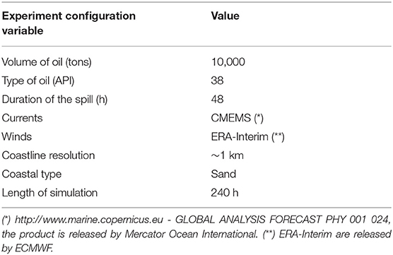
Table 1. Configuration of the ensemble experiments for the three areas of the Eastern Atlantic archipelago, the Western Atlantic Island and the Brazilian state of Bahia.

Oil parcels arriving at the coasts become beached oil parcels when their trajectories cross pre-defined coastal segments. The permanent beaching and the probability of wash-off will depend on the coastal type, as explained in De Dominicis et al. (2013), however the coastal oil holding capacity is the same for all types of coasts and it is currently set to 5, 000 bbl/km. In our analysis we use the total beached oil, the sum of the permanent and re-detachable oil. The simplistic beaching model is in accordance with the limited temporal and spatial resolution of the employed meteo-oceanographic models and in the past it has generated satisfactory results in real spill cases at similar scales (Coppini et al., 2011).

All experiments are carried out supposing several Release Points (RP) off the coastlines (Figure 1). The RP grid encompasses the main maritime routes simulating potential oil releases from the maritime corridors. Given the amount of oil released, 10⁴ tons (Table 1), our simulations encompass the release from potential accidents (Huijer, 2005). The current field $U(\overrightarrow{x},t)$ used in (1) is derived from the surface analysis fields of the Copernicus Marine Environment Service (CMEMS) at 1/12° spatial resolution (Lellouche et al., 2013)¹. The atmospheric winds and air temperature used in the weathering processes are derived from the European Center for Medium range Weather Forecast (ECMWF) ERA-Interim at 1/8° (Dee et al., 2011). The input winds are given every 6 h and linearly interpolated to the oil spill model time step which is 1 h.

FIGURE 1

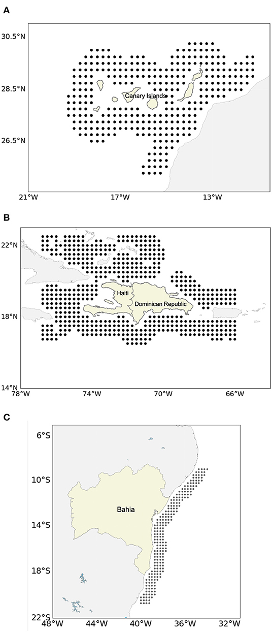
Figure 1. Map of release points (black dots) for the (A) Eastern Atlantic Archipelago, (B) the Western Atlantic Island, and (C) coastline of Bahia (Brazil).

For each release point, 240 h-long oil spill simulations were launched every 10 days throughout year 2013, using the experiment configuration described in Table 1 for three different areas in the Atlantic ocean. All different areas used the same wind and ocean current data set, the same spilled volume, type and duration of the spill (see Table 1). The coastline segments were derived from the global Wessel and Smith (1996) data set which represent the coastlines with polygons of a few hundred meters resolution for the world ocean. Coastal segments were considered at 1 km resolution for the three study areas because this is recommended if details of the coastline are not known from complementary in situ data.

The statistical independence of each release point simulation, i.e., the occurrence of one beached oil event not affecting the probability of occurrence of the other due to the same release point, was preserved in two ways. Firstly, the time interval between consecutive simulations from a single release point was longer than the typical Lagrangian decorrelation time in the Atlantic ocean (~5 days, see Maximenko et al., 2012). Secondly, the distance between neighboring release points (i.e., 25 km) was chosen based on estimation of the mesoscale spatial decorrelation scale from satellite altimetry that is at its minimum 50 km (Le Traon et al., 1990). The 10 days long simulations were chosen as a good compromise between this statistical independence and the transformation processes occurring at the surface that will evaporate and disperse the oil in the first few days for the amount and modalities of oil released in the simulations (2 days release time of 10,000 tons), as shown for example in Coppini et al. (2011).

4. The Open Ocean Surface Oil Concentrations PDF

The first aim of the paper is to show the PDF of surface oil in the open ocean, due to a single oil spill event repeated every 10 days for the entire year 2013. A single release point is chosen off the Portuguese coast, located in the open ocean flow field (Figure 2A) using the model configuration described in Table 1. The experiment considers a “virtual” coastline, sampling line, defined 50 km southward of this release point, where the oil concentration is monitored to study its statistical distribution due to the oil advective-diffusive dynamics with and without the oil transformation processes (weathering and no-weathering experiments). All non-zero surface oil concentration values observed along the sampling line grid cells are stored every 6 h throughout the duration of each simulation.

FIGURE 2

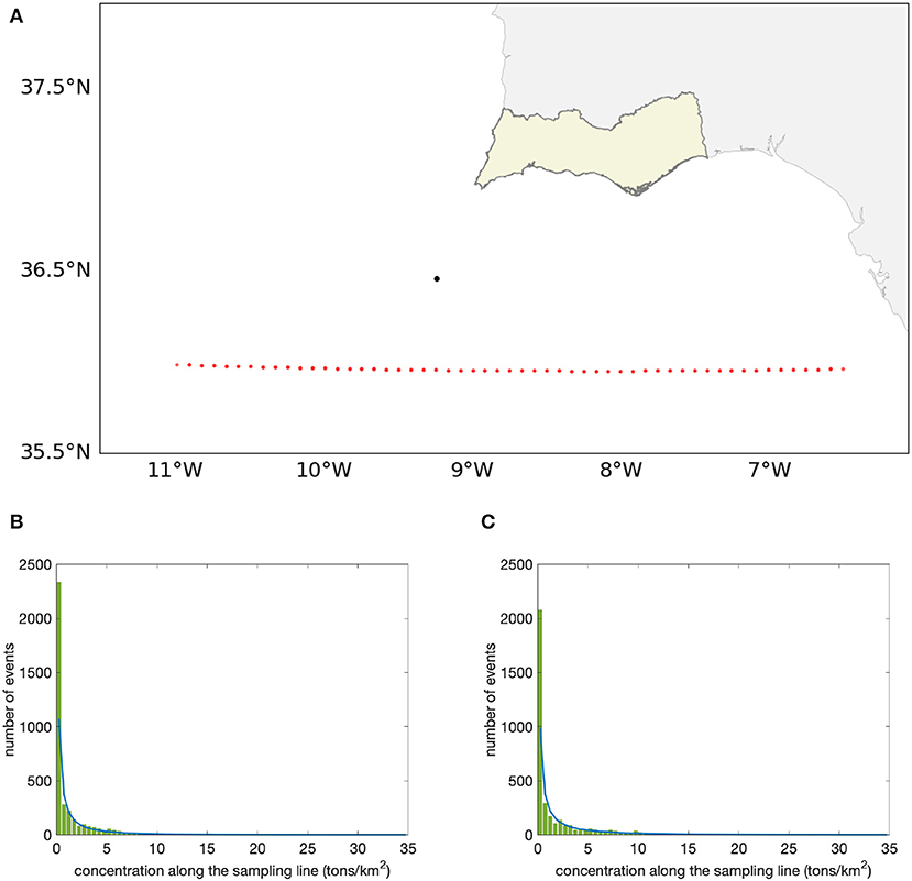
Figure 2. (A) Map of the single release point (black dot) off the Algarve with the “sampling line” drawn in red dots. Histograms and Weibull function estimation for oil concentrations obtained at the “sampling line” (B) for the weathering experiment, which includes transport and weathering processes and (C) for the no-weathering experiment.

In total, weathering and no-weathering experiments generated 3,779 non-zero oil concentration values each along the sampling line grid boxes and their concentration histograms are presented in Figure 2. Both histograms show that most of the events accumulated in low concentration bins but that in general, the range of concentrations observed is large, spanning two orders of magnitude for the oil concentration. Very high concentration events were found to be present, depicting a fat-tailed histogram.

Based on the histogram characteristics we choose a Weibull distribution function, W(x; β, η) for a maximum likelihood estimation of the PDF:

$\begin{array}{ll}W(x;\beta ,\eta )=\frac{\beta }{\eta }{\left(\frac{x}{\eta }\right)}^{\beta -1}exp{\left(-\frac{x}{\eta }\right)}^{\beta }& (2)\end{array}$

where x is the oil concentration, β and η are the shape and scale parameters respectively. In the Weibull function (2), the shape parameter is the one that controls how different from a Gaussian distribution is the PDF. For β less than 1 the distribution has its maximum at values close to zero. For β = 1 it is an exponential and for β greater than 1 the distribution has a single maximum for oil concentrations for relative large positive values and exhibits a marked asymmetry.

The Weibull distribution function has a wide range of applicability and it was in fact invented by Weibull and Stockholm (1951) to describe the failure of mechanical systems under various types of stresses or the size distribution of fly ash. Here we show for the first time that the surface oil in the ocean fits the same distribution as the currents (Chu, 2009; Ashkenazy and Gildor, 2011). It is interesting also to note that the Langevin-type equations, like the ones used in our oil spill modeling equations (1), produce probability distribution functions that are skewed and heavy-tailed (Sardeshmukh and Penland, 2015). Thus it seems likely that an active ocean tracer, such as oil, would fit a statistical distribution with a heavy tail, i.e., have a distinct non-Gaussian behavior.

The estimate of (2) to the sampling line events is shown in Figure 2 demonstrating that Weibull is a good distribution function for the oil arriving at the sampling line. The estimated shape parameter value is β = 0.399 ± 0.005, indicating a large peak at the low concentrations, for the weathering and no-weathering simulations. The scale parameter is instead different between weathering and no-weathering simulations because it is connected to the distribution mean value and it is η = 0.50 ± 0.03 tons/km² and η = 0.93 ± 0.06 tons/km² for the weathering and no-weathering experiment respectively.

We conclude that the oil concentration distribution from a single point source release and along an offshore sampling line has the form of a Weibull distribution that is peaked around the lowest concentrations.

5. The Beached Oil Concentration PDF

In this section we will show that, notwithstanding the complexity of beached oil processes, the beached oil distribution along the coastlines of three different areas in the Atlantic has a universal structure similar to the surface oil PDF found along the sampling line in the open ocean (section 4).

Following the experimental set up described in section 3, we collect the beached oil parcels on each segment of the coastline for each run. The number of RP points in the three areas are reported in Table 2 together with the number of simulations and beached oil events in each area. In Figure 3, we present the histograms of the beached oil concentration distributions for the Eastern Atlantic Archipelago, Western Atlantic Island, and state of Bahia (Brazil) coastlines.

TABLE 2

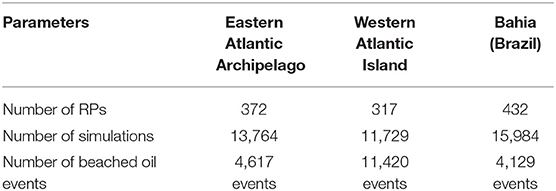
Table 2. Number of Release Points (RPs), simulations and beached oil events for year 2013 for the the three different areas.

FIGURE 3

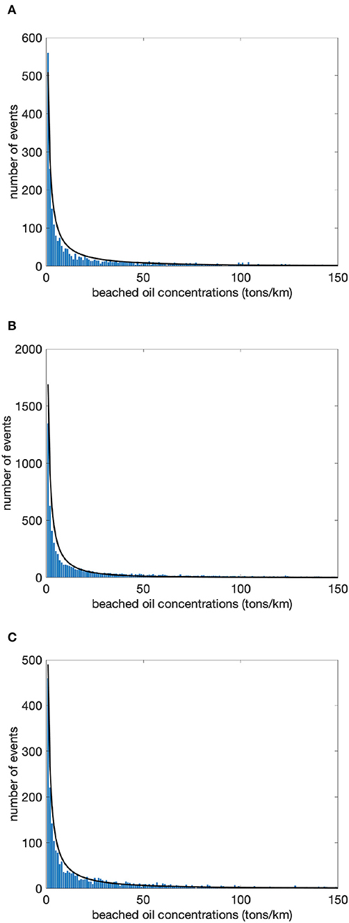
Figure 3. Histogram (blue bars) and Weibull distribution function estimation (solid black line) of beached oil concentrations from the ensemble simulations for (A) the Eastern Atlantic Archipelago, (B) the Western Atlantic Island, and (C) coast of Bahia (Brazil).

The Weibull distribution function seems to estimate well the beached oil data, even if some discrepancies appear at concentration values between 0 and 50 tons/km. The scale, η, and shape, β, parameters are reported in Table 3. It is clear again that the shape parameter is less than 0.5 for all the three areas, showing that the maximum number of events occur at the lowest values of the distribution. It is puzzling that the shape value is the same for all the areas, within the calculated errors, and it is also similar to the one found for the open sea conditions in section 4. We argue that our results show that the beached oil distribution does not depend on the specific coastal geometry but only on the type of flow field conditions that impinge on the coasts. The coastal currents are themselves affected by the type of bathymetry and coastline, so the dependence is indirect. Furthermore the beached oil PDF depends also on the winds, both directly and indirectly: the former through the transformation processes and the latter because currents are themselves driven by winds.

TABLE 3

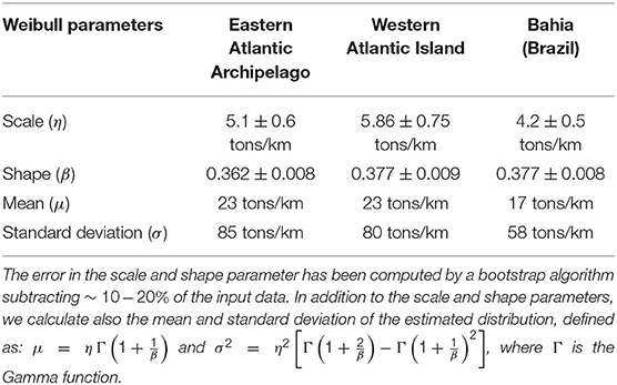
Table 3. Weibull distribution parameters emerging from the maximum likelihood estimation.

The histograms shown in Figure 3 could be also displayed on a logarithmic scale that would enhance the fat tail structure of the three distributions (Figures 4A,C,E). To check visually if our data set comes from a population that would logically be fit by a 2-parameter Weibull distribution we use the Weibull plot (Nelson, 1982). It is clear from Figures 4B,D,F that the assumption of a Weibull distribution is reasonable and that there are no outliers.

FIGURE 4

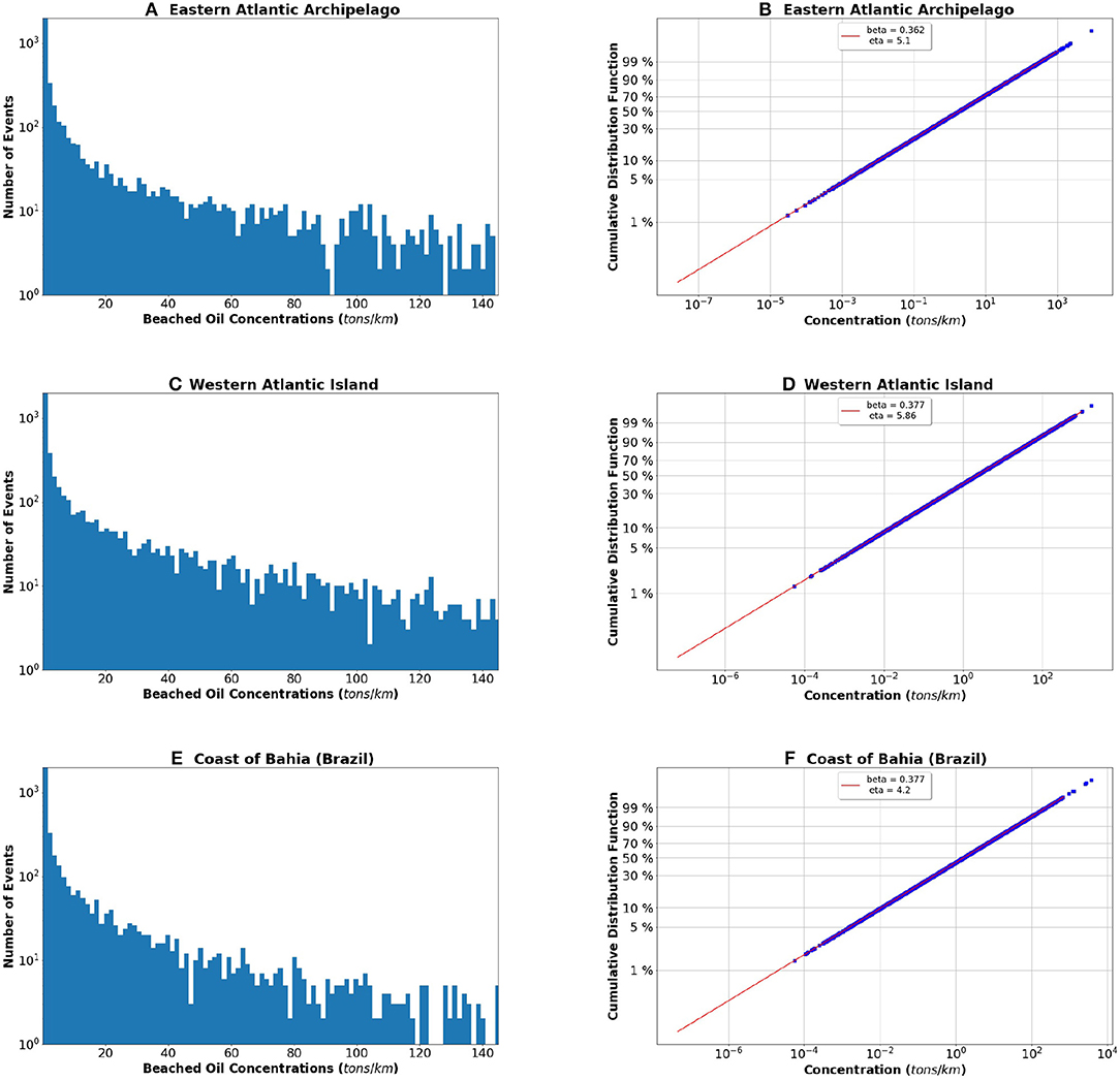
Figure 4. (A,C,E) The histogram for each of the three study areas, the Eastern Atlantic Archipelago, the Western Atlantic Island, and the Bahia coasts respectively, displayed with a logarithmic scale. (B,D,F) The Weibull plot with the cumulative distribution function $F(x)=1-e^{-{(\frac{x}{\eta })}^{\beta }}$ in the ordinates and the concentration x in the abscissa, both displayed on a logarithmic scale.

In Table 3, we list also the mean and standard deviation of the distributions from the estimated Weibull function. The Eastern Atlantic Archipelago and Western Atlantic island have similar “mean” value of beached oil concentration, i.e., 23 tons/km, while Bahia ~30% less, i.e., 17 tons/km. We conclude that the mean value of beached oil, due to surface current transport and wind induced transformations, is quite different between the two northern Atlantic areas and Bahia.

The mean of Weibull distributions with a β parameter smaller than 1 is shifted toward low concentrations. Thus, the distribution mean is not really sufficient to assess the hazard which should consider also the large events in the PDF tail. In order to do so we need to consider the cumulative distribution and define an appropriate indicator.

6. A General Indicator of Coastal Oil Spill Hazard

We will now show how beached oil concentration PDFs can be used to describe the hazard in a general way, paving the way for a quantitative method to answer a key question related to the management of the oil spill risk: what is the beached oil spill hazard for different areas and which area has the highest hazard?

Having now the PDF which describes the beached oil events from a set of RPs, simulating potential releases from accidents, we can define an index that contains the information about the large pollution events, concentrating on the tail of the Weibull distribution. It is indeed reasonable to assume that the hazard of large oil releases near the coasts should be evaluated by estimating the extreme events of the distribution.

To describe the extreme events it is then necessary to find how many events are contained in the tail with respect to the overall distribution events. To this end, we can use the Weibull tail distribution H, defined as:

$\begin{array}{ll}H=1-F(x_{cut})=e^{-{(\frac{x_{cut}}{\eta })}^{\beta }}& (3)\end{array}$

where F(x_cut) is the Weibull cumulative distribution function for the beached oil concentration x for which x ⩽ x_cut. When H is large, it means the distribution tails contain a relatively large number of high concentration events, thus the hazard is large while the contrary is true for small values of H.

The key parameter here is the threshold value x_cut chosen for the estimation of extreme events. For illustrative purposes, a concentration of 25 tons/km was applied following the International Tanker Owners Pollution Federation (ITOPF) Technical Information Paper on “Recognition of oil on shorelines” (ITOPF, 2011). The threshold is proposed for classifying impacted coastlines as heavily oiled.

The tail distribution H was computed for each area (Table 4) for the chosen value of the threshold. The Western Atlantic island emerges as an area of relatively high hazard with respect to the Eastern Atlantic Archipelago and the Bahia areas. This means that large beached oil events are more likely to occur in the Western Atlantic island, about ~ 12 − 14% more frequently than in the Eastern Atlantic Archipelago and the Bahia coasts, within the limitations of our ensemble simulations, in particular the length of the simulation and the distribution of RP.

TABLE 4

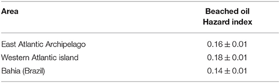
Table 4. Beached oil hazard index calculated with Equation (3) for the three areas and the threshold value of 25 tons/km.

7. Conclusions

This paper develops a straightforward and objective method to quantify the coastal oil spill hazard based on ensemble oil spill experiments which sample the uncertainties associated with oil spill accidental releases in the ocean areas next to the coasts. Ocean current variability at the mesoscales affects the flow field and in order to have a realistic sampling of the oil transport variability, ensemble simulations have been extended for an entire year, sampling the seasonal variability of the flow field at mesoscale permitting resolution.

It has been found that both oil in the open ocean and beached oil concentrations are successfully described by the Weibull distribution. Such distribution is characterized for these cases by a shape parameter which is less than 1, thus having the maximum beached oil events at small concentrations. The large beach oil concentrations are contained in a “fat tail” which characterizes this distribution. Concentrations at the coasts span two orders of magnitude values, from 1 to 100 tons/km. Previous studies have indicated that also the winds, currents, and tracers in the atmosphere and oceans distribute as Weibull but this has never been shown for active ocean pollutants, such as oil.

Furthermore, the paper proposes a new hazard index for beached oil which allows to intercompare different world ocean areas and estimate the different hazards. The index is based upon the fit of a Weibull PDF to the simulation data and extracting the tail distribution for large events.

We would like to point out that the present study has potential limitations due to the relatively low number of uncertainties considered in our simulations. In the future, experiments should probably vary the simulation length, should check different oil types and beaching algorithms and use different meteo-oceanographic conditions including higher frequency winds and tides.

This paper does not discuss how exactly the flow field modulates the oil spill hazard through advection-diffusion processes in the ocean. Nor our oil spill hazard estimates for the three regions examined are conclusive for future management decisions, especially due to the limited number of oceanographic-weather conditions considered in the study. Such estimates can be obtained with the methodology described here, but will require more extensive investigation and analyses. It is important here that a common quantitative framework for intercomparison of different world ocean areas has been found. Furthermore, to evaluate risk, vulnerability data need to be acquired and used to modulate the hazard that we have computed here (Alves et al., 2016a).

Future work will consider an in-depth study of the ocean flow field parameters and how they modulate the coastal oil spill hazard. Additionally, the spatial resolution of the oceanographic-weather fields used in our experiment offers reliable answers only for mesoscale dominated flows and coarsely resolved coastal morphology and bathymetry. The increase in resolution of the ocean and atmospheric models, and therefore their ability to reproduce smaller scale features and higher frequency variability, should impact the oil concentration PDF and, consequently, the oil spill hazard estimates. Furthermore, uncertainties connected to the amount of oil released should be also considered in the future, i.e., cases of larger oil spill releases.

Data Availability Statement

The datasets generated for this study are available on request to the corresponding author.

Author Contributions

All authors contributed to conception and design of the study. AS generated the database and wrote the first draft of the manuscript. NP and AN wrote sections of the manuscript and fully revised the manuscript. FT made the additional figure on the revised manuscript and discussed the meaning. All authors contributed to manuscript revision, read and approved the submitted version.

Funding

This work has received funding from the European Union's Horizon 2020 research and innovation program under grant agreement No. 633211, project AtlantOS.

Conflict of Interest

The authors declare that the research was conducted in the absence of any commercial or financial relationships that could be construed as a potential conflict of interest.

Acknowledgments

Special thanks to the Helenic National Meteorological Service for supplying the wind fields used in the experiment.

Footnote

1. ^http://marine.copernicus.eu/ – GLOBAL ANALYSIS FORECAST PHY 001 024, the product is released by Mercator Ocean International.

References

Alves, T. M., Kokinou, E., Zodiatis, G., and Lardner, R. (2016a). Hindcast, gis and susceptibility modelling to assist oil spill clean-up and mitigation on the southern coast of cyprus (eastern mediterranean). Deep Sea Res. Part II Top. Stud. Oceanogr. 133, 159–175. doi: 10.1016/j.dsr2.2015.07.017

CrossRef Full Text | Google Scholar

Alves, T. M., Kokinou, E., Zodiatis, G., Radhakrishnan, H., Panagiotakis, C., and Lardner, R. (2016b). Multidisciplinary oil spill modeling to protect coastal communities and the environment of the eastern mediterranean sea. Sci. Rep. 6:36882. doi: 10.1038/srep36882

PubMed Abstract | CrossRef Full Text | Google Scholar

Ashkenazy, Y., and Gildor, H. (2011). On the probability and spatial distribution of ocean surface currents. J. Phys. Oceanogr. 41, 2295–2306. doi: 10.1175/JPO-D-11-04.1

CrossRef Full Text | Google Scholar

Chu, P. C. (2009). Statistical characteristics of the global surface current speeds obtained from satellite altimetry and scatterometer data. IEEE J. Sel. Top. Appl. Earth Observ. Remote Sens. 2, 27–32. doi: 10.1109/JSTARS.2009.2014474

CrossRef Full Text | Google Scholar

Coppini, G., De Dominicis, M., Zodiatis, G., Lardner, R., Pinardi, N., Santoleri, R., et al. (2011). Hindcast of oil-spill pollution during the lebanon crisis in the eastern mediterranean, july–august 2006. Mar. Pollut. Bull. 62, 140–153. doi: 10.1016/j.marpolbul.2010.08.021

PubMed Abstract | CrossRef Full Text | Google Scholar

De Dominicis, M., Pinardi, N., Zodiatis, G., and Lardner, R. (2013). MEDSLIK-II, a Lagrangian marine oil spill model for short-term forecasting - Part 1 - Theory. Geosci. Model Dev. Discuss. 6, 1949–1997. doi: 10.5194/gmdd-6-1949-2013

CrossRef Full Text | Google Scholar

Dee, D. P., Uppala, S. M., Simmons, A. J., Berrisford, P., Poli, P., Kobayashi, S., et al. (2011). The era-interim reanalysis: configuration and performance of the data assimilation system. Q. J. R. Meteorol. Soc. 137, 553–597. doi: 10.1002/qj.828

CrossRef Full Text | Google Scholar

Dominicis, M. D., Falchetti, S., Trotta, F., Pinardi, N., Giacomelli, L., Napolitano, E., et al. (2014). A relocatable ocean model in support of environmental emergencies. Ocean Dyn. 64, 667–688. doi: 10.1007/s10236-014-0705-x

CrossRef Full Text | Google Scholar

French-McCay, D., Crowley, D., Rowe, J. J., Bock, M., Robinson, H., Wenning, R., et al. (2018). Comparative risk assessment of spill response options for a deepwater oil well blowout: Part 1. Oil spill modeling. Mar. Pollut. Bull. 133, 1001–1015. doi: 10.1016/j.marpolbul.2018.05.042

PubMed Abstract | CrossRef Full Text | Google Scholar

Gutenberg, B., and Richter, C. (1944). Frequency of earthquakes in California. Bull. Seismol. Soc. Am. 34, 185–188.

Google Scholar

Hu, Y., and Pierrehumbert, R. T. (2001). The advection-diffusion problem for stratospheric flow. Part I: concentration probability distribution function. J. Atmos. Sci. 58, 1493–1510. doi: 10.1175/1520-0469(2001)058<1493:TADPFS>2.0.CO;2

CrossRef Full Text | Google Scholar

Huijer, K. (2005). Trends in Oil Spills From Tanker Ships 1995-2004. Technical report, ITOPF Ltd.

Google Scholar

ITOPF (2011). Recognition of Oil on Shorelines. Technical report, ITOPF.

Justus, C. G., Hargraves, W. R., and Yalcin, A. (1976). Nationwide assessment of potential output from wind-powered generators. J. Appl. Meteorol. 15, 673–678. doi: 10.1175/1520-0450(1976)015<0673:NAOPOF>2.0.CO;2

CrossRef Full Text | Google Scholar

Le Traon, P. Y., Rouquet, M. C., and Boissier, C. (1990). Spatial scales of mesoscale variability in the north atlantic as deduced from geosat data. J. Geophys. Res. Oceans 95, 20267–20285. doi: 10.1029/JC095iC11p20267

CrossRef Full Text | Google Scholar

Lellouche, J.-M., Le Galloudec, O., Drévillon, M., Régnier, C., Greiner, E., Garric, G., et al. (2013). Evaluation of global monitoring and forecasting systems at Mercator Océan. Ocean Sci. 9, 57–81. doi: 10.5194/os-9-57-2013

CrossRef Full Text | Google Scholar

Liubartseva, S., De Dominicis, M., Oddo, P., Coppini, G., Pinardi, N., and Greggio, N. (2015). Oil spill hazard from dispersal of oil along shipping lanes in the southern adriatic and northern ionian seas. Mar. Pollut. Bull. 90, 259–272. doi: 10.1016/j.marpolbul.2014.10.039

PubMed Abstract | CrossRef Full Text | Google Scholar

Maximenko, N., Hafner, J., and Niiler, P. (2012). Pathways of marine debris derived from trajectories of lagrangian drifters. Mar. Pollut. Bull. 65, 51–62. doi: 10.1016/j.marpolbul.2011.04.016

PubMed Abstract | CrossRef Full Text | Google Scholar

Monahan, A. H. (2006). The probability distribution of sea surface wind speeds. Part I: theory and seawinds observations. J. Clim. 19, 497–520. doi: 10.1175/JCLI3640.1

CrossRef Full Text | Google Scholar

Nelson, W. (1982). Applied Life Data Analysis. Wiley Series in Probability and Mathematical Statistics. New York, NY: John Wiley & Sons, Inc.

Google Scholar

Olita, A., Fazioli, L., Tedesco, C., Simeone, S., Cucco, A., Quattrocchi, G., et al. (2019). Marine and coastal hazard assessment for three coastal oil rigs. Front. Mar. Sci. 6:274. doi: 10.3389/fmars.2019.00274

CrossRef Full Text | Google Scholar

Pavia, E. G., and O'Brien, J. J. (1986). Weibull statistics of wind speed over the ocean. J. Clim. Appl. Meteorol. 25, 1324–1332.

Google Scholar

Price, J. M., Johnson, W. R., Marshall, C. F., Ji, Z.-G., and Rainey, G. B. (2003). Overview of the oil spill risk analysis (OSRA) model for environmental impact assessment. Spill Sci. Technol. B 8, 529–533. doi: 10.1016/S1353-2561(03)00003-3

CrossRef Full Text | Google Scholar

Sardeshmukh, P. D., and Penland, C. (2015). Understanding the distinctively skewed and heavy tailed character of atmospheric and oceanic probability distributions. Chaos 25:036410. doi: 10.1063/1.4914169

PubMed Abstract | CrossRef Full Text | Google Scholar

Sepp Neves, A. A., Pinardi, N., and Martins, F. (2016). IT-OSRA: applying ensemble simulations to estimate the oil spill risk associated to operational and accidental oil spills. Ocean Dyn. 66, 939–954. doi: 10.1007/s10236-016-0960-0

CrossRef Full Text | Google Scholar

Sepp Neves, A. A., Pinardi, N., Martins, F., Janeiro, J., Samaras, A., Zodiatis, G., et al. (2015). Towards a common oil spill risk assessment framework - Adapting ISO 31000 and addressing uncertainties. J. Environ. Manage. 159, 158–168. doi: 10.1016/j.jenvman.2015.04.044

PubMed Abstract | CrossRef Full Text | Google Scholar

Shedlock, K. M., Giardini, D., Grunthal, G., and Zhang, P. (2000). The GSHAP global seismic hazard map. Seismol. Res. Lett. 71:679. doi: 10.1785/gssrl.71.6.679

CrossRef Full Text | Google Scholar

Tirabassi, T., Fortezza, F., and Vandini, W. (1991a). Wind circulation and air pollutant concentration in the coastal city of Ravenna. Energy Build. 16, 699–704. doi: 10.1016/0378-7788(91)90040-A

CrossRef Full Text | Google Scholar

Tirabassi, T., Mandrioli, P., and Manco, D. (1991b). Statistical distribution of airborne pollen grains. Grana 30, 255–259. doi: 10.1080/00173139109427807

CrossRef Full Text | Google Scholar

Weibull, W., and Stockholm, S. (1951). A Stiatistical Distributio Function of Wide Applicability. Technical Report 51-A-6, The American Society of Mechanical Engineers.

Google Scholar

Wessel, P., and Smith, W. H. F. (1996). A global, self-consistent, hierarchical, high-resolution shoreline database. J. Geophys. Res. 101, 8741–8743. doi: 10.1029/96JB00104

CrossRef Full Text | Google Scholar