Non-breaking Wave Effects on Buoyant Particle Distributions

1. Introduction

Plastic pollution in the ocean is ubiquitous. It is found across ocean basins, in the deep-sea, and along our coasts. The estimated sources of plastic into the ocean exceed the current amount of plastic measured in the ocean (Jambeck et al., 2015; Geyer et al., 2017); this discrepancy has become a subject of interest in the scientific community. Solving this question of “missing plastic” requires both accurate measurements and a thorough understanding of oceanic microplastics sources and sinks.

Because a large fraction of plastic in the ocean is buoyant, microplastics measurements are frequently conducted at the surface of the ocean. Direct observations are representative of the microplastic concentration at the time of sampling. However, concentrations are a function of the local conditions: on a calm day, the buoyant plastic can aggregate at the surface, but strong winds can disperse plastic throughout the mixed layer. To address this variability, large-eddy simulations of buoyant particles at the ocean surface have been conducted to show how microplastics can redistribute due to turbulent mixing by wind, currents, breaking waves, and Langmuir circulation (Brunner et al., 2015; Kukulka and Brunner, 2015; Liang et al., 2018). While these studies have provided valuable insight into how particles distribute throughout the ocean mixed layer, they are not wave-phase or free surface resolving; rather, they rely on parameterizations to include wave-averaged effects (see Chamecki et al., 2019 for a review). In reality, observations at the surface of the ocean are taken by a sampling apparatus that experiences individual wave events and an unsteady free surface. If waves induce phase variability in microplastics concentrations, and waves are not sampled uniformly, bias in the observations can result. Therefore, by studying buoyant particle distributions without wave-averaging, we are able to see important phenomena that may affect how we interpret data from free-surface net tow sampling.

A large body of work has studied the numerous ways in which waves affect surface transport and mixing processes. Waves induce a net drift in the direction of the waves, referred to as Stokes drift (see van den Bremer and Breivik, 2018 for a review); this drift is known to be important for microplastics transport from coastal shelf to oceanic scales (Isobe et al., 2014; Onink et al., 2019). Furthermore, the properties of the particles, such as inertia and shape, have also been shown to be relevant to their transport in waves (Eames, 2008; DiBenedetto et al., 2018). The ability of a wave field to disperse horizontal tracer particles has been studied as well (Herterich and Hasselmann, 1982). With regard to buoyant particles in waves, simulations similar to the ones reported here were conducted by Boufadel et al. (2006), who demonstrated how waves affect oil droplet plumes. Waves have also been studied in relation to ocean mixing through turbulence induced by wave orbital motion (Babanin, 2006). However, the effects of waves on the equilibrium distributions of buoyant particles has to our knowledge, not yet been reported.

In addition to hydrodynamic conditions, observations can be affected by the microplastic sampling method, e.g., net tows, grab samples, or filtering pumps (Hidalgo-Ruz et al., 2012; Prata et al., 2019). Some work has been done to address variability in measurements across methods (e.g., Setälä et al., 2016; Barrows et al., 2017; Karlsson et al., 2019); these studies have demonstrated that net tows can both under-sample and over-sample relative to other measurement techniques. While net tows are ideally conducted under calm conditions (e.g., sea states with Beaufort scales of 0–2) (Viršek et al., 2016), microplastics observations have been reported from conditions with Beaufort scales up to 5 (Eriksen et al., 2014; Kooi et al., 2016; Poulain et al., 2019). Therefore, moderate waves are often encountered during net tows.

Neuston (surface) net tows are conducted by trawling a net over a transect at the surface of the ocean. Captured particles are identified and counted in order to monitor microplastics surface concentrations. As sampling methods evolve and improve, understanding the variability and uncertainty in historic datasets is still necessary when analyzing temporal trends of microplastic pollution. Many longterm datasets are from observations taken with surface net tows (Law, 2010; Eriksen et al., 2014; van Sebille et al., 2015). Therefore, this study's discussion focuses on the influence of waves on the net tow sampling method.

This work describes and quantifies the effects of nonbreaking surface gravity waves on both the vertical and horizontal distributions of buoyant particles at the free surface, and relates these results to microplastics sampling. In section 2, current models used for interpreting microplastics measurements at the free surface are reported. Next, in section 3.1, an analytical description for the distribution of particles at the free surface including wave effects is developed, and in section 3.2, the numerical simulation methodology is described. The results of the models are shown in section 4. These results are considered in the context of microplastics sampling efforts in section 5. Finally, the article finishes with a discussion and summary of the major findings in sections 6 and 7. The purpose of this work is to inform current and past microplastics observations, as well as to provide context for the design of new microplastic sampling procedures. This study is only a first step in fully understanding how to interpret microplastics data, and wave-resolving direct numerical simulations and controlled laboratory experiments are recommended as future steps.

2. Background

The ocean surface concentration of microplastics is both a function of the baseline average contamination level and the instantaneous hydrodynamics. Transient local forcing, such as wind and waves, introduce temporal and spatial variability to microplastics measurements. This variance disrupts the ability to directly compare observations. To account for this variance, specialized vertical mixing models have been developed; these models allow surface measurements to be extrapolated to total water column concentrations based on knowledge of local conditions. This process most often uses a one-dimensional model which we will refer to as the wind-mixing model as presented by Kukulka et al. (2012).

The wind-mixing model assumes a balance between the upward buoyancy flux and the downward turbulent flux of particles (Kukulka et al., 2012). This is represented as a horizontally-averaged concentration of microplastics c that is a function of vertical position z. At equilibrium, the total flux of particles is equal to zero. Following Kukulka et al. (2012), we assume an eddy dispersivity model for the turbulent flux, where κ_t is the eddy dispersivity of the particles and w_p is the particle's rise velocity. Setting the buoyancy flux equal to the turbulence flux of particles gives:

$\begin{array}{ll}-w_{p}c={\kappa }_t\frac{dc}{dz}.& (1)\end{array}$

The ratio of the eddy viscosity to the eddy dispersivity, ν_t/κ_t, also known as the turbulent Schmidt number Sc_t, is assumed to be unity. Further assuming that the particle rise velocity w_p and the turbulent eddy dispersivity κ_t are constant, Equation 1 can be directly integrated. Thus, the mean concentration of particles as a function of z follows an exponential curve with the surface concentration c₀ at the surface (z = 0):

$\begin{array}{ll}c(z)=c_{0}exp(z/L_m).& (2)\end{array}$

The decay length scale, or mixing scale L_m, is defined as L_m = κ_t/w_p. This scale represents the relative depth over which particles are dispersed. Kukulka et al. (2012) assumes that the depth of the mixed layer is much larger than L_m for the assumption of a constant κ_t to be valid. Figure 1 shows the relationship described by Equation (2).

FIGURE 1

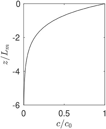
Figure 1. Depth profile of normalized concentration of buoyant particles c/c₀ as a function of z/L_m according to the wind-mixing model as described by Equation (2).

One common use of this model is to extrapolate surface measurements to total water column concentrations (e.g., Cozar et al., 2014; Kooi et al., 2016; Lebreton et al., 2018; Poulain et al., 2019). This extrapolation can be done by reconfiguring the model as a correction factor f defined as

$\begin{array}{ll}f=\frac{N}{N_{tow}}=\frac{{\displaystyle {\int }_{-\infty }^0}c(z)dz}{{\displaystyle {\int }_{z_0}^0}c(z)dz}=\frac{1}{1-exp(z_0/L_m)},& (3)\end{array}$

where N is the predicted total count of microplastics in the water column, and N_tow is the number of microplastics captured in the towed net (Kukulka et al., 2012). The parameter z₀ represents the depth over which plastic was measured, or the average submergence of the towed net.

3. Methods

The wind-mixing model is the current standard used to correct surface microplastic measurements, so we start with the assumptions within this model to examine the effects of surface gravity waves. This model includes only uniform turbulence and particle buoyancy. The assumption of constant eddy viscosity is only valid very close to the surface.

In addition, this model assumes that particle inertia effects are negligible. The relative importance of particle inertia can be defined by the particle's Stokes number St, which is a ratio between the particle relaxation timescale and the relevant flow timescale. A small Stokes number implies that the particle behaves as a flow tracer with little to no particle inertia effects. In this case, we assume the particle relaxation time τ_p is defined as τ_p = w_p/g, and the relevant flow time scales are the wave period T and the Kolmogorov timescale of the turbulence τ_η. Thus, we can construct a wave Stokes number St_w and a turbulence Stokes number St_η. A common measured rise velocity for microplastics is w_p = 1 cm/s (Kukulka et al., 2012), which corresponds to buoyant microplastics of about 1 cm according to Figure 2 in Poulain et al. (2019). Using τ_p = w_p/g, we find τ_p ≈ 0.001 s. Wind wave periods are on the order of seconds, so $S{t}_w={O}(10^{-3})\ll 1$ and the assumption of no particle inertia is valid. In terms of the turbulence, a conservative estimate using a high dissipation rate at the ocean surface boundary layer of 10⁻³ m²/s³ corresponds to τ_η ≈ 0.03 s (Zippel et al., 2018). In this case, $S{t}_{\eta }={O}(10^{-2})\ll 1$ as well. While the assumption of negligible particle inertia theoretically holds in this case for microplastic particles up to approximately 1 cm, finite-size effects may be important for particles at this size and should be studied further.

In order to isolate the wave effects, we consider a progressive train of surface gravity waves in deep-water. We start with linear wave theory which assumes that the wave-induced flow is irrotational, incompressible, and 2-dimensional. It also assumes small amplitude waves with a free surface deflection η, where η = Acosθ and θ = kx − ωt is the wave phase. In this system t represents time, x is the horizontal coordinate, and z is the vertical coordinate where z = 0 is the free surface. We further assume that the waves are traveling over an infinite depth H such that kH ≫ 1, referred to as the deep-water wave limit. The waves are controlled by the wave number k, related to the wave length λ where k = 2π/λ; the wave frequency ω, related to the wave period T where ω = 2π/T; and the wave amplitude A. These parameters are not independent as the deep-water dispersion relationship states $\omega =\sqrt{gk}$ where g is the acceleration due to gravity. We will refer to the vertical coordinate relative to the instantaneous free surface as ζ = z − η. A schematic of the wave's geometry, its induced velocity field, and the coordinate system is shown in Figure 2.

FIGURE 2

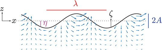
Figure 2. Example of the wave geometry and the wave induced velocity field shown as scaled vectors. The wave is traveling in the postive x direction, with wavelength λ and wave amplitude A. The free surface is denoted by η, and ζ is the coordinate representing distance from the instantaneous free surface.

In this model, without waves, the particles are mixed solely due to turbulence and vertically transported due to buoyancy, and the only length scale in the problem is the mixing scale L_m. With the addition of waves, new length scales are introduced. The waves are controlled by ϵ = kA which is the relative wave steepness. Linear wave theory assumes ϵ≪1, and physically ϵ < 0.44 or the waves will break (Stokes, 1880; Perlin et al., 2013). To relate the mixing to the waves, we use the ratios A/L_m and kL_m.

The exact values of A/L_m and ϵ in the ocean will vary considerably. Kukulka et al. (2012) considered a range of L_m from about 0.4–4 m. The most extreme sea state that samples are conducted under is Beaufort 5 which can have wave amplitudes on the order of 1.5 m. Therefore, we report findings using A/L_m values of 1/3, 1, and 3 across a range of ϵ from 0 to 0.4 to demonstrate the variability of scenarios potentially encountered during sampling.

3.1. Analytical Model

3.1.1. Wave-Averaged Distribution

Surface gravity waves induce wave-orbital motions and deflect the free surface, both of which can affect buoyant particle distributions. We first address the distortion of the free surface; we model this effect by considering a superposition of the wind-mixing model shifted to the instantaneous free surface and averaged over a wave period. We assume a linear wave η = Acosθ, and we denote the phase-dependent concentration as $\tilde{c}$, where in this case

$\begin{array}{ll}\tilde{c}\left(\theta ,z\right)=\{\begin{array}{cc}{c}_{0}exp\left(\frac{z-\eta \left(\theta \right)}{L_m}\right)\hfill & z\le \eta \left(\theta \right)\hfill \\ 0\hfill & z>\eta \left(\theta \right).\hfill \end{array}\hfill & (4)\end{array}$

We average this concentration over a wave-period, where $\overline{\tilde{c}}$ is a wave-period averaged quantity,

$\begin{array}{ll}\overline{\tilde{c}}(z)=\frac{1}{2\pi }{\displaystyle {\int }_0^{2\pi }}\tilde{c}(\theta ,z)\text{d}\theta .& (5)\end{array}$

This expression is evaluated exactly for all points under the wave trough, and above the wave trough the integration range is a function of z/A, which can be integrated numerically. The full expression is:

$\begin{array}{ll}\overline{\tilde{c}}\left(z\right)=\{\begin{array}{cc}c\left(z\right)I_0\left(\frac{A}{L_m}\right)\hfill & z\le -A\hfill \\ c\left(z\right)\frac{1}{2\pi }{\displaystyle {\int }_{co{s}^{-1}\left(-z/A\right)}^{2\pi -co{s}^{-1}\left(-z/A\right)}}exp\left(-\frac{A}{L_m}cos\theta \right)d\theta -A<\hfill & z<A\hfill \end{array}\hfill & (6)\end{array}$

where I₀ is an elliptic integral of the first kind. From inspection, we see that the wave-averaged vertical distribution $\overline{\tilde{c}}(z)$ is a function of the original solution without waves, c(z), and a factor dependent on the ratio A/L_m. As A/L_m → 0, the wave solution approaches the no-wave solution, or $\overline{\tilde{c}}(z)\to c(z)$.

3.1.2. Wave-Phase Variability

Waves also alter the vertical and horizontal particle distributions as a function of wave phase. These effects are largely due to the wave-orbital motion of the particles. We begin our analysis with a study of how the wave kinematics affect the horizontal distribution of particles. At one point in time, horizontal position maps onto wave phase. Thus, we use wave phase distribution as a proxy for the horizontal distribution. We approximate wave phase as a function of time by linearizing the particle equations of motion. Under linear wave theory in deep-water, the horizontal and vertical wave-orbital velocities, respectively, are:

$\begin{array}{ll}{u}_w=A\omega {\text{e}}^{kz}cos\theta & (\mathrm{7a})\end{array}$

$\begin{array}{ll}{w}_w=A\omega {\text{e}}^{kz}sin\theta .& (\mathrm{7b})\end{array}$

Next, we approximate the horizontal particle motion as ξ where $\stackrel{\bullet }{\xi }=u_w(x_0,z,t)$, and x₀ is a constant value that refers to the center of the particle's horizontal motion. By integration, ξ(t) = − Aexpkzsin(kx₀ − ωt). Assuming x ≈ ξ(t), we plug this into our expression for θ(t) leaving:

$\begin{array}{ll}\theta (t)\approx -ϵ{\text{e}}^{kz}sin(k{x}_0-\omega t)-\omega t.& (8)\end{array}$

To obtain the probability distribution function (p.d.f.) of θ over t, we use a Jacobian transformation where p(θ) = |dt/dθ|p(t) for a uniform probability of t over one wave period. We then further approximate θ ≈ kx₀ − ωt to obtain a closed form solution. At this level of approximation, we find the p.d.f. of θ given a value of z to be

$\begin{array}{ll}p\left(\theta \mid z\right)=\frac{1}{2\pi }{\left(1-ϵ{\text{e}}^{kz}cos\left(\theta \right)\right)}^{-1}.& (9)\end{array}$

We account for the phase variations over the vertical distribution of particles by weighting Equation 9 with the no-wave vertical particle distribution from Equation (2), vertically integrating from z = − ∞ to z = 0, and normalizing the resultant equation:

$\begin{array}{ll}p(\theta )=\frac{1}{L_{m}2\pi }{\displaystyle {\int }_{-\infty }^0}\frac{{\text{e}}^{z/L_m}}{ϵ{\text{e}}^{kz}cos(\theta )-1}dz.& (10)\end{array}$

This integration is solved numerically to find the vertically-averaged wave-phase p.d.f. of buoyant particles. Note that the p.d.f. of particles over wave phase is controlled by the parameters k, L_m and ϵ. For large kL_m or small ϵ, the p.d.f. becomes uniform over a wave.

While Equation 10 describes how waves affect the total amount of particles under each wave phase, we also find that waves can change the shape of the distributions under a wave. They do this through vertical stretching and compression which has been studied previously in relation to vortical structures and turbulence (Phillips, 1961; Guo and Shen, 2013). The stretching of the distribution is controlled by the vertical divergence of the flow: dw/dz = ωϵexpkzsinθ. To quantify these effects, we calculate L_m as a function of wave phase and account for the vertical stretching with the following relationship, approximating the stretching effect by integrating in time:

$\begin{array}{ll}\widetilde{L_m}\left(\theta \right)=\left(1+{\displaystyle \int }\frac{dw}{dz}dt\right)L_m& (11)\end{array}$

After integrating and evaluating at z = η − L_m, we are left with

$\begin{array}{ll}\widetilde{L_m}(\theta )=(1+ϵ{\text{e}}^{ϵcos\theta -k{L}_m}cos\theta )L_m.& (12)\end{array}$

In this case, $\widetilde{L_m}$ is measured from the instantaneous free surface. The waves' effects on L_m are strongest for large ϵ and small kL_m.

We synthesize our results from Equations (10) and (12) and find an expression for the vertical distribution of particles under waves and turbulence:

$\begin{array}{ll}\frac{\tilde{c}(\theta ,\zeta )}{c_0}=p(\theta )exp(\zeta /\widetilde{L_m}(\theta ))\mid \zeta \le 0& (13)\end{array}$

This equation is similar to Equation (4), but it now accounts both for the wave-orbital motion effects as well as the effects of the unsteady free surface. It is also a function of ζ, which is the vertical coordinate relative to the instantaneous free surface. In order to both validate this model and expand on its theory, we also conducted complementary numerical simulations.

3.2. Numerical Simulations

To complement the analytical model, we use simple numerical simulations with Lagrangian particle tracking. The turbulent dispersion is modeled using a random walk, which allows us to track individual particles. These Lagrangian simulations contrast the Eulerian analytical model of the concentration field. They also allow for a more accurate representation of the wave field without the approximations made in the derivations.

In the simulations, the wave field is imposed using the analytical form of Stokes third order deep-water waves. Because we are interested in particle behavior near the free surface, we use Stokes third order waves to minimize the errors between the trajectories of particles at the free surface, and the free surface itself. This error is ${O}({\epsilon }^2)$ for linear wave theory, but ${O}({\epsilon }^4)$ for Stokes waves. At this level of approximation, the free surface η is defined as

$\begin{array}{ll}\eta =A\left({\displaystyle [}1-\frac{1}{16}{ϵ}^2{\displaystyle ]}cos\theta +\frac{1}{2}ϵcos2\theta +\frac{3}{8}{ϵ}^{2}cos3\theta \right),& (14)\end{array}$

with wave phase θ = kx − ω′t where ${\omega }^{\prime }=(1+\frac{1}{2}{ϵ}^2)\omega$. The wave-induced velocity field described in Equation (7) is extrapolated to the wave crests due to the agreement seen in Baldock et al. (1996) and as summarized in Smit et al. (2017).

The particle trajectories are simulated using a fourth order Runge Kutta integration which calculates particle velocity based on the superposition of the analytical wave velocity field (see Equation 7) and a constant rise velocity w_p. After the velocity is calculated, a random walk perturbation in the vertical and horizontal directions is applied based on the time-step Δt and κ_t:

$\begin{array}{ll}\frac{d{x}_p}{dt}=u_w(x,z,t)+\frac{X\sqrt{2{\kappa }_t\Delta t}}{\Delta t},& (\mathrm{15a})\end{array}$

$\begin{array}{ll}\frac{d{z}_p}{dt}=w_w(x,z,t)+\frac{Y\sqrt{2{\kappa }_t\Delta t}}{\Delta t}+w_p,& (\mathrm{15b})\end{array}$

with normally distributed random variables X, Y $~{N}(0,1)$. Particles were constrained to not go above the free surface by setting z = η for all particles with z > η after each integration step using Equation (14).

The ratio A/L_m and ϵ were varied for a total of 42 unique scenarios. The values of A/L_m were varied from 1/10 to 10, and the values of ϵ were varied from 0 to 0.3. Due to similarities among the trials, we only report results from a subset of the runs.

The simulations were run in MATLAB and started with 1,000 particles at the surface distributed evenly over one wave period, defined by the range {x ∣ 0 ≤ x ≤ 2π/k}, and run until the vertical distribution and wave phase distribution reached equilibrium. Once at equilibrium, the simulations were run for at least an additional 1,000 wave cycles, at which point the data was sampled periodically resulting in 1,000,000 data points for each run.

4. Model Results

Both the numerical simulations and the analytical model demonstrate how the unsteady free surface associated with surface gravity waves fundamentally alters the equilibrium vertical and horizontal distributions of buoyant particles. This can be seen in Figure 3, where we plot $\overline{\tilde{c}}(z)$, the wave-period averaged concentration in the fixed coordinate system for different A/L_m values from both the numerical simulations and the analytical model. For each case, the peak concentration is at the level of the wave trough (when z/L_m = − A/L_m), and below this depth the distribution resembles an exponentially decaying curve. However, above this depth, the distribution deviates from the exponential curve. This is due to the fact that there is an unsteady free surface wetting and drying, and thus there are fewer total particles on average when compared to the case without waves. As A/L_m increases, the distribution above the trough level becomes more uniform, and as A/L_m decreases, the distribution approaches the case without waves.

FIGURE 3

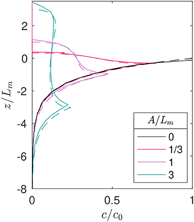
Figure 3. Wave-averaged concentration of particles over the water column. The ratio A/L_m was varied with constant ϵ = 0.15. The solid lines denote the results from numerical simulations, and the dashed lines denote Equation (6).

The wave-orbital motion of the particles also introduces phase variation in the distributions. In Figure 4 we plot the phase-averaged p.d.f. of particles from both the numerical simulations and the theory using Equation 10. In this figure, we see that on average, particle concentration is enhanced under the wave crests (θ = 0, 2π) and reduced below the troughs (θ = π). For the steepest waves, the number of particles under the wave crest can be up to 50% larger than under the wave trough.

FIGURE 4

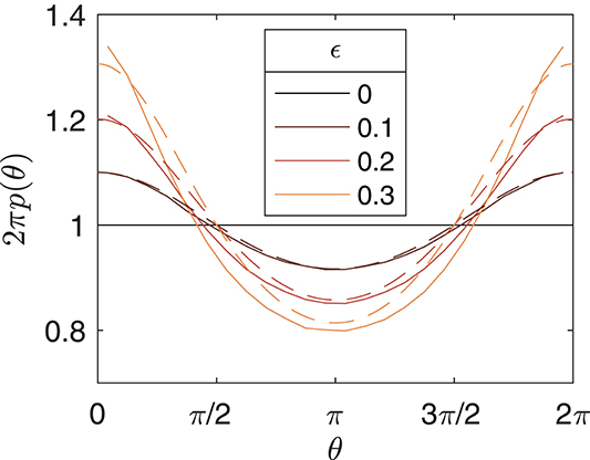
Figure 4. Normalized probability density function 2πp(θ) of particles in the water column as a function of wave phase. The ratio A/L_m = 1 and ϵ is varied from 0 (no waves) to 0.3. The solid line shows results calculated from numerical simulations and the dashed line shows Equation (10).

The total concentration of particles is phase-dependent, and so is the shape of their vertical distribution. In Figure 5, we plot the concentration of particles over depth, relative to the instantaneous free surface. The data are from numerical simulations with ϵ = 0.2 and A/L_m = 3, and are subdivided into the concentration under the wave trough, wave crest, the average profile over the wave, and the no-waves case for reference. As expected, the wave crest has higher concentrations than the wave trough. The largest difference in concentrations is near the surface, and the concentration profiles approach each other at depth. The surface concentration at the crest can be up to 50% larger than the average surface concentration across the wave. We also see that the average vertical profile, when adjusted to the instantaneous free surface, recovers a similar profile to the no-wave case.

FIGURE 5

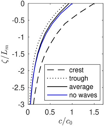
Figure 5. Vertical distribution of relative concentration of buoyant particles under waves as a function of wave phase from numerical simulations. Data comes from a simulation with A/L_m = 3 and ϵ = 0.2. The wave phase was subdivided where the crest is the region defined by θ < 0.04 π or θ > 2 π − 0.04 π and the trough is defined by π − 0.04 π < θ < π + 0.04π. The no waves line shows the distribution from Equation (2), and the average line shows the wave-period averaged distribution.

Another way to visualize the phase-dependence of the particle distributions is with a 2-dimensional p.d.f. of particles over wave-phase and relative depth as plotted in Figure 6. In this figure, we again see that the peak concentration at the surface is largest under the wave crests. To characterize the shape of the distribution, we calculate the exponential decay length scale, or mixing length scale $\widetilde{L_m}$, which is plotted as a solid line from the numerical simulations and a dashed line using Equation (12). The two solutions agree with each other. The value of $\widetilde{L_m}$ is smaller under the troughs than it is under the crests, indicating that the vertical distribution is compressed under the troughs and stretched under the crests.

FIGURE 6

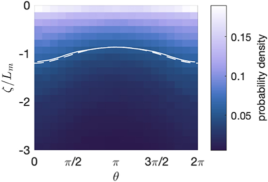
Figure 6. Two-dimensional probability density function of $\tilde{c}(\theta ,\zeta )$ for ϵ = 0.2 and A/L_m = 1. The solid line shows the effective $\widetilde{L_m}(\theta )$ calculated from the numerical simulations, and the dashed line shows $\widetilde{L_m}(\theta )$ calculated from Equation (12).

The results from both the analytical model and the numerical simulations demonstrate that waves can affect the distribution of buoyant particles near the free surface. The benefit of the numerical simulations is that they are more accurate, however they have a higher computational cost associated with them. Nevertheless, the numerical simulation results largely agree with the theory described in section 3.1, but they differ in a few distinct ways. The waves considered in the theory are from linear wave theory, but the numerical simulations use higher order harmonics. These non-linear wave effects result in waves with taller crests and shallower troughs, the effects of which can be seen in Figure 3 where the microplastics reach higher in the water column in the numerical simulations when compared with the analytical model. The surface boundary condition combined with the discrete random walk used in the simulations also results in a concentration discontinuity at the free surface; this is a small effect only seen when analyzing the results very close to the free surface, which is done in the following section. However, the close agreement between the two methods show that the assumptions behind our analytical model capture the major effects of waves in these scenarios.

5. Sampling Implications

In this section we consider how the waves may affect the sampling of microplastics at the ocean surface. Under the wind-mixing model, a constant free surface profile at z = 0 is assumed. If the free surface is deflected due to waves, the total surface area between two fixed points increases. A net trawled over a wavy free surface will not sample around z = 0, but rather around z = η. The waves may also cause the net to sample less effectively; if the net lags the waves, it will not exactly track the free surface with a constant sample volume and the assumption of a single z₀ value may break down. We consider how these effects may alter the particles sampled under various scenarios.

If we let δ be the submerged height of the net opening (where δ corresponds to a varying z₀), W be the width of the net opening, and d be the distance the net traveled over the free surface, then the total sampled volume of water is V = dδW. Let the total number of particles counted in the net be N_tow. Thus, the measured concentration is c_tow = N_tow/V. While W should be constant, d is a function of the free surface deflection, and δ can vary due to the net moving relative to the water surface. We apply this framework to our wave-phase distribution results to discern the possible effects of waves on sampling.

5.1. Surface Tow Length

A net following a deflected free surface will sample a larger volume than if trawled over a flat free surface. The total distance trawled is a function of the free surface deflections, where d from x = x_a to x = x_b is defined using the arc-length formula as

$\begin{array}{ll}d={\displaystyle {\int }_{x_a}^{x_b}}\sqrt{1+{\frac{d\eta }{dx}}^2}dx.& (16)\end{array}$

Over one wave length λ, we integrate Equation (16) for a linear wave which results in an expression using an elliptic integral of the second kind E(m):

$\begin{array}{ll}d={\displaystyle {\int }_0^{2\pi /k}}\sqrt{1+{\left(ϵsinkx\right)}^2}dx=\frac{4}{k}\sqrt{1+{ϵ}^2}E\left(\frac{{ϵ}^2}{1+{ϵ}^2}\right).& (17)\end{array}$

The effective increase in the length of free surface due to the wave can be defined by the ratio d/λ which is only a function of the wave steepness ϵ:

$\begin{array}{ll}\frac{d}{\lambda }=\frac{2}{\pi }\sqrt{1+{ϵ}^2}E\left(\frac{{ϵ}^2}{1+{ϵ}^2}\right).& (18)\end{array}$

For a very steep wave where ϵ = 0.3, we find d/λ = 1.022 for a linear wave and 1.024 for a 3rd order Stokes wave. These are small differences in total tow length that are not necessarily larger than other sources of error during the sampling processes. However, this analysis assumes that as the sample volume travels one linear distance λ, it samples exactly one wave. In reality, the sample volume and the wave are both traveling. Under a traveling wave, d is a function of the relative speed between the sampler and the wave. For simplicity, we will assume that the wave and the sampler are traveling in the same plane. (This is often the case, as sampling vessels will align into the wind direction in order to minimize net destabilization from cross-winds.) If the sampler travels at speed U, then the free surface at the sampler as a function of time is

$\begin{array}{ll}\eta =Acos\left(\left[kU-\omega \right]t\right).& (19)\end{array}$

This relationship yields a new effective wave steepness ϵ′:

$\begin{array}{ll}{ϵ}^{\prime }=\left(k-\frac{\omega }{U}\right)A=ϵ\left(1-\frac{c_p}{U}\right),& (20)\end{array}$

where c_p = ω/k is the wave phase speed. Larger values of ϵ result in larger values of d/λ. Thus, the expression for ϵ′ suggests that the effective wave steepness is very sensitive to the relative speed of the boat and the waves. Even moderate waves traveling against the direction of the boat can dramatically increase the effective surface area trawled. For example, a boat traveling at 2 knots in the opposite direction of a 50 cm, 5 s deep-water wave where ϵ = 0.08 has ϵ′ = 0.69 and d/λ = 1.11.

The wave-enhanced tow length effect is relevant to the way in which concentrations are calculated from net trawls. The volume of water sampled is sometimes measured directly using a flow meter attached to the net (Isobe et al., 2014; Kooi et al., 2016), but it can also be estimated by using the linear distance of the trawl (often calculated using GPS coordinates) (Law, 2010; Lebreton et al., 2018). The former method may better capture the free surface deflections due to waves as compared to the latter. Let the concentration calculated using the total arc-length of the free surface be c_tow, and $c_{tow}^0$ be the concentration calculated using only the linear distance traveled. To assess the sensitivity of these two concentration measurement techniques to waves, $c_{tow}/c_{tow}^0$ is plotted in Figure 7 as a function of c_p/U and ϵ. In this case, $c_{tow}/c_{tow}^0=\lambda /d$ assuming constant N_tow, δ, and W values. As seen in the figure, waves can reduce the measured concentration by up to 50% in the most extreme cases. This difference could potentially account for some of the discrepancies across different measurement techniques in wavy conditions.

FIGURE 7

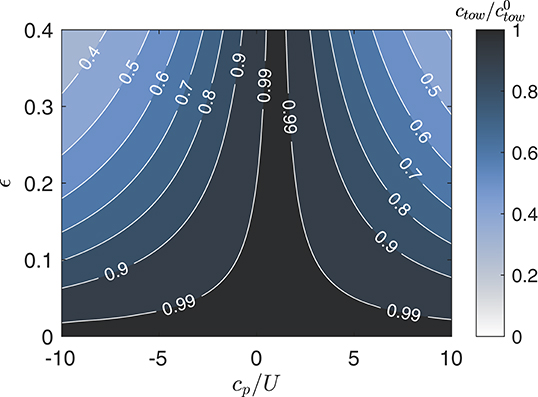
Figure 7. Contour plot of relative concentration calculated using total arc length in waves vs. no waves $c_{tow}/c_{tow}^0$, plotted as a function of wave steepness ϵ and relative wave speed c_p/U. The values were calculated using Equations (18) and (19).

5.2. Non-uniform Sampling Effects

The ideal trawling scenario has a net that samples at a constant depth below the free surface. If the free surface is unsteady, then the depth of the trawl relative to mean water level is η − δ. In many cases, the net does not necessarily sample at a constant depth. We consider the effects of non-uniform net sampling by assuming that the net lags the free surface resulting in an oscillation with a smaller amplitude:

$\begin{array}{ll}\delta (t)=(1-\alpha )\eta +\overline{\delta },& (21)\end{array}$

where α is the amplitude reduction factor. Ideal sampling results in a constant δ value with α = 1. A sampler that never moves vertically and constantly samples around z = 0 corresponds to α = 0. The sample volume over a wave as a function of α is shown schematically in Figure 8. To assess the effects for α≠1, we also assume that the net never leaves the water surface such that $\overline{\delta }>(1-\alpha )A$. Finally, we only consider α ≤ 1 where the troughs are sampled less than the crests. We argue that this corresponds to the more relevant scenario where the net lags the free surface, rather than leads it.

FIGURE 8

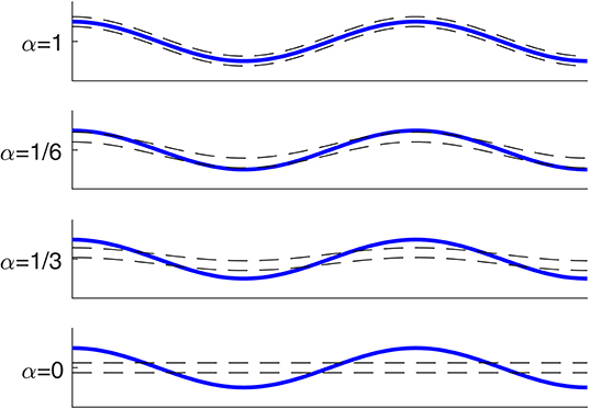
Figure 8. Schematic showing the virtual net sampling volume δ over a wave for different α values as described by Equation (21). The net sampling volume is denoted by the area between the two black dashed lines, and the free surface is shown with the solid blue line. In this case, $\overline{\delta }/A=0.2$. The wave-averaged sampled volume is constant for all α.

We apply Equation (21) to the numerical simulation results and the distribution modeled by Equation 13 to evaluate how a non-uniform sampler affects the measured number of particles. We assume the net is twice the height of $\overline{\delta }$; this means on-average the net is halfway submerged. Over a wave cycle, the particles above δ and below the top of the net are integrated to determine the effective N_tow. The value N_tow is then normalized by the reference $N_{tow}^0$ which is calculated using Equation (3). The value of $N_{tow}^0$ represents the number of measured particles using the wind-mixing model with no waves. Assuming a constant volume sampled in both scenarios, the resultant $c_{tow}/c_{tow}^0$ values are plotted against α for various wave scenarios in Figure 9. We also consider two different net sizes by varying the ratio $\overline{\delta }/A$.

FIGURE 9

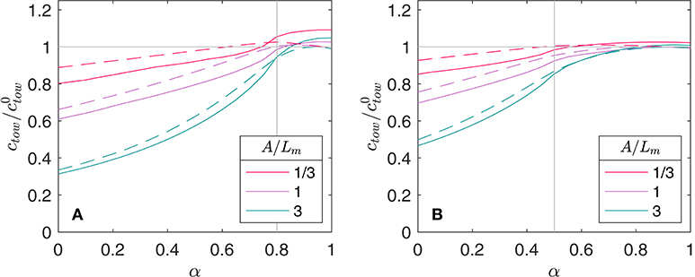
Figure 9. Modeled captured particles as a function of net lag parameter α for various A/L_m. The total number of particles captured in a net tow per volume c_tow is normalized by $c_{tow}^0$ which represents the predicted amount without waves. The solid lines denote the results from numerical simulations, and the dashed line denote the results using the analytically modeled concentration as described by Equation (13). The vertical gray line denotes the α value when the net drops below the free surface for part of the wave cycle. In these data, ϵ = 0.1 in both cases, and $\overline{\delta }/A=0.2$ (A) and $\overline{\delta }/A=0.5$ (B).

In Figure 9, we see that as α decreases, the amount of particles sampled decreases relative to the no-wave prediction. The effect is the strongest for large A/L_m. The concentrations show the most decrease after the net starts to dip below the free surface for part of the wave cycle, denoted by the vertical lines. In Figure 9A, $\overline{\delta }/A=0.2$, and in Figure 9B, $\overline{\delta }/A=0.5$; by comparing these figures we see that the larger the net is relative to the wave amplitude, the less sensitivity there is to α. However, once the net goes under water in both scenarios, we see a decrease in sampled concentrations. An increase in c_tow/$c_{tow}^0$ is seen in the numerical simulations for α values close to 1 in Figure 9A. This is due to a slight enhancement of particles at the free surface in the simulations as a result of the surface boundary condition.

6. Discussion

Using a phase-resolving approach, we have analyzed the effects of waves on the equilibrium distribution of buoyant particles in the ocean mixed layer, demonstrating that waves introduce concentration differences across a wave cycle. This work implies that if a towed net does not sample each wave phase equally, the resulting observations will be biased.

The phase variability in the distributions is controlled by the wave kinematics. A tracer particle under a linear wave field spends more time under the crests than the trough. One way to conceptualize this phenomena is by considering a particle traveling under a trough and under a crest. The particle under the trough moves in the opposite direction of the wave, so it is leaving the trough more quickly than if the wave was not traveling. However, under the wave crest, the particle is moving in the direction of the wave, so it has a longer residence time in its relative wave phase. In other words, dθ/dt has a higher magnitude under the troughs than under the crests. This translates to particles on-average, non-uniformly distributed in wave-phase, with more particles under the crests than the troughs.

Another major focus of this study is how waves stretch and compress the particle distributions as a function of wave phase. While these processes have been studied in relation to turbulence and vortices, this work centers on particle distributions. The wave-induced velocities have non-zero vertical divergence. This results in the distribution of particles being maximally stretched under the crests, i.e., having the maximum $\widetilde{L_m}$ value, and being maximally compressed under the troughs, i.e., having the minimum $\widetilde{L_m}$ value. Because the time-averaged vertical divergence in the wave field is zero, there is no net effect, and this stretching is only seen as a function of wave phase. These findings demonstrate that particles are distributed the deepest relative to the free surface under the crests, whereas they are closest to the surface under the troughs. This result is illustrated in Figure 6.

Because particles preferentially accumulate under the crests relative to the troughs, if a towed net over-samples the wave crests, it can over-sample the particles. However if the net tends to go under water at the crests, it can under-sample the particles because it will miss the peak concentration at the surface. Another common assumption during net tow sampling is that a net that is on-average halfway submerged will sample the same particles as a net that has constant halfway submergence. A net that comes out of water half the time and submerges underwater half the time, is on-average halfway submerged and corresponds to small α values; we have shown that small α values consistently lead to the under-sampling of particles. Therefore, if waves cause the towed net's submergence to vary over time, under-sampling can result. These effects should be studied more carefully during the time of sampling to further discern any bias in the measurements.

One can imagine there is a range of frequencies to which the sampling net can respond. At the low frequency limit for long waves, i.e., waves which are much longer than the net, the net should be able to effectively track the free surface. In that case, the wind-mixing model is still an appropriate measure to use. However, if the net tends to sample at a constant z-level and move through the waves, which may occur with short-period waves, i.e., waves with higher frequencies than the net's natural response frequency, then the modified wave-period-averaged wind-mixing model presented here may be more appropriate. In that scenario, the net will also under-sample the assumed concentration estimated by the wind-mixing model as seen in Figure 3.

When compared to other sampling methods, there is some evidence that net tows can under-sample. For example, grab samples of microplastics measurements have been reported with high values relative to the net tows at the same location (Barrows et al., 2017). This effect is also due to the ability for grab samples to capture particles smaller than the net's mesh size. However, this does not necessarily explain all the discrepancy in observed concentrations, and non-uniform sampling due to waves could be partly responsible. An advantage of net tows in this scenario is that they encompass average concentrations over large distances which lowers sensitivity and variability to patchiness, whereas grab samples are very sensitive to patchiness. Microplastics patchiness can occur due to Langmuir circulation and other hydrodynamic features (van Sebille et al., 2020).

We find that the accumulation of particles under the wave crests is most extreme under the steepest waves. Therefore, as waves steepen before they break, they will accumulate particles under them. The turbulence due to breaking waves is also strongest under the crests of waves (Rapp and Melville, 1990), and thus enhanced turbulent mixing will occur at the point with the highest concentration of particles at the time of breaking. This coupling could result in greater transport of particles away from the surface and should be studied further.

The ocean surface boundary layer is subjected to a multitude of unsteady forcings. Understanding how they each can bias measurements is important to accurately interpreting data, and this study represents only one mechanism: non-breaking surface gravity waves. In this work, we have only considered a monochromatic wave train aligned with the sampler, and therefore future work should include a wave field with a broadband spectrum as well as scenarios in which waves travel obliquely to the sampling apparatus. We have also neglected the effects of Langmuir turbulence, which has been shown to be extremely important in both controlling patchiness and transporting particles to depth. Finally, understanding the limits of the wind-mixing model is important. When L_m is greater than the mixed layer depth, the model's underlying assumption of a constant eddy viscosity no longer holds (Kukulka et al., 2012). Large L_m values can result from small particle rise velocities, and thus this model may not be appropriate for the smallest microplastic particles. A more general model that can account for the smallest particles as well as the effects of waves is therefore needed.

7. Conclusions

Using both numerical simulations and an analytical model, we have demonstrated how waves affect the vertical and horizontal distributions of buoyant particles at the free surface. In the fixed frame, waves change the wave-period-averaged vertical distribution of particles by lowering the peak concentration of particles to the level of the wave trough. Over a wave cycle, the wave orbital motion redistributes the particles so that on average, more particles are under the wave crest than under the wave trough. Waves also stretch the vertical distribution resulting in a smaller mixing length under the wave trough and a larger mixing length under the wave crest. The free surface is stretched due to waves, and when a sampling volume is traveling relative to the waves, the effective length of the trawl can increase dramatically. Finally, we find that non-uniform sampling of a wave can result in reduced measured particle concentrations relative to predictions based on the wind-mixing model (Kukulka et al., 2012).

While we have shown how a train of monochromatic progressive waves distort buoyant particle distributions, the real ocean surface is subjected to a spectrum of waves. The turbulent mixing at the ocean surface is not necessarily constant nor isotropic. It is also not independent from the waves. Particle inertia can also be important for large particles and low turbulence forcing. However, this work shows the possible range of effects of surface gravity waves on buoyant particle distributions. We recommend a more detailed study of how the trawling process can bias the concentrations observed, and how our findings change under more complicated scenarios.

Data Availability Statement

The datasets generated for this study are available on request to the corresponding author.

Author Contributions

MD conceived and designed the study, developed and analyzed the models, interpreted results, and wrote the manuscript.

Funding

This work was supported by the Postdoctoral Scholar Program at the Woods Hole Oceanographic Institution, and by the US National Science Foundation under grant no. CBET-1706586.

Conflict of Interest

The author declares that the research was conducted in the absence of any commercial or financial relationships that could be construed as a potential conflict of interest.

Acknowledgments

The author would like to acknowledge Nicholas T. Ouellette and Jeffery R. Koseff for helpful discussions and support over the course of this work.

References

Babanin, A. V. (2006). On a wave-induced turbulence and a wave-mixed upper ocean layer. Geophys. Res. Lett. 33, 1–6. doi: 10.1029/2006GL027308

CrossRef Full Text | Google Scholar

Baldock, T. E., Swan, C., and Taylor, P. H. (1996). A laboratory study of nonlinear surface waves on water. Philos. Trans. R. Soc. A Math. Phys. Eng. Sci. 354, 649–676. doi: 10.1098/rsta.1996.0022

CrossRef Full Text | Google Scholar

Barrows, A. P., Neumann, C. A., Berger, M. L., and Shaw, S. D. (2017). Grab: vs. neuston tow net: a microplastic sampling performance comparison and possible advances in the field. Anal. Methods 9, 1446–1453. doi: 10.1039/C6AY02387H

CrossRef Full Text | Google Scholar

Boufadel, M. C., Bechtel, R. D., and Weaver, J. (2006). The movement of oil under non-breaking waves. Mar. Pollut. Bull. 52, 1056–1065. doi: 10.1016/j.marpolbul.2006.01.012

PubMed Abstract | CrossRef Full Text | Google Scholar

Brunner, K., Kukulka, T., Proskurowski, G., and Law, K. L. (2015). Passive buoyant tracers in the ocean surface boundary layer: 2. Observations and simulations of microplastic marine debris. J. Geophys. Res. Oceans 120, 7559–7573. doi: 10.1002/2015JC010840

CrossRef Full Text | Google Scholar

Chamecki, M., Chor, T., Yang, D., and Meneveau, C. (2019). Material transport in the ocean mixed layer: recent developments enabled by large eddy simulations. Rev. Geophys. 57, 1338–1371. doi: 10.1029/2019RG000655

CrossRef Full Text | Google Scholar

Cozar, A., Echevarria, F., Gonzalez-Gordillo, J. I., Irigoien, X., Ubeda, B., Hernandez-Leon, S., et al. (2014). Plastic debris in the open ocean. Proc. Natl. Acad. Sci. U.S.A. 111, 10239–10244. doi: 10.1073/pnas.1314705111

PubMed Abstract | CrossRef Full Text | Google Scholar

DiBenedetto, M. H., Ouellette, N. T., and Koseff, J. R. (2018). Transport of anisotropic particles under waves. J. Fluid Mech. 837, 320–340. doi: 10.1017/jfm.2017.853

CrossRef Full Text | Google Scholar

Eames, I. (2008). Settling of particles beneath water waves. J. Phys. Oceanogr. 38, 2846–2853. doi: 10.1175/2008JPO3793.1

CrossRef Full Text | Google Scholar

Eriksen, M., Lebreton, L. C., Carson, H. S., Thiel, M., Moore, C. J., Borerro, J. C., et al. (2014). Plastic pollution in the world's oceans: more than 5 trillion plastic pieces weighing over 250,000 tons afloat at sea. PLoS ONE 9:e111913. doi: 10.1371/journal.pone.0111913

PubMed Abstract | CrossRef Full Text | Google Scholar

Geyer, R., Jambeck, J. R., and Law, K. L. (2017). Production, uses, and fate of all plastics ever made. Sci. Adv. 3:5. doi: 10.1126/sciadv.1700782

CrossRef Full Text

Guo, X., and Shen, L. (2013). Numerical study of the effect of surface waves on turbulence underneath. Part 1. Mean flow and turbulence vorticity. J. Fluid Mech. 733, 558–587. doi: 10.1017/jfm.2013.451

CrossRef Full Text | Google Scholar

Herterich, K., and Hasselmann, K. (1982). The horizontal diffusion of tracers by surface waves. J. Phys. Oceanogr. 12, 704–711. doi: 10.1175/1520-0485(1982)012<0704:THDOTB>2.0.CO;2

CrossRef Full Text | Google Scholar

Hidalgo-Ruz, V., Gutow, L., Thompson, R. C., and Thiel, M. (2012). Microplastics in the marine environment: a review of the methods used for identification and quantification. Environ. Sci. Technol. 46, 3060–3075. doi: 10.1021/es2031505

PubMed Abstract | CrossRef Full Text | Google Scholar

Isobe, A., Kubo, K., Tamura, Y., Kako, S., Nakashima, E., and Fujii, N. (2014). Selective transport of microplastics and mesoplastics by drifting in coastal waters. Mar. Pollut. Bull. 89, 324–330. doi: 10.1016/j.marpolbul.2014.09.041

PubMed Abstract | CrossRef Full Text | Google Scholar

Jambeck, J. R., Geyer, R., Wilcox, C., Siegler, T. R., Perryman, M., Andrady, A., et al. (2015). Plastic waste inputs from land into the ocean. Science 347, 768–771. doi: 10.1126/science.1260352

PubMed Abstract | CrossRef Full Text | Google Scholar

Karlsson, T. M., Kärrman, A., Rotander, A., and Hassellöv, M. (2019). Comparison between manta trawl and in situ pump filtration methods, and guidance for visual identification of microplastics in surface waters. Environ. Sci. Pollut. Res. 27, 5559–5571. doi: 10.1007/s11356-019-07274-5

PubMed Abstract | CrossRef Full Text | Google Scholar

Kooi, M., Reisser, J., Slat, B., Ferrari, F. F., Schmid, M. S., Cunsolo, S., et al. (2016). The effect of particle properties on the depth profile of buoyant plastics in the ocean. Sci. Rep. 6, 1–10. doi: 10.1038/srep33882

PubMed Abstract | CrossRef Full Text | Google Scholar

Kukulka, T., and Brunner, K. (2015). Passive buoyant tracers in the ocea surface boundary layer: 1. Influence of equilibirum wind-waves on vertical distributions. J. Geophys. Res. Oceans 120, 3837–3858. doi: 10.1002/2014JC010487

CrossRef Full Text | Google Scholar

Kukulka, T., Proskurowski, G., Morét-Ferguson, S., Meyer, D. W., and Law, K. L. (2012). The effect of wind mixing on the vertical distribution of buoyant plastic debris. Geophys. Res. Lett. 39:L07601. doi: 10.1029/2012GL051116

CrossRef Full Text | Google Scholar

Law, K. L. (2010). Plastic accumulation in the North Atlantic subtropical gyre. Science 329, 1185–1188. doi: 10.1126/science.1192321

PubMed Abstract | CrossRef Full Text | Google Scholar

Lebreton, L., Slat, B., Ferrari, F., Sainte-Rose, B., Aitken, J., Marthouse, R., et al. (2018). Evidence that the Great Pacific Garbage Patch is rapidly accumulating plastic. Sci. Rep. 8, 1–15. doi: 10.1038/s41598-018-22939-w

PubMed Abstract | CrossRef Full Text | Google Scholar

Liang, J.-H., Wan, X., Rose, K. A., Sullivan, P. P., and McWilliams, J. C. (2018). Horizontal dispersion of buoyant materials in the ocean surface boundary layer. J. Phys. Oceanogr. 48, 2103–2125. doi: 10.1175/JPO-D-18-0020.1

CrossRef Full Text | Google Scholar

Onink, V., Wichmann, D., Delandmeter, P., and Van Sebille, E. (2019). The role of Ekman currents, geostrophy and Stokes drift in the accumulation of floating microplastic. J. Geophys. Res. Oceans 124, 1474–1490. doi: 10.1029/2018JC014547

PubMed Abstract | CrossRef Full Text | Google Scholar

Perlin, M., Choi, W., and Tian, Z. (2013). Breaking waves in deep and intermediate waters. Annu. Rev. Fluid Mech. 45, 115–145. doi: 10.1146/annurev-fluid-011212-140721

CrossRef Full Text | Google Scholar

Phillips, O. (1961). A note on the turbulence generated by gravity waves. J. Geophys. Res. 66, 2889–2893. doi: 10.1029/JZ066i009p02889

CrossRef Full Text | Google Scholar

Poulain, M., Mercier, M. J., Brach, L., Martignac, M., Routaboul, C., Perez, E., et al. (2019). Small microplastics as a main contributor to plastic mass balance in the North Atlantic subtropical gyre. Environ. Sci. Technol. 53, 1157–1164. doi: 10.1021/acs.est.8b05458

PubMed Abstract | CrossRef Full Text | Google Scholar

Prata, J. C., da Costa, J. P., Duarte, A. C., and Rocha-Santos, T. (2019). Methods for sampling and detection of microplastics in water and sediment: a critical review. Trends Anal. Chem. 110, 150–159. doi: 10.1016/j.trac.2018.10.029

CrossRef Full Text | Google Scholar

Rapp, R. J., and Melville, W. K. (1990). Laboratory measurements of deep-water breaking waves. Philos. Trans. R. Soc. Lond. A Math. Phys. Sci. 331, 735–800. doi: 10.1098/rsta.1990.0098

CrossRef Full Text | Google Scholar

Setälä, O., Magnusson, K., Lehtiniemi, M., and Norén, F. (2016). Distribution and abundance of surface water microlitter in the Baltic Sea: a comparison of two sampling methods. Mar. Pollut. Bull. 110, 177–183. doi: 10.1016/j.marpolbul.2016.06.065

PubMed Abstract | CrossRef Full Text | Google Scholar

Smit, P. B., Janssen, T. T., and Herbers, T. H. C. (2017). Nonlinear wave kinematics near the ocean surface. J. Phys. Oceanogr. 47, 1657–1673. doi: 10.1175/JPO-D-16-0281.1

CrossRef Full Text | Google Scholar

Stokes, G. G. (1880). Supplement to a paper on the theory of oscillatory waves. Math. Phys. Papers 1:14.

Google Scholar

van den Bremer, T. S., and Breivik, Ø. (2018). Stokes drift. Philos. Trans. R. Soc. A Math. Phys. Eng. Sci. 376:20170104. doi: 10.1098/rsta.2017.0104

PubMed Abstract | CrossRef Full Text | Google Scholar

van Sebille, E., Aliani, S., Law, K. L., Maximenko, N., Alsina, J. M., Bagaev, A., et al. (2020). The physical oceanography of the transport of floating marine debris. Environ. Res. Lett. 15:023003. doi: 10.1088/1748-9326/ab6d7d

CrossRef Full Text | Google Scholar

van Sebille, E., Wilcox, C., Lebreton, L., Maximenko, N., Hardesty, B. D., van Franeker, J. A., et al. (2015). A global inventory of small floating plastic debris. Environ. Res. Lett. 10:124006. doi: 10.1088/1748-9326/10/12/124006

CrossRef Full Text | Google Scholar

Viršek, M. K., Palatinus, A., Koren, Š., Peterlin, M., Horvat, P., and Kržan, A. (2016). Protocol for microplastics sampling on the sea surface and sample analysis. J. Vis. Exp. 2016:e55161. doi: 10.3791/55161

CrossRef Full Text | Google Scholar

Zippel, S. F., Thomson, J., and Farquharson, G. (2018). Turbulence from breaking surface waves at a river mouth. J. Phys. Oceanogr. 48, 435–453. doi: 10.1175/JPO-D-17-0122.1

CrossRef Full Text | Google Scholar