Projected Economic Impact of Climate Change on Marine Capture Fisheries in the Philippines

Introduction

The Philippines, a maritime nation that is a complex of islands, comprises 7,641 islands and has the territorial sea that covers 679,800 km² and Exclusive Economic Zone (EEZ) of 2,263,816 km². Most parts of the Philippines are coastal areas, and about 70% of Filipinos are estimated to live in coastal areas (Palomares and Pauly, 2014). Fisheries have a great significance in terms of food security and economy in the Philippine (Santos et al., 2011). There is a need to secure the food supply to keep feeding people as poverty has remained continuously high and the population has grown in the Philippines. Fisheries are a strategically important factor because it has a positive nutritional effect as a source of necessary protein and essential nutrients (Prein and Ahmed, 2000; Irz et al., 2007)¹. Total fish consumption has been rising steadily with increases in production (Cuvin-Aralar et al., 2016).

The fisheries in the Philippines makes a significant contribution to the national economy in terms of income and employment. Total fish production was estimated at 4.65 million metric tons, and the fisheries sector contributed almost 4.33 billion dollars to the country's economy in 2015 (BFAR, 2016). The fisheries sector employed an estimated 1.6 million people national wide, contributing 1.5% to the gross domestic product (GDP) in 2015 (BFAR, 2016; PSA, 2017a). According to an FAO report, the Philippines places eighth globally in fish production, as of 2014, and is a key economic sector for the country (BFAR, 2016).

Climate change has been considered particularly important for fishing nations (Kelleher et al., 2009; Barange et al., 2014), but discussion of climate change and impact on fisheries is also a key issue for the Philippines (Santos et al., 2011; Geronimo, 2018). These changes may cause not only loss of productivity, but also economic shock on the nation's economy. Since climate change is expected to have different consequences, impacts can be related to vulnerability in countries heavily dependent on fishery, in view of the important contribution of these sectors to employment, supply, income and nutrition (Vannuccini et al., 2018). The Philippines is actually vulnerable to the impacts of climate change on fisheries and it can lead to economic shock on the nation's economy. Among fishing nations, Philippines is one of the most vulnerable countries to climate change (Badjeck et al., 2010; FAO, 2016). The Philippines is third in the ranking of vulnerability to climate change risks among 67 developed, emerging and frontier market countries, and is particularly very sensitive to extreme weather events in terms of people affected and economic costs (Paun et al., 2018).

Since fisheries is intimately related to various economic sectors, such as transportation, storage, processing, it is necessary to elaborate a systematic model to understand the economic impact of climate change on fisheries throughout an economy. In this paper, a computable general equilibrium (CGE) model, which is useful to explain economic impacts of events in a quantitative manner (Dwyer et al., 2005), is developed to examine how climate change may affect the marine capture fishing sector in the Philippines and consequently how the economy may react to the change. The paper will contribute to the current discussion of climate impacts in the ocean of the Philippines, adding dimensions to macroeconomic interpretations of impact on fisheries focusing on marine capture fish² which can be relatively more affected by climate change.

Climate Change and Ocean in The Philippines

Climate change is an important thread in the tapestry of earth's history along with the evolution of life and the physical transformations of this planet (Ruddiman, 2001). The study of climate in fisheries also matters for a practical reason: climate is a primary determinant of fish population (Lehodey et al., 2006). Changes in climate condition and shifts in the distribution of species are closely related to the productivity of fish stocks (Perry et al., 2005; Munday et al., 2008; Nilsson et al., 2009; Pankhurst and Munday, 2011; Pratchett et al., 2014). Climate change causes the change of oceanic currents³ and consequently affects the environment for fish: areas that have favorable conditions increase resulting in expansion in species' range and the growth in population; areas where favorable conditions exist may move, causing a population's numbers to decline in certain areas and increase in others, effectively shifting the population's range; and favorable conditions for a species may disappear, leading to a population crash and possible extinction (Roessig et al., 2004; Ganachaud et al., 2011; Stock et al., 2011; Dunne et al., 2012, 2013). Mora and Ospina (2001) examined the critical thermal maximum of 15 fishes. The critical thermal maximum ranges from 34.7 to 40.8°C while sea temperature reached 32°C in a broad range of latitudes in the tropical eastern Pacific Ocean during El Niño. They argue the studied fish are tolerant to temperatures occurring during the particular warm event such as El Niño. Eme and Bennett (2009) examined thermal limits of fishes around Banda Sea of Indonesia which is connected to the Pacific Ocean using the critical thermal methodology and chronic lethal methodology. Thermal limits show different figures by species, for example, such Squaretail mullet did not survive temperatures higher than 38.9 ± 0.7°C while such common goby did not survive temperatures below 10.9 ± 0.2°C.

Increase in temperature on the Philippines seas has been reported by several studies (Peñaflor et al., 2009; Pörtner et al., 2014; Khalil et al., 2016; Hoegh-Guldberg et al., 2017; Geronimo, 2018). Sea surface temperature in the sea near the Philippines shows upward trend with the warming rate of 0.2°C per decade over the period 1985–2017, based on 0.05° resolution satellite-based sea surface temperature data (Peñaflor et al., 2009; Khalil et al., 2016). The warming trend is not spatially identical for the Philippines and the warming rate varies by region. The warming rate in the West Philippine Sea bordering the west-central part of the Province of Ilocos Norte shows a faster rate while the rate in the sea surrounding Palawan Island and the sea between Catanduanes Island and Samar Island shows slower compared to other sea areas in the Philippines (Khalil et al., 2016). The forecasting model of warming with a scenario of greenhouse gas (GHG) concentration mitigation under the phase 5 of Coupled Model Intercomparison Project (CMIP), which is collaboration between climate modeling groups for the purpose of advance in knowledge of climate change, indicates that sea surface temperature in the Philippine will increase around 0.36°C by 2100 based on the RCP 2.6 emissions scenario, noting that the majority of this warming will happen over the next 30 years (Khalil et al., 2016).

The use of linear regression from CMIP5 provides projected changes in SST around the Philippines including the Coral Triangle in the next 90 years. Increase in SST ranges from 0.42 to 0.76°C for near-term, and 0.58 to 2.95°C for a long-term, depending on level of GHG concentrations and mitigation (Hoegh-Guldberg et al., 2017). Climate model simulations driven with historical changes in anthropogenic and natural drivers, and GHG concentration scenarios (the RCP 4.5 and the RCP 8.5), based on the average of Hadley Centre Interpolated SST 1.1 data, also indicate that SST around the Philippines will increase (Pörtner et al., 2014; Hoegh-Guldberg et al., 2017).

Economic Review on Impacts of Climate Change on Fisheries

Many empirical studies in oceanography, physiology and ecology began to deal with the relationship between fisheries and climate due to the growing need for extension of the discussion about continued climate change (Brander, 2007; Barange and Perry, 2009), but few studies cover the economic impact on fisheries. Several studies have argued that climate change affects the amount of catch in business terms. Cheung et al. (2010) present maximum exploitable catch of a species under climate change using a dynamic bioclimate envelope model. They demonstrate climate change considerably affects the distribution of catch potential leading to potential fisheries productivity. Their estimation shows that catch potentials will fall in many coastal regions, particularly in the tropics and the southern margin of semi-enclosed seas, since species are expected to move away from the regions due to rising temperature in the ocean. Lam et al. (2016) demonstrate the impacts of climate change on global fisheries revenues. They argue climate change will have a negative impact on the maximum revenue potential of most fishing countries. It was found that coastal low-income food deficit countries (LIFDC) are heavily dependent on fish catches as a way of meeting their nutritional needs but almost every coastal LIFDC is in danger of decrease in fisheries maximum revenue potential. Merino et al. (2011) examined the synergistic effect of climate variability and production of fish with estimation of maximum sustainable yield. They put emphasis on global management measures to achieve optimized global supply of marine products, suggesting interaction between global markets and regional climate may be acting as a factor causing sequential overexploitations and resource depletion.

Few studies have analyzed the economic impacts of climate change on fisheries dealing with the national economy. Arnason (2007) estimated the impact of global warming on fish stocks in Iceland and Greenland using Monte Carlo simulations. The result shows positive impact on GDP in Iceland and Greenland. Ibarra et al. (2013) examined economic impacts of climate change in Mexican coastal fisheries in terms of shrimp and sardine fisheries. They found climate change causes a decrease in shrimp production and a high degree of variability and uncertainty of sardine fisheries stocks.

This paper will make several contributions to this literature. First, this study analyzes the impact of climate change in fisheries from the perspective of the economic modeling. It estimates the impact of climate change adding dimensions to macroeconomic interpretations of impact on marine capture fisheries. Few studies deal with the economic impact of climate change on fisheries, but even these studies focus on changes of catch in terms of productivity with simplistic calculations. Thus, the evidence for projection is limited. This study covers the potential causes of economic impact other than production associated with climate change. This paper also presents an economic impact which includes notable indicators, such as GDP and income distribution with estimation using major national economic variables, so it can be useful in establishing economic mechanism related to fisheries.

Second, the study examines the economic impact of climate change on fisheries for a specific country rather than at a global level. Climate change impacts will differ from region to region and country to country. Some regions will get warmer well above the average, in contrast, others may not get warmer or may even get colder (Arnason, 2006). In addition, the economy of each country has different characteristics. This study carries out modeling specific to the Philippines so that the results obtained will prove helpful in decision-making related to adaptation options.

Methods

Construction of Model

In this paper, the model estimates the impacts of climate change constructing future scenarios including one baseline scenario and two climate scenarios for the Philippines. The baseline scenario depicts how the economy of the Philippines might be expected to change if the condition related to climate were not changed. Climate scenarios are based on the Representative Concentration Pathways (RCP) which describes trajectories of greenhouse gas concentration, provided by the fifth assessment report (AR5) of the Intergovernmental Panel on Climate Change (IPCC, 2013). One of climate scenarios assumes RCP 2.6 which is a scenario of strong mitigation (Scenario A) and the other one assumes RCP 8.5 which is a scenario of comparatively high greenhouse gas emissions (Scenario B).

The model employs the method of the projected change in maximum revenue potential (MRP) which is explained by Lam et al. (2016). MRP in the study implies the potential change in revenue, which can be expected under climate change scenarios, resulted from the change in the amount of fish catches due to climate change. The combined outputs of coupled atmospheric-ocean physical and biogeochemical Earth System Models (ESM) with Dynamic Bioclimate Envelope Models (DBEM) and outputs from three ESMs that are available for the Coupled Models Intercomparison Project Phase 5 (CMIP5): the Geophysical Fluid Dynamics Laboratory Earth System Model 2 M (GFDLESM2M,) the Institute Pierre Simon Laplace (IPSL) (IPSL-CM5-MR) and Max Planck Institute for Meteorology Earth System Model (MPI-ESM MR) (Method) were used, employing the model described in Sarmiento et al. (2004), and Cheung et al. (2010). In the model, projected revenue is calculated by the product of ex-vessel price and maximum catch potential. The model assumes that real ex-vessel price is constant for the study period with the fact that the real ex-vessel prices have remained relatively stable since 1970. Maximum catch potential is derived from the product of projected fishing mortality required to achieve the maximum sustainable yield and projected biomass. Since projected fishing mortality is required to achieve the maximum sustainable yield approximates natural mortality rate of the stock, change in revenue is determined by change in biomass. So, in this paper the trend of production is subject to the trend of MRP, assuming production is proportional to biomass ceteris paribus.

Linearly calculated trends based on the projected change in MRP are put into the production in the capture fisheries sector data assuming functions in the models are the same. To calculate change in production of fisheries, it is necessary to determine the latitude of the Philippine in the Pacific Ocean. The Philippines extends 1,150 miles from north to south and has a comparatively wide range of latitude with reference to Manila (about 14.5°). Initial general equilibrium is constructed from production of capture fisheries in initial data, and the new states are applied by reflecting changes in production repeatedly. As the capture sector is a subsector of primary industry and products in the capture sector are not an intermediate product which are value added, the effects of marine capture are estimated by calculation of the share of marine capture in the total effects of capture, with the assumption that the marine capture sector and other capture sectors such as freshwater capture do not affect each other's sector.

Climate change involves large changes that are well outside of historical experiences. This suggests the need to use simulation techniques of some kind. The simulation is based on the CGE model which is a system of equations that describes an economy as a whole and the interactions among its parts. The CGE model is primarily used to simulate and assess the structural adjustments, undertaken by economic systems, as a consequence of shocks, like changes in technology, preferences, or economic policy (Berrittella et al., 2006). In the context of the study, climate change works as the shock which affects the economy since increases or decreases in catch is directly connected to supply level and production in the fishing industry and fisheries sector.

CGE has the advantage of analyzing direct and indirect impacts on the nation's economy and estimating how an economy might react to changes because it provides a before and after comparison of an economy when a shock, such as a tax, causes it to reallocate its productive resources in more or less efficient ways (Burfisher, 2017). Static models can tell a powerful story about the ultimate winners and losers from economic shocks, but it cannot represent the object interactions over time, so dynamic CGE model is considered an appropriate model since climate change is not just a one-off shock.

Dynamic CGE has the advantage of reflecting adjustment process in a recursive dynamic framework. The earliest forms of dynamic CGE were carried out by Hudson and Jorgenson (1974) and Adelman and Robinson (1978). Dynamic CGE has become common in forward-looking expectation since Ballard et al. (1985) performed dynamic CGE model for the analysis on tax policy. Recently, the model is often used to figure out the economic effect related to environment such as pollution abatement (Dessus and Bussolo, 1998; Dellink et al., 2004), environment tax (Wendner, 2001; Kumbaroglu, 2003; Siriwardana et al., 2011), and climate change (Eboli et al., 2010; Robinson et al., 2012). In this paper, the iterative method is used and the updated dataset provided by the simulation of the current period is used for the simulation of the next period, so that each solution is solved in a recursive year-on-year framework (Figure 1). Through the analysis, it can derive intuitive economic indicators such as change in GDP and income distribution, according to climate change.

FIGURE 1

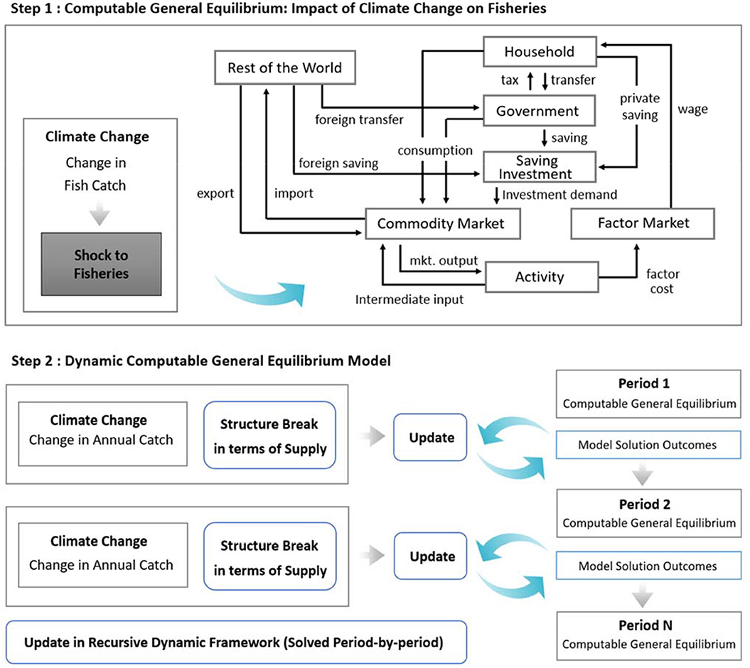
Figure 1. Conceptual framework of CGE for impact of change on fisheries.

Supply

The model covers economic features that reflect the characteristics of the Philippines and the structure follows the approach of Dervis et al. (1982), Robinson (1989), Shoven and Whalley (1992), Ginsburgh and Keyzer (1997), and Lofgren et al. (2002) based on neoclassical perspective. On the side of supply, the model is established under the assumption of profit maximization. Production involves information of input-output based on factors of production and has flexibility for substitution between the labor and capital. The model assumes a Cobb-Douglas production function for the technology in the production process, so the function is homogeneous of degree one and it has constant returns to scale. The formula for production function can be represented as follows:

$\begin{array}{l}{QA}_a={ad}_a·{\displaystyle \prod _f}Q{F}_{fa}^{{\alpha va}_{fa}}\end{array}$

where ad_a is production function efficiency, αva_fa is value-added share for factor f in activity a, QA_a is production activity level, and QF_fa is quantity demanded of factor f by production activity a.

In the model, domestic and export commodity have a constant elasticity of transformation (CET). In other word, the distribution of theses commodities is modeled in the form of CET function, so output transformation can be represented by the function of the quantity of exports and the quantity of domestic output as follows:

$\begin{array}{l}{QX}_c={at}_c·{(\alpha t{r}_c^t\cdot E{X}_c^{{\rho }_c^t}+(1-\alpha t{r}_c^t)\cdot Q{D}_c^{{\rho }_c^t})}^{1/{\rho }_c^t}\end{array}$

where at_c is shift for output transformation, $\alpha t{r}_c^t$ is share for output transformation, ${\rho }_c^t$ is exponent for output transformation, QX_c is the quantity of domestic output, QD_c is the quantity of domestic output sold domestically, and EX_c is the quantity of exports.

Market is represented by perfect competition. Consequently, incidental assumptions are required to develop the model. If price of an input changes then the quantity of the output sold alters, and that affects demand for the input (Hoffmann, 2003). The model assumes the impact of input price is insignificant and firms do not make economic profit, not measuring elasticity of demand which reflects the market power that firms have.

Demand

On the side of demand, the model consists of household, government and the foreign sector reflecting the consumption of domestic good and imported good. Households are classified depending on region. They are divided into two groups: urban and rural household. The government of the model has similar expenditure to the household and gets money through taxation and consumes commodity quantities paying market prices and transfers to households according to the expenditure function. Foreign sector in the model also purchases domestically produced commodity.

The demand side can be represented by the combination of domestic commodity use as follows:

$\begin{array}{l}{QD}_c={\displaystyle \sum _a}{IC}_{ca}+{\displaystyle \sum _h}{QH}_{ch}+{gdo}_c+{QI}_c\end{array}$

where QD_c is domestic sales of domestic output, IC_ca is intermediate use of commodity c by activity a, QH_ch is quantity of consumption of commodity c by household h, gdo_c is government demand for commodity, and QI_c is investment demand.

Armington assumption is used for determination of the combination of domestically produced commodity and imported commodity reflecting responses of trade to price changes. Composite supply takes the form of Armington function as follows:

$\begin{array}{l}{QQ}_c={aq}_c·{(\alpha c{o}_c^q\cdot I{M}_c^{-{\rho }_c^q}+(1-\alpha c{o}_c^q)\cdot Q{D}_c^{-{\rho }_c^q})}^{-1/{\rho }_c^q}\end{array}$

where QQ_c is quantity supplied to domestic commodity demanders, aq_c is shift parameter for composite supply, $\alpha c{o}_c^q$ is share parameter for composite supply, ${\rho }_c^q$ is exponent (−1 < ρ < ∞) for composite supply, and IM_c is quantity of imports, and QD_c is domestic use of domestic output. Due to the equilibrium of demand and supply (i.e., QD_c = QQ_c), the demand side is connected with Armington assumption.

Government

Government also plays a role as an economic agent in general equilibrium. Government consumes commodities while it obtains revenue by collecting tax and transfer. Government revenue and expenditure are represented as follows:

$\begin{array}{l}YG={\displaystyle \sum _h}{tdh}_h·{YH}_h+CR·{tr}_{g,r}+{\displaystyle \sum _c}{tco}_c·({PD}_c·{QD}_c\\ +{({PM}_c·{IM}_c)}_{|c\in CM})\\ +{\displaystyle \sum _c}{tim}_c·CR·{pm}_c·{IM}_c+{\displaystyle \sum _c}{tix}_c·CR·{pe}_c·{EX}_c\end{array}$

where YG is government revenue, tdh_h is the income tax rate of household, tr_{g, r} is transfer from government to rest of world, tco_c is the rate of consumption tax, tim_c is the tariff rate on import, pm_c is import price, tix_c is the rate of tax on exports, pe_c is price of exports, CR is the exchange rate, PD_c is the price of domestic output, QD_c is the quantity of domestic output sold domestically, PM_c is the price of imports in domestic currency, IM_c is the quantity of imports, and EX_c is the quantity of exports.

$\begin{array}{l}GX={\displaystyle \sum _{\text{h}}}{\text{t}\text{r}}_{\text{h},\text{g}}+{\displaystyle \sum _{\text{c}}}{\text{g}d\text{o}}_{\text{c}}•{\text{P}\text{C}}_{\text{c}}\end{array}$

where GX is government expenditure tr_{h, g} is transfer from household to government, gdo_c is government demand for commodity, and PC_c is price of composite commodity c.

Market Clearing

In the CGE model, some constraints are considered for the equilibrium. One of important constraints is the market clearing, so the model assumes market clearing in the factor market and the commodity market. The condition of the factor market clearing can be represented by the equality of supply and demand of factor as follows:

$\begin{array}{l}{FS}_f={\displaystyle \sum _a}{QF}_{fa}\end{array}$

where FS_f is supply of factor f and QF_fa is quantity demanded of factor f by activity a.

The condition of the commodity market clearing comes from relationship between two equations in demand, and it can be represented as follows:

$\begin{array}{l}{QQ}_c={\displaystyle \sum _a}{IC}_{ca}+{\displaystyle \sum _h}{QH}_{ch}+{gdo}_c+{QI}_c\end{array}$

where QQ_c is quantity supplied to domestic commodity demanders, IC_ca is intermediate use of commodity c by activity a, QH_ch is quantity of consumption of commodity c by household h, gdo_c is government demand for commodity, and QI_c is investment demand.

Data

In the study, the one country, multi-sector and recursive CGE model is constructed. For the analysis, information of the value of all transactions in an economy is required. Thus, it is necessary to utilize a social accounting matrix (SAM) which indicates a logical framework of rows and columns providing a visual display of the transactions as a circular flow of national income and spending in an economy (Burfisher, 2017). In this study, the model uses SAM by modification of the 2013 Social Accounting Matrix from the compilation of the Agricultural Model for Policy Evaluation which is constructed by Briones (2016). It provides a set of transactions between fisheries, industry and service sub-sectors in the Philippines. The SAM includes the primary sector, the manufacturing and industry sector, the service sector, and the public sector. The primary sector encompasses the capture fisheries and aquaculture fisheries and other primary sector such as the agriculture. Parameters are drawn from SAM with econometric analysis, and the effect of marine capture fisheries is calculated by interpolation because values of capture fisheries sector are aggregated in the SAM. The modeling⁴ is based on standard hypotheses of CGE and the model is solved in Generalized Algebraic Modeling System (GAMS).

After the construction of the general equilibrium, GDP is calculated by sum of the value of final demands and net exports as follows:

$\begin{array}{l}GDP={\displaystyle \sum _h}{\displaystyle \sum _c}P{C}_{c}Q{H}_{c,h}+{\displaystyle \sum _a}{\displaystyle \sum _c}{\displaystyle \sum _h}C{A}_{ac}QH{A}_{ach}\\ +{\displaystyle \sum _c}P{C}_{c}Q{G}_c+{\displaystyle \sum _c}P{C}_{c}Q{I}_c+{\displaystyle \sum _c}P{C}_{c}qs{t}_c\\ +{\displaystyle \sum _h}{\displaystyle \sum _c}P{C}_{c}Q{H}_{c,h}+{\displaystyle \sum _c}P{M}_{c}I{M}_c+{\displaystyle \sum _c}P{E}_{c}E{X}_c\end{array}$

where PC_c is composite commodity price, QH_ch is quantity of commodity consumption by household, CA_ac is marginal cost of commodity from activity, QHA_ach is quantity of household consumption of commodity from activity for household, QG_c is government consumption demand for commodity, QI_c is quantity of investment demand, PM_c is price of imports in domestic currency, IM_c is quantity of imports, PE_c is price of exports in domestic currency, EX_c is quantity of exports, and qst_c is quantity of stock change.

Results

Philippines Economy

In the simulations, results show more negative change in economic variables where more extreme changes in climate occur. Since three scenarios are applied in this study, the model focuses on the results on differences in GDP. The result of simulation is shown in Figure 2. Ceteris paribus except change in production of fisheries resulted from climate change, baseline scenario is normalized in the analysis. Index score of 100 is set based on GDP of baseline specifying 100 as a reference point. So, the score of 100 means the level of GDP in baseline for each year, and scores <100 indicate the levels in scenarios are underperforming the comparison in the year. As it shows, higher radiative forcing value causes lower level of GDP compared to baseline scenario assuming no changes in the status quo.

FIGURE 2

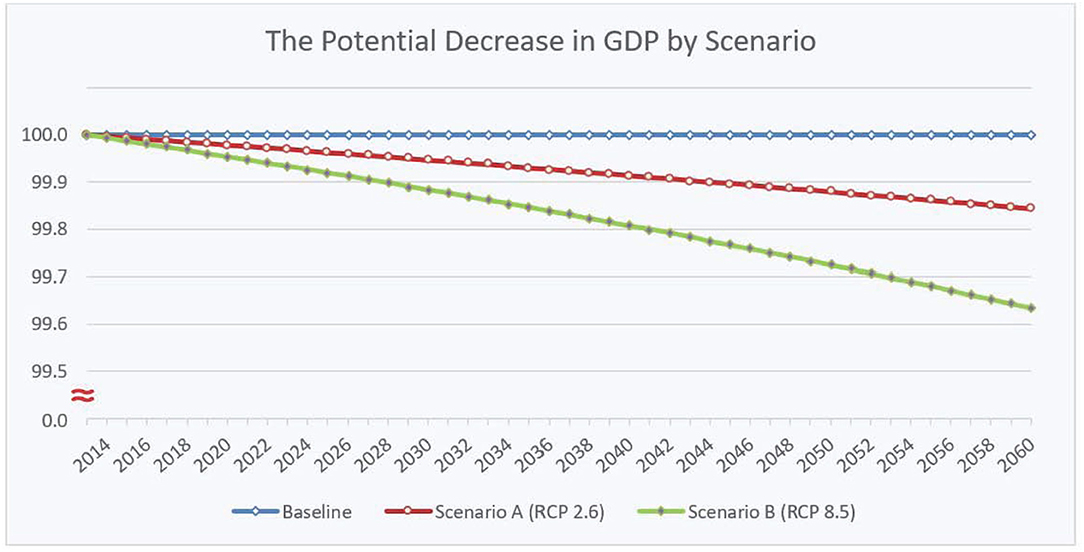
Figure 2. Projection of decrease in GDP by scenario.

As a result of simulation, GDP is expected to decrease by 0.16% with scenario A (RCP 2.6) and 0.37% with scenario B (RCP 8.5) up to 2060. This state came from direct effect, i.e., reduction in catch in exclusive economic zone and seas in the Philippines leading to dwindling supplies, and indirect effect i.e., effects that came about as other product and factor markets in the Philippines respond to the change in productivity.

For the examination of distributional aspects between urban and rural area, households are grouped by residence. Looking at consumption patterns, the nation's service sector seems most active, and that is especially predominant in urban areas. It is shown that rural households spend more on the primary sector and manufacturing and industry sector compared to urban households. On the other hand, urban households appear to spend more on the service sector. To review the fisheries sector, urban households and rural households are on nearly the same share of household consumption spending on fishery commodities. The share of household expenditure allocated to fisheries indicates about 1.4% (Table 1). Urban households spend more on aquaculture products (0.83%) compared to rural households (0.80%), while rural households relatively spend more on marine capture products (0.67%) compared to urban household (0.54%), but there is no significant difference between patterns on the whole.

TABLE 1

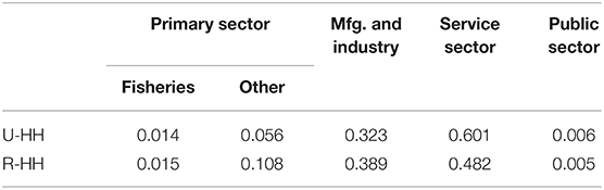
Table 1. Share of household consumption spending on commodity.

Table 2 presents the household income related with the fisheries sector normalized to 100 for the baseline scenario. Ceteris paribus, the result implies that the more global warming, the greater loss of income that will occur. That is to say, climate change has an effect of income reduction. The rate of decrease in income of rural household is 0.163 and 0.372, for scenario A (RCP 2.6) and scenario B (RCP 8.5), respectively; while for the rate of decrease in income of urban household, is 0.160 and 0.360, for scenario A and B, respectively.

TABLE 2

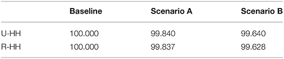
Table 2. Distribution of household income in the fisheries by scenario.

Marine Capture Fisheries Sector

Marine capture fisheries in the simulation represents fisheries excluding inland capture and aquaculture. This follows a classification of the fisheries subsector used in the fisheries situation report issued by the Philippine statistics authority (PSA, 2014). According to the volume of fisheries production data in the Philippines (1980–2010), capture fisheries have made up a high percentage (82%) of the total fisheries production for three decades, and the percentage of marine capture fisheries is 89% and that of inland fisheries is 11% among capture fisheries. The percentage of capture fisheries is decreasing recently, while that of aquaculture is growing. In 2013, capture fisheries accounts for 59% of the total fisheries production in terms of the value of production at constant prices, but based on capture fisheries, marine capture fisheries became more dominant showing 95% of total capture fisheries (PSA, 2014).

Climate change is one of the underlying causes of decrease in production in the marine capture fisheries sector, and the impact of climate change on marine capture fisheries sector is substantial since production is a big part of the economy. In the Philippines, marine capture is currently dominated by roundscad, big-eyed scad, anchovy, Indian oil sardines, Indian mackerel, threadfin bream and tuna species (PSA, 2017a). Production of anchovy is greatly affected by climate change compared to big-eyed scad, Indian mackerel and threadfin bream. Sardine is relatively less vulnerable compared to anchovy but weak upwelling conditions can affect its population. With warmer water and less oxygen available, tuna species in the Philippines (frigate tuna, eastern little tuna, yellowfin tuna, skipjack, bigeye tuna), making 28% of the catch (PSA, 2017a), are expected to decrease due to the shortage of microscopic plants and animals which are an integral part of the tuna food webs (Vousden, 2018).

The marine capture fisheries sector is affected directly by decrease in production while other sectors of the Philippines economy are influenced by only indirect effect. Thus, looking over the marine capture sector, the economic impact of climate change is significant in terms of the ratio. As a result of the simulation, the contribution of marine capture to GDP is expected to decrease by 9.41% with scenario A and 17.95% with scenario B up to 2060 (Figure 3).

FIGURE 3

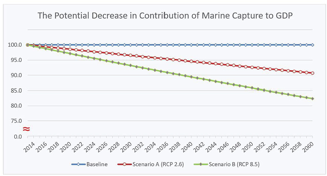
Figure 3. Projection of decrease in contribution of marine capture to GDP by scenario.

The decrease in contribution of marine capture to GDP leads to the decrease in income of fishermen. Fishermen in the Philippines, one of the poorest groups in the nine basic sectors, belong to households with income below the official poverty threshold, representing a poverty incidence of 34% (PSA, 2017b). Thus, a decrease in contribution of marine capture to GDP has a negative impact on the mitigation of poverty incidence, and that means climate change adds to the social welfare in the Philippines.

Climate change brings negative consequences in terms of rural household income (Figure 4). Decreases in productivity leads to income reduction of households engaged in fisheries, dampening profitability of fishing industries. Considering fishermen reside more in rural areas rather than urban areas, it is expected that climate change affects income of rural households more than urban households. Income of rural households is liable to decrease as climate change continues, and it is expected to deepen as climate change becomes extreme.

FIGURE 4

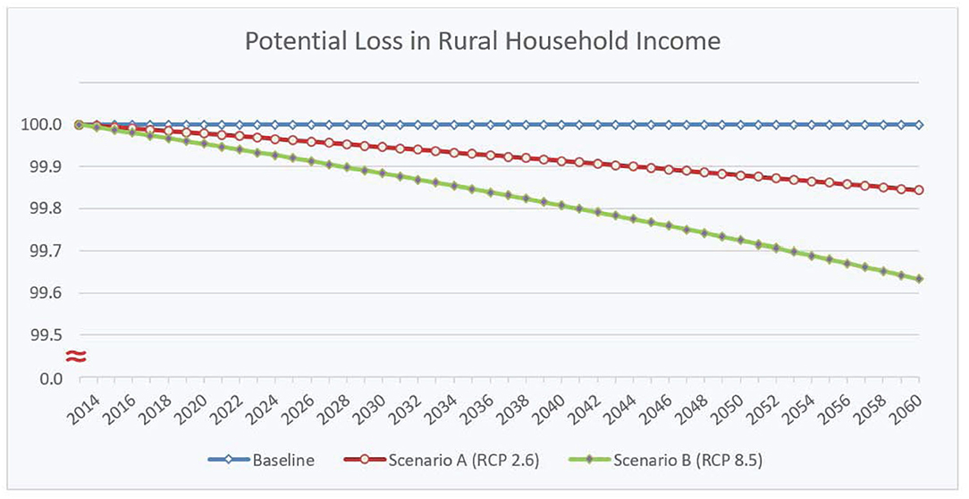
Figure 4. Projection of loss in rural household income by scenario. Income level in base year is normalized to 100.

Capture-Aquaculture Combined Fisheries Sector

In order to examine the impact of climate change on the production of marine capture fisheries, a simulation about capture-aquaculture combined fisheries is carried out. Capture-aquaculture combined fisheries in this section refers to all kinds of fisheries traded in the Philippine market and Filipino fisheries exported to the world market. As shown by the simulation of the economic sector, GDP of the Philippines is expected to decrease from 0.16 to 0.37% compared to the baseline scenario. In light of the proportion of the fisheries sector (which is about 1.8%) to the national economy, there is a huge amount of influence on the economy. Fisheries GDP is expected to decrease by about 9.27% with scenario A and bout 17.65% with scenario B up to 2060 compared to the baseline (Figure 5).

FIGURE 5

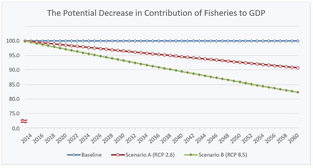
Figure 5. Projection of decrease in contribution of capture-aquaculture combined fisheries to GDP by scenario.

Economic growth is an increase in the production of goods and services due to an improvement in production capacity, and is represented by an increase in GDP. The current Philippines economic data suggests that the fisheries sector will continue to grow due to a rise in demand, an increase in productive capacity, and the development of new technology. Economic growth in fisheries is expected to slow compared to the baseline scenario since climate change brings negative effects. Figure 6 shows economic growth in the fishing sector based on capture indicating inflation-adjusted measures in a corresponding year, i.e., the increase in real GDP. As shown in Figure 6, the model notes that economic growth in the fisheries slopes upward in all scenarios, but the curves in the scenario A and B show relatively slower economic growth.

FIGURE 6

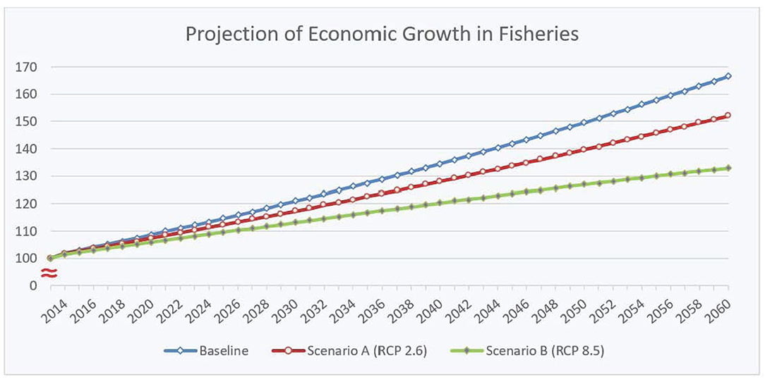
Figure 6. Projection of economic growth in the fisheries by scenario. The GDP in base year is normalized to 100.

Like the marine capture fisheries sector, loss of income affects rural households slightly more than urban households as climate change continues. It implies that climate change can cause urban-rural income disparity. This is because there are more people who work in fisheries in rural areas than urban areas and a decrease in fish catch affects rural household income. Thus, climate change has more negative effect on rural households in terms of fisheries. Figure 7 represents loss in rural household income by scenarios A and B. As shown in the figure, climate change has negative effect of income.

FIGURE 7

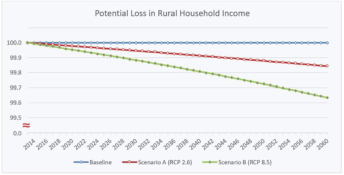
Figure 7. Projection of loss in rural household income by scenario. Income level in base year is normalized to 100.

Discussion

Vicious Circle in Fisheries Sector

The economy of the Philippines has grown for the last decade, but more than 20% of the Philippines population remains poor and the Philippines does not show big dynamism in improvement of economic security, rise in the middle class and even elimination of poverty, compared to other East Asian countries (World Bank, 2016, 2018). The problem is that the poor in the Philippines (30.8% of the population was economically vulnerable, 18.7% was moderately poor, and 6.6% of the population was extremely poor) are more vulnerable to negative shocks being exposed to more risks for shortage of resources without ability to cope and capacities necessary to adapt to potential risks (World Bank, 2018). In other words, climate change leads to problems for the collective economy of the Philippines represented by slow economic growth and deterioration of income distribution. In addition, climate change contributes to accelerating the plight of the poor in the Philippines.

The issue related with climate change and fisheries resulting from this study is the slowdown in economic growth in the fisheries sector. The problem is that for poor households in rural regions, a large share of income comes from activities associated with the primary sector (World Bank, 2018). Therefore, it is expected that factors such as climate change will contribute to the plight of the poor in the Philippine due to slow growth of fisheries and the poor's dependency on fisheries sector. The second problem is the fact that negative economic impacts on the fisheries sector may affect fishery resources in Philippines making a vicious cycle since changes in fish abundance and location will cause more completion and conflict for the remaining resources. It would result in a decline in food resources and food security. Decrease in fish products, which are the means of inexpensive and nutritious food supply, causes significant strain on the cost of living of low-Income people in the Philippine due to limited options in terms of food consumption. Thus, poor fisheries productivity caused by climate change is expected to affect the nation's economy but particularly bring hardships to the poor.

Limitations on the Model

Several points are worth noting to contemplate what are the limitations and how they could be extended in future work. The paper assumed perfect competition in the market of the Philippines. In reality, it may be natural to face different types of market structure that do not meet rigorous criteria of perfect competition. It is necessary to incorporate cases of imperfect markets such as price controls, if applicable. It is also necessary to consider the more flexible and complex functional form of analysis, as well as Cobb-Douglas functions, to better reflect the structure of the Philippine economy.

Second, the paper assumed productivity of all sectors except fisheries, which remains constant, i.e., supply of other fields might be altered under the model mechanism, but it does not mean they are directly affected by climate change. The assumption is advantageous for identifying the influence on fisheries, but leaves something to be desired if someone wants to completely examine the state of the economy itself. To improve predictive power of the model and better represent comprehensive economic condition, it is necessary to consider all products being influenced by climate change, such as agricultural products, simultaneously. Also, the paper assumed paradigm of general equilibrium depending on aggregated data. It is necessary to note that a possibility of spatial variation in fisheries productivity and decline in fisheries is inherent in reality.

Third, the adaption needs to be discussed in depth. This study focuses on assessment of the economic impact by means of the CGE model by reflecting changes in fish catch due to climate change. The model used in this study is reflective of dynamic reaction to change in factors like labor, capital and inputs. However, the adjustment is limited to the changes within the system built to reproduce the economy. Consequently, the adjustments that can progress beyond the current structure is not mechanically reflected in the model as when dealing with non-monetary objectives such as adaptation to climate change. Different adaptabilities could result in change in market structure according to learning effect, change in preference, and new policies. Simulations are performed under the assumption that the current condition persists, but it would be desired to include many situations. It is necessary to reflect various situations with collecting information for any future study.

Conclusion and Recommendation

This paper examined economic impacts of climate change on fisheries in the Philippines applying the dynamic computable general equilibrium (CGE) model. In the analysis, one baseline scenario and two climate change scenarios based on greenhouse gas concentration were considered. The study focused on GDP and income distribution by sector, which can represent economic conditions in terms of economic growth and distribution.

The climate change impacts on marine capture fisheries in the Philippines is projected to cause a decrease by about 9% of fisheries GDP with the mitigation scenario and about 18% of GDP with the extreme scenario up to 2060, compared to the baseline scenario. This impact results in income reduction by as much as 0.36% for urban households and 0.38% for rural households in the Philippine economy. In addition, urban-rural income disparity increases because loss for rural households is slightly higher than that of urban households.

Climate change will affect the fisheries over a long period of time. Accordingly, it means that the Philippines must prepare itself to get ready for the impact and endeavor to mitigate climate change. To prepare for climate change, the Philippine needs to: (i) conduct an assessment of vulnerability to climate change for fisheries at the national level in order to respond to changing economic conditions expected to worsen over time and that the assessment is continuously and periodically carried out; (ii) carry out a gap analysis on the capability to cope with the impact of climate change on fisheries for the national economy; the gap analysis enables organizations to take the selective and premeditated actions providing the information about whether a sector or area can potentially be associated with the issue or which community is more vulnerable to climate change; (iii) make effective management plans for fisheries to develop adaptation to climate change with the accumulated information in the process—for an effective plan, it is necessary to establish reliable research materials by collecting climate data and fisheries-related information, and these sources should be open to both organizations and the public to help make more informed fisheries management decision; (iv) incorporate climate change impacts into national economic development plans and fisheries development plans; and (v) incorporate climate adaptation into the fisheries management plan—it should be accompanied by education on climate change that can increase awareness of impacts of climate change and promotion of adaptation strategies that can reduce the effect of climate change on fisheries.

Data Availability Statement

The datasets generated for this study are available on request to the corresponding author.

Author Contributions

DS and RP have made a substantial contribution to the research work and they were both involved in drafting and editing of the manuscript.

Conflict of Interest

The authors declare that the research was conducted in the absence of any commercial or financial relationships that could be construed as a potential conflict of interest.

Acknowledgments

We sincerely thank Dr. F. Shah (University of Connecticut) for his advice on general equilibrium analysis in the theory.

Footnotes

1. ^According to the prevalence of undernourishment data, in 2017, about 13.5% of the population was malnourished in the Philippines [World Bank (n.d.), “Prevalence of undernourishment”], and fish provides Filipino people with approximately one-third of their average per capita intake of animal protein (Bennett et al., 2018).

2. ^Capture fisheries includes not only marine capture fisheries but also inland capture fisheries. This paper focuses on marine capture fisheries which is dominant in capture fisheries – according to fisheries situation report (PSA, 2014), it shows 95% of capture fisheries.

3. ^El Niño is associated with warming in the tropical Pacific Ocean, and has global climatic teleconnections, affecting the global climate change (Yeh et al., 2009). Sea Surface Temperature (SST) in Southeast Asia has shown an extreme trend due to El Niño (Thirumalai et al., 2017).

4. ^The model includes 27 equations to form the system. Most parameters, variables and equations and the code for the model are developed based on Lofgren et al. (2002) and Lofgren (2003) following the neoclassical structure which is well-developed by Dervis et al. (1982).

References

Adelman, I., and Robinson, S. (1978). Income Distribution Policy in Developing Countries: A Case Study of Korea. Stanford, CA: Stanford University Press.

Google Scholar

Arnason, R. (2006). “Global warming, small pelagic fisheries and risk,” in Climate Change and the Economics of the World's Fisheri‘es: Examples of Small Pelagic Stocks, eds R. Hannesson, M. Barange, and S. Herrick (Northampton, MA: Edward Elgar), 1–32.

Google Scholar

Arnason, R. (2007). Climate change and fisheries: assessing the economic impact in Iceland and Greenland. Nat. Resour. Model. 20, 163–197. doi: 10.1111/j.1939-7445.2007.tb00205.x

CrossRef Full Text | Google Scholar

Badjeck, M. C., Allison, E. H., Halls, A. S., and Dulvy, N. K. (2010). Impacts of climate variability and change on fishery-based livelihoods. Mar. Policy 34, 375–383. doi: 10.1016/j.marpol.2009.08.007

CrossRef Full Text | Google Scholar

Ballard, C. L., Fullerton, D., Shoven, J. B., and Whalley, J. (1985). “Data on household income and expenditure, investment, the government, and foreign trade,” in A General Equilibrium Model for Tax Policy Evaluation (Chicago, IL: University of Chicago Press), 90–112. doi: 10.7208/chicago/9780226036335.001.0001

CrossRef Full Text | Google Scholar

Barange, M., Merino, G., Blanchard, J. L., Scholtens, J., Harle, J., Allison, E. H., et al. (2014). Impacts of climate change on marine ecosystem production in societies dependent on fisheries. Nat. Clim. Change 4, 211–216. doi: 10.1038/nclimate2119

CrossRef Full Text | Google Scholar

Barange, M., and Perry, R. I. (2009). Physical and ecological impacts of climate change relevant to marine and inland capture fisheries and aquaculture. Clim. Change Implic. Fish. Aquacul. 503, 7–106. Retrieved from: http://www.lis.edu.es/uploads/07483fb7_72a2_45ca_b8e7_48bf74072fd3.pdf#page=15

Google Scholar

Bennett, A., Patil, P., Kleisner, K., Rader, D., Virdin, J., and Basurto, X. (2018). Contribution of Fisheries to Food and Nutrition Security: Current Knowledge, Policy, and Research. Nicholas Institute Report 18-02. Durham, NC: Duke University.

Google Scholar

Berrittella, M., Bigano, A., Roson, R., and Tol, R. S. (2006). A general equilibrium analysis of climate change impacts on tourism. Tourism Manage. 27, 913–924. doi: 10.1016/j.tourman.2005.05.002

CrossRef Full Text | Google Scholar

BFAR (2016). Philippine Fisheries Profile 2015. Quezon: Bureau of fisheries and aquatic resources.

Google Scholar

Brander, K. M. (2007). Global fish production and climate change. Proc. Natl. Acad. Sci. U.S.A. 104, 19709–19714. doi: 10.1073/pnas.0702059104

PubMed Abstract | CrossRef Full Text | Google Scholar

Briones, R. M. (2016). Embedding the AMPLE in a CGE Model to Analyze Intersectoral and Economy-Wide Policy Issues. PIDS Discussion Paper Series, No. 2016-38. Makati: Philippine Institute for Development Studies.

Google Scholar

Burfisher, M. E. (2017). Introduction to Computable General Equilibrium Models. New York, NY: Cambridge University Press.

Google Scholar

Cheung, W. W., Lam, V. W., Sarmiento, J. L., Kearney, K., Watson, R. E. G., Zeller, D., et al. (2010). Large-scale redistribution of maximum fisheries catch potential in the global ocean under climate change. Glob. Change Biol. 16, 24–35. doi: 10.1111/j.1365-2486.2009.01995.x

CrossRef Full Text | Google Scholar

Cuvin-Aralar, M. L. A., Ricafort, C. H., and Salvacion, A. (2016). An Overview of Agricultural Pollution in the Philippines: The Fisheries Sector. Washington, DC: World Bank.

Google Scholar

Dellink, R., Hofkes, M., van Ierland, E., and Verbruggen, H. (2004). Dynamic modelling of pollution abatement in a CGE framework. Econ. Model. 21, 965–989. doi: 10.1016/j.econmod.2003.10.009

CrossRef Full Text | Google Scholar

Dervis, K., De Melo, J., and Robinson, S. (1982). General Equilibrium Models for Development Policy. New York, NY: Cambridge University Press.

Google Scholar

Dessus, S., and Bussolo, M. (1998). Is there a trade-off between trade liberalization and pollution abatement?: a computable general equilibrium assessment applied to Costa Rica. J. Policy Model. 20, 11–31. doi: 10.1016/S0161-8938(96)00092-0

CrossRef Full Text | Google Scholar

Dunne, J. P., John, J. G., Adcroft, A. J., Griffies, S. M., Hallberg, R. W., Shevliakova, E., et al. (2012). GFDL's ESM2 global coupled climate–carbon earth system models. Part I: Physical formulation and baseline simulation characteristics. J. Clim. 25, 6646–6665. doi: 10.1175/JCLI-D-11-00560.1

CrossRef Full Text | Google Scholar

Dunne, J. P., John, J. G., Shevliakova, E., Stouffer, R. J., Krasting, J. P., Malyshev, S. L., et al. (2013). GFDL's ESM2 global coupled climate–carbon earth system models. Part II: carbon system formulation and baseline simulation characteristics. J. Clim. 26, 2247–2267. doi: 10.1175/JCLI-D-12-00150.1

CrossRef Full Text | Google Scholar

Dwyer, L., Forsyth, P., and Spurr, R. (2005). Estimating the impacts of special events on an economy. J. Travel Res. 43, 351–359. doi: 10.1177/0047287505274648

CrossRef Full Text | Google Scholar

Eboli, F., Parrado, R., and Roson, R. (2010). Climate-change feedback on economic growth: explorations with a dynamic general equilibrium model. Environ. Dev. Econ. 15, 515–533. doi: 10.1017/S1355770X10000252

CrossRef Full Text | Google Scholar

Eme, J., and Bennett, W. A. (2009). Critical thermal tolerance polygons of tropical marine fishes from Sulawesi, Indonesia. J. Thermal Biol. 34, 220–225. doi: 10.1016/j.jtherbio.2009.02.005

CrossRef Full Text | Google Scholar

FAO (2016). The State of World Fisheries and Aquaculture 2016. Contributing to Food Security and Nutrition for All. Rome: FAO.

Google Scholar

Ganachaud, A. S., Sen Gupta, A., Orr, J. C., Wijffels, S. E., Ridgway, K. R., Hemer, M. A., et al. (2011). “Observed and expected changes to the tropical Pacific Ocean,” in Vulnerability of Tropical Pacific Fisheries and Aquaculture to Climate Change, ed J. D. Bell, J. E. Johnson, A. S. Ganachaud, P. C. Gehrke, A. J., Hobday, O. Hoegh-Guldberg, et al. (Noumea: Secretariat of the Pacific Community), 101–187.

Google Scholar

Geronimo, R. C. (2018). Projected Climate Change Impacts on Philippine Marine Fish Distributions. Quezon: Department of Agriculture – Bureau of Fisheries and Aquatic Resources.

Google Scholar

Ginsburgh, V., and Keyzer, M. (1997). The Structure of Applied General Equilibrium. Cambridge: Massachusetts Institute of Technology.

Google Scholar

Hoegh-Guldberg, O., Poloczanska, E. S., Skirving, W., and Dove, S. (2017). Coral reef ecosystems under climate change and ocean acidification. Front. Mar. Sci. 4:158. doi: 10.3389/fmars.2017.00158

CrossRef Full Text | Google Scholar

Hoffmann, A. N. (2003). Imperfect competition in computable general equilibrium models—a primer. Econ. Model. 20, 119–139. doi: 10.1016/S0264-9993(01)00088-8

CrossRef Full Text | Google Scholar

Hudson, E. A., and Jorgenson, D. W. (1974). US energy policy and economic growth, 1975-2000. Bell J. Econ. 5, 461–514. doi: 10.2307/3003118

CrossRef Full Text | Google Scholar

Ibarra, A. A., Vargas, A. S., and Lopez, B. M. (2013). Economic impacts of climate change on two Mexican coastal fisheries: implications for food security. Economics 7, 1–38. doi: 10.5018/economics-ejournal.ja.2013-36

CrossRef Full Text | Google Scholar

IPCC (2013). Climate Change 2013: The Physical Science Basis. Contribution of Working Group I to the Fifth Assessment Report of the Intergovernmental Panel on Climate Change (New York, NY: Cambridge University Press).

Google Scholar

Irz, X., Stevenson, J. R., Tanoy, A., Villarante, P., and Morissens, P. (2007). The equity and poverty impacts of aquaculture: insights from the Philippines. Dev. Policy Rev. 25, 495–516. doi: 10.1111/j.1467-7679.2007.00382.x

CrossRef Full Text | Google Scholar

Kelleher, K., Willmann, R., and Arnason, R. (2009). The Sunken Billions: The Economic Justification for Fisheries Reform. Washington, DC: World Bank.

Google Scholar

Khalil, I., Atkinson, P. M., and Challenor, P. (2016). Looking back and looking forwards: Historical and future trends in sea surface temperature (SST) in the Indo-Pacific region from 1982 to 2100. Int. J. Appl. Earth Observ. Geoinform. 45, 14–26. doi: 10.1016/j.jag.2015.10.005

CrossRef Full Text | Google Scholar

Kumbaroglu, G. S. (2003). Environmental taxation and economic effects: a computable general equilibrium analysis for Turkey. J. Policy Model. 25, 795–810. doi: 10.1016/S0161-8938(03)00076-0

CrossRef Full Text | Google Scholar

Lam, V. W., Cheung, W. W., Reygondeau, G., and Sumaila, U. R. (2016). Projected change in global fisheries revenues under climate change. Sci. Rep. 6:32607. doi: 10.1038/srep32607

PubMed Abstract | CrossRef Full Text | Google Scholar

Lehodey, P., Alheit, J., Barange, M., Baumgartner, T., Beaugrand, G., Drinkwater, K., et al. (2006). Climate variability, fish, and fisheries. J. Clim. 19, 5009–5030. doi: 10.1175/JCLI3898.1

CrossRef Full Text | Google Scholar

Lofgren, H. (2003). Exercises in CGE Modeling Using GAMS. Washington, DC: Intl Food Policy Res Inst.

Google Scholar

Lofgren, H., Harris, R. L., and Robinson, S. (2002). A Standard Computable General Equilibrium (CGE) Model in GAMS. Washington, DC: Intl Food Policy Res Inst.

Google Scholar

Merino, G., Barange, M., Rodwell, L., and Mullon, C. (2011). Modelling the sequential geographical exploitation and potential collapse of marine fisheries through economic globalization, climate change and management alternatives. Sci. Mar. 75, 779–790. doi: 10.3989/scimar.2011.75n4779

CrossRef Full Text | Google Scholar

Mora, C., and Ospina, A. (2001). Tolerance to high temperatures and potential impact of sea warming on reef fishes of Gorgona Island (tropical eastern Pacific). Mar. Biol. 139, 765–769. doi: 10.1007/s002270100626

CrossRef Full Text | Google Scholar

Munday, P. L., Jones, G. P., Pratchett, M. S., and Williams, A. J. (2008). Climate change and the future for coral reef fishes. Fish Fish. 9, 261–285. doi: 10.1111/j.1467-2979.2008.00281.x

CrossRef Full Text | Google Scholar

Nilsson, G. E., Crawley, N., Lunde, I. G., and Munday, P. L. (2009). Elevated temperature reduces the respiratory scope of coral reef fishes. Glob. Change Biol. 15, 1405–1412. doi: 10.1111/j.1365-2486.2008.01767.x

CrossRef Full Text | Google Scholar

Palomares, M. L. D., and Pauly, D. (2014). Philippine Marine Fisheries Catches: A Bottom-Up Reconstruction, 1950 to 2010. Vancouver, BC: University of British Columbia.

Google Scholar

Pankhurst, N. W., and Munday, P. L. (2011). Effects of climate change on fish reproduction and early life history stages. Mar. Freshw. Res. 62, 1015–1026. doi: 10.1071/MF10269

CrossRef Full Text | Google Scholar

Paun, A., Acton, L., and Chan, W. S. (2018). Fragile Planet: Scoring Climate Risks Around the World. London: HSBC Bank Plc.

Google Scholar

Peñaflor, E. L., Skirving, W. J., Strong, A. E., Heron, S. F., and David, L. T. (2009). Sea-surface temperature and thermal stress in the Coral Triangle over the past two decades. Coral Reefs 28:841. doi: 10.1007/s00338-009-0522-8

CrossRef Full Text | Google Scholar

Perry, A. L., Low, P. J., Ellis, J. R., and Reynolds, J. D. (2005). Climate change and distribution shifts in marine fishes. Science 308, 1912–1915. doi: 10.1126/science.1111322

PubMed Abstract | CrossRef Full Text | Google Scholar

Pörtner, H. O., Karl, D. M., Boyd, P. W., Cheung, W., Lluch-Cota, S. E., Nojiri, Y., et al. (2014). “Ocean systems,” in Climate Change 2014: Impacts, Adaptation, and Vulnerability. Part A: Global and Sectoral Aspects, eds C. B. Field, V. R. Barros, D. J. Dokken, K. J. Mach, M. D. Mastrandrea, T. E. Bilir, M. Chatterjee, K. L. Ebi, Y. O. Estrada, R. C. Genova, B. Girma, E. S. Kissel, A. N. Levy, S. MacCracken, P. R. Mastrandrea, and L. L. White (New York, NY: Cambridge University Press), 411–484.

Google Scholar

Pratchett, M. S., Hoey, A. S., and Wilson, S. K. (2014). Reef degradation and the loss of critical ecosystem goods and services provided by coral reef fishes. Curr. Opin. Environ. Sustain. 7, 37–43. doi: 10.1016/j.cosust.2013.11.022

CrossRef Full Text | Google Scholar

Prein, M., and Ahmed, M. (2000). Integration of aquaculture into smallholder farming systems for improved food security and household nutrition. Food Nutr. Bull. 21, 466–471. doi: 10.1177/156482650002100424

CrossRef Full Text | Google Scholar

PSA (2014). Fisheries Situationer, January - December 2014. Quezon: PSA.

Google Scholar

PSA (2017a). Fisheries Situation Report, 2017 January-December. Quezon: PSA.

Google Scholar

PSA (2017b). 2017 Annual Report. Quezon: PSA.

Google Scholar

Robinson, S. (1989). Multisectoral models. Handb. Dev. Econ. 2, 885–947. doi: 10.1016/S1573-4471(89)02005-X

CrossRef Full Text | Google Scholar

Robinson, S., Willenbockel, D., and Strzepek, K. (2012). A dynamic general equilibrium analysis of adaptation to climate change in Ethiopia. Rev. Dev. Econ. 16, 489–502. doi: 10.1111/j.1467-9361.2012.00676.x

CrossRef Full Text | Google Scholar

Roessig, J. M., Woodley, C. M., Cech, J. J., and Hansen, L. J. (2004). Effects of global climate change on marine and estuarine fishes and fisheries. Rev. Fish Biol. Fish. 14, 251–275. doi: 10.1007/s11160-004-6749-0

CrossRef Full Text | Google Scholar

Ruddiman, W. F. (2001). Earth's Climate: Past and Future. New York, NY: W. H. Freeman.

Google Scholar

Santos, M. D., Dickson, J. O., and Velasco, P. L. (2011). “Mitigating the impacts of climate change: Philippine fisheries in focus,” in Fish for the People, ed. C. Pongsri (Bangkok: Southeast Asian Fisheries Development Center), 101–110.

Google Scholar

Sarmiento, J. L., Slater, R., Barber, R., Bopp, L., Doney, S. C., Hirst, A. C., et al. (2004). Response of ocean ecosystems to climate warming. Glob. Biogeochem. Cycles 18. doi: 10.1029/2003GB002134

CrossRef Full Text | Google Scholar

Shoven, J. B., and Whalley, J. (1992). Applying General Equilibrium. New York, NY: Cambridge University Press.

Google Scholar

Siriwardana, M., Meng, S., and McNeill, J. (2011). The Impact of a Carbon Tax on the Australian Economy: Results From a CGE Model. Business, Economics and Public Policy Working Papers. Armidale, NSW: University of New England.

Google Scholar

Stock, C. A., Alexander, M. A., Bond, N. A., Brander, K. M., Cheung, W. W., Curchitser, E. N., et al. (2011). On the use of IPCC-class models to assess the impact of climate on living marine resources. Prog. Oceanog. 88, 1–27. doi: 10.1016/j.pocean.2010.09.001

CrossRef Full Text | Google Scholar

Thirumalai, K., DiNezio, P. N., Okumura, Y., and Deser, C. (2017). Extreme temperatures in Southeast Asia caused by El Niño and worsened by global warming. Nat. Commun. 8, 1–8. doi: 10.1038/ncomms15531

PubMed Abstract | CrossRef Full Text | Google Scholar

Vannuccini, S., Kavallari, A., Bellù, L. G., Müller, M., and Wisser, D. (2018). “Understanding the impacts of climate change for fisheries and aquaculture: global and regional supply and demand trends and prospects,” in Impacts of Climate Change on Fisheries and Aquaculture, ed M. Barange (Rome: FAO), 41–62.

Google Scholar

Vousden, D. (2018). Western and Central Pacific Ocean. Transboundary Diagnostic Analysis. Honiara: Pacific Islands Oceanic Fisheries Management.

Google Scholar

Wendner, R. (2001). An applied dynamic general equilibrium model of environmental tax reforms and pension policy. J. Policy Model. 23, 25–50. doi: 10.1016/S0161-8938(00)00025-9

CrossRef Full Text | Google Scholar

World Bank (2016). Philippines Economic Update: Outperforming the Region and Managing the Transition. Washington, DC: World Bank.

Google Scholar

World Bank (2018). Making Growth Work for the Poor: A Poverty Assessment for the Philippines. Washington, DC: World Bank. doi: 10.1596/29960

CrossRef Full Text | Google Scholar

World Bank (n.d.). “Prevalence of undernourishment,” in World Development Indicators, The World Bank Group. Retrieved from: https://data.worldbank.org/indicator/SN.ITK.DEFC.ZS.

Google Scholar

Yeh, S. W., Kug, J. S., Dewitte, B., Kwon, M. H., Kirtman, B. P., and Jin, F. F. (2009). El Niño in a changing climate. Nature 461, 511–514. doi: 10.1038/nature08316

PubMed Abstract | CrossRef Full Text | Google Scholar