Impact of Freshwater Inflow From the Volturno River on Coastal Circulation

1. Introduction

The hydrodynamics of a river frontal zone is a complex issue due to the interaction between the freshwater of the river outflow and the coastal waters (MacDonald et al., 2013; Horner-Devine et al., 2015). It influences the sediment balance, the distribution of chemical and physical parameters, and the nutrient input, making the area a very productive habitat (McLusky and Elliott, 2004). Furthermore, river plumes constitute a provision of buoyant freshwater which interacts with coastal currents, representing an important dynamic process that influences the nearshore circulation (Gan et al., 2009). Several studies have been carried out on sediment, nutrient, and pollutant dispersal in the river estuary mouth (Wright, 1977; De Pippo et al., 2003; Bainbridge et al., 2012; Devlin et al., 2012), on circulation near the river outflow (Garvine, 2001; Hetland, 2005, 2010; MacDonald and Geyer, 2005; Kelsey-Wilkinson, 2014), and on onshore/offshore shifting of the plume due to winds and tides (Garvine, 1999; Fong and Geyer, 2001; Hetland, 2005; Hetland and Signell, 2005; McCabe et al., 2009; Cole and Hetland, 2016). The impact of the river on biogeochemical parameters (Mangoni et al., 2016; Bonomo et al., 2018; Ferraro et al., 2018) and the hierarchical use of different measurement platforms (Ferrara et al., 2017) have also been analyzed to support water quality monitoring.

The Volturno river is the sixth-longest river in Italy and the longest in the South, with a length of 175 km and an estimated mean discharge of 40 m³s⁻¹ (Iermano et al., 2012). It provides the greatest contribution of freshwater to the area. The nearby Regi Lagni and Agnena channels, the shorter river Garigliano in the north, and the Lago Patria in the south of Volturno (Figure 1) also affect the area with their freshwater inputs. A wide shelf at less than 50 m depth slowly deepens toward the Tyrrhenian basin through a break at 120 m (De Pippo et al., 2003). In the northern part of the Gulf of Gaeta, the seabed morphology shows a double order of bars: the first deeper than 5 m and parallel to the coastline and the second shallower and transverse to the shoreline (Cocco and Pippo, 1988).

FIGURE 1

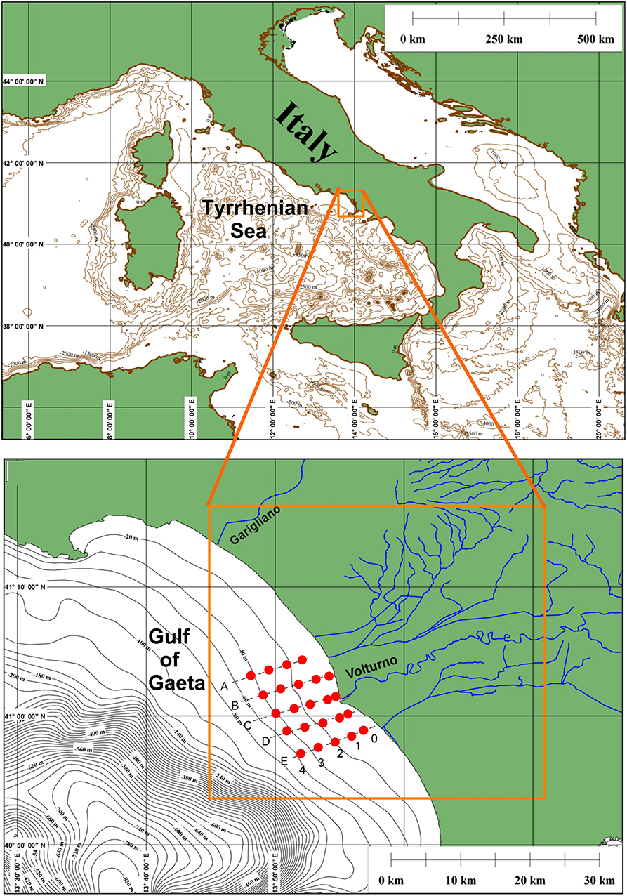
Figure 1. The model domain in the Tyrrhenian Sea (orange square) with bathymetry and CTD casts (red dots).

The catchment basin of the river (~5,550 km²) is densely populated and is highly affected by agropastoral activities, which cause microbiological and chemical contamination (Mancini et al., 1994; Parrella et al., 2003). Knowledge of the connection between stressors from the land and coastal dynamics is an important goal of Integrated Coastal Zone Management (ICZM) and the maintenance of Good Environmental Status (GES), as required by the current Marine Strategy Framework Directive (2008/56/CE, MSFD).

De Pippo et al. (2003) and Iermano et al. (2012) describe the Gulf of Gaeta as constituted by an offshore and a coastal zone. The former, extending from the shelf break, is mainly influenced by a northward flow in winter and a southward flow in summer, linked to the general Tyrrhenian circulation (Hopkins, 1988; Astraldi and Gasparini, 1994). De Pippo et al. (2003) also highlight that the coastal circulation (<50 m) is influenced by cyclonic and anticyclonic eddies, coastal morphology, and submerged morphostructures. Moretti et al. (1977) describe the circulation as also affected by local winds, which form surface currents up to one order of magnitude larger than the mean circulation of the basin.

In this work, we study the spatial and temporal variability of the waters and the impact of the freshwater inflow on the marine vertical stratification by means of in-situ hydrological data from seven synoptical high-resolution surveys (See Table 1). Furthermore, we provide a first assessment of the steady circulation using the Princeton Ocean Model (POM) in a purely diagnostic mode (Ezer and Mellor, 1994; Zavatarelli et al., 2002).

The hydrological (Conductivity Temperature Depth–CTD) dataset and the diagnostic numerical model are described in section 2. Then, the results of the observations and numerical experiments are discussed and reported in section 3. Concluding remarks are provided in section 4.

TABLE 1

Table 1. CTD survey name (first column), temporal periods of acquisition (second column), and wind direction and intensity (third column).

2. Materials and Methods

2.1. The Hydrographic Dataset

Seven synoptic surveys, named I-AMICA, were carried out between June 2012 and October 2014 (Ribotti et al., 2019) (data freely available at https://www.seanoe.org/data/00591/70324/). At least three surveys per year were organized in early summer (June), autumn (October), and winter (February and December), except for autumn 2013 and summer 2014 (Table 1). During each survey, 24 CTD profiles of temperature and absolute salinity (hereafter salinity) were acquired from the surface to the bottom along five transects perpendicular to the coast between 40.85° and 41.10°N in latitude and 13.76 and 14°E in longitude (Figure 1). A quasi-regular grid, ~2 km in longitude and ~3 km in latitude, represents the classic strategy for synoptic ocean sampling. A Seabird SBE11 plus multi-parametric probe was used to acquire physical-chemical parameters on board the R/V Astrea of the Istituto Superiore per la Protezione e la Ricerca Ambientale (ISPRA). Each survey was performed in 1 day and under good weather and sea conditions. A quality check on CTD data has been performed in order to remove possible spikes along the profiles using SBE Data Processing software.

2.2. The Numerical Model

The hydrodynamic model is based on the POM, a non-linear, fully three-dimensional, primitive equation (conservation of mass, momentum, and energy), finite difference model that solves the heat, mass, and momentum conservation equations of fluid dynamics (Blumberg and Mellor, 2013). POM is designed to realistically represent ocean physics, through free surface, baroclinic, terrain-following (sigma) coordinates. The core equations describe the three-dimensional velocity, temperature, salinity, and surface elevation fields, assuming hydrostatic and Boussinesq approximation (Mellor and T. Ezer, 1994; Blumberg and Mellor, 2013). Sub-scale processes are parameterized by eddy coefficients for both momentum and scalar diffusion through the Mellor-Yamada level 2.5 closure scheme (Mellor and Yamada, 1982) for the surface and the bottom mixed layer, which should yield a realistic Ekman surface and bottom layers on the continental shelf. The governing equations are numerically solved using the finite difference method on an Arakawa C-type staggered grid. POM has been successfully and extensively used for coastal and estuarine circulation studies, representing well a wide range of issues such as circulation and mixing processes in rivers, estuaries, shelves and slopes, lakes, semi-enclosed seas, and open and global ocean (Wong et al., 2004; Hordoir et al., 2006; Nekouee et al., 2015; Osadchiev and Korshenko, 2017). Its simple implementation, the use of an embedded turbulence closure model resulting in better Ekman and surface layers, and its computational efficiency are the reasons behind this modeling choice.

POM was implemented within 40.84 to 41.23°N and 13.70 to 14.08°E, with a grid resolution of 1/180° (~600 m). The model domain is represented by the box in Figure 1. Its spatial resolution is set based on analysis of the variability of the Rossby radius of deformation (described in section 3.1) so that it would be possible to resolve the horizontal scale of local coastal processes.

The model is based on a split time step: the external barotropic mode (two-dimensional) uses a short time step for the time evolution of the free surface elevation and the depth-averaged velocity, while the internal mode (three-dimensional) uses a long time step to solve the vertical velocity shear through the equation of continuity, as described in Blumberg and Mellor (2013). Here, the external time step is set to 2.5 s to satisfy the Courant–Friedrichs–Lewy condition associated with the surface wave gravities, while the internal one is set to 25 s. The water column is discretized into 21 sigma levels with a linear distribution from the surface to the bottom.

The bathymetry of the model is based on the U.S. Navy bathymetric database DBDB1 (1' resolution, ~2 km). It is interpolated to the configured grid, and its shallowest depth is set to 5 m to prevent crowding of sigma levels at the minimum depth resolved by the model. In order to define the initial state of temperature and salinity fields in the model, we interpolate the CTD data through the Objective Analysis (OA) method. OA is a numerical procedure of optimal interpolation extensively used by meteorologists (Thiebaux and Pedder, 1988) and oceanographers (Bretherton et al., 1976; Carter and Robinson, 1979) as an interpolator and a smoother of sparse observed temperature and salinity data. The following correlation function (Robinson and Golnaraghi, 1993) is used for each dataset, as the interpolation is applied in space and not in time:

$\begin{array}{ll}f(r)=(1-\frac{r^2}{a^2})exp(-\frac{1}{2}\frac{r^2}{b^2}),& (1)\end{array}$

$\begin{array}{l}{r}^2={(x_1-x_2)}^2+{(y_1-y_2)}^2\end{array}$

where a is the zero-crossing correlation scale or the de-correlation distance (km), b is the decay length scale (km), and r is the distance between two coordinate points, i.e., (x₁, y₁) and (x₂, y₂). In order to generate a correlation matrix defined as positive, a and b must satisfy the condition $a>\sqrt{2}b$ (Bretherton et al., 1976). The values of the parameters a and b in the correlation function of equation (1) are chosen after an accurate sensitivity analysis (not shown). The smaller the area of influence of the observations is, the faster the error increases. The sensitivity test allows us to define a = 15 km and b = 10 km, consistent with the first baroclinic Rossby radius of deformation, as discussed in section 3.1. Furthermore, we select 4 influential points chosen as optimal values for OA fields and all the horizontal OA maps shown in this paper. The interpolated temperature and salinity are mapped on 32 horizontal levels, spaced every ~2 m in the first 30 m depth and every 4 m down to the bottom (~50 m), by means of the OA. In each horizontal level, the fields with a mean error less than 20% are considered. Successively, each field is vertically interpolated from the zeta to sigma levels of the ocean model. This procedure is repeated for each survey to initialize the numerical ocean model.

During the numerical integration, the three-dimensional velocity field associated with each survey is obtained through the full momentum equations of POM in a purely diagnostic mode (Ezer and Mellor, 1994; Zavatarelli et al., 2002). Then the time-dependent processes remain unchanged from the initial state of optimally interpolated temperature and salinity fields until the total velocity (barotropic + baroclinic) field is dynamically adjusted. The kinetic energy is thus dynamically consistent with the initial condition and the wind stress field applied. This methodology is a common practice for the initialization of regional/coastal models with climatological (Mellor, 1991; Ezer and Mellor, 1992) or quasi-synoptic data for nowcast (Onken and Sellschopp, 2001; Sorgente et al., 2016) and forecast experiments (Ezer et al., 1992, 1993; Onken et al., 2005). Running the ocean model in diagnostic mode, rather than the classical geostrophic approach, usually gives more realistic results.

At the surface, POM is forced with a no time-dependent wind stress through the following momentum flux:

$\begin{array}{l}{K}_M\frac{\partial \overrightarrow{u}}{\partial z}{|}_{z=\eta }=\frac{\overrightarrow{\tau }}{{\rho }_0}\end{array}$

where K_M is the vertical kinematic viscosity, ρ₀ is the reference density for the sea water, η is the surface elevation, and $\overrightarrow{\tau }$ is the wind stress. The latter is computed by means of the quadratic bulk formula presented by Hellerman and Rosenstein (1983), using a drag coefficient $C_d=C_d(\overrightarrow{u},T_{air},T_{sst})$ that is a function of the wind velocity amplitude (u) and the air (T_air) and sea surface (T_sst) temperatures. The wind and air temperature fields come from the ERA-Interim analyses of ECMWF, which have a spatial resolution of 0.0125°, while the sea surface temperature (T_sst) field is derived from the above-described CTD data, optimally interpolated into the model grid. Zero surface heat and salinity fluxes are specified at the ocean surface, as they are negligible for the diagnostic calculations (Ezer and Mellor, 1994). Moreover, the wind stress field is computed onto the model grid by bilinear interpolation and averaged over the period of each correspondent survey. During the numerical integration, the wind stress does not change in time at each grid point.

The model has two open boundaries, the western and the southern (Figure 1). Temperature and salinity conditions are defined by the interpolated observations, while the total velocity is defined by the following radiation condition:

$\begin{array}{l}\frac{\partial \overrightarrow{u}}{\partial t}+c_e\frac{\partial \overrightarrow{u}}{\partial x}=0\end{array}$

where $c_e=\sqrt{gH}$, g is the gravitational acceleration (9.8 ms⁻²), and H is the depth. The barotropic velocity is neglected as the wind was weak during our surveys (Table 1). At the seabed, the boundary conditions depend on the bottom friction stress with a spatially variable drag coefficient. This is calculated by assuming a logarithmic bottom boundary layer, using a non-constant bottom roughness, as proposed by Nekouee et al. (2015).

3. Discussion and Results

3.1. Vertical Structure of Temperature and Salinity

In this section, we describe the characteristics of the waters involved in the area and analyze their variability in terms of TS diagram, mean vertical profile, standard deviation (σ), and squared Brunt-Väisälä frequency (BVF). The latter is defined as:

$\begin{array}{l}N=\sqrt{-\frac{g}{{\rho }_0}\frac{\partial \rho }{\partial z}}\end{array}$

where g is the gravitational acceleration (9.8 ms⁻²), ρ₀ is the mean density, and ∂ρ/∂z is the local vertical density gradient from the observed temperature and salinity fields. The BVF is representative of the stability of the water column (Osborn, 1980). All of the mean vertical profiles are estimated by taking the arithmetic average of the observed profiles from 3 m depth down to the bottom.

The TS diagram (Figure 2) identifies different types of waters, which are characterized by strong seasonal variability in terms of density and vertical stability. It shows the typical transitional waters resulting from turbulent mixing between the river freshwater (salinity <34 g kg⁻¹) and the saltier water of the coastal area (salinity > 37.8 g kg⁻¹). As we are analyzing different seasons, we define the transitional waters using salinity instead of the density, as suggested by Budillon et al. (1999).

FIGURE 2

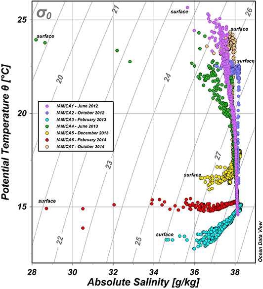
Figure 2. TS diagram for all seven surveys from the surface to the bottom, differently colored.

Two distinct hydrological seasonal conditions are detected: the summer/autumn and the winter. The former is characterized by high vertical thermal stratification, with a decrease of temperature from the surface to the bottom. Temperature is the main driver of the density distribution along the whole water column. Inversely, winter conditions present colder and fresher waters in the upper layer than at the bottom. The buoyant river freshwater strongly modulates the salinity in the surface layer. This is a typical trend for coastal areas subject to river outflows (Fratianni et al., 2016).

During the surveys in June 2012 and 2013 (Table 1), the mean vertical profiles of temperature, salinity, and squared BVF show high vertical stratification (Figure 3). The surface temperature in June 2012 (~24.1°C) is higher (~2°C) than in June 2013 (Figure 3A). Below, the temperature decreases along the water column forming a wide thermocline layer down to the bottom. Here, the temperature is similar during both years (~15°C) and approximates that observed in February 2013 and 2014 (Figure 5A). The salinity (Figure 3B) shows the impact of the freshwater river plume during the two surveys. The most evident effect is observed in June 2013, with the formation of strong vertical stratification. This is characterized by a minimum mean value at the surface (~36.6 g kg⁻¹) and strong spatial variability (σ = 1.8 g kg⁻¹), mainly affecting the halocline down to ~15 m. In this layer, the salinity increases faster than in June 2012. Below this depth, the salinity is approximately constant (~38 g kg⁻¹), with very low variability, for both years. The high stability of the waters is well-represented by the mean vertical profile of the squared BVF (Figure 3C). It ranges between 2 and 4·10⁻³ s⁻², which are the typical values of the North Adriatic Sea (Fratianni et al., 2016). These high values indicate low vertical mixing processes within the pycnocline layer down to ~20 m.

FIGURE 3

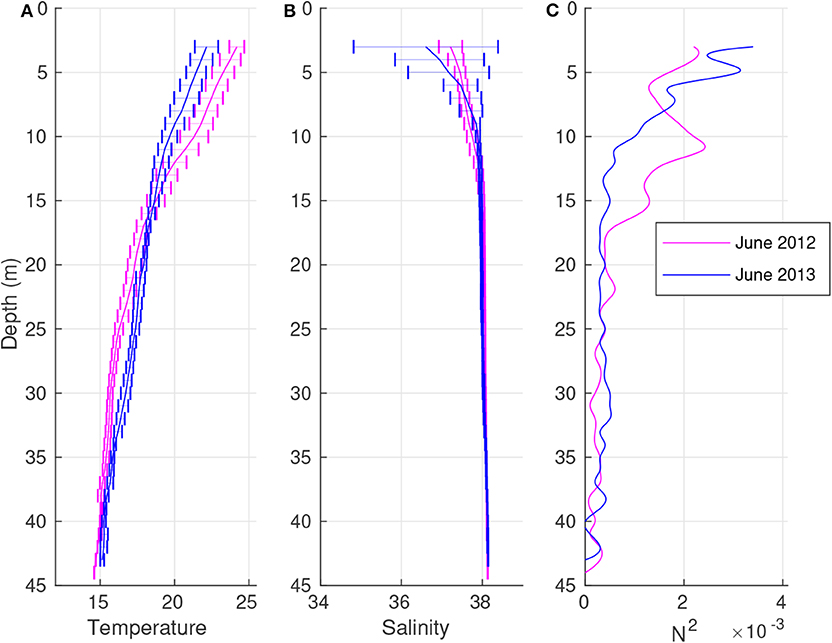
Figure 3. Mean vertical profiles and standard deviations (bars) of temperature (A; °C), salinity (B; g kg⁻¹), and the squared Brunt-Väisälä frequency [C; (s⁻²)] in June 2012 (purple line) and June 2013 (blue line).

An upper isothermal layer down to ~25 m is observed in autumn (Figure 4A) due to heat loss at the sea surface and the turbulent mixing processes. The difference between the mean temperature profiles in the isothermal layer is ~1.4°C, with higher values in October 2014 than in 2012. Below the isothermal layer, the temperature profiles for both of the 2 years decrease down to the bottom, with a remarkable increase in the standard deviation (σ = 1.8°C at 36 m) in October 2014. At the bottom, the temperature is higher than in early summer (~4°C) because of the progressive transfer of heat from the surface during the previous months. The mean profile of salinity is weakly stratified in the upper layer (Figure 4B). The minimum surface salinity is the lowest in October 2014 (S~37.6 g kg⁻¹). The spatial variability is weak (σ <0.22 g kg⁻¹), with higher values toward the surface. The salinity is approximately constant (S~38 g kg⁻¹) along the water column, with a progressive reduction in the standard deviation. The presence of the superficial isothermal layer and the weak vertical stratification of salinity imply low values of squared BVF (Figure 4C) due to the high vertical mixing from the surface down to the upper layer of the pycnocline (~25 m depth).

FIGURE 4

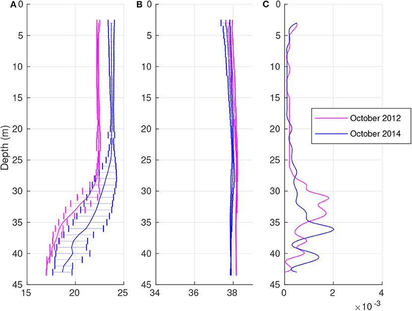
Figure 4. Mean vertical profiles and standard deviations (bars) of temperature (A; °C), salinity (B; g kg⁻¹), and the squared Brunt-Väisälä frequency [C; (s⁻²)] in October 2012 (purple line) and October 2014 (blue line).

For the last three winter surveys, the analysis of mean vertical profiles shows a wide inverse thermocline, which affects most of the water column (Figure 5A). The minimum temperature is observed at the surface, and the lowest (T~13.5°C) is in February 2013, ~1.5°C lower than in February 2014, whereas it is ~16.5°C in December 2013. It increases along the water column, forming a thermal inversion, with cooler waters floating above those that are warmer in the upper layer. In February 2013, the difference in temperature between the surface and the bottom is about +2°C. The water column is also stratified in terms of salinity, with its minimum at the surface (Figure 5B). Its lowest value (S~36.0 g kg⁻¹) is observed in February 2014, with a high spatial variability (σ = 1.5 g kg⁻¹) that decreases down to the bottom. The vertical distribution of salinity preserves the stability of the water column, highlighted by high values of squared BVF, especially in February 2014 (Figure 5C), and comparable with those in June 2013 (see Figure 3C). This isothermal condition is mainly due to the higher freshwater inflow (Figure 6), while salinity increases along the water column, and the BVF is nearly zero below ~15 m.

FIGURE 5

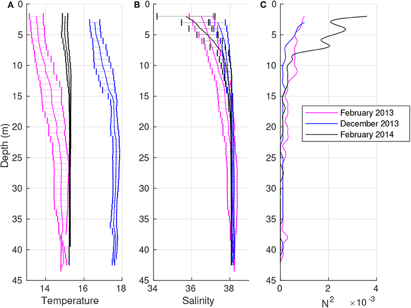
Figure 5. Mean vertical profiles and standard deviations (bars) of temperature (A; °C), salinity (B; g kg⁻¹), and the squared Brunt-Väisälä frequency [C; (s⁻²)] in February 2013 (purple line), December 2013 (blue line), and February 2014 (black line).

FIGURE 6

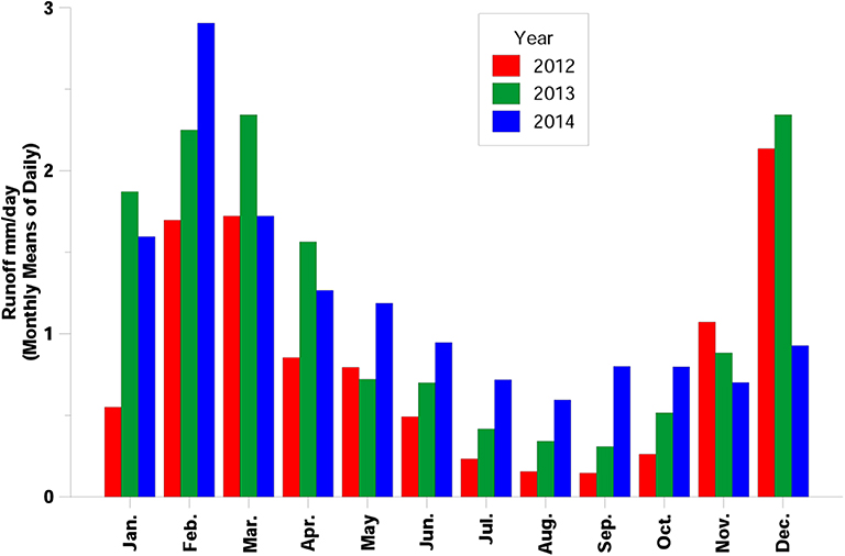
Figure 6. Monthly mean climatology of the surface river runoff for the period 2012–2014. Precipitation is the variable that imposes mm/day to the ERA Interim surface runoff data.

The Rossby radius of deformation is computed by the CTD profiles and provides the fundamental horizontal scale of the dynamic processes in the study area (Gill, 1982; Chelton et al., 1998; Nurser and Bacon, 2014). Its highest values are found in early summer (June 2012, R₁~16.2 km; June 2013, R₁~15.7 km), when the vertical stratification is remarkable. On the contrary, lower values are found in December 2013 (R₁ ~5.5 km), when a well-mixed upper layer is present. Intermediate values are found in winter (February 2013, R₁~9.4 km; February 2014, R₁~7.7 km) and in autumn (October 2012, R₁~11.1 km; October 2014, R₁~11.2 km).

3.2. Analysis of the Impact of the River Plume

The temporal and spatial variability of optimally interpolated temperature and salinity fields at 3 m are described to study the impact of the river freshwater plume on the properties of the waters.

In early summer, the CTD data analysis shows isotherms approximately parallel to the coast, forming a wide thermal front (not shown). In June 2012, it separates the offshore warmer waters from the coastal colder ones, while the opposite occurs in June 2013. Such an inversion is due to the observed decrease in the sea surface temperature in June 2013, which is more intense for the offshore waters. The salinity field is affected by low spatial variability in June 2012, with a signal of transitional waters (S~ 36.9 g kg⁻¹) along the coast (Figure 7A). Freshwater (S~ 33.5 g kg⁻¹) is clearly observed downstream in June 2013 (Figure 7B). Here, downstream means the direction that a Kelvin wave propagates (Fong and Geyer, 2002). Strong horizontal salinity gradients are thus detected between the freshwater core and the surrounding saltier water, although the surface river runoff is weak (Figure 6). The reason for this anomaly is probably the precipitation event that occurred a few days before the survey (not shown). The vertical distributions of the isohalines and the isotherms show the impact of the river freshwater plume on the spatial variability of the waters (Figure 7). In June 2012, isotherms and isohalines move upward toward the coast down to ~20 m, while below that, they are nearly horizontal (Figure 7C). There is weak signal of transitional waters close to the river mouth in the upper 3 m. Vice versa in June 2013, the impact of the plume is more evident (Figure 7D). The transitional waters shape a wide surface layer close to the coast, forming a surface-trapped plume (Chapman and Lentz, 1994). This feature modifies the slopes of the isotherms, progressively inverting them along the water column and inhibiting any vertical mixing between the transitional waters in the upper layer and the deeper and saltier waters of Tyrrhenian origin.

FIGURE 7

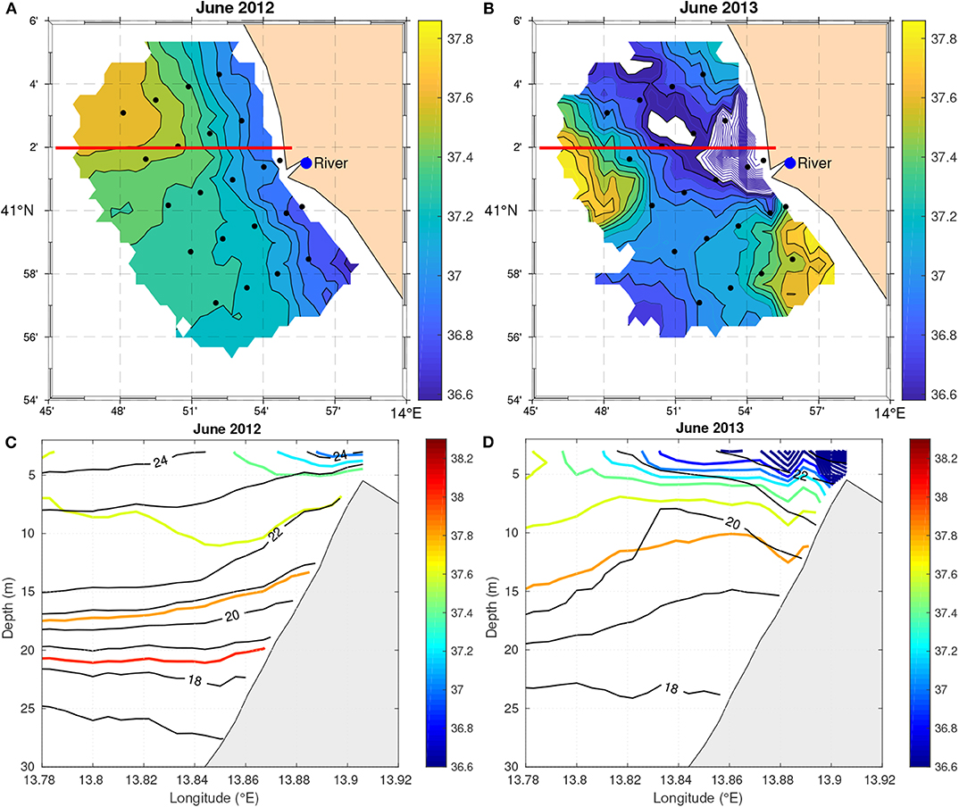
Figure 7. OA maps of salinity (g kg⁻¹) at 3 m (A,B) in June 2012 (left panel) and June 2013 (right panel). The fields are not plotted where the OA expected error exceeds 20%. The contour interval is 0.1 g kg⁻¹. In (B), the salinity below 37 g kg⁻¹ is in correspondence with the three casts in front of the river mouth. It is not drawn to highlight the other structures. Dots indicate location of casts. In (C,D), the vertical isolines of temperature (in black, contour interval 0.05°C) and salinity (colored, contour interval 0.05 g kg⁻¹) are shown for both along the 41° 02' N parallel (red line).

In October 2012, the salinity field shows a river plume characterized by warmer transitional waters (S~37.5 g kg⁻¹, T~22.5°C) that is located in front of the river mouth and a progressive increase in salinity offshore (Figure 8A). In October 2014, there is an evident signal of colder transitional waters (S~37.3 g kg⁻¹, T~23.3°C), slightly upstream of the river mouth (Figure 8B), separated from the surrounding saltier and warmer waters. The vertical sections highlight a shallow (upper 5 m) thermal stratification in October 2012, followed by a wide isothermal layer to ~15 m (Figure 8C). Below, a thin layer of relatively warmer and saltier waters (S~38.1 g kg⁻¹), located offshore, induces a thermal stratification down to the bottom, while salinity is approximately constant (Figure 4). The temperature field is characterized by a vertical coastal thermal front in October 2014, extending from the surface down to ~20 m (Figure 8D). This separates the offshore saltier and warmer well-mixed waters from the colder and fresher waters toward the coast. The slopes of isohalines and isotherms evidence the progressive sinking of the transitional waters, reaching the bottom close to the river mouth (~15 m).

FIGURE 8

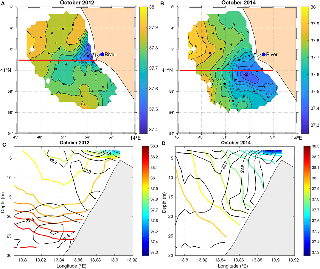
Figure 8. OA maps of salinity (g kg⁻¹) at 3 m (A,B) in October 2012 (left panel) and October 2014 (right panel). The fields are not plotted where the OA expected error exceeds 20%. The contour interval is 0.1 g kg⁻¹. Dots indicate location of stations. In (C,D), the vertical isolines of temperature (in black, contour interval 0.1°C in C and 0.05°C in D) and salinity (colored, contour interval 0.2 g kg⁻¹) are shown along the 41° 1'N and 41° N parallels (red lines), respectively.

These shape the horizontal and vertical distribution of salinity, especially during winter (Figure 9), when the surface river runoff increases strongly (Figure 6). In February 2013, the whole area is affected by transitional waters (Figure 9A). A wide and colder core (S~35.8 g kg⁻¹, T~13.1°C) is located in the northwestern side of the area, while the salinity increases southward and toward the coast (Figure 9A). In February 2014, the whole area is still affected by transitional waters (Figure 9B). The salinity presents lower values (S <36 g kg⁻¹) downstream along the coast and offshore, surrounding relatively saltier waters. The halocline is wider in February 2013 and shallower and steeper in February 2014 (Figures 9C,D), with convergent and divergent small areas toward the surface. The vertical profiles are gravitationally stable because the increase in temperature with depth is balanced by the progressive increase in salinity.

FIGURE 9

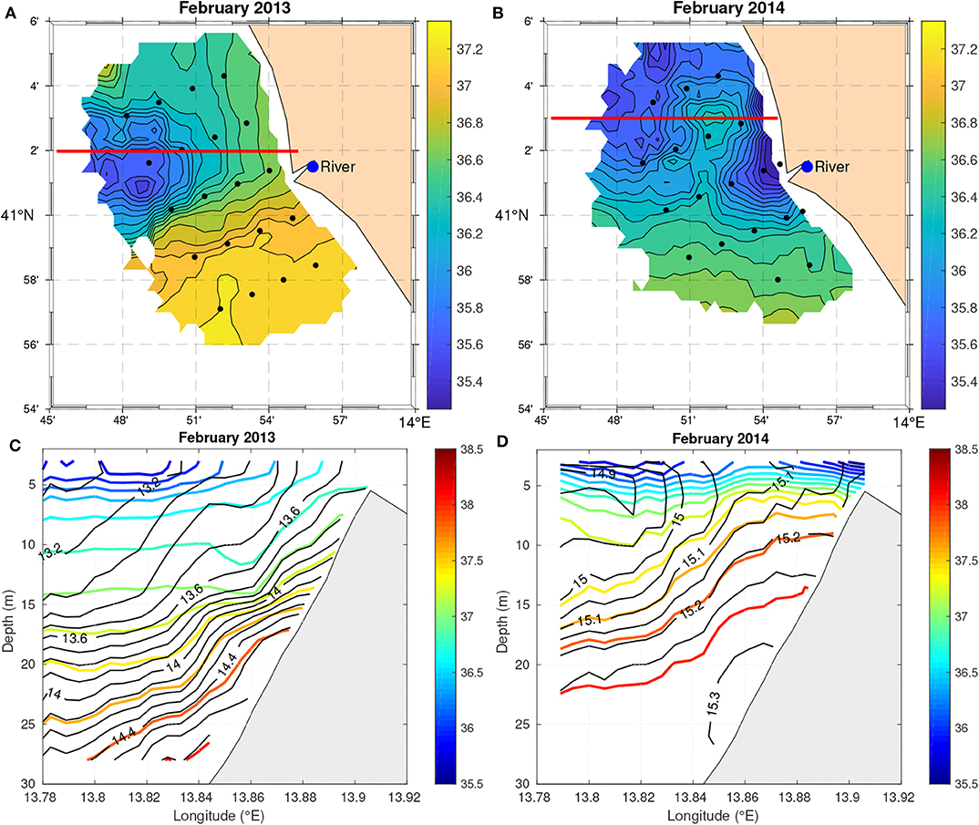
Figure 9. OA maps of salinity (g kg⁻¹) at 3 m (A,B) in February 2013 (left panel) and February 2014 (right panel). The fields are not plotted where the OA expected error exceeds 20%. The contour interval is 0.1 g kg⁻¹. Dots indicate location of stations. In (C,D), the vertical isolines of temperature (in black, contour interval 0.1°C in C and 0.05°C in D) and salinity (colored, contour interval 0.2 g kg⁻¹) are shown along the 41° 02'N and 41° 03'N parallels (red lines), respectively.

3.3. Steady Circulation Fields

Here, we describe the steady circulation at 5 m (below the Ekman surface layer) resulting from the diagnostic numerical experiments. The ocean model is initialized by the corresponding density field synoptically observed and optimally interpolated, as described in section 2.2. In order to establish a steady state of kinetic energy, the model is integrated for 10 days (Figure 10).

FIGURE 10

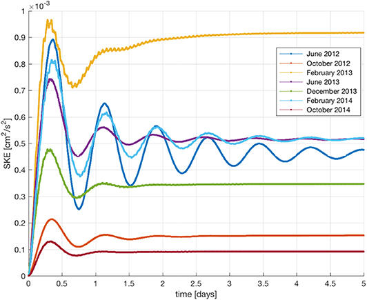
Figure 10. Surface Kinetic Energy time series for each survey during the first 5 days of time integration of the diagnostic calculation. Unit is cm²s⁻².

Low north-westerly winds and small horizontal density gradients determine a steady circulation characterized by a wide southern longshore current in June 2012 (Figure 11A). Maximum velocities (~8 cm s⁻¹) are detected along the coast in correspondence of the higher density gradients, especially close to the river mouth. This current separates the lighter waters offshore (σ_t~25.25 kg m⁻³) from the denser toward the coast (σ_t~25.75 kg m⁻³). The latter constrain the less dense transitional waters (σ_t~24.5 kg m⁻³) in the upper layer between the surface and 4 m depth (not shown). Along the water column, the velocity quickly decreases across the pycnocline, becoming zero below it.

FIGURE 11

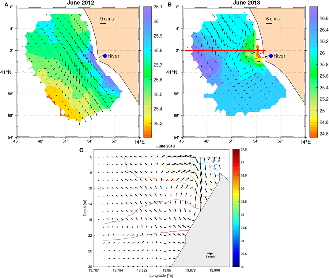
Figure 11. Density and steady circulation at 5 m from the diagnostic numerical experiment using temperature and salinity fields optimally interpolated from the CTDs of June 2012 (A) and in June 2013 (B). Units are kg m⁻³ for density (σ_t) and cm s⁻¹ for the total velocity, which are not plotted where the expected error of the OA on the observed temperature and salinity exceeds 20%. Panel (C) shows the vertical velocities and the density contours at 41° 02′ N (red line in B).

In June 2013, the density is strongly affected by the river outflow with the formation of a small lens of very light freshwater (σ_t~22 kg m⁻³) close to the river mouth (Figure 11B). Around this area, higher density gradients are detected, corresponding to a small-scale eddy whose dimension is ~10 km. This feature is represented by the model as a shallow (~15 m) anticyclonic recirculation cell (mainly baroclinic) and a downstream longshore current, favored by weak south-westerly winds. This eddy induces downwelling processes with a vertical velocity of ~8 mm s⁻¹ in the upper layer at about 10 m (Figure 11C). This dynamic condition is consistent with the downward deflection of the isopycnals (Figure 7D).

In autumn, the circulation is weak (Figure 10). In October 2012, the velocity field is dominated by a small-scale eddy located offshore and a southward longshore current (Figure 12A) induced by weak north-easterly winds. The model detects the eddy as the eastern side of a large anticyclone, whose horizontal dimension is comparable with the Rossby radius of deformation (~15 km). It preserves the less dense transitional waters at the surface (σ_t~ 26.24 kg m⁻³) from those surrounding them. The latter show relatively higher density values (σ_t~26.42 kg m⁻³) along the coast. This is due to the rising slope of the isohalines from 20 m depth toward the coast to the lowest limit of the halocline (Figure 8C). Here, the density is lower (σ_t~25.95 kg m⁻³), limited to a small area close to the river mouth.

FIGURE 12

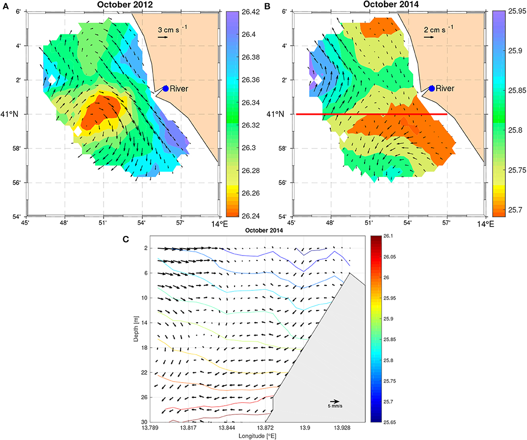
Figure 12. Density and steady circulation at 5 m from the diagnostic numerical experiment using temperature and salinity fields optimally interpolated from the CTDs of October 2012 (A) and in October 2014 (B). Units are kg m⁻³ for density (σ_t) and cm s⁻¹ for the total velocity, which are not plotted where the expected error of the OA on the observed temperature and salinity exceeds 20%. Panel (C) shows the vertical velocities and the density contours at 41° N (red line in B).

In October 2014, the wind is negligible, and the current field shows weak circulation, with higher velocities along the low density gradients in the north-western side of the domain (Figure 12B). These horizontal fronts approximately separate the denser saltier and warmer waters (σ_t~25.90 kg m⁻³) from the fresher and colder (σ_t~25.70 kg m⁻³), directly affected by the surface river runoff (Figure 6). As described in section 3.2, the temperature of the freshwater inflow destabilizes the vertical stratification of the water column and causes vertical mixing associated with weak downwelling processes. The model detects vertical velocities (Figure 12C) of about 1 mm s⁻¹, which significantly decrease below 10 m.

The steady velocity fields in February 2013 and 2014 are shown in Figure 13. The dynamic conditions in December 2013 are not described, as they are similar to those in February 2013. In such a period, the steady circulation is the most energetic (Figure 10). The velocity field is dominated by a relatively large anticyclonic structure, partially detected on the northern side of the domain (Figure 13A). Its dynamics preserve the relatively less dense water offshore (σ_t~27.2 kg m⁻³) from those surrounding it (σ_t~27.9 kg m⁻³). This feature is consistent with the slopes of the isotherms and isohalines (Figure 9C). Furthermore, it contributes to the southward current along the coast, also favored by weak northerly winds. Higher velocities of ~10 cm s⁻¹ are detected along the density front. The flow moves westward due to the constraint generated by the denser waters located in the south of the domain.

FIGURE 13

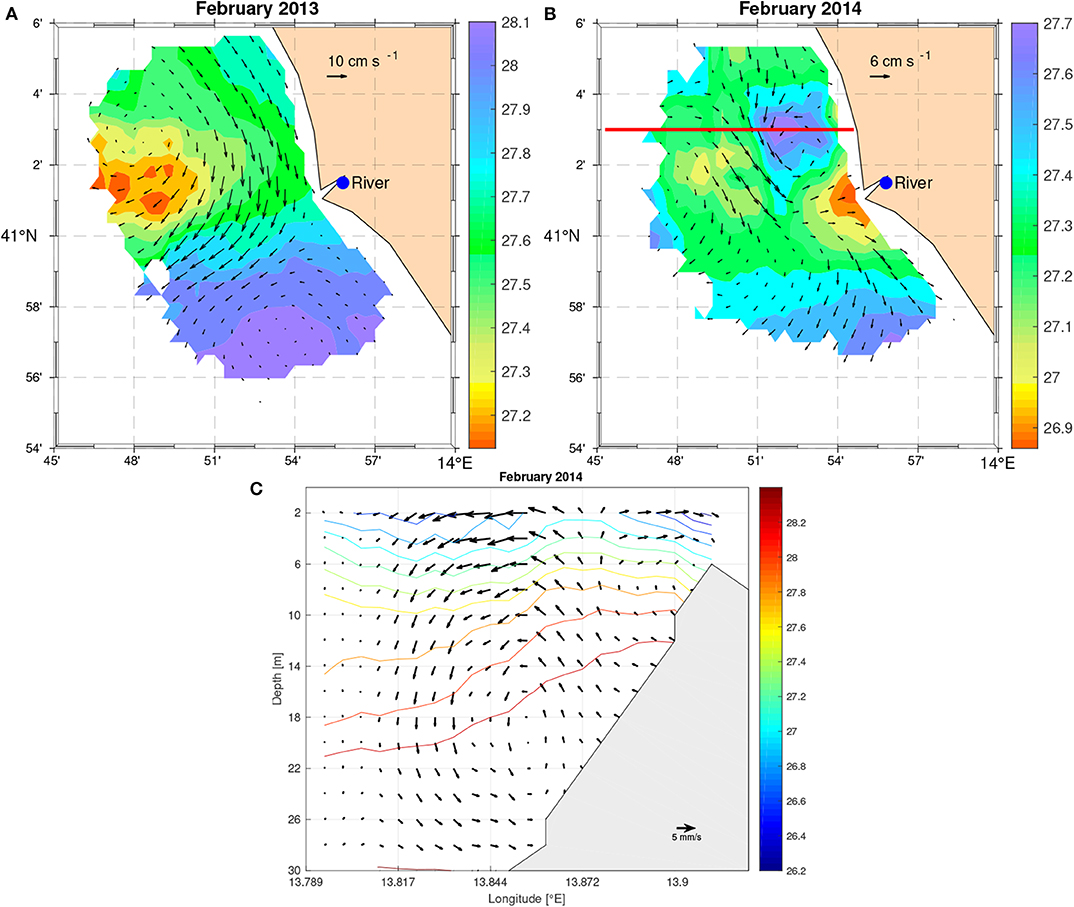
Figure 13. Density and steady circulation at 5 m from the diagnostic numerical experiment using temperature and salinity fields optimally interpolated from the CTDs of February 2013 (A) and in February 2014 (B). Units are kg m⁻³ for density (σ_t) and cm s⁻¹ for the total velocity, which are not plotted where the expected error of the OA on the observed temperature and salinity exceeds 20%. Panel (C) shows the vertical velocities and the density contours at 41° 03′ N (red line in B).

In February 2014, the total kinetic energy is lower (Figure 10) and the model gives a different steady dynamical condition (Figure 13B). The circulation is influenced by weak north-easterly winds and density gradients induced by the freshwater inflow from the higher surface river runoff (Figure 6). The velocity field is dominated by a wide and weak southerly current system (~5 cm s⁻¹), meandering around a small baroclinic cyclonic eddy. The model defines this feature as about 10 km in diameter and characterized by denser (saltier) waters (Figure 9B). The detection of this small-scale eddy is consistent with the slopes of the isotherms and isohalines shown in Figure 9D. The model detects the development of vertical velocities (Figure 13C), which induce an upwelling along the water column, increasing the salinity at the surface.

4. Summary and Conclusions

Seven CTD surveys were carried out between June 2012 and October 2014 in front of the Volturno river estuary in the Gulf of Gaeta (eastern Tyrrhenian Sea). During each survey, the area was synoptically sampled with 24 CTD casts in a nearly-regular grid (~2.5 km).

The data analyses show a density field dominated by strong temporal variability of the thermohaline properties, represented by three types of waters: freshwater of fluvial origin (S <34 g kg⁻¹), saltier water of Tyrrhenian origin (S > 37.8 g kg⁻¹), and transitional waters created through mixing of the previous two (34 < S <37.8 g kg⁻¹).

In early summer, the whole water column is characterized by a clear thermal stratification. The surfaces of discontinuity are predominantly horizontal, inducing conditions of strong vertical stability between the upper warmer waters and the colder and deeper saltier Tyrrhenian ones. This vertical condition inhibits the ventilation of the bottom layer and supports a weak horizontal dynamic. The stratification increases more in case of rainy events, like in June 2013, when a surface plume spreads over the coastal shelf along the direction of the Kelvin wave propagation. The model results identify this feature as a small baroclinic anticyclonic eddy that preserves a fresher water core at its center.

A neutral stratification occurs in autumn and winter. In autumn, the water column is characterized by a wide superficial mixed layer over a deeper thermocline, which reaches the bottom. In this layer, the temperature is higher than that in the early summer. Since there is no thermal gradient along the upper isothermal layer, the spatial density distribution is mainly determined by salinity, which shows higher values than in the early summer. Vice versa, toward the coast around the river mouth, the colder freshwater inflow destabilizes the vertical stratification, followed by the sinking of the transitional waters down to ~15 m. This is particularly evident in October 2014, when a wide river plume is observed slightly upstream.

In February 2014, a stratified salinity along the water column is evident, increasing in the upper layer due to the higher freshwater inflow. This preserves the vertical stability of the water column in the upper ~15 m, although the temperature profiles show a weak thermal inversion, with cooler waters floating above warmer. Such a destabilization of the water column is compensated by the salinity field. The bottom waters are not influenced by the transitional waters, retaining the accumulated heat. The upper ~6 m are characterized by transitional waters over the whole area, with a clear signal close to the river mouth and saltier water downstream. The model identifies this structure as a small-scale cyclonic eddy that induces convergence toward the surface. Although the surface river runoff in winter is higher, a clear river plume is not observed near the coast in February and December 2013. The observations show that the transitional waters mainly affect the northern side of the domain, across a relatively large anticyclonic eddy. This is a dynamical mechanism that preserves the transitional water core offshore.

In conclusion, this study provides evidence of the strong impact of the freshwater river inflow on the hydrological conditions at sea. This occurs in the upper layer, modifying the characteristics along the water column through the turbulent mixing processes. The transitional waters affect the whole study area, forming a horizontal layer whose thickness is strongly correlated to the seasonal vertical stratification and the surface river runoff. In particular, in October 2014, we observed reduced stability over the whole domain (Figure 4) and vertical instability occurring within the surrounding area close to the river mouth (not shown). Then, the thickness of the transitional waters increases, reaching its maximum depth of ~15 m. The waters and the coastal circulation are also modulated by meandering currents and small-scale eddies as detected by the diagnostic model. These structures modify the spatial distribution and the vertical stratification of the waters, preserving the transitional core from the saltier surrounding waters in the condition of anticyclonic circulation. The propagation of the anticyclonic eddies could be considered an important contribution to the transport of the transitional waters offshore.

The methodology described in this paper could also be used to analyze ocean data in order to respond to environmental emergencies, such as pollutant dispersion. The measured fields may also be used to determine the initial condition of the prognostic model, thus improving the forecast skill.

Data Availability Statement

The in-situ data used in this study are available in the SEANOE repository at: https://doi.org/10.17882/70324.

Author Contributions

RS and AD analyzed the results and wrote the paper. FP, AR, and AP analyzed the results and revised the paper. IA and SB analyzed the surface river runoff. LF, FL, and AC carried out CTD sampling. RS performed the numerical simulations. SB analyzed the wind fields. LF coordinated the research project I-AMICA.

Funding

This work has been funded by Project PON03 I-AMICA—High technology infrastructure for Climate-Environmental Integrated Monitoring (www.i-amica.it), Development Objective OR4.4—Study and monitoring of the interface processes between the biosphere, hydrosphere, and functionality of coastal ecosystems.

Conflict of Interest

The authors declare that the research was conducted in the absence of any commercial or financial relationships that could be construed as a potential conflict of interest.

Acknowledgments

We thank the captains and the crews of the R/V Astrea for their support in CTD data acquisition during the surveys mentioned in the article. Data are freely available at the SEANOE repository at the following link: https://www.seanoe.org/data/00591/70324/.

References

Astraldi, M., and Gasparini, G. P. (1994). The seasonal characteristics of the circulation in the Tyrrhenian sea, in seasonal and interannual variability of the western Mediterranean sea. Coast. Estuar. Stud. 46, 115–134. doi: 10.1029/CE046p0115

CrossRef Full Text | Google Scholar

Bainbridge, Z. T., Wolanski, E., Álvarez Romero, J. G., Lewis, S. E., and Brodie, J. E. (2012). Fine sediment and nutrient dynamics related to particle size and floc formation in a Burdekin river flood plume, Australia. Mar. Pollut. Bull. 65, 236–248. doi: 10.1016/j.marpolbul.2012.01.043

PubMed Abstract | CrossRef Full Text | Google Scholar

Blumberg, A. F., and Mellor, G. L. (2013). “A description of a three-dimensional coastal ocean circulation model,” in Three-Dimensional Coastal Ocean Models, ed N.S. Heaps. doi: 10.1029/CO004p0001

CrossRef Full Text | Google Scholar

Bonomo, S., Cascella, A., Alberico, I., Lirer, F., Vallefuoco, M., Marsella, E., et al. (2018). Living and thanatocoenosis coccolithophore communities in a neritic area of the central Tyrrhenian Sea. Marine Micropalenontology 142, 67–91. doi: 10.1016/j.marmicro.2018.06.003

CrossRef Full Text | Google Scholar

Bretherton, F. P., Davis, R. E., and Fandry, C. (1976). A technique for objective analysis and design of oceanographic experiments applied to mode-73. Deep Sea Res. Oceanogr. Abstr. 23, 559–582. doi: 10.1016/0011-7471(76)90001-2

CrossRef Full Text | Google Scholar

Budillon, G., and Pierini, Sansone, Spezie (1999). Caratteristiche idrodinamiche lungo la fascia costiera campano-laziale. Ann. Facol. Sci. Nautiche 64, 7–17.

Carter, E. F., and Robinson, A. R. (1979). Analysis models for the estimation of oceanic fields. J. Atmos. Ocean. Technol. 4, 49–74. doi: 10.1175/1520-0426(1987)004<0049:AMFTEO>2.0.CO;2

CrossRef Full Text | Google Scholar

Chapman, D. C., and Lentz, S. J. (1994). Trapping of a coastal density front by the bottom boundary layer. J. Phys. Oceanogr. 24, 1464–1479. doi: 10.1175/1520-0485(1994)024<1464:TOACDF>2.0.CO;2

CrossRef Full Text | Google Scholar

Chelton, D. B., deSzoeke, R. A., Schlax, M. G., El Naggar, K., and Siwertz, N. (1998). Geographical variability of the first baroclinic rossby radius of deformation. J. Phys. Oceanogr. 28, 433–460. doi: 10.1175/1520-0485(1998)028<0433:GVOTFB>2.0.CO;2

CrossRef Full Text | Google Scholar

Cocco, E., and Pippo, T. D. (1988). Tendenze evolutive e dinamiche delle spiagge della campania e della lucania. Mem. Soc. Geol. It. 41, 195–204.

Google Scholar

Cole, K. L., and Hetland, R. D. (2016). The effects of rotation and river discharge on net mixing in small-mouth kelvin number plumes. J. Phys. Oceanogr. 46, 1421–1436. doi: 10.1175/JPO-D-13-0271.1

CrossRef Full Text | Google Scholar

De Pippo, T., Donadio, C., and Pennetta, M. (2003). Morphological control on sediment dispersal along the southern Tyrrhenian coastal zones (Italy). Geol. Romana 37, 113–121.

Google Scholar

Devlin, M. J., McKinna, L. W., Álvarez-Romero, J. G., Petus, C., Abott, B., Harkness, P., et al. (2012). Mapping the pollutants in surface riverine flood plume waters in the great barrier reef, Australia. Mar. Pollut. Bull. 65, 224–235. doi: 10.1016/j.marpolbul.2012.03.001

PubMed Abstract | CrossRef Full Text | Google Scholar

Ezer, T., Ko, D. S., and Mellor, G. L. (1992). Modelling and forecasting the Gulf stream. Mar. Technol. Soc. 26, 5–14.

Google Scholar

Ezer, T., and Mellor, G. L. (1992). A numerical study of the variability and the separation of the Gulf stream induced by surface atmospheric forcing and lateral boundary flows. J. Phys. Oceanogr. 22, 660–682. doi: 10.1175/1520-0485(1992)022<0660:ANSOTV>2.0.CO;2

CrossRef Full Text | Google Scholar

Ezer, T., and Mellor, G. L. (1994). Diagnostic and prognostic calculations of the north Atlantic circulation and sea level using a sigma coordinate ocean model. J. Geophys. Res. Oceans 99, 14159–14171. doi: 10.1029/94JC00859

CrossRef Full Text | Google Scholar

Ezer, T., Mellor, G. L., Ko, D., and Sirkes, Z. (1993). A comparison of Gulf stream sea surface height fields derived from geosat altimeter data and those derived from sea surface temperature data. J. Atmos. Ocean. Technol. 10, 76–87. doi: 10.1175/1520-0426(1993)010<0076:ACOGSS>2.0.CO;2

CrossRef Full Text | Google Scholar

Ferrara, C., Lega, M., Fusco, G., Bishop, P., and Endreny, T. (2017). Characterization of terrestrial discharges into coastal waters with thermal imagery from a hierarchical monitoring prpgram. Water 9, 1–14. doi: 10.3390/w9070500

CrossRef Full Text | Google Scholar

Ferraro, L., Bonomo, S., Alberico, I., Cascella, A., Giordano, L., Lirer, F., et al. (2018). Live benthic foraminifera from the Volturno river mouth (central Tyrrhenian Sea, Italy). Rend. Fis. Acc. Lincei. 29, 559–570. doi: 10.1007/s12210-018-0712-9

CrossRef Full Text | Google Scholar

Fong, D. A., and Geyer, W. R. (2001). Response of a river plume during an upwelling favorable wind event. J. Geophys. Res. Oceans 106, 1067–1084. doi: 10.1029/2000JC900134

CrossRef Full Text | Google Scholar

Fong, D. A., and Geyer, W. R. (2002). The alongshore transport of freshwater in a surface-trapped river plume. J. Phys. Oceanogr. 32, 957–972. doi: 10.1175/1520-0485(2002)032<0957:TATOFI>2.0.CO;2

CrossRef Full Text | Google Scholar

Fratianni, C., Pinardi, N., Lalli, F., Simoncelli, S., Coppini, G., Pesarino, V., et al. (2016). Operational oceanography for the marine strategy framework directive: the case of the mixing indicator. J. Oper. Oceanogr. 9(Suppl. 1):s223–33. doi: 10.1080/1755876X.2015.1115634

CrossRef Full Text | Google Scholar

Gan, J., Li, L., Wang, D., and Guo, X. (2009). Interaction of a river plume with coastal upwelling in the northeastern south China sea. Continent. Shelf Res. 29, 728–740. doi: 10.1016/j.csr.2008.12.002

CrossRef Full Text | Google Scholar

Garvine, R. W. (1999). Penetration of buoyant coastal discharge onto the continental shelf: a numerical study. J. Phys. Oceanogr. 29, 1892–1909. doi: 10.1175/1520-0485(1999)029<1892:POBCDO>2.0.CO;2

CrossRef Full Text | Google Scholar

Garvine, R. W. (2001). The impact of model configuration in studies of buoyant coastal discharge. J. Mar. Res. 59, 193–225. doi: 10.1357/002224001762882637

CrossRef Full Text | Google Scholar

Gill, A. E. (1982). Atmosphere-Ocean Dynamic. Academic Press. 30, 1–662.

Hellerman, S., and Rosenstein, M. (1983). Normal monthly wind stress over the world ocean with error estimates. J. Phys. Oceanogr. 13, 1093–1104. doi: 10.1175/1520-0485(1983)013<1093:NMWSOT>2.0.CO;2

CrossRef Full Text | Google Scholar

Hetland, R. D. (2005). Relating river plume structure to vertical mixing. J. Phys. Oceanogr. 35, 1667–1688. doi: 10.1175/JPO2774.1

CrossRef Full Text | Google Scholar

Hetland, R. D. (2010). The effects of mixing and spreading on density in near-field river plumes. Dyn. Atmos. Oceans 49, 37–53. doi: 10.1016/j.dynatmoce.2008.11.003

CrossRef Full Text | Google Scholar

Hetland, R. D., and Signell, R. P. (2005). Modeling coastal current transport in the gulf of maine. Deep Sea Res. II 52, 2430–2449. doi: 10.1016/j.dsr2.2005.06.024

CrossRef Full Text | Google Scholar

Hopkins, T. (1988). Recent observations on the intermediate and deep water circulation in the southern Tyrrhenian sea. Oceanol. Acta 9, 41–50.

Google Scholar

Hordoir, R., Nguyen, K. D., and Polcher, J. (2006). Simulating tropical river plumes, a set of parametrizations based on macroscale data: a test case in the Mekong delta region. J. Geophys. Res. Oceans 111:C09036. doi: 10.1029/2005JC003392

CrossRef Full Text | Google Scholar

Horner-Devine, A. R., Hetland, R. D., and MacDonald, D. G. (2015). Mixing and transport in coastal river plumes. Annu. Rev. Fluid Mech. 47, 569–594. doi: 10.1146/annurev-fluid-010313-141408

CrossRef Full Text | Google Scholar

Iermano, I., Liguori, G., Iudicone, D., Giordano Nardelli, B., Colella, S., Zingone, A., et al. (2012). Filament formation and evolution in buoyant coastal waters: observation and modelling. Progr. Oceanogr. 106, 118–137. doi: 10.1016/j.pocean.2012.08.003

CrossRef Full Text | Google Scholar

Kelsey-Wilkinson, D. (2014). Assessing the impact of seasonal variations on the density structure of a weak freshwater plume. Plymouth Student Sci. 7, 14–31.

Google Scholar

MacDonald, D. G., Carlson, J., and Goodman, L. (2013). On the heterogeneity of stratified-shear turbulence: Observations from a near-field river plume. J. Geophys. Res. Oceans 118, 6223–6237. doi: 10.1002/2013JC008891

CrossRef Full Text | Google Scholar

MacDonald, D. G., and Geyer, W. R. (2005). Hydraulic control of a highly stratified estuarine front. J. Phys. Oceanogr. 35, 374–387. doi: 10.1175/JPO-2692.1

CrossRef Full Text | Google Scholar

Mancini, L., Cero, C. D., Gucci, P., Venturi, L., Carlo, M. D., and Volterra, L. (1994). Il fiume Volturno-la definizione dello stato di salute del corpo idrico. Inquinamento 10, 70–83.

Google Scholar

Mangoni, O., Aiello, G., Balbi, S., Barra, D., Bolinesi, F., Donadio, C., et al. (2016). A multidisciplinary approach for the characterization of the coastal marine ecosystems of Monte di Procida (Campania, Italy). Mar. Pollut. Bull. 112, 443–451. doi: 10.1016/j.marpolbul.2016.07.008

PubMed Abstract | CrossRef Full Text | Google Scholar

McCabe, R. M., MacCready, P., and Hickey, B. M. (2009). Ebb-tide dynamics and spreading of a large river plume. J. Phys. Oceanogr. 39, 2839–2856. doi: 10.1175/2009JPO4061.1

CrossRef Full Text | Google Scholar

McLusky, D. S., and Elliott, M. (2004). The Estuarine Ecosystem. Threats and Management. Oxford: Oxford University Press, 216. doi: 10.1093/acprof:oso/9780198525080.001.0001

CrossRef Full Text | Google Scholar

Mellor, G. (1991). An equation of state for numerical models of oceans and estuaries. J. Atmos. Ocean. Technol. 8, 8609–611. doi: 10.1175/1520-0426(1991)008<0609:AEOSFN>2.0.CO;2

CrossRef Full Text | Google Scholar

Mellor, G., and Yamada, T. (1982). Development of a turbulence closure model for geophysical fluid problems. Rev. Geophys. Space Phys. 20, 851–875. doi: 10.1029/RG020i004p00851

CrossRef Full Text | Google Scholar

Mellor, G. L., and T. Ezer, L. Y. O. (1994). The pressure gradient conundrum of sigma coordinate ocean models. J. Atmos. Ocean. Technol. 11, 1126–1134. doi: 10.1175/1520-0426(1994)011<1126:TPGCOS>2.0.CO;2

CrossRef Full Text | Google Scholar

Moretti, M., Sansone, E., Spezie, G., Vultaggio, M., and De Maio, A. (1977). Alcuni aspetti del movimento delle acque del Golfo di Napoli. Annali IUN 45–46:207–217.

Nekouee, N., Hamidi, S., J. W. Roberts, P., and Schwab, D. (2015). Assessment of a 3D hydrostatic model (POM) in the near field of a buoyant river plume in Lake Michigan. Water Air Soil Pollut. 226:210. doi: 10.1007/s11270-015-2488-1

CrossRef Full Text | Google Scholar

Nurser, A. J. G., and Bacon, S. (2014). The rossby radius in the Arctic Ocean. Ocean Sci. 10, 967–975. doi: 10.5194/os-10-967-2014

CrossRef Full Text | Google Scholar

Onken, R., Robinson, A. R., Kantha, L., Lozano, C. J., and P. J. Haley, S. C. (2005). A rapid response nowcast/forecast system using multiply nested ocean models and distributed data systems. J. Mar. Syst. 56, 45–66. doi: 10.1016/j.jmarsys.2004.09.010

CrossRef Full Text | Google Scholar

Onken, R., and Sellschopp, J. (2001). Water masses and circulation between the Eastern Algerian Basin and the Strait of Sicily in October 1996. Oceanol. Acta 24, 151–166. doi: 10.1016/S0399-1784(00)01135-X

CrossRef Full Text | Google Scholar

Osadchiev, A., and Korshenko, E. (2017). Small river plumes off the northeastern coast of the black sea under average climatic and flooding discharge conditions. Ocean Sci. 13, 465–482. doi: 10.5194/os-13-465-2017

CrossRef Full Text | Google Scholar

Osborn, T. R. (1980). Estimates of the local rate of vertical diffusion from dissipation measurements. J. Phys. Oceanogr. 10, 83–89. doi: 10.1175/1520-0485(1980)010<0083:EOTLRO>2.0.CO;2

CrossRef Full Text | Google Scholar

Parrella, A., Isidori, M., Lavorgna, M., and Dell'Aquila, A. (2003). Stato di qualita del fiume volturno integrato da indagini di tossicita e genotossicita. Ann Ig 15, 147–157.

PubMed Abstract | Google Scholar

Ribotti, A., Bonomo, S., Alberico, I., Lirer, F., Cascella, A., Ferraro, L., et al. (2019). I-amica coastal hydrological surveys in the eastern tyrrhenian sea. SEANOE repository. doi: 10.17882/70324

CrossRef Full Text | Google Scholar

Robinson, A. R., and Golnaraghi, M. (1993). Circulation and dynamics of the eastern Mediterranean Sea: quasi synoptic data driven simulations. Deep Sea Res. 40, 1207–1246. doi: 10.1016/0967-0645(93)90068-X

CrossRef Full Text | Google Scholar

Sorgente, R., Tedesco, C., Pessini, F., De Dominicis, M., Gerin, R., Olita, A., et al. (2016). Forecast of drifter trajectories using a rapid environmental assessment based on CTD observations. Deep Sea Res. II 133, 39–53. doi: 10.1016/j.dsr2.2016.06.020

CrossRef Full Text | Google Scholar

Thiebaux, J., and Pedder, M. A. (1988). Spatial objective analysis with applications in atmosphere science. Q. J. R. Meteorol. Soc. 114, 553–554. doi: 10.1002/qj.49711448017

CrossRef Full Text | Google Scholar

Wong, L., Chen, J., and Dong, L. (2004). A model of the plume front of the pearl river estuary, China and adjacent coastal waters in the winter dry season. Continent. Shelf Res. 24, 1779–1795. doi: 10.1016/j.csr.2004.06.007

CrossRef Full Text | Google Scholar

Wright, L. D. (1977). Sediment transport and deposition at river mouths: a synthesis. GSA Bull. 88, 857–868. doi: 10.1130/0016-7606(1977)88<857:STADAR>2.0.CO;2

CrossRef Full Text | Google Scholar

Zavatarelli, M., Pinardi, N., Kourafalou, V. H., and Maggiore, A. (2002). Diagnostic and prognostic model studies of the Adriatic sea general circulation: seasonal variability. J. Geophys. Res. Oceans 107, 2-1–2-20. doi: 10.1029/2000JC000210

CrossRef Full Text | Google Scholar