A Study of Circulation, Turbulence, and Tidal Stream Resources in the Taiwan Strait

Introduction

As interest in renewable marine energy increases, the number of investigations of tidal currents and analyses of their properties is growing. Understanding these properties enables the identification of prospective sites where tidal energy converters (TECs) will be most efficient. Although it is not the only means of assessing potential sites for deploying tidal turbines, the most popular method is numerical simulations of water circulation and inferring the turbulence characteristics and power density from model outputs.

Tidal energy site resource assessment studies are usually performed to obtain valuable data and analyses that will help in formulating and improving tidal energy site resource assessment practices, while also adding to our knowledge of hydrodynamic conditions at tidal energy sites (Goddijn-Murphy et al., 2012; Polagye and Thomson, 2013; Milne et al., 2013; Gunawan et al., 2014). Selecting potential sites for tidal energy projects involves more than simply identifying sites with an appropriately large peak tidal current (Bryden and Couch, 2006), and site selection for TEC arrays consists of various practical and economic constraints, such as magnitude and other properties of the tidal forcing, water depths appropriate for the chosen technology, and navigational constraints (Couch and Bryden, 2006; Iglesias et al., 2012).

The most suitable tidal stream sites are usually located in relatively shallow waters along the continental shelf where tidal currents are greatly enhanced. However, in shallow water, TECs may be subject to the effects of wind-generated surface-gravity waves, because in stormy conditions the magnitude of the velocity fluctuations can reach the same magnitude as those of the operating range of the turbine (Milne et al., 2013). Extreme loads experienced in such conditions are likely to constrain the proximity of a turbine to the surface with respect to the efficiency of tidal energy conversion.

From a resource and device perspective, it is more beneficial to select sites with tidal symmetry, i.e., those where the tidal currents have an equal magnitude during the ebb and flood phases. Symmetrical sites are also good, as similar levels of energy generation can be achieved during both flood and ebb phases. Sites with either flood- or ebb-dominance, i.e., those manifesting tidal asymmetry, are less suitable for exploitation because tidal turbines mounted there could have a greater environmental impact on the seafloor, coastline erosion, and sediment transport than those in symmetrical sites (Neill et al., 2009).

Turbulence can also have a significant impact on tidal turbine effectiveness, which should be investigated when assessing site resources. Of the various turbulence quantities, streamwise turbulence intensity is generally regarded as the turbulence parameter most relevant to unsteady loading on tidal turbines, as it can cause the failure of and even damage them (McCann et al., 2008). Quantifying the turbulence intensity has thus been the focus of the majority of recent efforts to measure tidal energy sites that have provided valuable new observations of turbulence intensity at various elevations from the seabed in relatively fast flows for a variety of channel configurations (Milne et al., 2016).

The Taiwan Strait (TS) is a water body with a high potential for tidal energy conversion, as tidal stream sites suitable for mounting tidal converters are located in relatively shallow waters where tidal currents are significantly enhanced (Chen et al., 2013). However, mounting a turbine close to the bottom can cause certain difficulties. The interaction of the bottom boundary layer (BBL) with tidal flow produces intense turbulence (called wall-bounded turbulence) due to bottom drag (Rippeth et al., 2002; Korotenko et al., 2013). Along with the coherent structures near the bottom (Thomson et al., 2010; McCaffrey et al., 2015), wall-bounded turbulence may also greatly reduce the efficiency of TECs mounted so low.

Although there have been numerous observational and modeling studies of circulation in the TS, no studies have specifically sought to identify the optimum locations and details for the prospective deployment of convertors in the entire Strait. The objective of this paper is, therefore, to fill this gap by identifying potentially suitable sites for tidal stream energy conversion. To our knowledge, the present study is the first attempt to assess the tidal power potential of the entire TS.

In this work, we used the 3-D Princeton Ocean Model (POM) with tidal forcing driven by a 2-D barotropic model to examine the time-depth variability of tidal currents and turbulence and to evaluate the power density in the TS. The paper is organized as follows: In section “Materials and Methods,” we describe the study region, the formulation and implementation of the model, its forcing and boundary conditions, and bottom topography. Our results are presented and discussed in section “Results and Discussion,” which includes an evaluation of model predictions, simulated water elevation, and a description of the structure of horizontal velocity. In section “Tidal Turbulence in the Peng-Hu Channel,” the time-depth variability of tidal velocity and turbulent diffusivity in the Peng-Hu Channel (PHC) is evaluated. The power density estimates obtained at zonal and meridional sections are discussed in section “Power Density Assessment,” and the summary and conclusion are presented in section “Summary and Conclusion.”

Materials and Methods

Study Region

The TS is a shallow passage about 200 km wide between the Chinese mainland and the island of Taiwan, connecting the South China Sea in the south and the East China Sea in the north. Figure 1 shows the TS’s bathymetry and the surrounding areas at its northern and southern edges. Most of the strait is shallower than 80 m. The major topographic features of the TS are the Taiwan Bank in the southwest, the Chang-Yuen Rise (CYR) north of the narrow PHC located between the Taiwan Island, and the Peng-Hu (PH) Archipelago. This channel is the major southern deep passage and a prime gate to the TS (Jan et al., 1994, 2010).

FIGURE 1

Figure 1. Bathymetry of the Taiwan Strait. Solid horizontal (ZS1–3) and vertical (MS1–3) lines denote zonal and meridional exploratory sections for power density assessment. Numbers 1 and 2 denote Zhuoshui and Wu river’s estuaries. The asterisk F denotes the site of the hydrographic survey. Letters A–D indicate the sites of turbulent diffusivity estimates (see section Tidal Turbulence in the Peng-Hu Channel). CYR, Chang-Yuen Ridge; PH, Peng-Hu Archipelago; PHC, Peng-Hu Channel; and TB, Taiwan Bank (modified from Jan and Chao, 2003).

East of the PH Archipelago, the wedge-like PHC is about 50 km wide. Ascending northward sharply from deeper than 1,000 to 70 m, the PHC merges with the southern flank of the CYR, a significant topographic feature of the TS. The CYR, a shallow, sandy submarine ridge, is characterized by a very gentle bottom slope. A considerable part of the CYR is subject to drying and inundation during the tidal cycle. Being stretched west from the central part of the western coast of the island of Taiwan (Figure 1), the CYR is known to be a barrier for dense water flowing from the PHC, so that the heavier water impinging on the CYR turns northwestward in front of the ridge. Lighter surface waters tend to be distributed along the eastern side of the TS and flow over the CYR (Jan et al., 1994, 2002); the velocity magnitude is greatly enhanced during the flood and ebb, with peaks exceeding 2.5 m s^–1 during the spring tide.

Semidiurnal tidal oscillations play a crucial role in the circulation of the TS (Chuang, 1985, 1986; Jan et al., 2002). The tide enters the TS through the northern and southern openings, and then converges in the central part of the strait. Most of the energy of the semidiurnal tide comes from the north. It has been suggested that both standing (Lin et al., 2000) and propagating (Jan et al., 2002) semidiurnal tides coexist in the TS. The diurnal tide in the TS is less intense than the semidiurnal tide, except in the southernmost sector. As sea level measurements revealed, the diurnal tide propagates from north to south (Hwung et al., 1986).

Model Formulation and Application

A 1-min (e.g., 1 nautical mile) resolution σ-coordinate 3-D primitive equation POM was used to study the tidal circulation and assess the energy of tidal currents in the TS. We applied the hydrostatic version of the POM (Blumberg and Mellor, 1987) with a level 2.5 M–Y turbulence closure (Mellor and Yamada, 1982) that solves full thermodynamic equations of motion. A detailed description of the model can be found at http://jes.apl.washington.edu/modsims_two/usersguide0604.pdf.

The POM grid area covers most of the TS from 23°N to 25°N and from 116.5°E to 121.0°E (Figure 1). The model domain was divided into 270 × 122 grid cells corresponding to a meridional resolution of 1.836 km and a zonal resolution ranging from 1.723 km at 23°N to 1.698 km at 25°N. On the z-axis, unevenly distributed 21 σ-levels were adopted to provide higher resolution near the surface and bottom. The minimum water depth in the model domain was set to 5 m.

To simulate the tidal currents in the TS, the POM was initialized with monthly averaged temperature and salinity fields at standard depth levels (Levitus, 2009) interpolated to the POM σ-levels. During the 1-month spin-up period the model was forced with tidal forcing; once this period was complete the model was forced with both tidal and river forcing (see section “River Forcing” for further details). To ensure numerical stability, the model was run with an external mode time step of 30 s and an internal mode time step of 120 s.

Vertical Boundary Conditions

Stress components at the free surface, ${\mathrm{\tau }}_s^x$ and ${\mathrm{\tau }}_s^y$ are described as

$$({\mathrm{\tau }}_s^x,{\mathrm{\tau }}_s^y)=(<wu>,<wv>)(1)$$

where < wu > and < wv > are average surface (kinematic) wind stress components. The bottom stress components, ${\mathrm{\tau }}_b^x$ and ${\mathrm{\tau }}_b^y$ induced by bottom friction are described as

$$({\mathrm{\tau }}_b^x,{\mathrm{\tau }}_b^y)=C_z{(U^2+V^2)}^{1/2}(U,V)(2)$$

where U and V are horizontal velocity components, C_z is the non-dimensional coefficient (which is a function of the roughness length of the bed, z₀), and the water depth is H:

$$C_z=\text{MAX}(\frac{{\mathrm{\kappa }}^2}{{\left\{ln\left[\frac{\left(1+{\mathrm{\sigma }}_{kb-1}\right)H}{z_0}\right]\right\}}^2},\mathrm{\hspace{0.17em}\hspace{0.33em}0.0025})\mathit{\hspace{1em}\hspace{1em}\hspace{1em}\hspace{1em}\hspace{1em}\hspace{1em}\hspace{1em}\hspace{1em}\hspace{0.5em}\hspace{1em}}(2a)$$

where σ_kb–1is the depth of the layer overlying the bottom one in sigma coordinates and κ = 0.4 is the von Kármán constant. In other words, the bottom friction is determined by the current velocity of the layer nearest to the bed, where a logarithmic current profile is assumed, and the bottom friction is determined by the current speed of the layer nearest to the seabed. However, in the oscillatory boundary layer flow, velocity profiles near the seabed may deviate from logarithmic profiles. Using numerical experiments, Kuo et al. (1996) showed that even small deviations from logarithmic profiles will result in significant errors when the profiles are used to calculate the bed roughness length and shear stress, especially when the steep irregular bathymetry is calculated for. To avoid this drawback for the shallow region as the TS, instead of Eq. (2a) we used the Manning formula to parameterize the bottom friction (Liu et al., 2003; Chiou et al., 2010): i.e., C_z = g/(nH^−1/6)², where n is the Manning coefficient and g is the acceleration of gravity. Here, the bottom friction is calculated from the current velocity U and V averaged over the water depth, along with the coefficient n at the corresponding location. In this case, the depth-averaged velocity is much less sensitive to the logarithmic profile assumption used in conventional parameterizations for C_z. Following Chiou et al. (2010), we set the Manning coefficient n for the TS as 0.032 s m^–1/3.

Open Boundary Conditions and Tidal Forcing

The model domain is presented in Figure 2. It reproduces all of the major topographic features of the TS described in section “Study Region.” The western section of the TS is shallow (about ∼ 50 m deep) with the bottom sloping gently toward the center. In contrast, the eastern shore of the Strait has an abrupt bottom topography with the deep PHC in the south and the sandy CYR stretching offshore in the middle. The depth at the top of the CYR is about 15 m. Beyond the CYR, numerous local elevations irregularly cover the bottom of the TS. Their heights are comparable to that of the CYR.

FIGURE 2

Figure 2. The 3-D model domain with 1 nautical min grid, showing the model’s horizontal resolution with numerous islands, channels, and complex bottom topography features. The x-axis denotes East-West direction; the y-axis denotes North-South direction. CYR, PH, PHC, and points 1 and 2 are defined in Figure 1. S_b and N_b represent the southern and northern open boundaries, respectively (modified from Korotenko et al., 2014).

The model was driven by spatial variance along the open boundaries of the sea surface heights and meridional velocities specified at the two open ends at the south and north. The zonal boundary velocities were not used for two reasons: (1) these velocities are relatively small compared to the meridional ones; and (2) to avoid numerical instability (which occurred mostly around small islands near the south boundary of the western coast) of the POM utilizing the 1-min horizontal grid. The temporal resolution of the tidal forcing data supplied by BTM was 20 min, adequately resolving the tidal cycle.

The southern (S_b) and northern (N_b) open boundaries are shown in Figure 2. At these boundaries, the inflow and outflow types of conditions were set for temperature and salinity. In the case of the inflow into the domain, the values of T and S were set at the corresponding open boundary, while in the case of the outflow from the domain, the radiation condition

$$\frac{\partial }{\partial t}(T,S)+{\overline{U}}_n\frac{\partial }{\partial n}(T,S)=0(3)$$

was used. The index n represents the direction normal to the open boundary and ${\overline{U}}_n$ is the vertically averaged normal component of the velocity.

The vertically averaged (barotropic) velocities on the open boundaries were estimated using Flather’s (1976) formula:

$${\overline{U}}_n={\overline{U}}_n^o+\sqrt{\frac{g}{H}}\left(\mathrm{\eta }-{\mathrm{\eta }}_0\right)(4)$$

where η₀ and ${\overline{U}}_n^o$ were the sea surface elevation and the vertically averaged normal component of barotropic velocity, respectively, provided by the tidal model at the corresponding open boundary; ${\overline{U}}_n$ is the barotropic velocity at the corresponding open boundary at time t; η is the model sea surface elevation calculated from the continuity.

For tidal forcing, we used data from a 1/12° Barotropic Tidal Model (BTM) for the TS, kindly provided by J.-Y. Liou¹ (personal communication). The BTW was designed to examine the characteristics of barotropic tides and to predict tidal sea levels and currents in the seas around Taiwan. The model grid covers the area from 18°N to 30°N and from 110°E to 130°E. In the model, harmonic constants of eight principal tidal constituents known for TS (S2, N2, K2, K1, O1, P1, Q1, and M4) were calculated and validated. The main result obtained with the model was that the semi-diurnal tide consists of two branches that enter the TS from the south and north, respectively. The north branch is a degenerative rotary tidal system that converges with the south branch in the middle of the TS. A description of the BTM is given by Zhu et al. (2009). The open boundary conditions S_b and N_b were obtained from the BTM by interpolation of velocities and water elevation at corresponding latitudes (Figure 2).

The tidal data corresponds to the period of transition of the tide from the neap to spring phase (June 25–30, 2013). During that period, tidal data indicated the surface elevation at relatively sea level and meridional velocity at the northern boundary ranged from approximately 2 m and 0.5 m s^–1 on the flood to approximately −2.8 m and −0.5 m s^–1 on the ebb, respectively. At the southern boundary, the surface elevation and meridional velocity ranged from about 1.2 m and 0.8 m s^–1 at the flood to about −1.2 m and −1.5 m s^–1 at the ebb, respectively. An examination of the sea surface elevation and meridional velocity at the boundaries revealed that they varied with the dominant semidiurnal (M2) constituent, although other harmonics disturbed the dominant M2 cycle only slightly.

Wind Forcing

The surface boundary condition (1) requires data on the surface wind stress components. The period June 25–30, 2013, as indicate NCEP/NCAR² data and our measurements (see Appendix), has characterized by weak northeasterly winds (<5 ms^–1) over the TS. Such winds are unlikely to produce a negligible effect on tidal current. To control the latter, further, we run the model without wind forcing, i.e., < wu > = < wv > = 0. Effects of strong wind and waves on tidal currents and power density one can find in numerous papers (c.f. Norris and Droniou, 2007; Milne et al., 2013; Korotenko and Sentchev, 2019).

River Forcing

River forcing was imposed as follows. After the initial spin-up period (one month) with tidal forcing, the POM model was forced with discharges of two rivers, the Zhuoshui and the Wu. The locations of the river estuaries are depicted in Figure 1. The river input was specified by the vertical velocity at the sea surface, w_S, which was imposed at the corresponding model grid points. We assumed that w_S injects volume and freshwater (salinity = 0), but no momentum. Following Oey (1996), w_S was defined as w_S = −Q/(NΔxΔy), where Q is the river discharge rate (m³ s^–1) and N is the number of grid areas covering the river mouth. In the model, the discharge rates for the Zhuoshui and Wu Rivers were set to the mean climatic values for the summer, equaling 220 and 60 m³ s^–1, respectively (Korotenko et al., 2014).

To stabilize the river plume sizes, the model was run with both tidal forcing and a seamless perpetual 3-day cycle from the 25th to the 28th of June 2013, so that each run started on June 25 from the first water slack event (at 06:30 GMT) following the ebb and stopped with the first slack on June 28. With the chosen discharge rate values, the stabilization of plumes was attained over 20 computational days. Korotenko et al. (2014) investigated the behavior of these two river plumes using the approaches of Simpson and Hunter (1974), Monismith et al. (1996), and Yankovsky and Chapman (1997).

The Regionalization of the Taiwan Strait Used in This Study

As numerous computational and experimental estimates of tidal currents have shown, the most suitable regions for the conversion of tidal energy into electrical energy are likely to be in the relatively shallow waters of the continental shelf, where tidal currents are enhanced. However, not all such areas will be suitable because of many factors that affect energy generation from tidal turbines, e.g., tidal asymmetry (Neil et al., 2014), waves (Guillou et al., 2016), and meso- and small-scale turbulence (Milne et al., 2016).

To examine the temporal and spatial variability of tidal currents in the TS and their energetic potential, we divided the Strait into six selected virtual transects (three zonal and three meridional sections), covering regions where an assessment of the perspective of tidal energy conversion was of utmost interest. The zonal (ZS1–3) and meridional (MS1–3) sections are shown in Figure 1. The sections focus on sites around the CYR, specifically the bottom irregularities north of it and the PHC, including the PH Archipelago.

Results and Discussion

For the validation of the model, modeled velocity, temperature, and salinity were compared with those obtained in special in situ measurements conducted in the TS (details are given in Appendix). Besides, we have compared the modeled tidal velocity with those obtained in field experiments by other researchers (Jan et al., 1994, 2002, 2010; Jan and Chao, 2003; Wu and Hsin, 2005; Zhu et al., 2009; Chiou et al., 2010). The comparison showed a good agreement in the magnitude and variability of tidal velocity as well as temperature and salinity in the TS.

Sea Level Elevation and Structure of the Horizontal Velocity

One of the objectives of the numerical simulations of tidal currents in the TS is to compare the sea level elevation during a tidal cycle with the available measurements and numerical simulations conducted by other researchers. The tidal motion in the TS is maintained mainly by the energy fluxes from the East China Sea for both semidiurnal and diurnal tidal harmonics and partly from the Luzon Strait for semidiurnal harmonics (Fang et al., 1999).

Figure 3 illustrates the successive phases of the modeled surface elevation over the tidal cycle recorded on June 27, 2013. The inset of Figure 3A shows the sea level at the center of TS, varying as in a typical mixed semidiurnal tidal cycle of higher-high-water, lower-low-water, lower-high-water, and higher-lower-water. The peculiarities of tidal circulation in the TS are determined by tidal waves that, entering the TS simultaneously from the northern and southern ends, cause the center of the Strait to pile up. This tide phase, which causes coastal flooding, is conventionally called flood tide (Figure 3B). During the ebb tide phase (Figure 3D), water exits the TS through both ends, causing the sea level in the middle of the Strait to fall (a conventional ebb tide).

FIGURE 3

Figure 3. Successive phases of distribution of the sea surface elevation at (A) 09:30, (B) 11:00 (max flood elevation), (C) 15:30, and (D) 17:00 (max ebb elevation) on June 27, 2013, within the entire model domain indicating the water level during the tide transition from the ebb to the flood. The inset (Figure 3A) presents the sea surface elevation during June 27–28, 2013.

During the period of the simulation, the elevation ranged from about 1 m on the flood to about −0.8 m on the ebb relative to the slack water level. Figure 3 shows the transition of tidal elevation from the first water slack occurring after low tide at around 09:00 on June 27, 2013 (Figure 3A) then reaching the max flood elevation at 11:00 GMT on June 27, 2013 (Figure 3B), and finally descending to the lowest water on the ebb at 17:00 on June 27, 2013 (Figure 3D). It should be noted that the maximum flood and ebb elevations are defined conventionally, bearing in mind the rise and fall of the water. However, the horizontally inhomogeneous structure of the tidal velocity in the TS produces different local rising and falling effects at different points in the TS. For instance, over the shoals, the water is subject to significant current acceleration, vertical shear, and eddy generation, and the maximum tidal amplitudes are located within the transition zones between the surface and the shoals. Similar results were obtained earlier in field observations by Wang et al. (2004).

Interestingly, the locations of the maximum and the minimum sea level approximately coincide with the minimum magnitude of the tidal current, indicating a basic standing wave structure, as was pointed out by Wang et al. (2004). Comparing the sea surface level and current velocity in Figures 3, 4, we can highlight important details and relations between the evolution of the sea surface elevation and the tidal currents during the tidal cycle.

FIGURE 4

Figure 4. Successive phases of planar distribution of the velocity at a depth of 10 m (below the surface) corresponding to the water elevations presented in Figure 3. Figure shows (A) peak velocity on the flood, (B) velocity during the water slack after flood, (C) peak velocity on the ebb, and (D) velocity during the water slack after ebb. The black line delineates the 30 m isobaths.

Figure 4 illustrates the simulated tidal velocity at the depth of 10 m (below the surface), as well as the sequential tide phases beginning from the flood when water inflows into the TS simultaneously through both ends of the Strait (Figures 4A,B) and continues the formation of the ebb flow when it outflows from the TS through both ends (Figures 4C,D).

The simulations indicated that the tidal currents are strong near the southern and northern ends of the TS and decrease toward the center. Tending to move alongshore, the jet-like tidal currents are generally stronger on the eastern coast of the TS than on the western coast. The simulations also revealed that currents were significantly intensified in the vicinity of islands and over bottom irregularities, particularly along the eastern coast where the tidal flow impinges on the zonal CYR—e.g., the velocity peaks over the CYR exceeded 1.3 m s^–1 and −0.8 m s^–1 during the flood and the ebb phases, respectively, while the minimum tidal current amplitudes did not exceed 0.20 m s^–1.

At the peak flood, the convergence zone with maximum water elevation passes through the TS along latitude 23.6°N, crossing the PH Archipelago at the southeast of the Strait. About 1.5 h later (i.e., at 11:00 GMT on June 27, 2013), when the elevation reached its maximum value, the tidal current started to change direction along the eastern and western shores. The simulations revealed that a weak southerly flow was pressed toward the mainland shore and a strong northerly flow appeared at the western shore of the Taiwan Island, including the flow-enhancing area over the CYR (Figure 4).

For clarity, we drew the 30 m isobaths delineating the CYR to help to determine the mean position of the enhanced flow area above the ridge during the tidal cycle. At the max flood elevation (Figure 4B), the flow-enhanced area is shifted to the north with respect to the 30 m isobaths, while on the ebb this area is shifted to the south (Figure 4D). At the beginning of the ebb at 17:00 on June 27, 2013, the water level started falling in the middle of the TS, forming a divergence zone in the center from 23.6°N at the mainland to the PH islands.

As mentioned above, the CYR is a specific feature of the TS characterized by abruptly shallowing topography, so that tidal currents interacting with the CYR develop rotational flows above the peak. According to the law of potential vorticity conservation (Cushman-Roisin, 1994), surface water flowing over the CYR may produce trapped anticyclonic vorticity (the so-called Taylor Cap, or TC). Numerical experiments conducted by Wu et al. (2007) indicated that such an anticyclonic eddy was well developed over the CYR.

Theoretically, to predict the occurrence of a TC over a seamount, it is necessary to estimate the specific parameters at which the TC may form. The governing parameters for generation of the TC in an unstratified flow (Chapman and Haidvogel, 1992) are the fractional seamount height a = h₀/H and the Rossby number Ro = U/fL, where h₀ is the height of the seamount, H is the maximum height of the seamount above the otherwise flat bottom, U is the mean velocity impinging on the seamount, L is its horizontal scale, and f is the Coriolis frequency. The criterion for a TC formation is the ratio Bl = a/Ro > 2.

The geometry parameters of the CYR are as follows: L≃80km, H≃ 80m, and h₀≃ 50m (a = 0.063) so that, at f = 0.6 × 10^–4 and U changing from 0.1 to 1.0 m s^–1, Ro will vary from 0.02 to 0.2. Bl_min > 3.1 thus meets the abovementioned criterion for Bl. Besides, Chapman and Haidvogel (1992) reported that in case of over mid-size seamounts (0.4 < a < 0.7), the trapped TC may occur within a range of moderately strong inflows, i.e., 0.1 < R₀ < 0.2; in the case of the CYR, this limit the mean velocity, U, to 0.48 < U < 0.96 m s^–1. For strong inflows, the advection dominates the eddy interaction and the eddy is swept away with the incoming flow.

The results of our simulations indicate that rotational flow over CYR is not symmetric but rather has a multicore structure containing filaments and cores with different signs of vorticity RV. The relative vorticity expressed as $RV=\frac{\partial V}{\partial x}-\frac{\partial U}{\partial y}$ characterizes a measure and sign of the instantaneous rotation of a fluid parcel. Counterclockwise rotation indicates positive or cyclonic vorticity, while clockwise rotation indicates negative or anticyclonic vorticity. Figure 5 illustrates the successive phases of relative vorticity on the flood and ebb, computed inside the square area over the CYR (24–24.6°N; 119.4–120.5°E). The computed square area is delineated in Figures 4A,C by the thin black line over the CYR.

FIGURE 5

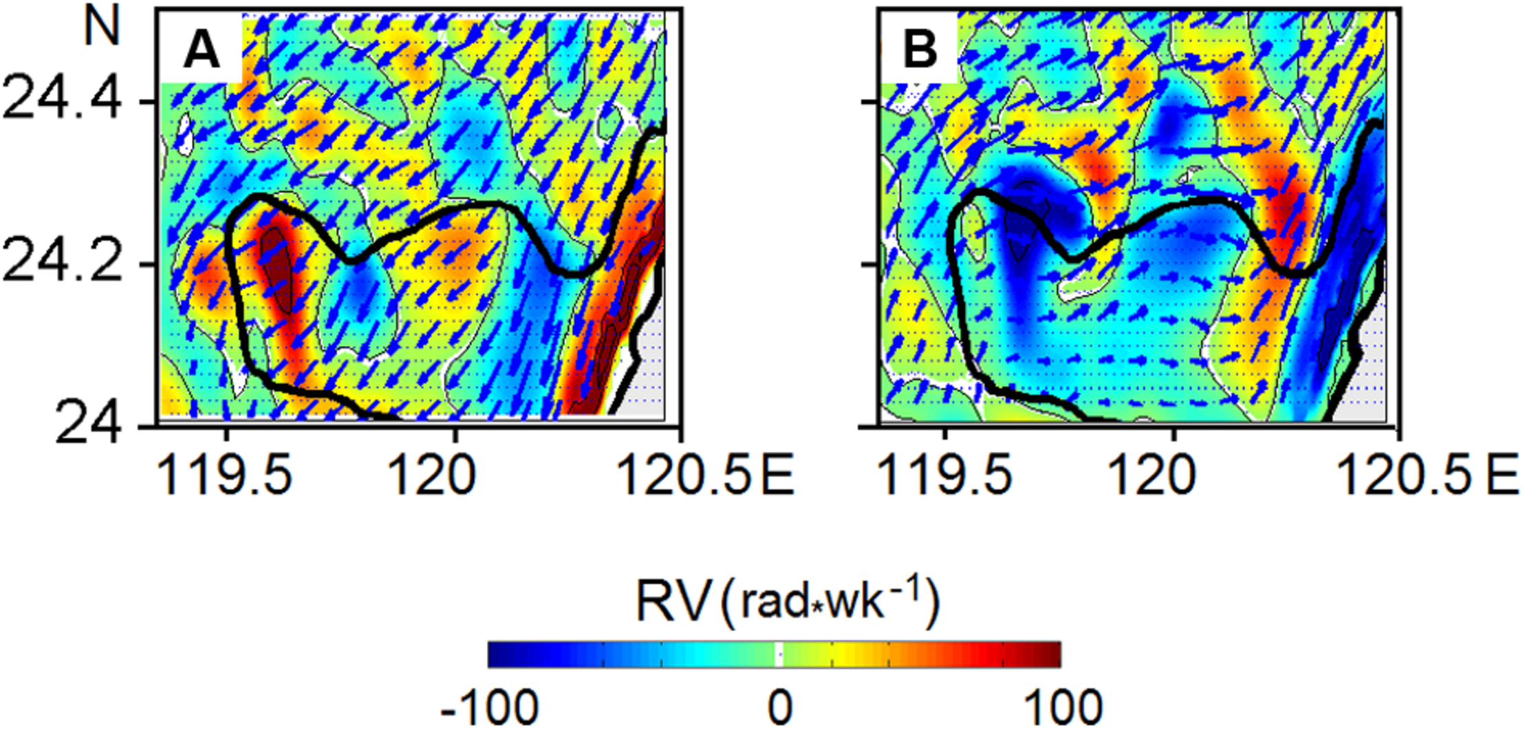
Figure 5. The successive phases of the planar distribution of relative vorticity, RV (rad/week), above the CYR at a depth of 10 m (below the surface) corresponding to peak (A) flood and (B) ebb velocities, respectively. The black line delineates the 30 m isobaths.

As can be seen in Figure 5, cyclonic eddy cores (warm shaded) over the CYR are dominant when the northward flow is developing on the flood tide (Figure 5A); anticyclonic eddy cores (cold shaded) are dominant when the northward flow is developing and impinging on the CYR on the ebb tide (Figure 5B). In both cases, the magnitudes of relative vorticity attain the rather high value of 100 rad/week (∼1.6 10^–4 rad c^–1).

Structure of Tidal Velocity in the Taiwan Strait at Different Depths

Along with the surface currents in the TS described above, in this study, we also analyzed the space-time variability of tidal currents throughout the water column, with special reference to assessing potential sites for proper deployment and operation of TECs. Such analyses are usually based on simulated depth-averaged currents, but it is often interesting to know how the TEC hub height affects the operation of TEC devices. Figure 6 presents the planar plots of instantaneous tidal current velocity at depths of 30, 50, and 60 m on peak flood and peak ebb velocities at 09:30 and 17:30 GMT, respectively, on June 27, 2013.

FIGURE 6

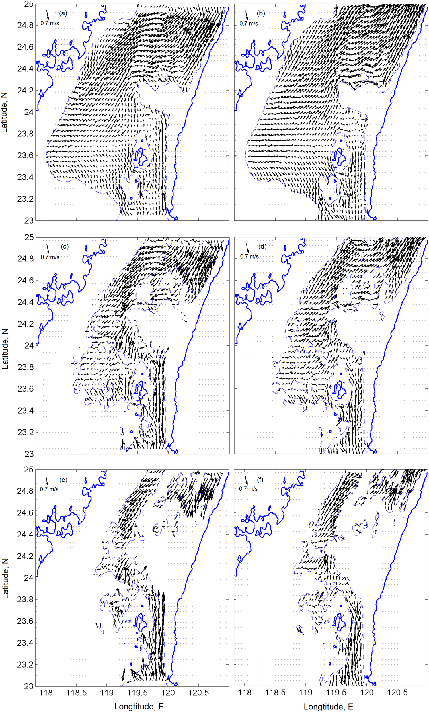
Figure 6. Tidal velocities at water depths of (a,b) 30 m, (c,d) 50 m, and (e,f) 60 m below the surface at peak velocities on the flood (at the left panel) and ebb (at the right panel). The dotted lines delineate the corresponding depths.

As shown in Figure 6, below 30 m, water from the South China Sea enters the TS through the narrow PHC on the flood and flows back to the SCS from the Strait on the ebb. As mentioned above (see Figures 3, 4), the character of the tidal current in the TS is typical for the standing wave; the flood tidal waves penetrating simultaneously into the TS from the northern and southern ends cause water in the center of the Strait to pile up and form the latitudinally directed convergence zone along 23°N. During the ebb, water coming out through both ends of the TS causes the sea level in the center of the Strait to fall and form the divergence zone along the same latitude. Generally, the tidal flow follows along the Strait, although some branches may change direction if they impinge on various obstacles on the bottom (see Figure 2) and spread along the Wuchu Depression west of the CYR. Our simulations also revealed that currents significantly intensify in the vicinity of islands and over submarine elevations and ridges, particularly along the eastern coast, where the tidal flow impinges on the CYR. Such locations would be appropriate for deploying and operating the TEC, considering the magnitude of velocity.

Note that while the lighter waters of subsurface horizons flow over the CYR (Figures 4, 6a–d), the dense bottom waters that enter from the PHC (Figures 6e,f) turn northwestward in front of the CYR. Further north, the bottom waters mixing with those lying west of the PH Archipelago enter the narrow passage (over Wuchu Depression) northwest of the CYR and move to the north as a powerful jet that reaches a maximum velocity of over 1.3 m s^–1 during the neap tide.

It should be noted that the simulations of tidal currents in the TS performed with the boundary conditions recorded during June 25–28, 2013 determined northward residual current in accordance with the observations conducted earlier by Wu and Hsin (2005), who revealed that this direction of the residual current caused a persistent negative pressure gradient along the Strait because the sea surface at the north entrance of the TS is always lower than that at the southern end. Most studies to date have indicated that the mean currents in the PHC are rather energetic and directed northward almost throughout the year (Chuang, 1985; Wu and Hsin, 2005).

Virtually the first measurement in the PHC was reported by Chuang (1985, 1986), who took current measurements near the bottom and found that tidal currents reached about 1.0 m s^–1 and the mean residual current of about 0.27 m s^–1, which was directed to the north. With the use of a ship-borne acoustic Doppler current profiler, Wang et al. (2004) later managed to map the flow field across the PHC: Their results suggested that the currents in the PHC are characterized by strong semidiurnal tides and tidal velocity exhibits multicore structure with tidal velocity exceeding 1.6 m s^–1 was detected next to the western and eastern shelf breaks of the channel. The minimum velocity was recorded over the western shoal, dropping from 1.6 to 0.8 m s^–1. The along-channel semidiurnal flow in the central deep part of the PHC was relatively uniform, with an amplitude of about 1.2 m s^–1. The phase distribution of the flow was consistent with the amplitude distribution; however, significant phase differences occurred only on the west bank, where the amplitude of the along-channel semidiurnal flow variation increased. The near-surface flow, recorded by Wang et al. (2004), lagged the near-bottom flow by about 20°, while the shallow west bank led the main channel by approximately 40°. The results of these observations are very important for seeking prospective sites for the tidal energy conversion in the PHC.

To compare the simulations with the results of the abovementioned measurements, we performed a numerical study of tidal velocity to examine the details of the structure and variability of tidal currents in the PHC. Figure 6 illustrates the simulated tidal velocity at 90 m depth covering the entire PHC. As our numerical simulations revealed, the tidal flow in the PHC is very strong and is directed meridionally because of the narrowness of the PHC. The latter is rapidly reversed from northward (Figure 7A) on the flood to southward on the ebb (Figure 7C). The structure of the tidal flow has a multicore, jet-like character; the magnitude of meridional velocity for June 25–28, 2013 was found to exceed a maximum 1.2 m s^–1 along the western slope of the PHC. The distribution of velocity at water slacks, as illustrated in Figure 7B, looks chaotic for a short period when the current decelerates and its direction turns sharply from the flood to the ebb.

FIGURE 7

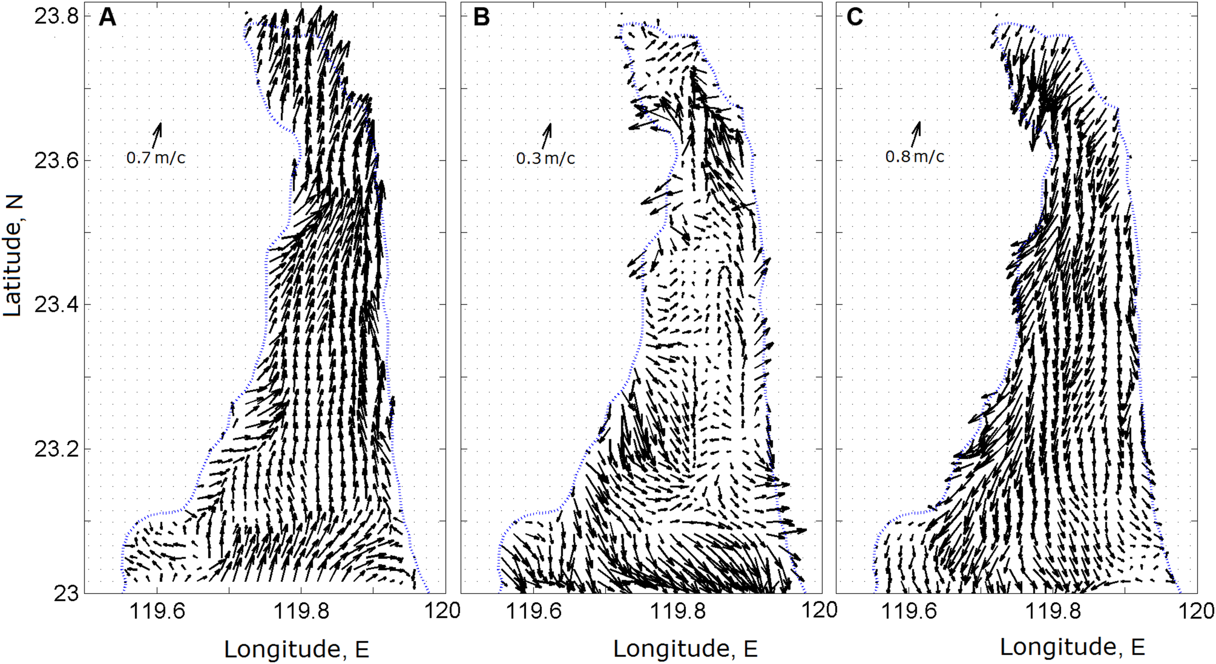
Figure 7. Tidal currents at a depth of 90 m below the surface at (A) 11:00 (at max flood elevation), (B) 14:00 (flow reversal from flood to ebb), and (C) 17:00 (at min ebb water level) on June 27, 2013.

Similar velocity variability in the PHC was observed in many other fields and numerical observations (Jan et al., 2002; Wang et al., 2004; Wu et al., 2007). The jet-like structure of the strong tidal current in the PHC, featuring only negligible asymmetry is of great interest to the developers of TEC devices. On the other hand, the turbulence of asymmetrical tidal flows should also be considered an important dynamic characteristic when assessing potential sites for power tidal energy conversion (Neil et al., 2014; McCaffrey et al., 2015; Milne et al., 2016; Korotenko and Sentchev, 2019).

Tidal Turbulence in the Peng-Hu Channel

Because the PHC has a rather deep, narrow, and flat bathymetry and its tidal currents are very strong, it is likely to be an appropriate place to deploy tidal turbines. On the other hand, due to their instability, strong currents can produce turbulence in different parts of the PHC and reduce the effectiveness of tidal turbines. To assess the possible impact of turbulence, we analyzed the distribution and time-depth variability of vertical turbulent diffusivity, K_m, in the PHC.

Figure 8 presents the distribution of K_m along the meridional section MS1 at peak velocity on the flood and ebb. The distribution of K_m on both tidal phases was very different, increasing to about 10^–2 m² s^–1 in the BBL over the CYR. Let us recall that, on the flood, a progressive tidal wave produces a southward current that enters the TS from its northern end and a northward current that enters the TS from its southern end. These opposing flows meet and create the convergence zone south of the CYR along latitude 23°N, as was mentioned above. Along roughly the same latitude, the divergence zone is created when the tidal wave produces outflowing currents at both sides of the strait on the ebb—i.e., the northward current causes an outflow of waters from the northern part of the TS while the southward current simultaneously causes an outflow of waters from the southern part of the Strait. This tidal motion, in conjunction with significant variability of density in the bottom layer of the PHC on the flood/ebb, increases or decreases stratification due to the inflow or outflow of dense or lighter bottom waters, respectively. Water inflow and outflow directions on the flood and ebb are illustrated schematically in Figure 8 by arrows. Numerical simulations show that, on the flood, strengthened stratification of dense bottom waters incoming from the SCS suppresses turbulence in the BBL (Figure 8a). This can be clearly seen in the decrease of K_m down to ∼10^–4 m² s^–1 that occurred in the BBL south of the CYR, although some patches of increased mixing (K_m ∼10^–3 m² s^–1) were predicted to occur there between 23.5°N and 23.7°N. In contrast, over the CYR and north of it, flood flow produced intense mixing (K_m ∼10^–3 m² s^–1), the latter spanning throughout the water column over the CYR (Figure 8a).

FIGURE 8

Figure 8. Vertical turbulent diffusivity, K_m, along the meridional section MS1 at peak velocity on (a) the flood and (b) on the ebb. Arrows show the direction of the flow during the flood and ebb phases.

On the ebb, the decrease of stratification due to leaving dense waters south of the CYR enhanced turbulent mixing at latitudes between 23.5°N and 23.7°N (Figure 8b). North of the CYR, zone of mixing is reminiscent of the turbulent wake produced by bottom-shear stress; furthermore, the wake is advected by the ebb flow to the north. Along the wake, one can see numerous separate patches manifesting the intensification of shear-induced turbulence (K_m ∼10^–3 m² s^–1). As seen in Figure 8b, on the ebb, the BBL over the CYR is discernibly thinner (about 10 m) than that on the flood spanning the entire layer over the CYR (Figure 8a).

The data illustrated in Figure 8 indicate that, in the PHC, turbulence near the bottom in the area between 23.7°N and 24.7°N is rather weak during both flood and ebb, so that sites within this region could be particularly suitable for mounting TECs. However, in addition to the knowledge of the turbulence intensity, it is also necessary to understand the time-depth variability of the tidal current.

Figure 9 presents the time-depth variabilities of water elevation (red line), tidal velocity (meridional component) at the surface (dash blue line) and 2 m above the bottom (dash-dot black line), as well as the logarithm of vertical turbulent diffusivity over the CYR (at Site A) and in the PCH along the meridional section 1 at Sites B–D (see Figure 1) for June 26–28, 2013.

FIGURE 9

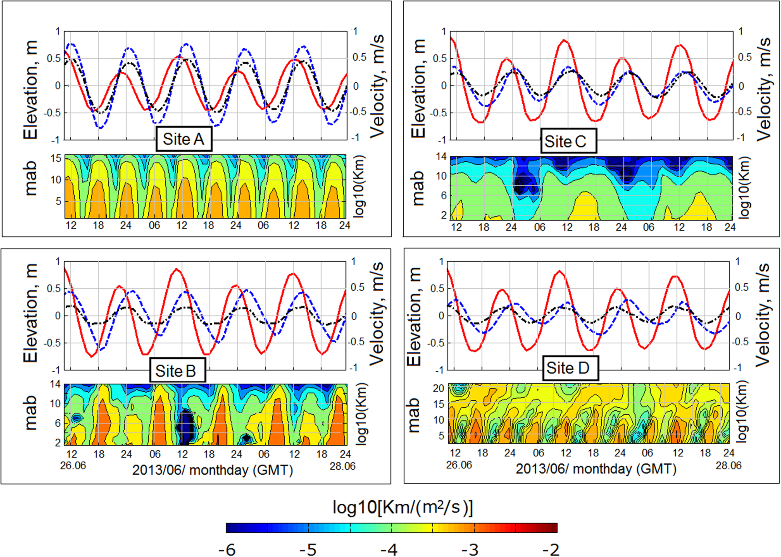
Figure 9. The time-depth variability of modeled water elevation (red line), the component of meridional velocity at the surface (dash blue line) and 2 m above the bottom (dash-dot black line), and the logarithm of vertical turbulent diffusivity K_m over the CYR (at Site A) and in the PCH along the meridional section MS1 at Sites B–D (Figure 1). Each site (A–D) consists of two panels; the upper panel illustrates water elevation and velocity and the lower panel illustrates the distribution of turbulent diffusivity throughout the water column. Abbreviation mab denotes meters above the bottom.

At Site A (Figure 9) located at the northern slope of the CYR, the velocities at the surface and bottom are synchronized and lead the changes of the water elevation. As the simulation revealed, the amplitude of velocity decreases with proximity to the bottom following the law of the wall. Eddy diffusivity K_m is related to the speed of the current and exhibits a dominant quarter-diurnal variation throughout the water column. There is some amplification of K_m during the high tide and attenuation thereof during the low tide.

Generally, the CYR area, including Site A, seems to be a proper site for the installation of TECs because of the symmetry of the flow; however, owing to intensive fishery and navigation in this region, mounting and exploiting TECs in this region might present a difficult problem. Furthermore, the high intensity of turbulence and its intermittency at Site A should be investigated with regard to their effects on the stability of TEC operation.

At the shallow southern flank of CYR (Figure 9, Site B), the meridional velocities at both the surface and the bottom change in a similar way to those at Site A during the advancing changes of the sea level, whereas the variability of K_m considerably differs from that revealed at Site A. The tidal cycle of K_m is not symmetric between the flood and ebb; the diffusivity of K_m reaches a maximum of about 5 × 10^–3 m² s^–1 at peak velocity on the ebb, regardless of the height of the tide, while on the flood K_m is significantly damped (<10^–5 m² s^–1) compared to that revealed at Site A. It should be noted that the meridional velocity becomes more asymmetrical near the bottom—i.e., as velocity decreases the ebb phase lasts longer than the flood.

At Site C, eddy diffusivity depends on variations in the tide velocity amplitude, reaching a value of about 5 × 10^–4 m² s^–1 in periods from the higher-high-water to the lower-high-water (green palette) and dropping to 10^–5 m² s^–1 from the lower-high-water to the high-low-water (cyan palette). There are bursts of turbulence during the transition of the tide from the higher-high water to the lowest-low-water (yellow palette), where K_m reaches a value of 5 × 10^–3 m² s^–1 in the 6-m BBL. According to the low level of turbulence predicted, this site could be considered promising for TECs after investigation with regard to the restrictions associated with marine traffic and fisheries.

Site D was placed at the eastern periphery of the PH Archipelago (Figure 9, Site D). Here, the eddy diffusivity K_m exhibits a dominant quarter-diurnal variation within the 20 m layer above the bottom, which distinctively consists of two turbulent layers: (1) the BBL of about 10 m, where turbulence is generated by bottom shear stress and propagates upward; combined with (2) the internal layer above the BBL in which turbulence is generated by vertical shear instability. Note that approaching the bottom, the velocity lag between neighboring layers grows noticeably, i.e., the velocity of the upper layer is greater than that of the lower layer (Figure 9, Site D). The oblique distribution of K_m over the BBL is characteristic of shear-induced turbulence, unlike turbulence generated by bottom shear stress, which is produced by sources distributed in the water column. In the BBL, maximum diffusivity K_m reaches 2 × 10^–3 m² s^–1, while in the shear-induced turbulent layer of 10 m above the BBL, maximum K_m ranges from 0.3 × 10^–3 to 0.6 × 10^–3 m² s^–1.

As our simulations indicated, the turbulence in the TS, including at the two sites considered in Figure 9 (Sites A and D), is mainly produced by bottom friction and is consistent with the quarter-diurnal variation characterizing M4 tidal oscillation (Lu and Lueck, 1999; Rippeth et al., 2002; Souza et al., 2004; Thomson et al., 2010; Korotenko et al., 2014). However, at some sites (see, for example, Sites B and C depicted in Figure 9), the quarter-diurnal turbulence cycle could be broken for a variety of reasons—for instance, the flood (or ebb) flow can considerably increase near-bottom stratification and thus limits the production of turbulence. In such a case, the variability of turbulence could follow either a quasi-semidiurnal variation, as at Site B (Figure 9), where turbulence in the BBL is suppressed by increasing density on the flood, or chaotic quasi-diurnal variations associated with meandering tidal current (see, for example, Site C depicted in Figure 9).

In some parts of the narrow, canyon-like PHC, the abrupt slopes, as well as the shear-induced mechanism, contribute to the turbulence generated by convective mixing induced by the differential transport of stratified water masses along the slope (Lorke et al., 2005). Because bottom friction and shear instability are dominant processes in the PHC, the effect of shear-induced convection is not very pronounced in the TS; nevertheless, the measurements carried out recently by Shao et al. (2018) provided solid evidence of dense water mixing by the convective mechanism. Performing and analyzing velocity measurements and turbulence dissipation obtained with a high-frequency ADCP mounted at the bottom in the northern extremity of PHC. Shao et al. (2018) discovered a rather thick near-bottom mixing layer (∼40 m), which appeared due to shear-induced convection resulting from the upwelling of the upslope flow of dense waters entering into the PHC on the flood from the south and the shear-induced turbulent mixing of the upwelled waters. The combination of these processes led to buoyancy-driven convective mixing in the BBL, which manifested as an abovementioned semi-diurnal burst of TKE dissipation rate and turbulent diffusivity on the flood.

To assess the significance of convective mixing in the PHC, Shao et al. (2018) analyzed the turbulent diffusivity of heat K_m inferred from the ADCP velocity profiles obtained. They found that in the layer of 60–100 m, K_m grew on the flood, reaching 10^–3 m² s^–1 and falling below 10^–6 m² s^–1 on the ebb (see Fig. 9 in Shao et al., 2018), revealing the fact that sources of turbulence in the PHC are of a complex and distinct nature and should be treated separately. In the case of numerical study, describing buoyancy-driven instability, in particular, requires using non-hydrostatic models.

A similar type of convective instability resulting in the development of vertical mixing in the near-bottom layer was documented by Ostrovskii and Zatsepin (2016) during measurements with an ADCP in the Black Sea. They scrutinized the convective process that unrolls the Ekman spiral near the bottom and thus drives the water in the near-bottom Ekman layer down the continental slope, resulting in the development of a thick (several tens of meters) mixed layer with neutral stratification.

Power Density Assessment

The theoretical tidal power density (P_KE) or tidal stream energy (Wm^–2) passing through a vertical cross-section perpendicular to the flow direction per unit area of this cross-section was calculated using the following formula (Carballo et al., 2009):

$$P_{KE}(t)=\frac{1}{2}\mathrm{\rho }{U}^3(t)(5)$$

where U is the magnitude of the mean horizontal tidal current. Due to Betz’s law and some potential losses in the power extraction (e.g., hydrodynamic losses, transmission losses, and generator losses), not all of this power can be converted in practice (Bahaj and Myers, 2003). These limitations related to turbine efficiency are accounted for via the power coefficient (C_P), so the effective power density (the power density that the turbine can harness) is

$$PD(t)=\frac{1}{2}{C}_p\mathrm{\rho }{U}^3(t).(6)$$

Experiments have indicated that C_P varies from 0.3 to 0.5 (Gorban et al., 2001; Ainsworth and Thake, 2006).

As it follows from Eqs (5) and (6), power density depends on velocity cubed, so even small fluctuations of velocity translate into large magnitudes of power density. The selection of hub height for a tidal turbine is thus a critical factor for asymmetrical tidal currents, as it affects the net power output. To identify prospective sites for the recommended installation of TECs in the TS, we evaluated variations of power density (PD) in the meridional (MS1–3) and zonal (ZS1–3) sections shown in Figure 1 and introduced in section “The Regionalization of the Taiwan Strait Used in This Study.” Figures 10, 11 illustrate the 20-min averaged quantities of PD for peak velocities on the flood and ebb at three zonal and three meridional sections. Tidal forcing data at both ends of the TS were used for the period of tide transition from spring to the neap tide.

FIGURE 10

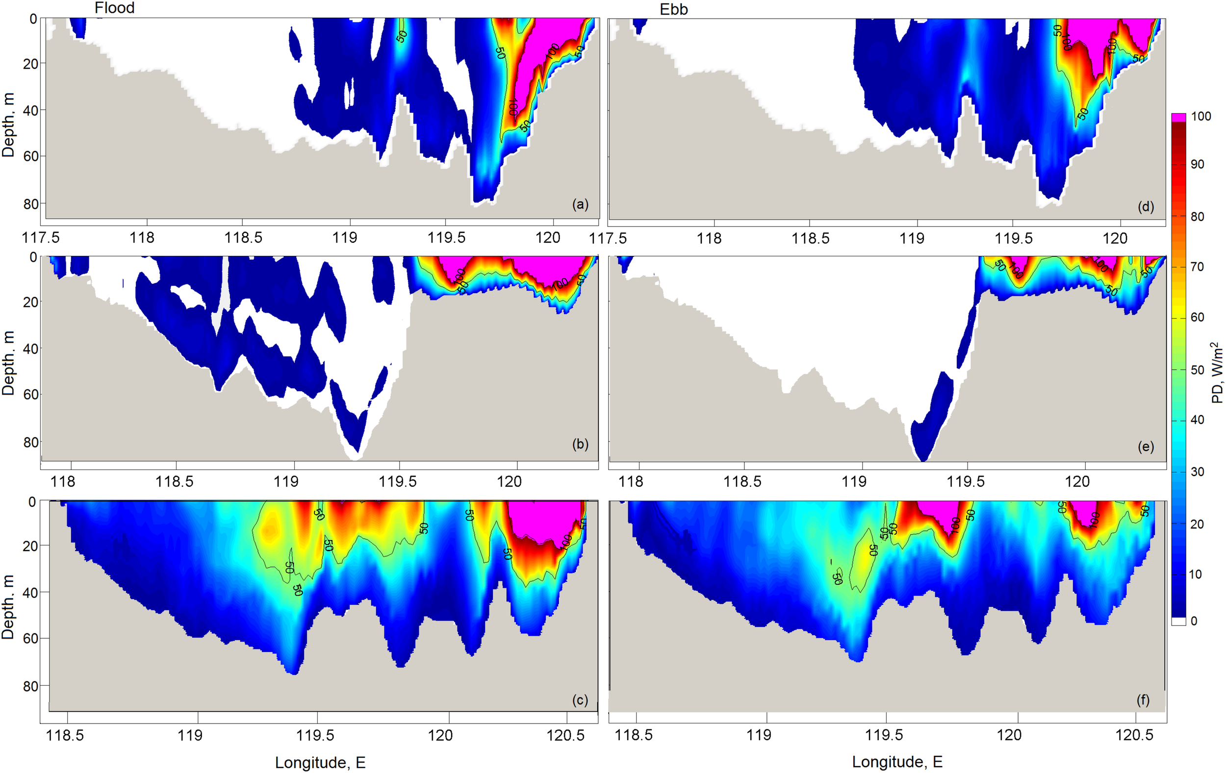
Figure 10. The 20-min averaged power density along the zonal sections for peak flood (left panel) and ebb (right panel) velocities along (a,d) ZS1, (b,e) ZS2, and (c,f) ZS3, respectively.

FIGURE 11

Figure 11. The 20-min averaged power density along the meridional sections for peak flood (left panel) and ebb (right panel) velocities along (a,d) MS1, (b,e) MS2, and (c,f) MS3, respectively.

The zonal section ZS1 is located south of the CYR and runs along latitude 23.9°N. The tidal current accelerates during both flood and ebb flow development over the eastern slope of the Strait. Magnitudes of power density on the flood and ebb are almost equal (>100 Wm^–2), indicating that the coastal tidal flow is symmetrical and thus a suitable nearshore area for mounting TECs.

The zonal section ZS2 runs along latitude 24.2°N passing over the CYR. As simulation shows, tidal energy is concentrated over the shallow plateau of the CYR and exhibits a slight asymmetry. Here, the magnitude of power density on the flood is slightly larger than that on the ebb and reaches a maximum of about 100 Wm^–2.

The zonal section ZS3 is located north of the CYR and runs along latitude 24.5°N. As the bottom topography (Figure 2) indicates, there are a number of seamounts north of the CYR that may affect the tidal current and how it is enhanced. Narrowness between such bottom features can canalize the tide and prompt the development of powerful jets, such as the multicore jet structure of tidal flow that echoes in zones of high power density over the seamounts. The maximum PD along the section varies from 80 to 100 Wm^–2. Despite the asymmetry of tidal current, the middle and eastern parts of the section ZS3 are highly likely to be appropriate for TECs installation.

The meridional section MS1 runs along longitude 119.8°E, crossing over the CYR in its central part and going through the PHC south of the CYR (Figures 11a,d). Numerical simulations indicate that most of the tidal energy along this section is concentrated over the CYR and in the PHC at approximately latitude 23.6°N east of the PH Archipelago. The power density around this location, however, exhibits significant asymmetry, so that the average peak flood magnitude is around 70% of the average peak ebb magnitude (∼300 Wm^–2), which skews power production toward the ebb stage of the tide. Nevertheless, latitude 23.6°N is a very attractive location as, in addition to the high level of available energy, there is a certain depth range (25–50 m) where the asymmetry of power density is minimal. It should be noted that Chen et al. (2013) identified the site nearby in the PHC (which we located at 23.6°N) as suitable for the installation of TECs, reporting that, in the case of the installation of turbines, the impact on water level and tidal current in the TS is expected to be minimal.

The chosen meridional section MS2 runs along longitude 119.5°N, crossing PH islands and going through the periphery of the CYR. The distribution of PD along the MS2 is determined by the characteristic enhancing of the jet-like flow along the southwestern slope of the CYR. Being trapped by the Wuchu Depression west of the CYR, both flood and ebb currents create a zone of high power density, reaching ∼100 Wm^–2. Here, large magnitudes of PD encompass almost the entire water column.

Because the abovementioned areas of convergence/divergence on the flood/ebb are located south of the CYR along the 23°N, the zone of high power density is created by the southward/northward current on the flood/ebb. The high PD zone between 24.1°N (Figure 11b) and 24.3°N on the flood looks similar to that on the ebb (Figure 11e). This location indicates a perfect symmetry of tidal current, which can be used for TEC installation.

In addition to the location considered above, we found another narrow zone of high PD centered at 24.5°N (Figure 11e) which is pronounced only on the ebb and does not appear on the flood at all (Figure 11b). This zone is associated with a narrow jet-like slope current that meanders during the tidal cycle. Such a location with an unstable current position is an example of an unsuitable site for tidal turbines. Numerical simulations also revealed a high PD zone (∼100 Wm^–2) at the end of the section MS2 (in the right-hand corners of Figures 11b,e). This location corresponds to the shallow mainland waters that are beyond our focus.

As the numerical experiment revealed, the meridional section MS3 is unsuitable as a potential TEC site. Here, the tidal currents are relatively weak, which would translate to a low power density along the entire section aside from the southern and northern ends, where tidal waves accelerate opposite currents on both phases of the tide (Figures 11c,f). The peak values of PD at both ends of this section slightly exceeded 100 Wm^–2.

Figure 12 shows the locations of prospective sites for tidal energy conversion predicted on the basis of assessing power density along the zonal ZS1–3 and meridional MS1–3 sections. The sites with a high magnitude of power density (indicated by blue stars) are located around the CYR and over seamounts in energetic jet-like tidal streams, which accelerate due to their vertical or horizontal squeezing over or between obstacles. The magnitudes of power density at those sites were found to exceed 100 Wm^–2.

FIGURE 12

Figure 12. Schematic of locations of potential sites predicted for tidal energy conversion in the Taiwan Strait. Stars denote the sites with a high power density (over 100 Wm^{– 2}) and low tide asymmetry.

The area over the CYR is certainly worthy of attention because the magnitude of power density, as was estimated, is high; however, the installation of tidal turbines at those sites may cause certain problems for navigation and fisheries. Other difficulties might be associated with oscillating turbulence. Produced by the bottom friction during the flood and ebb phases, turbulence propagates upward and may affect the entire water column in shallow areas. Note that turbulence might significantly affect the turbine power and thrust coefficients owing to the load fluctuations experienced by turbine blades, in addition to causing fatigue and unexpected failures of turbines due to unsteady blade loads (Blackmore et al., 2016; Milne et al., 2016). Therefore, taking into account the abovementioned constraints, the best sites for tidal turbine installation would be those located away from the CYR.

The most suitable potential site was found to be in the northern extremity of the PHC between the PH Archipelago and the Taiwanese coast (indicated in Figure 12 by the magenta star). As estimates indicate, the magnitude of power density here exceeds 300 Wm^–2. This site was also identified by Chen et al. (2013) as suitable for tidal energy conversion in their numerical study.

Summary and Conclusion

The present study contributes to tidal energy site resource assessments by examining the tidal currents, characteristics of turbulence, and tidal power density in the TS. For our investigation, we applied a 3-D POM adapted for the TS with tidal forcing supplied by a 2-D barotropic model. Our numerical simulations showed that the water elevation and tidal currents in the TS vary in a typical mixed semidiurnal tidal cycle and that its along-channel mean velocity amplitudes reach 1.3 m s^–1. The peculiarities of tidal circulation are determined by tidal waves that, entering the TS from the northern and southern ends, cause the center of the Strait to pile up and form zones of convergence/divergence during the flood/ebb along latitude 23°N.

Based on the POM, the high-resolution (1 nautical minute) model allowed us to evaluate the effects of bottom topography features on the enhancing of tidal currents in the TS and specifically to emphasize the enhancement of the currents over the CYR, around the PH islands, and over numerous seamounts north of the CYR where the tidal current is greatly accelerated due to a great reduction of water depth.

The high-resolution modeling also revealed that, above the CYR, the tidal current generates multicore eddy structures containing filaments of cyclonic and anticyclonic vorticity and interchange their signs when the phases of the tide change. The maximum absolute relative vorticity over the CYR was found to be about 100 rad/week.

In the cross-slope direction to the south from the CYR, turbulent asymmetry changes from ebb-dominant to flood-dominant asymmetry, and at some sites in the northern extremity of the PHC, turbulence exhibits a semi-diurnal variation as a result of the damping of turbulence by the increase of stratification on the flood due to dense water inflowing from the South China Sea. The thickness of the turbulent BBL did not exceed 15 m, with the maximum values of eddy diffusivity ranging from 10^–3 to 10^–2 m² s^–1.

Assessing the power density in the TS based on the numerical study, we identified several locations potentially appropriate for tidal energy conversion. Most of the prospective sites were identified in the vicinity and over the top of the CYR, in locations where the significant acceleration of tidal flow occurred. The tidal currents, and thus the power density at those locations, have a relatively low flood/ebb asymmetry, and the magnitude of the power density reached or exceeded 100 Wm^–2. In the PHC east of the PH Archipelago, we also identified one location that looks particularly attractive for tidal energy conversion, where power density reached 300 Wm^–2 with only an insignificant asymmetry of the tidal cycle.

Data Availability Statement

The datasets generated for this study will not be made publicly available; the results of the present numerical research are presented in figures. No datasets were used or gained.

Author Contributions

KK numerical modeling of tidal circulation, density, turbulence, and power density assessment in Taiwan Strait, comparison simulations with available data sets, and development of the overall approach and novel aspects of this study. PZ contributions to the numerical model conception and its design, acquisition and overview of hydrodynamic data and analysis of current velocity, and comparison of velocity data with up-to-date observations. Y-YC providing data on tidal circulation and water elevation in Taiwan Strait and drafting of the manuscript and critical revision of its contents. HL analysis and revision of the obtained results on the impact of turbulence on power density in the Taiwan Strait and comparison of tidal energy sites data with available observations.

Conflict of Interest

The authors declare that the research was conducted in the absence of any commercial or financial relationships that could be construed as a potential conflict of interest.

Acknowledgments

We thank the reviewers and the editor for their valuable remarks and comments. This study has been supported by the Ministry of Education and Science of Russia (Agreement 14.W03.31.0006 and themes No. 0149-2019-0003 and 0149-2019-0002) and performed in the framework of the bilateral collaboration between the National Sun Yat-sen University (NSYSU, Taiwan) and Shirshov Institute of Oceanology (SIO, Russia).

Footnotes

1. ^ Tainan Hydraulic Laboratory, Taiwan.
2. ^ https://psl.noaa.gov/dataded/data.ncep.reanalysis.derived.surface.html

References

Ainsworth, D., and Thake, J. (2006). Final Report on Preliminary Works Associated with 1MW Tidal Turbine. Emersons Green: Marine Current Turbines Ltd.

Google Scholar

Bahaj, A. S., and Myers, L. E. (2003). Fundamentals applicable to the utilization of marine current turbines for energy production. Renew. Energy 28, 2205–2211.

Google Scholar

Blackmore, T., Myers, L., and Bahaj, A. (2016). Effects of turbulence on tidal turbines: implications to performance, blade loads, and condition monitoring. Int. J. Mar. Energy 14, 1–26.

Google Scholar

Blumberg, A. F., and Mellor, G. L. (1987). A description of a three dimensional hydrodynamic model of New York harbor region. J. Hydr. Eng. 125, 799–816.

Google Scholar

Bryden, I. G., and Couch, S. J. (2006). ME1-9 marine energy extraction: tidal resource analysis. Renew. Energy 31, 133–139.

Google Scholar

Carballo, R., Iglesias, G., and Castro, A. (2009). Numerical model evaluation of tidal stream energy resources in the Ria de Muros (NW Spain). Renew. Energy 34, 1517–1524.

Google Scholar

Chapman, D. C., and Haidvogel, D. B. (1992). Formation of Taylor caps over a tall isolated seamount in a stratified ocean. Geophysical and Astrophysical Fluid Dynamics 64, 31–65. doi: 10.1080/03091929208228084

CrossRef Full Text | Google Scholar

Chen, W.-B., Liu, W.-C., and Hsu, M.-H. (2013). Modeling evaluation of tidal stream energy and the impacts of energy extraction on hydrodynamics in the Taiwan Strait. Energies 6, 2191–2203. doi: 10.3390/en6042191

CrossRef Full Text | Google Scholar

Chiou, M.-D., Chien, H., Centurioni, L. R., and Kao, C.-C. (2010). On the simulation of shallow water tides in the vicinity of the Taiwan Banks. Terr. Atmos. Ocean. Sci. 21, 45–69.

Google Scholar

Chuang, W. S. (1985). Dynamics of subtidal flow in the Taiwan Strait. J. Oceanogr. Soc. Jpn. 41, 65–72.

Google Scholar

Chuang, W. S. (1986). A note on the driving mechanisms of current in the Taiwan Strait. J. Oceanogr. Soc. Jpn. 42, 355–361.

Google Scholar

Couch, S. J., and Bryden, I. G. (2006). Tidal current energy extraction: hydrodynamic resource characteristics. Proc. Inst. Mech. Eng. Part J Eng. Marit. Environ. 220, 185–194.

Google Scholar

Cushman-Roisin, B. (1994). Introduction to Geophysical Fluid Dynamic. Upper Saddle River: Prentice Hall.

Google Scholar

Fang, G., Kwok, Y. K., Yu, K., and Zhu, Y. L. (1999). Numerical simulation of principal tidal constituents in the South China Sea, Gulf of Tonkin and Gulf of Thailand. Continental Shelf Res. 19, 845–869.

Google Scholar

Flather, R. A. (1976). A tidal model of the north-west European continental shelf. Mém. Soc. R. Sci. Liège Ser. 6, 141–164.

Google Scholar

Goddijn-Murphy, L., Woolf, D. K., and Easton, M. C. (2012). Current patterns in the inner sound (Pentland Firth) from underway ADCP data. J. Atmosph. Oceanic Technol. 30, 96–111.

Google Scholar

Gorban, A. N., Gorlov, A. M., and Silantyev, V. M. (2001). Limits of the turbine efficiency for free fluid flow. J. Energy Res. Technol. 123, 311–317.

Google Scholar

Guillou, N., Chapalain, G., and Neill, S. P. (2016). The influence of waves on the tidal kinetic energy resource at a tidal stream energy site. Appl. Energy 180, 402–415.

Google Scholar

Gunawan, B., Neary, V. S., and Colby, J. (2014). Tidal energy site resource assessment in the East River tidal strait, near Roosevelt Island, New York, New York. Renew. Energy 71, 509–517. doi: 10.1016/j.renene.2014.06.002

CrossRef Full Text | Google Scholar

Hwung, H. H., Tsai, C. L., and Wu, C. C. (1986). Studies on the correlation of tidal elevation changes along the western coastline of Taiwan. Coast. Eng. 20, 293–305.

Google Scholar

Iglesias, G., Sánchez, M., Carballo, R., and Fernández, H. (2012). The TSE index e a new tool for selecting tidal stream sites in depth-limited regions. Renew. Energy 48, 350–357.

Google Scholar

Jan, S., and Chao, S. Y. (2003). Seasonal variation of volume transport in the major inflow region of the Taiwan strait: the Penghu channel. Deep Sea Res. Part II 50, 1117–1126.

Google Scholar

Jan, S., Chern, C.-S., and Wang, J. (1994). A numerical study on currents in Taiwan Strait during summertime. La Mer 32, 225–234.

Google Scholar

Jan, S., Chern, C.-S., and Wang, J. (2002). Transition of tidal waves from the East to South China Sea over Taiwan Strait: influence of the abrupt step in the topography. J. Oceanogr 58, 837–850.

Google Scholar

Jan, S., Tseng, Y.-H., and Dietrich, D. E. (2010). Sources of water in the Taiwan Strait. J. Oceanogr. 66, 211–221.

Google Scholar

Korotenko, K., Sentchev, A., Schmitt, F. G., and Jouanneau, N. (2013). Variability of turbulent quantities in the tidal bottom boundary layer: case study in the eastern English Channel. Continent. Shelf Res. 58, 21–31. doi: 10.1016/j.csr.2013.03.001

CrossRef Full Text | Google Scholar

Korotenko, K. A., Osadchiev, A. A., Zavialov, P. O., Kao, R.-C., and Ding, C.-F. (2014). Effects of bottom topography on dynamics of river discharges in tidal regions: case study of twin plumes in Taiwan Strait. Ocean Sci. 10, 863–879. doi: 10.5194/OS-10-863-2014

CrossRef Full Text | Google Scholar

Korotenko, K. A., and Sentchev, A. V. (2019). Estimates of the turbulence intensity and power density of asymmetrical tidal flow under variable wind forcing. Izv. Atmos. Ocean. Phys. 55:196. doi: 10.1134/S0001433819020099

CrossRef Full Text | Google Scholar

Kuo, A. Y., Shen, J., and Hamrick, J. M. (1996). Effect of accceleration on bottom shear stress in tidal estuaries. J. Waterway Port Coast. Ocean Eng. 122, 75–83. doi: 10.1061/(ASCE)0733-950X1996122:2(75)

CrossRef Full Text | Google Scholar

Levitus, S. (2009). World Ocean Atlas//NOAA Atlas. Washington, DC: US Department of Commerce, NOAA/NODC.

Google Scholar

Lin, M. C., Juang, W. J., and Tsay, T. K. (2000). Applications of the mild-slope equation to compulations in the Taiwan Strail. J. Oceanogr. 56, 625–642.

Google Scholar

Liu, W. C., Hsu, M. H., and Wang, C. F. (2003). Modeling of flow resistance in mangrove swamp at mouth of tidal Keeling River, Taiwan. J. Waterway Port Coast. Ocean. Eng. 129, 86–92. doi: 10.1061/(ASCE)0733-950X2003129:2(86)

CrossRef Full Text | Google Scholar

Lorke, A., Peeters, F., and Wiiest, A. (2005). Shear-induced convective mixing in bottom boundary layers on slopes. Limnol. Oceanogr. 50, 1612–1619.

Google Scholar

Lu, Y., and Lueck, R. G. (1999). Using a broadband ADCP in a tidal channel. Part II: turbulence. J. Oceanic Atmos. Technol. 16, 1568–1579.

Google Scholar

McCaffrey, K., Fox-Kemper, B., Hamlington, P. E., and Thomson, J. (2015). Characterization of turbulence anisotropy, coherence, and intermittency at a prospective tidal energy site: observational data analysis. Renew. Energy 76, 441–453.

Google Scholar

McCann, G., Thomson, M., and Hitchcock, S. (2008). “Implications of site-specific conditions on the prediction of loading and power performance of a tidal stream device,” 2nd International Conference on Ocean Energy, Brest, France.

Google Scholar

Mellor, G. L., and Yamada, T. (1982). Development of a turbulent closure model for geophysical fluid problems. Rev.Geophys. Space Phys. 20, 851–875.

Google Scholar

Milne, I. A., Day, A. H., Sharma, R. N., and Flay, R. G. J. (2016). The characterization of the hydrodynamic loads on tidal turbines due to turbulence. Renew. Sustain. Energy Rev. 56, 851–864.

Google Scholar

Milne, I. A., SHarma, R. N., Flay, R. G. J., and Bickerton, S. (2013). Characteristics of the turbulence in the flow at a tidal stream power site. Philos. Trans. R. Soc. A 371:20120196. doi: 10.1098/rsta.2012.0196

PubMed Abstract | CrossRef Full Text | Google Scholar

Monismith, S. G., Burau, J., and Stacey, M. (1996). Stratification Dynamics and Gravitational Circulation in Northern San Francisco Bay, San Francisco Bay: The Ecosystem, ed. T. Hollibaugh, (American Association for the Advancement of Science), 123–153.

Google Scholar

Neil, S. P., Hashemi, M. R., and Lewis, M. J. (2014). The role of tidal asymmetry in characterizing the tidal energy resource of Orkney. Renew. Energy 68, 337–350.

Google Scholar

Neill, S. P., Litt, E. J., Couch, S. J., and Davies, A. G. (2009). The impact of tidal stream turbines on large-scale sediment dynamics. Renew. Energy 34, 2803–2812.

Google Scholar

Norris, J. V., and Droniou, E. (2007). “Update on EMEC activities, resource description, and characterization of wave-induced velocities in a tidal flow,” in Proceedings of the 7th European Wave and Tidal Energy Conf, Porto.

Google Scholar

Oey, L.-Y. (1996). Simulation of mesoscale variability in the Gulf of Mexico: sensitivity studies, comparison with observations, and trapped wave propagation. J. Phys. Oceanogr 28, 145–175.

Google Scholar

Ostrovskii, A. G., and Zatsepin, A. G. (2016). Intense ventilation of the Black Sea pycnocline due to vertical turbulent exchange in the Rim Current area. Deep Sea Res. I 116, 1–13.

Google Scholar

Polagye, B., and Thomson, J. (2013). Tidal energy resource characterization: methodology and field study in Admirality Inlet, Puget Sound, US, Proceedings of the Institution of Mechanical Engineers, Part A. J. Power Energy 227, 352–367.

Google Scholar

Rippeth, T. P., Williams, E., and Simpson, J. H. (2002). Reynolds stress and turbulent energy production in a tidal channel. J. Phys. Oceanogr. 32, 1242–1251.

Google Scholar

Shao, H.-J., Tseng, R.-S., Lien, R.-C., Chang, Y.-C., and Chen, J.-M. (2018). Turbulent mixing on sloping bottom of an energetic tidal channel. Continental Shelf Res. 166, 44–53. doi: 10.1016/j.csr.2018.06.012

CrossRef Full Text | Google Scholar

Sheremet, V. A. (2010). SeaHorse tilt current meter: inexpensive near-bottom current measurements based on drag principle with coastal applications. Eos Trans. 91:PO25C-13

Google Scholar

Simpson, J. H., and Hunter, J. R. (1974). Fronts in the Irish Sea. Nature 250, 404–406.

Google Scholar

Souza, A. J., Alvarez, L. G., and Dickey, T. D. (2004). Tidally induced turbulence and suspended sediment. Geophys. Res. Lett. 31:L20309. doi: 10.1029/2004GL021186

CrossRef Full Text | Google Scholar

Thomson, J., Polagye, B., Richmond, M., and Durgesh, V. (2010). Quantifying Turbulence for Tidal Power Applications. Piscataway, NJ: IEEE, 1–8.

Google Scholar

Wang, Y.-H., Chiao, L.-Y., Lwiza, K. M. M., and Wang, D.-P. (2004). Analysis of flow at the gate of Taiwan Strait. J. Geophys. Res. 109:C02025. doi: 10.1029/2003JC001937

CrossRef Full Text | Google Scholar

Wu, C.-R., Chao, S.-Y., and Hsu, C. (2007). Transient, seasonal and interannual variability of the taiwan strait current. J. Oceanogr. 63, 821–833.

Google Scholar

Wu, C.-R., and Hsin, Y.-C. (2005). Volume transport through the taiwan strait: a numerical study. TAO 16, 377–391.

Google Scholar

Yankovsky, A. E., and Chapman, D. C. (1997). A simple theory for the fate of buoyant coastal discharges. J. Phys. Oceanogr. 27, 1386–1401.

Google Scholar

Zhu, J., Hu, J.-Y., Zhang, W.-Z., Zeng, G.-N., Chen, D.-W., Chen, J.-Q., et al. (2009). Numerical Study on Tides in the Taiwan strait and its adjacent areas marine. Sci. Bull. 11, 23–36.

Google Scholar

Appendix

Model Validation

To validate the model, we have compared modeled velocity, temperature, and salinity with those obtained in special in situ measurements performed in the central part of the Taiwan Strait. For the measurements, we have deployed the current meter “SeaHorse” (Sheremet, 2010) and Standard Sea Bird’s SBE19plus instrument in coastal waters over the CYR. The measurements of velocity, temperature, and salinity were conducted at the site marked, in Figure 1, by the asterisk F. The period of data surveying (25–27 June, 2013) was characterized by the transition of the tide from the neap to the spring phase (more details in Korotenko et al., 2014).

Figure 13 illustrates current velocities obtained with the POM forced by tidal BCs versus the measurements conducted with SeaHorse current meter on 25–27 June, 2013. The instrument was deployed at the depth of 9 m, about 0.5 m above the bottom. The comparison shows a reasonably good agreement between the modeled and measured velocities, perhaps except a short distortion of the tidal cycle for unknown reasons from about 00:00 to 06:00 on June 27. The record of both measured and modeled velocities indicate the dominance of semidiurnal M2-constituent with a period of 12.42 h.

FIGURE 13

Figure 13. Series of (A) wind speed, (B) hourly averaged vectors of current velocity at the depth 9 m obtained at the mooring station (“SeaHorse”), and (C) the current velocity modeled with the POM at site F (modified from Korotenko et al., 2014).

Finally, to elucidate the effect of wind only, we have forced our model (no tide) with the constant northeasterly wind of 5 ms^–1. The modeled wind-driven current (site F) at the depth of 5m obtained thereby was below 0.05 cm s^–1, while tidal forcing produced the tidal current was as fast as up to 0.8ms^–1.