Ocean Biogeochemical Predictions—Initialization and Limits of Predictability

1. Introduction

The climate system, and the ocean physical state in particular, have been shown to be predictable several years in advance (Boer, 2004; Pohlmann et al., 2004; Smith et al., 2007; Keenlyside et al., 2008; Langehaug et al., 2017), especially at high latitudes where deep mixed layers connect the deep ocean with surface layers and the atmosphere (Boer, 2004). In the wake of these advances in near-term climate prediction, the predictability of ocean biogeochemistry is now being explored. Predictions of interannual-to-decadal variations of the ocean biogeochemical state would be useful for understanding ongoing changes in marine ecology (Séférian et al., 2014; Payne et al., 2017; Park et al., 2019), ocean pH and CO₂ uptake (Lovenduski et al., 2019), and in particular for delineating natural variations from anthropogenically forced change related to CO₂ emissions, pollution, eutrophication etc. Experiments where models' capabilities to predict reanalyses have been assessed suggest that there is potential for predicting air-sea CO₂ exchange up to several years in advance (Li et al., 2016; Séférian et al., 2018; Lovenduski et al., 2019), in particular at high latitudes where the variability of air-sea CO₂ exchange exhibits lower frequency fluctuations (Li et al., 2016; Séférian et al., 2018). Successful attempts have also been made to retro-perspectively predict observations of ocean carbon uptake and primary productivity on interannual-to-decadal time scales by only initializing physical fields (Séférian et al., 2014; Li et al., 2016, 2019; Park et al., 2019). For example, Li et al. (2016) were able to predict the observed pCO₂ in the North Atlantic Subpolar Gyre (SPG_NA) up to 3 years in advance by nudging the ocean and atmospheric models to observations. Séférian et al. (2014) found that tropical Pacific primary production could be predicted up to three years in advance when starting from physical fields nudged to the observed sea surface temperature (SST). Finally, Park et al. (2019) found a predictability of chlorophyll concentrations of up to 1 year in the tropics, and 2 years in many parts of the subtropical gyres, when starting from ocean reanalyses. In all these examples, no biogeochemical observations were used to initialize the predictions. Both Li et al. (2016) and Séférian et al. (2014) suggested that the predictability might be improved by also assimilating biogeochemical data to optimize the initial conditions, in line with e.g., Brasseur et al. (2008) and Park et al. (2018).

Due to the many difficulties associated with integrating biogeochemistry in ocean reanalyses (Park et al., 2019 and references therein), initialization of forecasts and predictions from biogeochemical observations is still under development. It has been tested on shorter time scales (days to months) and has been implemented in some operational forecast systems (Popova et al., 2002; Ciavatta et al., 2011; Fontana et al., 2013; Teruzzi et al., 2014, 2018; Gehlen et al., 2015; Simon et al., 2015; Rousseaux and Gregg, 2017; Skákala et al., 2018). On interannual-to-decadal time scales, however, the benefits that could be gained from initialized biogeochemistry have yet to be explored.

The aim of the present study is to understand whether initialization of biogeochemical state is needed for skillful biogeochemical predictions, and the mechanisms behind the predictability of ocean biogeochemistry on interannual-to-decadal time scales, with focus on export production and air-sea CO₂ exchange. To this end, we perform a suite of experiments in a perfect model framework, using the Norwegian Earth System Model (NorESM, Bentsen et al., 2013). First, we investigate the influence of errors in the biogeochemical initial state on predictions, to understand to what extent such predictions can be improved by initializing the biogeochemistry from observations. Second, we analyze differences in perfect predictability of the ocean physics vs. biogeochemistry to understand the factors that underlie, and factors that limit, the predictability of air-sea CO₂ exchange and export production.

2. Methods

2.1. Model and Simulations

The NorESM model (Bentsen et al., 2013) is a fully coupled system representing ocean dynamics (MICOM), ocean sea ice (CICE), ocean biogeochemistry (HAMOCC), atmospheric dynamics (CAM4-OSLO) including atmospheric chemistry, and land processes (CLM4) including land ice sheets and river runoff. It has been shown to reproduce the major modes of climatic variability (Bentsen et al., 2013), and has an especially good representation of ENSO variability and its teleconnections (Sperber et al., 2013; Bellenger et al., 2014; Wang et al., 2019). The ocean biogeochemical compartment in NorESM, HAMOCC, is an NPZD model with one generic class of phytoplankton, one generic class of zooplankton, dissolved and particulate organic matter, the nutrients phosphate, nitrate, silicate, dissolved iron, as well as dissolved inorganic carbon, alkalinity and oxygen. The primary production is prognostically computed as a function of phytoplankton growth rate, which is limited by incoming shortwave radiation, temperature, and availability of nutrients (phosphate, nitrate, and dissolved iron). A fixed fraction of phytoplankton and zooplankton biomass are converted into particulate organic matter, through mortality and grazing, and exported below the euphotic layer (100 m). The particulate organic matter has a constant sinking speed and remineralization rate in the ocean interior. The air-sea CO₂ fluxes are determined as the product of the air-sea CO₂ partial pressure difference, the CO₂ solubility, and the gas transfer rate, which is determined from wind speed using the parameterization by Wanninkhof (1992). The performance of the mean state of HAMOCC within NorESM was evaluated by Tjiputra et al. (2013). Perhaps more important for the present application, the variability is more difficult to evaluate due to the lack of long-term observations of ocean carbon data. But the model has been shown to perform reasonably well for ENSO-driven variability of air-sea CO₂ fluxes in the Tropical Pacific (Jin et al., 2019). The representation of the interannual variability in primary production in the Tropics has been demonstrated to be in the top three among 18 ESM's (Anav et al., 2013). Away from the Tropics, the variability of the CO₂ fluxes simulated by HAMOCC in a forced ocean configuration has been shown to compare reasonable well with observations from the Surface Ocean CO₂ Atlas in the North Atlantic (Tjiputra et al., 2012). Further, an earlier version of NorESM has been shown to be comparable to other ESM's in the representation of the effect of the North Atlantic Oscillation on carbon fluxes (Keller et al., 2012).

The present work is a first step to use HAMOCC within the framework of Norwegian Climate Prediction Model (NorCPM Counillon et al., 2014, 2016), which merges NorESM with an Ensemble Kalman Filter data-assimilation scheme, to study ocean biogeochemical predictability. The aim is to understand the benefits that could be gained from initialization of the biogeochemical state, and the mechanisms underlying biogeochemical predictability by the use of perfect model experiments. To this end, we have performed two sets of prediction experiments with ten members each, where member one is the Truth and members 2–10 are the predictions (Table 1). These experiments are initialized from a 10 member ensemble (Hist-REF), which has been integrated from 1850 to 2005 with historical forcing following the Coupled Model Intercomparison Project Phase 5 (CMIP5) protocol (Taylor et al., 2012). Each member of Hist-REF was started from different initial conditions sampled from a stable pre-industrial control run, and was run with interactive atmospheric CO₂. In our first prediction experiment, referred to as BGC_pert, we investigate the influence of perturbations in the ocean biogeochemical initial state on interannual-to-decadal predictions. The purpose is to understand the extent to which assimilation of biogeochemical observations can improve the interannual-to decadal predictability of ocean biogeochemistry. It consists of 22 10-year long simulations, starting on the first of January every fifth year between 1890 and 1995 (Figure 1). The ocean biogeochemical initial conditions for each member 1–10 in BGC_pert are taken from restarts of the corresponding member in Hist-REF, while the physical initial conditions, including also the land carbon compartment, of all members are taken from the restarts of member 1 in Hist-REF for each starting year in question. Thus, all members are starting with identical physical initial conditions of the ocean, atmosphere, land, and sea ice, while the ocean biogeochemical initial conditions differ. By using restarts from different members of the historical run for perturbing the initial conditions, we ensure that the perturbation is of the same order of magnitude as the internal (natural) variability of the model (see Figures S1, S2). Note that MICOM is an isopycnal coordinate model that uses potential density as vertical coordinates. For each isopycnal layer the mass of a biogeochemical tracer is the product of the layer thickness with the tracer concentration. In this experiment, only the concentration is perturbed while the layer thickness is the same in all members. A mismatch in the vertical grid size between the physical and biogeochemical restarts could therefore introduce an additional small perturbation in the total tracer mass. To prevent any feedback from the ocean biogeochemistry on the physical state, and to ensure that all members in BGC_pert have the same physical variability, the simulations are carried out with a prescribed atmospheric CO₂ that follows a similar evolution as the one in Hist-REF.

TABLE 1

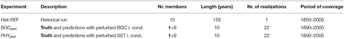
Table 1. Experimental setup.

FIGURE 1

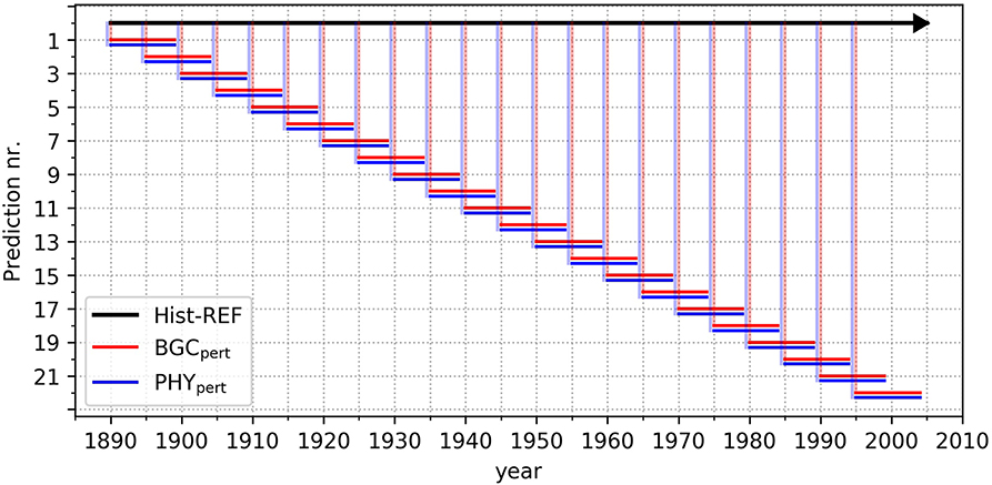
Figure 1. Experimental setup. The black, red, and blue horizontal lines show the time periods that the historical run (Hist-REF), and the prediction experiments BGC_pert and PHY_pert experiments cover. Each experiment consists of 10 ensemble members. The vertical lines illustrate that the prediction-experiments are initialized from Hist-REF. As visualized, the prediction experiments consists of 22 10-year long predictions, starting every fifth year between 1890 and 1995.

In BGC_pert we have a perfect knowledge of the initial state of the physics, leading to perfect predictions of the physical state when using a perfect model without biogeochemical feedbacks. This is never the case when doing real predictions because only a part of the ocean is observed and observations are imperfect. To investigate the extent to which the predictability of ocean biogeochemistry is limited by the predictability of physical drivers, we perform a second prediction experiment, PHY_pert. Here, both the physical and biogeochemical initial conditions for the Truth and the predictions are taken from member one in Hist-REF, but for each of the prediction members a random perturbation on the order of 10⁻¹⁰°C is added to the SST. Consequently, all members in the PHY_pert experiment have identical biogeochemical initial conditions, but physical initial conditions that are slightly different. This nanoscopic perturbation will grow rapidly with the chaotic mode of the Earth system, causing the physical state of the predictions to diverge from that of the Truth. A wide range of SST perturbations have been applied in previous perfect model experiments; from 10⁻¹⁴°C (Lovenduski et al., 2019) to 10⁻²°C (Koenigk et al., 2012). However, the system is insensitive to the exact size of the initial perturbations as they grow rapidly in the chaotic system (e.g., Lorenz, 1963, 1969). This is illustrated in Figure S3 showing the evolution of the global mean ensemble spread of SST during one of our hindcasts in the PHY_pert experiment. One month after the initialization the ensemble spread is already O(0.01°C), and after two months it is O(0.1°C). This shows that the size of the initial perturbation does not matter (as long as it smaller than the typical internal variability) for the timescales we consider in this study.

We also performed a third experiment, PHY-BGC_pert, where both the physical and biogeochemical initial conditions were perturbed. The aim of that experiment was to investigate if non-linear interactions between the physical and biogeochemical perturbations can influence the predictability. The perturbations of the biogeochemical tracers were created as in the BGC_pert experiment, while the physical conditions were perturbed indirectly by running the experiments with an interactive atmospheric CO₂. When doing so, the perturbations in the biogeochemical initial conditions translate into the atmospheric CO₂, which affects the radiation balance and consequently the SST. This way of perturbing the initial physical conditions gave similar results for the predictability as in the PHY_pert experiment, where the SST was directly perturbed (not shown). This suggests that running with an interactive CO₂ has little implication for interannual-to-decadal prediction.

2.2. Data Analysis

For the analysis we focus on the predictability of air-sea CO₂ exchange and export production, and its relations to the predictability of the ocean physics. Export production is defined as the flux of particulate organic carbon (POC) across 100 m depth. The predictive skill is quantified with anomaly correlation coefficients, (ACC, Becker et al., 2014) between the Truth and the ensemble mean of the 9 member predictions. Before the ACC was calculated, the data from the predictions were detrended in each grid cell in order to remove the main signal of the external forcing (the increase in atmospheric CO₂ due to anthropogenic emissions). This was carried out by first, in each grid cell, fitting a second-order polynomial to the time series of each variable from the ensemble mean of Hist-REF (this is illustrated for SST in Figure S4). We chose a second-order polynomial because the increase in atmospheric CO₂ concentration in the simulations follows a 2nd-order trend. Thereafter, to remove the anthropogenic signal from the 10-year long predictions and the Truth, the corresponding 10-year period of the 2nd-order trend was subtracted. After this detrending, the ACC was calculated for each lead year (τ) and grid cell (s) in the model, according to (Equation 1):

$\begin{array}{ll}ACC(s,\tau )=\frac{{\displaystyle \sum _{p=1}^P}{V}^{\prime }(s,\tau ,p)O^{\prime }(s,\tau ,p)}{\sqrt{{\displaystyle \sum _{p=1}^P}{V}^{\prime }{(s,\tau ,p)}^2{\displaystyle \sum _{p=1}^P}{O}^{\prime }{(s,\tau ,p)}^2}}& (1)\end{array}$

Where p is the prediction number and P(=22) is the total number of predictions (Figure 1), V' is the predicted value (anomaly), and O' is the truth (anomaly). We also calculated spatially averaged ACC's following (Becker et al., 2014):

$\begin{array}{ll}ACC(\tau )=\frac{\frac{{\displaystyle \sum _{p=1}^P}{\displaystyle \sum _{s=1}^S}w(s)V^{\prime }(s,\tau ,p)O^{\prime }(s,\tau ,p)}{W}}{\sqrt{\frac{{\displaystyle \sum _{p=1}^P}{\displaystyle \sum _{s=1}^S}w(s)V^{\prime }{(s,\tau ,p)}^2{\displaystyle \sum _{p=1}^P}{\displaystyle \sum _{s=1}^S}w(s)O^{\prime }{(s,\tau ,p)}^2}{W^2}}}& (2)\end{array}$

where w(s) is a local area weight (the area of the grid cell s) and W is the global sum of the area weights. When calculating the global ACC, W is the global ocean surface area.

We used a bootstrapping approach with random sampling over the starting years to compute 95% confidence intervals for the ACC's. For the spatially averaged ACCs (Equation 2) we used 1,000 bootstraps, and for the ACCs in each grid cell (Equation 1) we used 500 bootstraps due to the higher computational cost. We consider any correlation below 0.2 as no skill, i.e., having no practical value, as it only explains 4% of the variance.

The skill of the predictions is benchmarked against the skill of a persistence forecast and an uninitialized forecast. The latter quantifies the prediction skill of the remaining external forcing that is not removed with the second-order trend (e.g., volcanic forcing), and is calculated as the ACC between member one and the ensemble mean of members 2–10 in Hist-REF for the same 10-year intervals as used in the predictions (Figure 1). The persistence forecast is calculated by using the last available observation as a forecast. In our case, this is done by using output from member 1 in the historical run. For each 10-year forecast the annual mean of the year before the initialization is used as a forecast for the next 10 years; this corresponds to the autocorrelation of the quantity.

To understand the physical mechanisms behind biogeochemical predictability, we compare it to that of some key physical variables in the model. These are SST, MLD (mixed layer depth) and sea ice concentration, all of which all are important for air-sea CO₂ exchange and export (primary) production. We also compare with the predictability of sea surface height (SSH), which is a good indicator of ocean dynamics (e.g., gyre strength) and advective fluxes. Finally, we compare to the predictability of an atmospheric variable, down-welling shortwave radiation (DSW), which is important for export production and highly dependent on cloud cover. In HAMOCC the photosynthetic available radiation is assumed to be 40% of the DSW, and would therefore show the same predictability as the DSW.

For the comparison of biogeochemical vs. physical predictability, we analyse the ACC for annual and seasonal means (JFM, AMJ, JAS, OND). The seasonal means were calculated from monthly mean outputs. Unfortunately, outputs of monthly means were not saved for DSW and nutrients in Hist-REF nor in the prediction experiments, prohibiting analyses of the seasonal predictability of these variables. For the analyses we divide the ocean into three areas with different physical characteristics broadly following the biome definitions suggested by Sarmiento et al. (2004); the low latitudes oceans (LL) that are permanently stratified, 35° S to 35° N, the temperate oceans that are seasonally stratified, including temperate North Pacific (tNP: 35° N- Bering Strait), temperate North Atlantic (tNA: 35–62° N), and temperate Southern Ocean (tSO: 35–57° S), and ice covered oceans, including the Arctic Ocean (AO) and ice-covered Southern Ocean (iSO). Using this definition, there are still areas in the temperate oceans that were temporary ice-covered during the early period of study. To ensure that we do not include any effect of the sea ice on the predictability in the temperate oceans, we have masked out areas that at any year during the historical period had an annual mean ice concentration of more than 10%.

3. Results and Discussion

3.1. Impact of Perturbed BGC Initial Conditions

We start by investigating the influence of errors in the biogeochemical initial conditions on the predictability of CO₂ flux and export production. The red dots in Figure 2 show the area-weighted global mean ACC between the Truth and the predictions in the BGC_pert experiment. Lead year one is shown separately, while the longer lead times have been binned into 3-year intervals to reduce noise (this only made a difference in the PHY_pert experiment). The correlation is close to one for both export production and air sea CO₂ flux across all lead years, but somewhat lower for lead year one, showing that the evolution of the Truth and the predictions from the initial state is nearly identical. Since the predictions and the Truth were initialized with identical physical states, but different biogeochemical ones, these results show that the variability of the different members are dominated by the physics. Figure 3 shows that there is also a very strong correlation regionally, and that the effect of the perturbations in the biogeochemical initial conditions disappear after lead year one. For the air-sea CO₂ flux, the lower correlation in lead year one is mainly associated with areas of high interannual variability (Figure 3), such as the subpolar North Atlantic, the Southern Ocean and the Tropical Pacific. For export production, the areas of low correlation in the first lead year are related to the low-productive subtropical gyres, where phytoplankton growth is strongly nutrient limited due to the permanent stratification. The impact of perturbations in the biogeochemical initial conditions on the predictability of other biogeochemical quantities (e.g., nutrients and primary production) show a similar behavior (not shown).

FIGURE 2

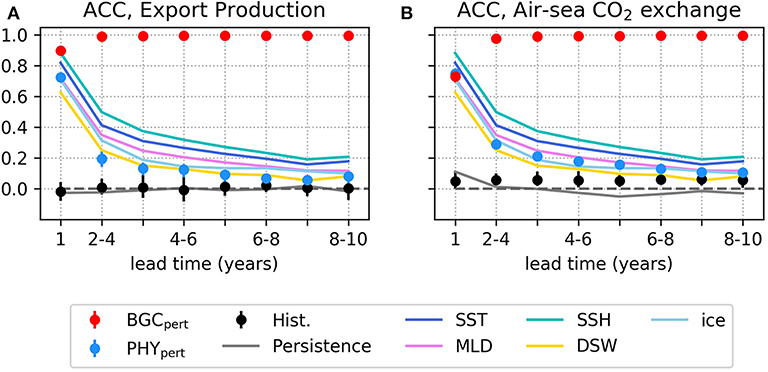
Figure 2. Globally averaged Anomaly Correlation Coefficients (ACC), for (A) export production and (B) air-sea CO₂ exchange. Black, red, and blue dots show the ACC for the export production/air-sea CO₂ exchange in the uninitialized Hist-REF run, the BGC_pert and the PHY_pert experiment, respectively, where the vertical bars show the 95% confidence intervals. The solid lines show the ACC for Sea Surface Temperature (SST), Mixed Layer Depth (MLD), Sea Surface Height (SSH), and Downwelling Shortwave Radiation (DSW) in the PHY_pert experiment. The gray solid line shows the ACC for the persistence forecast of the export production/air-sea CO₂ exchange.

FIGURE 3

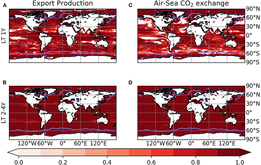
Figure 3. Anomaly correlation for the annual mean export production (A,B) and air-sea CO₂ exchange (C,D) between the Truth and the predictions, for lead years 1 and 2–4 in the BGC_pert experiment (maps for longer lead years are shown in Figures S16, S17). Only correlations that are significantly greater than (95% confidence with 500 bootstraps) the uninitialized run and persistence forecast are shown. The violet line show the maximum extent of the annual mean sea ice cover (with a minimum concentration of 10%) during the period 1890–2005.

The approach we adopted for perturbing the biogeochemistry gives perturbations that are of similar size as the natural variability of the system. This means that the perturbations are larger in areas with large interannual variability, such as the surface North Atlantic and the Southern Ocean, than in areas with lower interannual variability, such as the deep ocean and the subtropical gyres. The idea behind this strategy is to mimic the uncertainty that arise when a model is not nudged to observations, i.e., that the model state might be out of phase of the actual state of the natural system. Our results clearly show that these uncertainties in the biogeochemical initial conditions become negligible beyond the first lead year, and that the physically-driven variability dominates in the subsequent years. This suggests that a good knowledge of the physical conditions is sufficient for robust ocean biogeochemical predictions, and that assimilation of biogeochemical observations for creation of initial conditions only have the potential to add marginal skill on interannual-to-decadal predictions, at least as long as the biogeochemical fields are initialized with a reasonable climatology. It is, however, important to note that biogeochemical models are highly simplified representations of the real world, especially the ones currently used in Earth system and climate prediction models where the structure and number of tracers have to be kept relatively simple to reduce the computational cost. If increasing the complexity by for instance including more processes, interactions, functional groups and higher trophic levels that could give effects spanning over several years, or including regionally varying parameters as in Tjiputra et al. (2007) and Gharamti et al. (2017), the role of the biogeochemical initial conditions for interannual-to-decadal predictions might be of higher importance. Further, it is possible that biogeochemical models systematically underestimate biogeochemical variability (DeVries et al., 2019), meaning that the perturbations imposed here, might be lower than in the real world.

The drop in correlation in the first lead year indicates that initialization of biogeochemistry likely enhances the predictive skill on seasonal timescales.

3.2. Impact of Perturbed Physical Initial Conditions

Before investigating the physical mechanisms behind biogeochemical predictability, we will compare the predictability achieved with our experiments with the predictability presented in previously published works as an evaluation of the predictive skill in our model system.

The blue dots in Figure 2 show the global ACC between the Truth and the predictions for export production and air-sea exchange in the PHY_pert experiment, indicating the predictability when having perfect knowledge of the biogeochemical initial conditions, and starting from a slightly perturbed physical state. For export production, the correlation for lead year one is lower than that of BGC_pert suggesting that even on seasonal time scales the importance of the physical processes is larger than that of biogeochemical processes for skillfull prediction. PHY_pert show significant skill for the physics as its state is initialized with near perfect ocean and atmospheric initial condition. While the prediction skill of the atmosphere decays relatively quickly, the skill of the ocean is larger. Until lead year 2–4, the correlation exceeds the >0.2 threshold and is significantly different from the uninitialized run, indicating a predictability of a few years for both export production and air-sea CO₂ exchange. For global air-sea CO₂ exchange, the perfect predictability lies within the predictability range of 2 years presented by Lovenduski et al. (2019) and 4–6 years (computed with two different methods) by Séférian et al. (2018). The latter calculated the predictability of both the land and ocean carbon uptake, but showed that most of the long-term predictability resides in the ocean.

Figures 4, 5 show ACC maps of the annual mean export production and air-sea CO₂ exchange between the Truth and the mean of the predictions in the PHY_pert experiment. Similar maps for seasonal means and other biogeochemical fields, are shown in Figures S18–S26. In lead year one there is a strong (> 0.5) correlation, indicating predictability almost everywhere in the global ocean for the air-sea CO₂ exchange. Exceptions are the poleward halves of the subtropical gyres and the ice-covered Arctic Ocean. The pattern looks similar for the export production, with the exception of a low predictability in the Northern Hemisphere subpolar oceans. As the predictions are initialized on the first of January, the better predictability of the Southern Hemisphere export production in lead year one is expected. The reason for why there is essentially no predictability of export production at northern latitudes in lead year 1 will be explored in section 3.3.

FIGURE 4

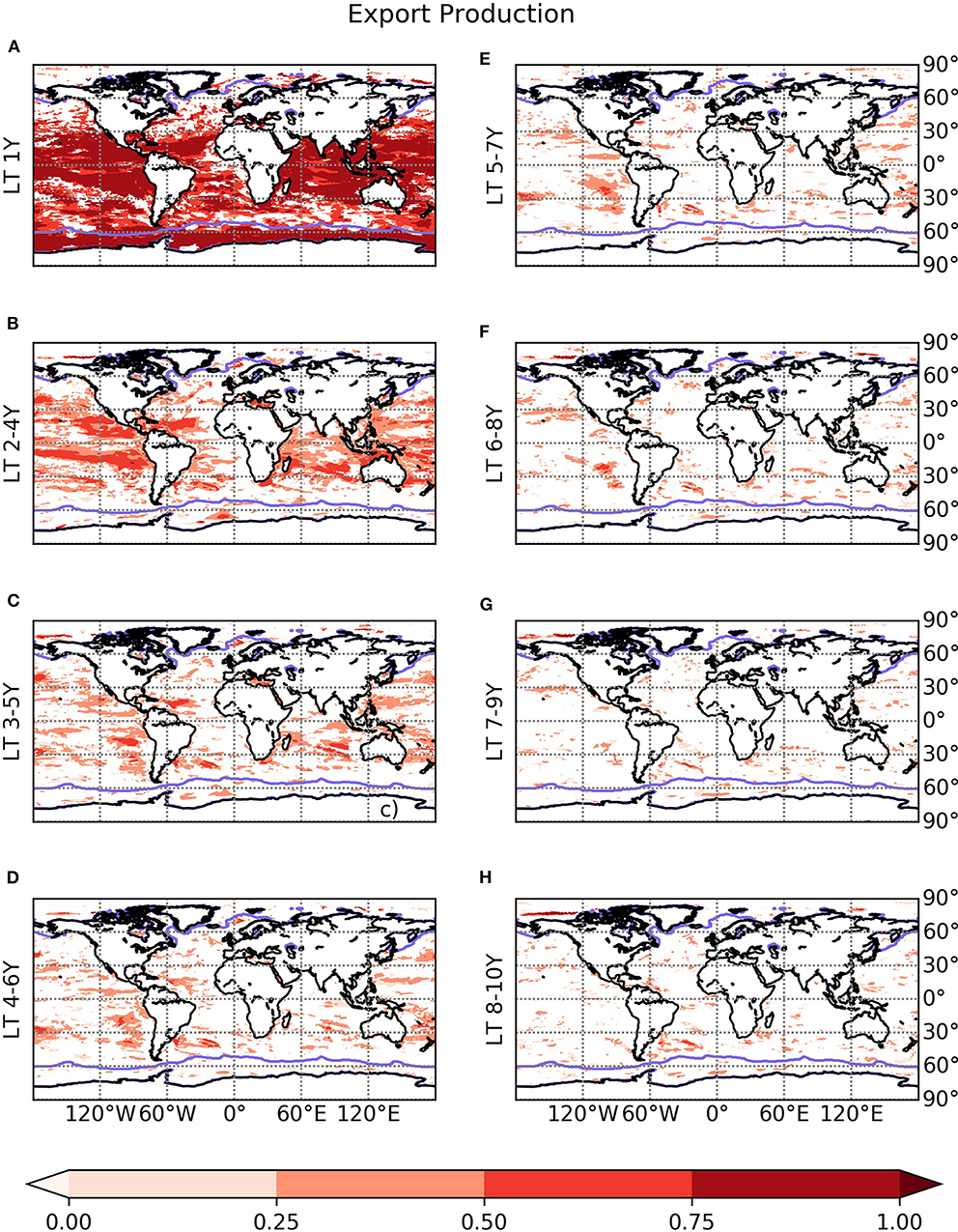
Figure 4. Anomaly correlation for the annual export production between the Truth and the predictions, for different lead years (A–H) in the PHY_pert experiment. Only correlations that are significantly greater than (95% confidence with 500 bootstraps) the uninitialized run and persistence forecast are shown. The violet line show the maximum extent of the annual mean sea ice cover (with a minimum concentration of 10%) during the period 1890–2005.

FIGURE 5

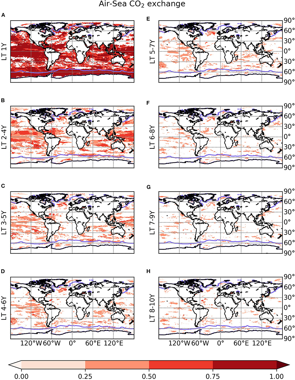
Figure 5. Anomaly correlation for the annual mean air-sea exchange between the Truth and the predictions, for different lead years (A–H) in the PHY_pert experiment. Only correlations that are significantly greater than (95% confidence with 500 bootstraps) the uninitialized run and persistence forecast are shown. The violet line show the maximum extent of the annual mean sea ice cover (with a minimum concentration of 10%) during the period 1890–2005.

For longer lead times, the predictability of the CO₂ exchange quickly degrades, except for in a few areas. In the tropical and subtropical oceans, in particular in the Pacific, there is predictability until lead years 2–4 for air-sea CO₂ exchange. The longest predictability is observed in the SPG_NA, where there is a relatively strong correlation until lead year 5–7. This agrees well with Li et al. (2016), who found potential predictability of the winter CO₂ exchange of up to 4–7 years in the western SPG_NA. Apart from the SPG_NA, the predictability of air-sea CO₂ exchange quickly degrades in the high latitude oceans, including the Southern Ocean. Here, a coherent pattern of predictability can only be seen until lead year 2–4. The spatially averaged ACC over the Southern Ocean indicates a predictability of 1 year (Table 2). This short predictability agrees fairly well with Lovenduski et al. (2019) who found a significant predictability of up to two years in the Southern Ocean, but is lower than Séférian et al. (2018) who found a predictability of 4–6 years. The difference in predictability found here and by Lovenduski et al. (2019) compared to Séférian et al. (2018) could be related to the differences in the model and simulation setup. It should be noted that while Séférian et al. (2018) made their predictions under pre-industrial forcing, the predictions in the current study and in Lovenduski et al. (2019) were carried out using historical forcing. It is possible that the biogeochemistry becomes less predictable under present forcing. Another reason could be differences in the implementation and parameterization of primary production, which has been shown to be important for regulating the air-sea CO₂ fluxes in the Southern Ocean (Kessler and Tjiputra, 2016). This will be further discussed in the following sections.

TABLE 2

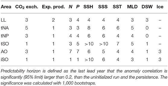
Table 2. Predictability horizon in years for annual mean air-sea CO₂ exchange, export production, nitrate, phosphate, sea surface height, sea surface salinity, sea surface temperature, mixed layer depth, downwelling shortwave radiation and sea ice concentration in Low latitudes (LL), temperate North Atlantic (tNA), temperate North Pacific (tNP), temperate Southern Ocean (tSO), Arctic Ocean (AO), and ice-covered Southern Ocean (iSO).

For export production (Figure 4), the predictability stays significant in the low latitudes until lead year 2–4, in agreement with Séférian et al. (2014), who found a predictability of NPP (Net Primary Production) of up to 3 years in the tropical Pacific. Due to their strong linkage, the predictability of primary production and phytoplankton concentration is similar to that of export production in our model (Figures S22, S23). As with the air-sea CO₂ exchange, the predictability of the export production quickly degrades in high latitudes in PHY_pert, but in contrast, almost no predictability is evident in the SPG_NA.

The good agreement of the predictability achieved in our perfect model experiment with perturbed SST with the predictability found in other studies with different models, suggest that our model system has a reasonable representation of the mechanisms giving rise to predictability.

The relatively short predictability of air-sea CO₂ exchange (except in the SPG_NA) and especially export production in the high latitudes, as shown in Figures 4, 5, is rather unexpected. Due to the strong control that ocean physics exerts on ocean biogeochemistry, it has been hypothesized that the long predictability that has been shown to reside in the ocean, in particular for SST and sea surface salinity (SSS) in the Southern Ocean and the North Atlantic (Pohlmann et al., 2004; Zhang et al., 2017; Buckley et al., 2019 and Figures S27–S29, S33), should result in a long predictability for ocean biogeochemistry (e.g., Li et al., 2016; Séférian et al., 2018; Lovenduski et al., 2019). The reason for this lack of predictability will be explored in section 3.3.

3.3. Sources and Limits of Predictability

To understand the physical factors that give rise to or limit the predictability of export production and air-sea CO₂ exchange, we will compare it to the predictability of various physical variables. The idea behind this is that the least predictable physical variable (among those known for having a considerable direct, or indirect, impact on biogeochemical variability) should set the predictability horizon of the ocean biogeochemistry. In Figures 2, 6–8 we have therefore plotted the regionally averaged ACC for SSH, SST, MLD, sea ice, and DSW, together with the ACC for air-sea CO₂ exchange, for annual and seasonal means. The predictability of export production aligns closely with that of the summer air-sea CO₂ exchange and is therefore shown in the supplementary material (Figures S7–S9). Correlation maps showing the skill for physical properties are shown in Figures S27–S39.

FIGURE 6

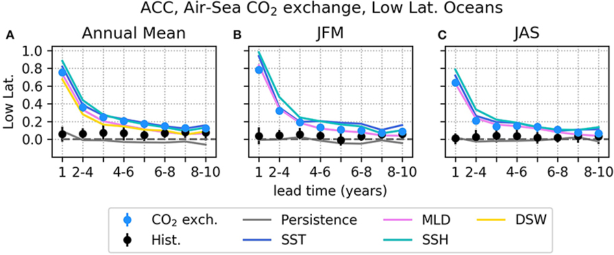
Figure 6. Spatially averaged Anomaly Correlation Coefficients (ACC) for low latitude oceans, for (A) annual means, (B) January–March means, and (C) July-September means. Black and blue dots show the ACC for the air-sea CO₂ exchange in the uninitialized run (Hist-REF) and the PHY_pert run, respectively, where the vertical bars show the 95% confidence intervals. The solid lines show the ACC for Sea Surface Temperature (SST), Mixed Layer Depth (MLD), Sea Surface Height (SSH), and Downwelling Shortwave Radiation (DSW) in the PHY_pert experiment. The gray solid line shows the ACC for the persistence forecast of air-sea CO₂ exchange.

For the global annual means (Figure 2), we note that SSH has the overall highest predictability, followed by SST, MLD and sea ice, while DSW has the lowest. This is expected since the atmosphere has a shorter memory than the ocean (Koenigk et al., 2012; Roberts et al., 2016) and the DSW is influenced by the cloud cover, which is highly unpredictable. Variations in SSH are, on interannual timescales, a measure of dynamically induced density and ocean circulation changes. In regions that are less stratified SSH represents a column-integrated signal, while in regions where the 1.5 layer approximation holds (i.e., an active less dense layer over a much thicker and denser inactive layer) SSH variations closely relate to upper ocean (density) changes (Wyrtki and Kendall, 1967; Rebert et al., 1985). This relation is strongest in the tropics where the density contrast between the two layers is the greatest. SST and MLD by definition represent surface processes, which away from the tropics are more sensitive to the atmospheric variability than SSH, and therefore are less predictable. The MLD is in general less predictable than the SST (also seen in Figures S27, S30), with the largest difference in the Southern Ocean.

3.3.1. Low Latitude Oceans

In the low latitude oceans (Figure 6), the predictability is similar across the physical variables, and there is an overall perfect-model predictability of 3–5 years, even for DSW (Table 2). This is a result of the strong coupling between ocean and atmospheric variability through atmospheric convection in this region that influences the cloud cover and consequently the DSW (Yan, 2005; Sun et al., 2017). The predictability of air-sea CO₂ exchange and export production is similar to that of the physical properties. Because of the small seasonal variations, the predictability of the annual and seasonal means are similar (Figure 6 and Tables 2–4).

Séférian et al. (2014) suggested that the predictability of primary production in the low latitude Pacific is tied to the poleward advection of nutrients anomalies that are initially induced by the ENSO-driven variations in upwelling of nutrients at the Equator. Another, slightly different explanation of the predictability in this region is found in Polkova et al. (2015) and Roberts et al. (2016). They suggested that the predictability of the SSH (up to 2–5 years lead time) in the subtropics is a result of baroclinic Rossby-waves, carrying the signal of the initial conditions westward. This would also apply to ocean biogeochemistry, as Rossby waves modify horizontal velocities and the vertical displacement of the thermocline, which affects the horizontal advection and exchange of nutrients and carbon with deep waters (e.g., Uz et al., 2001; Sakamoto et al., 2004; Charria et al., 2008). Indeed, the spatial pattern of predictability in the low latitude Pacific shown in Figures 4, 5 resembles the spatial pattern of the Rossby-wave front presented in Figure 4 of Chelton and Schlax (1996). The links between the predictability and ENSO as suggested by Séférian et al. (2014), and to off-equatorial baroclinic Rossby-waves as suggested by Polkova et al. (2015) and Roberts et al. (2016), are however not incompatible, as these waves have been shown to be triggered by ENSO events (Battisti, 1989; Kessler, 1991).

3.3.2. Temperate Oceans

In the temperate oceans there is a large spread in the predictability of the various physical variables (Figure 7 and Table 2), in contrast to what was shown for the low latitudes in the previous section. It ranges from 0 to 1 year for the annual mean DSW, via 4–7 years for the SST and MLD, and up to 6- >10 years for the SSH. The variability of DSW in these regions is influenced by the synoptic scale variability and mid-latitude depressions, which are highly unpredictable beyond timescales of a few days. The higher predictability of SSH, SST, and MLD than in the low latitudes is related to the stronger coupling between the surface and deep oceans through winter convection and mixing (e.g., Boer, 2004). The predictability of the annual mean CO₂ exchange is 1 and 3 years in the tSO and tNP, respectively, and 5 years in the tNA. Due the strong seasonality of air-sea CO₂ exchange, an analysis of its seasonal predictability is needed to understand the underlying physical mechanisms.

FIGURE 7

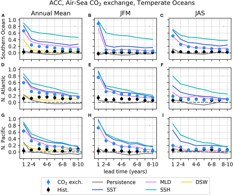
Figure 7. Spatially averaged Anomaly Correlation Coefficients (ACC) for temperate oceans including Southern Ocean (A–C), North Atlantic (D–F) and North Pacific (G–I), for annual means (left column), January-March means (middle column), and July-September means (right column). Black and blue dots show the ACC for the air-sea CO₂ exchange in the uninitialized run (Hist-REF) and the PHY_pert run, respectively, where the vertical bars show the 95% confidence intervals. The solid lines show the ACC for Sea Surface Temperature (SST), Mixed Layer Depth (MLD), Sea Surface Height (SSH), and Downwelling Shortwave Radiation (DSW) in the PHY_pert experiment. The gray solid line shows the ACC for the persistence forecast of air-sea CO₂ exchange.

From the seasonal decomposition (Figure 7 and Tables 3, 4, decomposition into OND and AMJ means are shown in Figures S10-S15), it is clear that the predictability of the summer CO₂ exchange is poor, and that the predictability of the annual mean CO₂ exchange originates from a predictable winter state. The ACC of the winter CO₂ exchange is similar to the ACC of the winter MLD (both in amplitude and in duration), which suggests that the predictable signal originates from the winter vertical mixing and the upwelling of DIC-rich deep waters to the surface. This is consistent with Fröb et al. (2019), who observed a strong relation between interannual variations in DIC, pCO₂, and MLD in in situ measurements from the subpolar North Atlantic.

TABLE 3

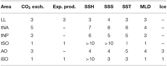
Table 3. Same as Table 2 but for January–March means.

TABLE 4

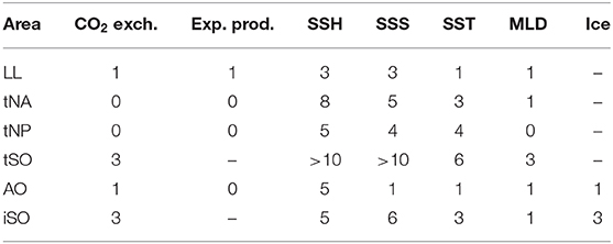
Table 4. Same as Table 2 but for July–September means.

It is interesting to note that the predictability of MLD in the North Atlantic is aligned with the predictability of SST, while this relationship is much weaker in the North Pacific and in the Southern Ocean. The depth of the mixed layer is dependent on both mechanical (wind) forcing and buoyancy forcing. In parts of the ocean where there is a large heat release to the atmosphere, the oceanic memory in form of heat content has a relatively larger impact on the mixed layer than the atmospheric forcing. This could explain the better predictability of MLD, and consequently the CO₂ exchange, in the tNA in comparison to the tSO and tNP, as the heat loss to the atmosphere is larger in the North Atlantic (e.g., Talley et al., 2011 and Figure S5).

From Figure 7 it becomes clear that the low predictability of the summer CO₂ exchange (and export production) can be related to an overall low predictability of the ocean physical state; which comes as a result of the stronger control that the unpredictable atmosphere exerts on the upper ocean during this season when the mixed layer depth is shallow and the exchanges between upper and deep ocean water masses are limited. Interestingly, the predictability of the annual mean nutrient concentrations is better than that of export production (Table 2), suggesting that predictability of annual mean nutrient concentrations does not necessarily lead to predictability of annual mean export production in temperate oceans, i.e., the unpredictable dynamics of the summer mixed layer (including light availability and exchange of nutrients with the deep waters) is more important.

3.3.3. Ice-Covered Oceans

As one of the regulators of gas exchange and the amount of light and momentum reaching the upper ocean, sea ice has a considerable impact on air-sea CO₂ exchange and export production. There is also an indirect control of the sea ice on these processes as its melting and formation influences the buoyancy and thus the mixed layer depth. The predictability of sea ice should therefore have an impact on the predictability of CO₂ exchange and export production.

Figure 8 and Table 2 show that there is a mean predictability of sea-ice concentration of 3 years in the Arctic Ocean and in the Southern Ocean, which is in agreement with other studies for the annual mean ice cover (Guemas et al., 2016) and with a conceptual model for the Barents Sea (Onarheim et al., 2015). As expectedly shown in Figure 8, the predictability of the annual mean CO₂ exchange agrees well with that of the sea ice in the Arctic Ocean. This is however not the case in the Southern Ocean, where the CO₂ is only predictable on a time horizon of one year compared to three years for sea ice.

FIGURE 8

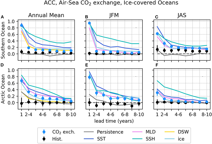
Figure 8. Spatially averaged Anomaly Correlation Coefficients (ACC) for ice-covered oceans including Southern Ocean (A–C), and Arctic Ocean (D–F), for annual means (left column), January-March means (middle column), and July-September means (right column). Black and blue dots show the ACC for the air-sea CO₂ exchange in the uninitialized run (Hist-REF) and the PHY_pert run, respectively, where the vertical bars show the 95% confidence intervals. The solid lines show the ACC for Sea Surface Temperature (SST), Mixed Layer Depth (MLD), Sea Surface Height (SSH), and Downwelling Shortwave Radiation (DSW) in the PHY_pert experiment. The gray solid line shows the ACC for the persistence forecast of air-sea CO₂ exchange.

From the seasonal decomposition of the predictability in iSO and AO, we note that the predictable signal of the CO₂ exchange also in these regions comes from the winter state, and that it closely follows the predictability of sea ice concentration and MLD (Figure 8 and Tables 3, 4). As for the temperate oceans, the predictability of the summer CO₂ exchange, MLD and sea ice concentration is practically absent, indicating a large influence of the atmospheric forcing during this season.

The relative importance of the seasons for the annual mean predictability depends on how much the interannual variations of the summer and winter means contribute to the interannual variations in annual means, and how predictable they are. For example, in regions where the interannual variability in CO₂ exchange during summer dominates over that in winter, the predictability of the annual mean CO₂ exchange will be lower than that of the winter. If, however, the winter variability contributes to a large part of the interannual variability (as would be the case for MLD), the predictability of the annual mean will approach that of the winter state. This could explain the differences in predictability of air-sea CO₂ exchange in the Southern Ocean between the present study and Séférian et al. (2018). It could also explain why the predictability of the annual mean CO₂ exchange is lower than the predictability of the annual mean sea ice cover in iSO, even though they compare well in summer and winter, i.e., interannual sea ice variability is driven by winter variations, while that of CO₂ exchange is driven by summer variations.

4. Conclusions

In this study we have performed two perfect model experiments with the aim to investigate (i) to what extent perturbations in the initial state of biogeochemical tracers influence inter-annual to decadal predictions of ocean biogeochemistry and (ii) to understand the physical mechanisms that gives rise to, or limit, predictability of biogeochemical processes such as air-sea CO₂ exchange and export production.

Perturbations in biogeochemical initial conditions only degrade predictions in the first lead year. In the following lead years the ocean biogeochemistry re-adjusts to the physics, and the influence of perturbations in the initial conditions becomes negligible. This suggests that initialization of biogeochemistry through e.g., assimilation of biogeochemical observations only brings marginal improvements to interannual-to-decadal biogeochemical predictions, while the initialization of the physics is of high importance, at least in climate prediction models with a similar complexity as the one used in the current study. The results may change if a more complex biogeochemical model, e.g., one that includes higher trophic levels, is used. To further assess the robustness of our findings, similar experiments should be conducted with other models, in particular those with enhanced complexity. Further, assimilation of biogeochemical observations would be useful for example for parameter estimation, and could be used to improve the initial physical fields (Yu et al., 2018), especially in remote parts of the oceans that are poorly sampled. Despite our results, it is therefore still important to develop this technique.

The predictability horizon that we achieve in our perfect model experiment with perturbed SST agrees overall with other studies using different models, suggesting that our model setup has a reasonable representation of the mechanisms giving rise to predictability. For export production, we found the longest predictability in low latitude oceans, with a similar time scale of predictability as baroclinic Rossby waves (Polkova et al., 2015). In seasonally stratified oceans, there is almost no predictability of export production, even in areas that show strong predictability of annual mean ocean physics and nutrients. This is related to the low predictability of the summer mixed layer that is under strong influence by the unpredictable atmosphere. As a result, the summer air-sea CO₂ exchange, which is predominantly driven by biological productivity in temperate seasonally stratified oceans (Tjiputra and Winguth, 2008; Tjiputra et al., 2014), also shows weak predictability. The predictability of the winter air-sea CO₂ exchange shows a strong relation to the winter mixed layer depth in temperate oceans. In the Southern Ocean and the North Pacific the predictability of the winter mixed layer is weaker than that of the sea surface temperature, which we suggest to be because of its higher sensitivity to the wind (Figure S6). The relatively long predictability of air-sea CO₂ exchange (and mixed layer depth) in the temperate North Atlantic is explained by the strong impact the ocean thermal memory has on the heat release and on the buoyancy forcing in this area.

To conclude, our results call into question the utility of biogeochemical observations for initialization of biogeochemical predictions. It is however important to note that this is based on results from perfect model experiments with one model system only. Similar experiments should be performed using models with more complex, and potentially more correct representation of marine biology and biogeochemistry. Further, we have shown that the predictability of the mixed layer depth is overall less than that of ocean temperature and salinity and therefore puts an important constraint on the predictability of export production and air-sea CO₂ fluxes. A more throughout investigation of the predictability of the mixed layer depths (in particular during summer) in the real world, which is not very well-explored, is therefore needed to better understand real world biogeochemical predictability.

Data Availability Statement

The datasets generated for this study will be made available at the NorStore research data archive upon publication (https://archive.sigma2.no/).

Author Contributions

The numerical simulations were run by FF and JT, with inputs and suggestions from FC, IB, AS, AN, and AO. All authors were active in discussing and interpreting the results. FF lead the writing of the manuscript with inputs from all co-authors.

Funding

FF was funded by the Nansen Legacy project (276730). JT acknowledges project RCN-COLUMBIA (275268) and H2020-TRIATLAS (817578). FC received funding from the Trond Mohn Foundation, under project number : BFS2018TMT01 and the Norwegian Research Council projects INES (270061). IB was funded by the Trond Mohn Foundation, BFS2018TMT01. AS acknowledges project H2020-TRIATLAS (817578).

Conflict of Interest

The authors declare that the research was conducted in the absence of any commercial or financial relationships that could be construed as a potential conflict of interest.

Acknowledgments

We acknowledge UNINETT Sigma2 (the national infrastructure for computational science in Norway, projects NS1002K and NN1002K, NN9039K and NS9039K) for providing the resources for performing the simulations and analysing/storing the output at the Fram, Vilje and Nird systems. We want to thank the two reviewers for their constructive comments.

Supplementary Material

The Supplementary Material for this article can be found online at: https://www.frontiersin.org/articles/10.3389/fmars.2020.00386/full#supplementary-material

References

Anav, A., Friedlingstein, P., Kidston, M., Bopp, L., Ciais, P., Cox, P., et al. (2013). Evaluating the land and ocean components of the global carbon cycle in the CMIP5 earth system models. J. Clim. 26, 6801–6843. doi: 10.1175/JCLI-D-12-00417.1

CrossRef Full Text | Google Scholar

Battisti, D. S. (1989). On the role of off-equatorial oceanic rossby waves during ENSO. J. Phys. Oceanogr. 19, 551–560. doi: 10.1175/1520-0485(1989)019<0551:OTROOE>2.0.CO;2

CrossRef Full Text | Google Scholar

Becker, E., den Dool, H. v., and Zhang, Q. (2014). Predictability and forecast skill in NMME. J. Clim. 27, 5891–5906. doi: 10.1175/JCLI-D-13-00597.1

CrossRef Full Text | Google Scholar

Bellenger, H., Guilyardi, E., Leloup, J., Lengaigne, M., and Vialard, J. (2014). ENSO representation in climate models: from CMIP3 to CMIP5. Clim. Dyn. 42, 1999–2018. doi: 10.1007/s00382-013-1783-z

CrossRef Full Text | Google Scholar

Bentsen, M., Bethke, I., Debernard, J. B., Iversen, T., Kirkevåg, A., Seland, Ø., et al. (2013). The Norwegian Earth System Model, NorESM1-M-Part 1: description and basic evaluation of the physical climate. Geosci. Model Dev. 6, 687–720. doi: 10.5194/gmd-6-687-2013

CrossRef Full Text | Google Scholar

Boer, G. J. (2004). Long time-scale potential predictability in an ensemble of coupled climate models. Clim. Dyn. 23, 29–44. doi: 10.1007/s00382-004-0419-8

CrossRef Full Text | Google Scholar

Brasseur, P., Gruber, N., Barciela, R., Brander, K., Hobday, K., Huret, M., et al. (2008). Integrating biogeochemistry and ecology into ocean data assimilation systems. Oceanography 22, 206–215. doi: 10.5670/oceanog.2009.80

CrossRef Full Text | Google Scholar

Buckley, M. W., DelSole, T., Lozier, M. S., and Li, L. (2019). Predictability of North Atlantic Sea surface temperature and upper-ocean heat content. J. Clim. 32, 3005–3023. doi: 10.1175/JCLI-D-18-0509.1

CrossRef Full Text | Google Scholar

Charria, G., Dadou, I., Cipollini, P., Drévillon, M., and Garçon, V. (2008). Influence of Rossby waves on primary production from a coupled physical-biogeochemical model in the North Atlantic Ocean. Ocean Sci. 4, 199–213. doi: 10.5194/os-4-199-2008

CrossRef Full Text | Google Scholar

Chelton, D. B., and Schlax, M. G. (1996). Global observations of oceanic rossby waves. Science 272, 234–238. doi: 10.1126/science.272.5259.234

CrossRef Full Text | Google Scholar

Ciavatta, S., Torres, R., Saux-Picart, S., and Allen, J. I. (2011). Can ocean color assimilation improve biogeochemical hindcasts in shelf seas? J. Geophys. Res. 116:C12043. doi: 10.1029/2011JC007219

CrossRef Full Text | Google Scholar

Counillon, F., Bethke, I., Keenlyside, N., Bentsen, M., Bertino, L., and Zheng, F. (2014). Seasonal-to-decadal predictions with the ensemble Kalman filter and the Norwegian Earth System Model: a twin experiment. Tellus A 66:21074. doi: 10.3402/tellusa.v66.21074

CrossRef Full Text | Google Scholar

Counillon, F., Keenlyside, N., Bethke, I., Wang, Y., Billeau, S., Shen, M. L., et al. (2016). Flow-dependent assimilation of sea surface temperature in isopycnal coordinates with the Norwegian Climate Prediction Model. Tellus A 68:32437. doi: 10.3402/tellusa.v68.32437

CrossRef Full Text | Google Scholar

DeVries, T., Le Quéré, C., Andrews, O., Berthet, S., Hauck, J., Ilyina, T., et al. (2019). Decadal trends in the ocean carbon sink. Proc. Natl. Acad. Sci. U.S.A. 116, 11646–11651. doi: 10.1073/pnas.1900371116

PubMed Abstract | CrossRef Full Text | Google Scholar

Fontana, C., Brasseur, P., and Brankart, J.-M. (2013). Toward a multivariate reanalysis of the North Atlantic Ocean biogeochemistry during 1998 - 2006 based on the assimilation of SeaWiFS chlorophyll data. Ocean Sci. 9, 37–56. doi: 10.5194/os-9-37-2013

CrossRef Full Text | Google Scholar

Fröb, F., Olsen, A., Becker, M., Chafik, L., Johannessen, T., Reverdin, G., et al. (2019). Wintertime fCO₂ variability in the subpolar North Atlantic since 2004. Geophys. Res. Lett. 46, 1580–1590. doi: 10.1029/2018GL080554

CrossRef Full Text | Google Scholar

Gehlen, M., Barciela, R., Bertino, L., Brasseur, P., Butenschön, M., Chai, F., et al. (2015). Building the capacity for forecasting marine biogeochemistry and ecosystems: recent advances and future developments. J. Oper. Oceanogr. 8(Suppl. 1), S168–S187. doi: 10.1080/1755876X.2015.1022350

CrossRef Full Text | Google Scholar

Gharamti, M., Tjiputra, J., Bethke, I., Samuelsen, A., Skjelvan, I., Bentsen, M., et al. (2017). Ensemble data assimilation for ocean biogeochemical state and parameter estimation at different sites. Ocean Model. 112, 65–89. doi: 10.1016/j.ocemod.2017.02.006

CrossRef Full Text | Google Scholar

Guemas, V., Blanchard-Wrigglesworth, E., Chevallier, M., Day, J. J., Déqué, M., Doblas-Reyes, F. J., et al. (2016). A review on Arctic sea-ice predictability and prediction on seasonal to decadal time-scales. Quar. J. R. Meteorol. Soc. 142, 546–561. doi: 10.1002/qj.2401

CrossRef Full Text | Google Scholar

Jin, C., Zhou, T., and Chen, X. (2019). Can CMIP5 earth system models reproduce the interannual variability of air–sea CO2 fluxes over the tropical Pacific Ocean? J. Clim. 32, 2261–2275. doi: 10.1175/JCLI-D-18-0131.1

CrossRef Full Text | Google Scholar

Keenlyside, N. S., Latif, M., Jungclaus, J., Kornblueh, L., and Roeckner, E. (2008). Advancing decadal-scale climate prediction in the North Atlantic sector. Nature 453:84EP. doi: 10.1038/nature06921

PubMed Abstract | CrossRef Full Text | Google Scholar

Keller, K. M., Joos, F., Raible, C. C., Cocco, V., Frölicher, T. L., Dunne, J. P., et al. (2012). Variability of the ocean carbon cycle in response to the North Atlantic Oscillation. Tellus B 64:18738. doi: 10.3402/tellusb.v64i0.18738

CrossRef Full Text | Google Scholar

Kessler, A., and Tjiputra, J. (2016). The Southern Ocean as a constraint to reduce uncertainty in future ocean carbon sinks. Earth Syst. Dyn. 7, 295–312. doi: 10.5194/esd-7-295-2016

CrossRef Full Text | Google Scholar

Kessler, W. S. (1991). Can reflected extra-equatorial rossby waves drive ENSO? J. Phys. Oceanogr. 21, 444–452. doi: 10.1175/1520-0485(1991)021<0444:CREERW>2.0.CO;2

CrossRef Full Text | Google Scholar

Koenigk, T., König Beatty, C., Caian, M., Döscher, R., and Wyser, K. (2012). Potential decadal predictability and its sensitivity to sea ice Albedo parameterization in a global coupled model. Clim. Dyn. 38, 2389–2408. doi: 10.1007/s00382-011-1132-z

CrossRef Full Text | Google Scholar

Langehaug, H. R., Matei, D., Eldevik, T., Lohmann, K., and Gao, Y. (2017). On model differences and skill in predicting sea surface temperature in the Nordic and Barents Seas. Clim. Dyn. 48, 913–933. doi: 10.1007/s00382-016-3118-3

CrossRef Full Text | Google Scholar

Li, H., Ilyina, T., Müller, W. A., and Landschützer, P. (2019). Predicting the variable ocean carbon sink. Sci. Adv. 5:eaav6471. doi: 10.1126/sciadv.aav6471

PubMed Abstract | CrossRef Full Text | Google Scholar

Li, H., Ilyina, T., Müller, W. A., and Sienz, F. (2016). Decadal predictions of the North Atlantic CO₂ uptake. Nat. Commun. 7:11076. doi: 10.1038/ncomms11076

PubMed Abstract | CrossRef Full Text | Google Scholar

Lorenz, E. N. (1963). Deterministic nonperiodic flow. J. Atmos. Sci. 20, 130–141. doi: 10.1175/1520-0469(1963)020<0130:DNF>2.0.CO;2

CrossRef Full Text | Google Scholar

Lorenz, E. N. (1969). The predictability of a flow which possesses many scales of motion. Tellus 21, 289–307. doi: 10.3402/tellusa.v21i3.10086

CrossRef Full Text | Google Scholar

Lovenduski, N. S., Yeager, S. G., Lindsay, K., and Long, M. C. (2019). Predicting near-term variability in ocean carbon uptake. Earth Syst. Dyn. 10, 45–57. doi: 10.5194/esd-10-45-2019

CrossRef Full Text | Google Scholar

Onarheim, I. H., Eldevik, T., Årthun, M., Ingvaldsen, R. B., and Smedsrud, L. H. (2015). Skillful prediction of Barents Sea ice cover. Geophys. Res. Lett. 42, 5364–5371. doi: 10.1002/2015GL064359

CrossRef Full Text | Google Scholar

Park, J.-Y., Stock, C. A., Dunne, J. P., Yang, X., and Rosati, A. (2019). Seasonal to multiannual marine ecosystem prediction with a global Earth system model. Science 365, 284–288. doi: 10.1126/science.aav6634

PubMed Abstract | CrossRef Full Text | Google Scholar

Park, J.-Y., Stock, C. A., Yang, X., Dunne, J. P., Rosati, A., John, J., et al. (2018). Modeling Global Ocean biogeochemistry with physical data assimilation: a pragmatic solution to the equatorial instability. J. Adv. Model. Earth Syst. 10, 891–906. doi: 10.1002/2017MS001223

CrossRef Full Text | Google Scholar

Payne, M. R., Hobday, A. J., MacKenzie, B. R., Tommasi, D., Dempsey, D. P., Fässler, S. M. M., et al. (2017). Lessons from the first generation of marine ecological forecast products. Front. Mar. Sci. 4:289. doi: 10.3389/fmars.2017.00289

CrossRef Full Text | Google Scholar

Pohlmann, H., Botzet, M., Latif, M., Roesch, A., Wild, M., and Tschuck, P. (2004). Estimating the decadal predictability of a coupled AOGCM. J. Clim. 17, 4463–4472. doi: 10.1175/3209.1

CrossRef Full Text | Google Scholar

Polkova, I., Köhl, A., and Stammer, D. (2015). Predictive skill for regional interannual steric sea level and mechanisms for predictability. J. Clim. 28, 7407–7419. doi: 10.1175/JCLI-D-14-00811.1

CrossRef Full Text | Google Scholar

Popova, E. E., Srokosz, M. A., and Smeed, D. A. (2002). Real-time forecasting of biological and physical dynamics at the Iceland-Faeroes Front in June 2001. Geophys. Res. Lett. 29, 14-1–14-4. doi: 10.1029/2001GL013706

CrossRef Full Text | Google Scholar

Rebert, J. P., Donguy, J. R., Eldin, G., and Wyrtki, K. (1985). Relations between sea level, thermocline depth, heat content, and dynamic height in the tropical Pacific Ocean. J. Geophys. Res. 90, 11719–11725. doi: 10.1029/JC090iC06p11719

CrossRef Full Text | Google Scholar

Roberts, C. D., Calvert, D., Dunstone, N., Hermanson, L., Palmer, M. D., and Smith, D. (2016). On the drivers and predictability of seasonal-to-interannual variations in regional sea level. J. Clim. 29, 7565–7585. doi: 10.1175/JCLI-D-15-0886.1

CrossRef Full Text | Google Scholar

Rousseaux, C. S., and Gregg, W. W. (2017). Forecasting ocean chlorophyll in the equatorial pacific. Front. Mar. Sci. 4:236. doi: 10.3389/fmars.2017.00236

PubMed Abstract | CrossRef Full Text | Google Scholar

Sakamoto, C. M., Karl, D. M., Jannasch, H. W., Bidigare, R. R., Letelier, R. M., Walz, P. M., et al. (2004). Influence of Rossby waves on nutrient dynamics and the plankton community structure in the North Pacific subtropical gyre. J. Geophys. Res. 109:C05032. doi: 10.1029/2003JC001976

CrossRef Full Text | Google Scholar

Sarmiento, J. L., Slater, R., Barber, R., Bopp, L., Doney, S. C., Hirst, A. C., et al. (2004). Response of ocean ecosystems to climate warming. Glob. Biogeochem. Cycles 18:GB3003. doi: 10.1029/2003GB002134

CrossRef Full Text | Google Scholar

Séférian, R., Berthet, S., and Chevallier, M. (2018). Assessing the decadal predictability of land and ocean carbon uptake. Geophys. Res. Lett. 45, 2455–2466. doi: 10.1002/2017GL076092

CrossRef Full Text | Google Scholar

Séférian, R., Bopp, L., Gehlen, M., Swingedouw, D., Mignot, J., Guilyardi, E., et al. (2014). Multiyear predictability of Tropical marine productivity. Proc. Natl. Acad. Sci. U.S.A. 111, 11646–11651. doi: 10.1073/pnas.1315855111

PubMed Abstract | CrossRef Full Text | Google Scholar

Simon, E., Samuelsen, A., Bertino, L., and Mouysset, S. (2015). Experiences in multiyear combined state–parameter estimation with an ecosystem model of the North Atlantic and Arctic Oceans using the Ensemble Kalman Filter. J. Mar. Syst. 152, 1–17. doi: 10.1016/j.jmarsys.2015.07.004

CrossRef Full Text | Google Scholar

Skákala, J., Ford, D., Brewin, R. J., McEwan, R., Kay, S., Taylor, B., et al. (2018). The assimilation of phytoplankton functional types for operational forecasting in the Northwest European shelf. J. Geophys. Res. 123, 5230–5247. doi: 10.1029/2018JC014153

CrossRef Full Text | Google Scholar

Smith, D. M., Cusack, S., Colman, A. W., Folland, C. K., Harris, G. R., and Murphy, J. M. (2007). Improved surface temperature prediction for the coming decade from a global climate model. Science 317, 796–799. doi: 10.1126/science.1139540

PubMed Abstract | CrossRef Full Text | Google Scholar

Sperber, K. R., Annamalai, H., Kang, I.-S., Kitoh, A., Moise, A., Turner, A., et al. (2013). The Asian summer monsoon: an intercomparison of CMIP5 vs. CMIP3 simulations of the late 20th century. Clim. Dyn. 41, 2711–2744. doi: 10.1007/s00382-012-1607-6

CrossRef Full Text | Google Scholar

Sun, C., Kucharski, F., Li, J., Jin, F.-F., Kang, I.-S., and Ding, R. (2017). Western tropical Pacific multidecadal variability forced by the Atlantic multidecadal oscillation. Nat. Commun. 8:15998. doi: 10.1038/ncomms15998

PubMed Abstract | CrossRef Full Text | Google Scholar

Talley, L. D., Pickard, G. L., Emery, W. J., and Swift, J. H. (2011). Chapter 5 - Mass, salt, and heat budgets and wind forcing. in Descriptive Physical Oceanography, 6th Edn, eds L. D. Talley, G. L. Pickard, W. J. Emery, and J. H. Swift (Boston, MA: Academic Press), 111–145. doi: 10.1016/B978-0-7506-4552-2.10005-8

CrossRef Full Text | Google Scholar

Taylor, K. E., Stouffer, R. J., and Meehl, G. A. (2012). An overview of CMIP5 and the experiment design. Bull. Am. Meteorol. Soc. 93, 485–498. doi: 10.1175/BAMS-D-11-00094.1

CrossRef Full Text | Google Scholar

Teruzzi, A., Bolzon, G., Salon, S., Lazzari, P., Solidoro, C., and Cossarini, G. (2018). Assimilation of coastal and open sea biogeochemical data to improve phytoplankton simulation in the Mediterranean Sea. Ocean Model. 132, 46–60. doi: 10.1016/j.ocemod.2018.09.007

CrossRef Full Text | Google Scholar

Teruzzi, A., Dobricic, S., Solidoro, C., and Cossarini, G. (2014). A 3-D variational assimilation scheme in coupled transport-biogeochemical models: forecast of Mediterranean biogeochemical properties. J. Geophys. Res. Oceans 119, 200–217. 26213670[pmid]. doi: 10.1002/2013JC009277

PubMed Abstract | CrossRef Full Text | Google Scholar

Tjiputra, J. F., Olsen, A., Assmann, K., Pfeil, B., and Heinze, C. (2012). A model study of the seasonal and long term North Atlantic surface pCO₂ variability. Biogeosciences 9, 907–923. doi: 10.5194/bg-9-907-2012

CrossRef Full Text | Google Scholar

Tjiputra, J. F., Olsen, A., Bopp, L., Lenton, A., Pfeil, B., Roy, T., et al. (2014). Long-term surface pCO2 trends from observations and models. Tellus B 66:23083. doi: 10.3402/tellusb.v66.23083

CrossRef Full Text | Google Scholar

Tjiputra, J. F., Polzin, D., and Winguth, A. M. E. (2007). Assimilation of seasonal chlorophyll and nutrient data into an adjoint three-dimensional ocean carbon cycle model: sensitivity analysis and ecosystem parameter optimization. Glob. Biogeochem. Cycles 21:GB1001. doi: 10.1029/2006GB002745

CrossRef Full Text | Google Scholar

Tjiputra, J. F., Roelandt, C., Bentsen, M., Lawrence, D. M., Lorentzen, T., Schwinger, J., et al. (2013). Evaluation of the carbon cycle components in the Norwegian Earth System Model (NorESM). Geosci. Model Dev. 6, 301–325. doi: 10.5194/gmd-6-301-2013

CrossRef Full Text | Google Scholar

Tjiputra, J. F., and Winguth, A. M. E. (2008). Sensitivity of sea-to-air CO₂ flux to ecosystem parameters from an adjoint model. Biogeosciences 5, 615–630. doi: 10.5194/bg-5-615-2008

CrossRef Full Text | Google Scholar

Uz, B. M., Yoder, J. A., and Osychny, V. (2001). Pumping of nutrients to ocean surface waters by the action of propagating planetary waves. Nature 409, 597–600. doi: 10.1038/35054527

PubMed Abstract | CrossRef Full Text | Google Scholar

Wang, Y., Counillon, F., Keenlyside, N., Svendsen, L., Gleixner, S., Kimmritz, M., et al. (2019). Seasonal predictions initialised by assimilating sea surface temperature observations with the EnKF. Clim. Dyn. 53, 5777–5797. doi: 10.1007/s00382-019-04897-9

CrossRef Full Text | Google Scholar

Wanninkhof, R. (1992). Relationship between wind speed and gas exchange over the ocean. J. Geophys. Res. 97, 7373–7382. doi: 10.1029/92JC00188

CrossRef Full Text | Google Scholar

Wyrtki, K., and Kendall, R. (1967). Transports of the pacific equatorial countercurrent. J. Geophys. Res. 72, 2073–2076. doi: 10.1029/JZ072i008p02073

PubMed Abstract | CrossRef Full Text | Google Scholar

Yan, Y. Y. (2005). Intertropical Convergence Zone (ITCZ). Dordrecht: Springer Netherlands, 429–432. doi: 10.1007/1-4020-3266-8_110

PubMed Abstract | CrossRef Full Text | Google Scholar

Yu, L., Fennel, K., Bertino, L., Gharamti, M. E., and Thompson, K. R. (2018). Insights on multivariate updates of physical and biogeochemical ocean variables using an Ensemble Kalman Filter and an idealized model of upwelling. Ocean Model. 126, 13–28. doi: 10.1016/j.ocemod.2018.04.005

CrossRef Full Text | Google Scholar

Zhang, L., Delworth, T. L., and Jia, L. (2017). Diagnosis of decadal predictability of southern ocean sea surface temperature in the GFDL CM2.1 model. J. Clim. 30, 6309–6328. doi: 10.1175/JCLI-D-16-0537.1

CrossRef Full Text | Google Scholar