Comparing Deep-Sea Larval Dispersal Models: A Cautionary Tale for Ecology and Conservation

Introduction

Larval dispersal is an important ecological process. Many benthic animals rely upon this phase as their only means to colonize a new area, making the process pivotal in individual survival as well as in population dynamics and persistence.

Existing global efforts to establish networks of Marine Protected Areas (MPAs) are hampered without knowledge of larval dispersal. An effective self-sustaining network needs each MPA to supply larvae to both itself and another for protected populations to persist (Roberts et al., 2003) – something that will only be achieved by chance without dispersal data to base informed decisions upon. It is therefore imperative that we gather information on larval dispersal as soon as possible.

The most basic way to fulfill this need is to estimate larval dispersal using a distance /speed /time calculation based on average current speeds and planktonic larval durations (PLDs). This technique, hereafter termed “an estimate,” while highly simplistic, takes very little time, money, effort, or expertise to produce. Consequently, estimates have been used both in ecology (e.g., McClain and Hardy, 2010) and conservation (e.g., Roberts et al., 2010), although always acknowledging their oversimplified nature and the need for more detailed study. However it is hard to quantify just how oversimplified these estimates may be.

Among the more advanced methods that exist for identifying dispersal patterns (Cowen et al., 2007), larval dispersal models (LDMs) are gaining popularity in ecology and conservation (e.g., Aleynik et al., 2018; Kenchington et al., 2019). An LDM is a simulation of dispersal driven by a numerical hydrodynamic model to produce maps predicting which populations may be linked. As a simulation it doesn’t require expensive and difficult to obtain biological samples beyond knowing initial positional information, but it should integrate any other relevant biological and ecological data (e.g., larval behavior, mortality, or buoyancy) should they be available (see Metaxas and Saunders, 2009). Furthermore, the LDM can later be assessed and improved by groundtruthing with other sample-requiring methods (e.g., geochemical tracers and population genetics; Cowen et al., 2007). The ability to “provide an answer now” without requiring the time, money, and effort for additional sampling makes the LDM method particularly attractive for marine conservation’s urgent needs, especially in the deep sea (Hilário et al., 2015).

However, it is well acknowledged that, despite the specialist skills needed to produce an LDM, their quality and accuracy may be highly variable. Poor bathymetry, temporal and spatial averaging, a lack of sub-mesoscale processes, and unknown or estimated biological parameters can all add to the error included within an LDM (Werner et al., 2007; Putman and He, 2013). The true extent of such (often unavoidable) predictive inaccuracies will always remain elusive until groundtruthing (e.g., population genetics; see Foster et al., 2012; Sunday et al., 2014) and validation can take place: essential steps in any modeling process.

Once groundtruthed, the worth of these models can be quantified, but there remains a question as to how useful un-groundtruthed LDM predictions are, and whether they should be used in preliminary management decisions? If the errors in such un-groundtruthed predictions are large, then perhaps the crude, but fast and less expertise-demanding back-of-the-envelope estimates may be just as useful.

Shanks (2009) did examine the difference between estimated and modeled predictions of dispersal distance while exploring the influence of PLD on dispersal. He found the estimate to be the least conservative prediction (an overestimate), with an LDM being up to an order of magnitude more conservative. However, the LDM also overestimated the predicted distance of dispersal when compared with those approximated from genetic data.

Shanks’s study focused on shallow-water and coastal species which are concentrated in areas of arguably more complex hydrodynamics and faster current speeds than the deep-sea. There is therefore potential for a greater similarity between estimated and modeled dispersal predictions if a similar study were focussed in deep-water.

When assessing the stability of model predictions without new sampled validation data, one approach often used in other ecological modeling disciplines, is a model comparison (e.g., Elith and Graham, 2009; Piechaud et al., 2015). It stands to reason that if all different models are trying to represent reality, there should be some similarity in their predictions, provided that their assumptions are suited to the task at hand. Exploring the differences and similarities between models promotes a greater understanding of which variables control predictions and where previously unexplored sources of error may lie.

As an ecologist running an LDM, the selection of a hydrodynamic model to power simulations is the most difficult choice to make. The huge number of models available is testimony to the variation in how they are set up – with different spatial and temporal averaging, target areas, target processes, and numerical solutions. Furthermore, each model is often supplied as source code and customized by the user so any one model name (e.g., HYCOM, POLCOMS, NEMO, MITgcm, ROMS) may represent a family of models where each individual iteration has been tailored to a different purpose. So it is easy to see why hydrodynamic models can appear as a black box to ecologists looking to utilize one as part of an LDM.

Despite the glut of options, model choice will be restricted first by study location and finding suitable parameterization (e.g., see advice from Werner et al., 2007; North et al., 2009; Fossette et al., 2012), but also by access (e.g., proprietary issues). Deep-sea studies, for example, due to the distance from shore and large spatial scales, are likely to be limited to global circulation models (GCMs), shelf models, and occasional custom build models from local observations (which carry their own limitations, see Fossette et al., 2012).

At the end of the model selection process you may be faced with only a couple of imperfect but differently (potentially) suitable models that are hard to choose between. Allowing for parameterization differences, a comparison of the dispersal predictions obtained from two such hydrodynamic models must logically display some difference. The question is whether that difference is negligible, and therefore potentially cross-validating, or substantial, making groundtruthing absolutely necessary before either model prediction has value.

The need to source additional data to confirm or reject model predictive ability should be considered mandatory regardless of the results of model cross-validation, but if cross-validated models are found to broadly agree they would provide a first level of validation for each other and therefore allow meaningful research output before additional (in the deep sea, potentially considerable) groundtruthing costs are outlaid.

This study will therefore investigate:

(1) The difference between estimated and modeled predictions of larval dispersal in the deep sea, to extend Shanks (2009) study into deep water, and understand the value of an LDM over an estimate, and

(2) The difference between the predictions of LDMs driven by two different hydrodynamic models, each selected as potentially suited to larval dispersal simulations in the study area. This will help us understand whether the hydrodynamic models are cross-validatory, or, more worryingly, contradictory, thereby reducing the trustworthiness of LDM results prior to groundtruthing.

Note that this study does not offer a formal validation or criticism of either of the hydrodynamic models tested, nor does it seek to recommend one over the other (even within larval dispersal modeling a different one may benefit one scenario over the other), instead it aims to highlight the differences and similarities between LDMs, driven by two example hydrodynamic models, to offer insight relevant to understanding the importance of model choice and the value of modeled outputs.

The results of this study should be beneficial to both ecologists and marine managers in all marine settings. For them, we are not aiming to provide ecological answers for any specific species, but instead hope to provide interpretive guidance on the impact of:

(a) Choosing to run an LDM instead of using estimates, and

(b) Selecting one hydrodynamic model over another as the basis of any LDM.

Materials and Methods

Study Area

This study was conducted in the NE Atlantic in offshore deep water west of the United Kingdom and Ireland (Figure 1). The Rockall Trough is one of the best studied areas of deep-sea in the world, providing historic datasets for at least a qualitative groundtruthing of predictions (Ellett et al., 1986; Holliday and Cunningham, 2013). Arguably this area may not be representative of all deep-sea regions as it has more rapidly changing bathymetry (and therefore bathymetrically induced hydrographic features) than, for example, an area of flat abyssal plain (Werner et al., 2007); although abyssal plains too are known to experience complex hydrodynamics (e.g., Gardner et al., 2017). This could, however, make for a fairer comparison to complex shallow water and coastal hydrodynamics and also promotes a greater similarity to estimate predictions which represent a null model of maximal uncertainty and spreading of larvae. However, more importantly, this study area was chosen as the region where further species-specific larval dispersal work would be carried out. Therefore, this assessment of model suitability must be carried out in the same region to give results relevant to the subsequent applied studies. We recommend all dispersal modelers do similar regional sensitivity (e.g., Ross et al., 2016) and suitability tests prior to any species-specific work, in order to best interpret the results of your simulations.

FIGURE 1

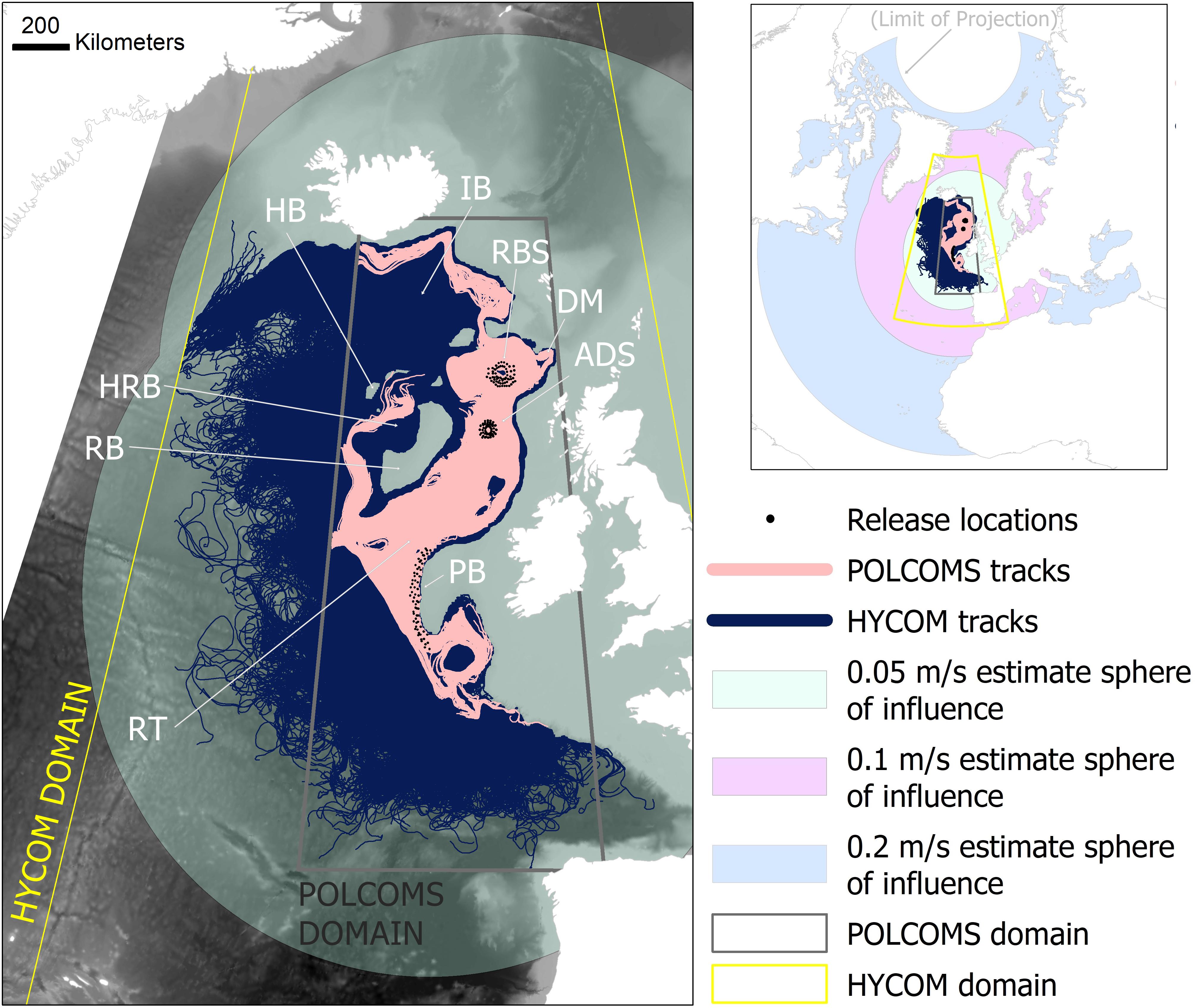
Figure 1. Labeled plots of the study area locations, together with all simulated tracks in the HYCOM and POLCOMS larval dispersal models relative to the smallest sphere of influence predictions of an average current speed based estimate (0.05 m/s; main map), and relative to all three current speed based estimates (0.05, 0.1, 0.2 m/s; inset). The gray and yellow boxes delineate the domain of the POLCOMS model and simulation domain of the HYCOM model, respectively. Tracks simulated by each model were unable to exit these areas. Quantitative comparisons were limited to the POLCOMS domain. The theoretical “larvae” were released from Rosemary Bank (RBS), Anton Dohrn Seamount (ADS), and Porcupine Bank (PB) (highlighted with red boxes). Features of topography mentioned in the text are labeled as follows: Iceland Basin (IB), Hatton Bank (HB), Darwin Mounds (DM), Hatton Rockall Basin (HRB), Rockall Bank (RB), Whittard Canyon (WC), Bay of Biscay (BB). [This map was created in ArcGIS 10.6.1 (http://www.esri.com) with GEBCO 30 arc-second topography, available from www.gebco.net, and projected using Albers Equal Area Conic with modified standard parallels and meridian (sp 1 = 46 °N, sp 2 = 61 °N, m = 13 °W)].

Estimate Calculation

This deep-sea case study relates findings to a figure published in McClain and Hardy (2010). The figure, notably with a caption full of caveats, displays potential larval dispersal distances of deep-sea fauna based on two different potential deep-sea averaged current speeds derived from Havenhand et al. (2005). This study will use a range of three possible average current speeds as the estimates, after Ellett et al. (1986) who observed vector-averaged current speeds (over 15 day periods between 1975 and 1982) of 0.1–0.2 m/s in the upper layers and 0.05 m/s at the deepest depths (>1750 m), as recorded in the vicinity of Anton Dohrn Seamount. Although this study is restricted to 700–1500 m depths, all three of these values (0.2, 0.1, 0.05 m/s) are tested for similarity to model-simulated dispersal, representing potential high, moderate, and low average current speeds. The 0.1 m/s estimate equates to the lower estimate in McClain and Hardy (2010).

LDMs

Two LDMs were run in this study, each consisting of a single particle simulator paired with one of the two hydrodynamic models; additional details on all model algorithms and parameterizations are available in Supplementary Material S1.

Particle Simulator: Connectivity Modeling System (CMS)

The CMS was used as the particle simulator (hereafter “simulator”) for both LDMs. There are many types of simulator available, but, without in-depth numerical modeling expertise, ecologists are likely to be limited to the use of offline simulators paired with the outputs from a hydrodynamic model (see Hilário et al.’s, 2015) supplementary table for a list of offline simulators and their compatibilities). The CMS is one such offline simulator. It is both freely available and designed especially with LDM in mind (v 1.1¹; Paris et al., 2013). This simulator has shown success in recent estimates of species connectivity (Wood et al., 2014; Ross et al., 2017; Baeza et al., 2019) as well as driving investigations of abyssal hydrodynamic transport (Van Sebille et al., 2013) among other studies.

While it is easy to integrate biological data, this study uses the simulator in its simplest configuration simulating passive dispersal for the cleanest comparison (and acting as a pre-cursor to later more complex biologically parameterized simulations). An hourly particle tracking timestep was used as decided by model sensitivity testing (Ross et al., 2016), and positional outputs were recorded daily.

Hydrodynamic Model 1: POLCOMS

POLCOMS is a shelf and coastal model used in United Kingdom and Irish waters. This version comes from Plymouth Marine Laboratory, United Kingdom. It was previously used by the United Kingdom Met Office in weather forecasting – a fact which might recommend it above other models in this area (Holt et al., 2001; Wakelin et al., 2009) and has been extensively validated over the United Kingdom surrounding waters (Holt et al., 2005). The 1/6°× 1/9° (c. 12 km²) resolution offers an eddy-resolving solution, however, it can only capture major eddies (c. 64 km in size based on needing six or more data points to adequately resolve an eddy; Lacroix et al., 2009) making this the coarser of the two models trialed. The model was run with 40 terrain following depth layers (sigma-levels) although outputs were interpolated to a z-level format (a list of set depth levels) using Matlab (v.R2013a) in order to make them compatible with the CMS. POLCOMS has been used in several dispersal studies to date (e.g., Lee et al., 2013; Phelps et al., 2015).

Hydrodynamic Model 2: HYCOM

HYCOM is a freely available global hydrodynamic model developed by the US Navy (Chassignet et al., 2007)². It is uniquely set up to use a hybrid of water mass following, terrain following, and depth specific vertical layers, changing with the underlying topography, which may make it well suited to deep-sea studies. The outputs, however, are in the z-level format required by the CMS (but may lose some of the hybrid grid details in the reformatting). The 1/12° resolution (c. 8 km × 4 km in the study area), allows smaller eddies (c. 48 km wide) to be captured than in POLCOMS, although this is still coarse relative to the multiple scales of oceanographic processes acting upon a larva. The global nature of HYCOM may be an upside for wide-ranging studies but is also a downside as the validation of the model was performed on a global scale and it may therefore not validate so well on a local scale (Fossette et al., 2012). HYCOM has already been used in multiple dispersal studies (Christie et al., 2010; Mora et al., 2011; Vasile et al., 2018), including in the deep-sea (Adams et al., 2011; Young et al., 2012; Ross et al., 2016, 2017).

Larval Releases

Theoretical “larvae” were released from three locations in the Rockall Trough in order to access different current regimes in the area: Rosemary Bank in the north, Anton Dohrn Seamount in the center, and Porcupine Bank in the south (see Supplementary Material S2 for exact positions). Releases were made from 16 positions per depth band from four depths (700, 1,000, 1,300, 1,500 m). Releases were made daily for 366 days from 4th January 2003 to 4th January 2004. All particles were tracked for 270 days in line with McClain and Hardy (2010), although daily positional outputs allow sub-setting of this PLD.

Simulations were run without additional subgrid-scale diffusivity parameters which would have added a random kick to particles at a regular timestep to represent unresolved small scale hydrodynamic processes. As this additional randomness would complicate interpretation of the difference in hydrodynamic model instruction, would require a different setting for each model, and would be subjectively chosen as a nest-wide parameter, these parameters were excluded from simulations. This decision is in line with the study undertaken by Shanks et al. (2003) in comparison to Siegel et al. (2003). As a result of excluding extra subgrid-scale diffusivity only one particle is released per day as simultaneous releases will follow identical tracks. Note, that, were this a species-specific study, we would advocate adding such subgrid-scale diffusivity parameters.

Neither of this study’s hydrodynamic models supply vertical velocity fields (w) due to their large spatial domains so simulations in this case are effectively 2-dimensional.

Analysis

In order to perform a comparison meaningful to ecologists and marine managers, both distance and spatial predictions were analyzed. Ecologists often examine dispersal kernels (a probability distribution of dispersal distances) and the potential distance of larval dispersal (terrestrial examples, Hovestadt et al., 2001; Baguette, 2003; Nathan, 2006; and marine examples, Siegel et al., 2003; Cowen et al., 2007; McClain and Hardy, 2010; Nickols et al., 2015), while marine managers may require more spatially explicit descriptions examining whether Location X is connected to Location Y (Treml and Halpin, 2012; Anadón et al., 2013; Puckett et al., 2014).

Distance Comparisons

Distance comparisons were illustrated by converting larval fates into effective dispersal kernels. CMS outputs consisting of daily positions of each simulated particle were converted into straight line distance (SLD) from source, per day, in Matlab (version R2013a) using the Haversine formula to account for earth curvature. A median SLD per day was then calculated for each model, as well as per depth per model, and associated quartiles. Note the median was selected, as opposed to the mean, as it is more robust in the presence of outlier values when sample size is large enough. The result was plotted against the average speed 0.1 m s^–1 line in the same format as the McClain and Hardy (2010) figure for ease of comparison.

The difference between SLDs was compared using repeated measures ANOVAs across time and within model-type to compute generalized effect sizes (η²_G) attributable to model differences (these are considered more valuable than p-values which can be overinflated for comparisons of model results; see White et al., 2014). In order to maintain balanced sample sizes, median SLDs represented the LDMs, together with the results from the slowest estimate (0.05 m/s) as it represents the prediction that is closest to the model simulations. Two ANOVAs were performed: one including all three methods (HYCOM, POLCOMS, Estimate), and another for the LDMs alone (HYCOM, POLCOMS), allowing the difference in generalized effect size (Δη²_G) to quantify the influence of the Estimate upon model effect in SLD predictions over time. Gamma GLMs (selected due to a continuous positive left-skewed distribution, and after extensive testing of model types and transformations) were used in tandem with the R function “drop1” to test whether the difference in 4th root transformed SLD per day was predominantly due to the effect of hydrodynamic model, rather than depth or location. These analyses were undertaken for the full 270 day time frame, with further reference points after 35 and 69 days tracking which were discerned by Hilário et al. (2015) as the median and 75% quartile PLDs of all deep-sea and eurybathic species, where PLD is currently known (n = 92 species).

Spatial Comparisons

Larval fates were mapped to offer a means of qualitative and quantitative spatial comparison. While some qualitative assessment is made on the full scale of these predictions (Figure 1), the majority of these analyses were restricted to the POLCOMS domain for fairer comparison (see Figure 1; the prediction area with the most restrictive boundaries).

Maps were created in ArcGIS (version 10.3) using an Albers Equal Area Conic Projection with modified standard parallels (46°N, 61°N). Quantitative comparisons are based on rasters with a grid of constant 4 km² cell size (approximately half the HYCOM model resolution), applied across the POLCOMS domain. For each depth band, grid cells occupied by topography were removed resulting in the 2D maximal possible area of occupancy.

The estimate spatial predictions were mapped as a sphere of influence buffer zones with radius equal to the predicted dispersal distance. The major limitation of an estimate prediction is that it cannot easily be extrapolated into a probabilistic spatial prediction without a method to quantify the error caused by assuming a constant current direction. All areas within the buffer zone were therefore considered as a presence-only record. All estimate predictions extended beyond the POLCOMS domain (see Figure 1) and could therefore always be considered equivalent to the full 2D maximal possible area of occupancy, when making comparison within this domain.

The prediction from each LDM was mapped as a percentage track density per grid cell occupancy in order to provide a spatial “heat map” of dispersal. To achieve this, Matlab was used to convert CMS outputs into ArcGIS-compatible subset.csv files for conversion into line shapefiles and subsequently density rasters. Track density values were used for the quantitative LDM comparison, while the estimate vs. model comparison required a binary (presence only) comparison of occupied cells.

A cumulative cell by cell linear correlation coefficient computed in R offers a single correlation value as representative of the comparison between each prediction (a raster correlation). This was performed per release location, per depth, and summarized as an average correlation between the LDM models and any of the three estimates within the POLCOMS domain.

Additional qualitative assessments offer real world interpretations of potential connectivity between sites. These are relevant to how usefully similar predictions may be to marine management and conservation.

Results

LDMs vs. Estimate

Both in terms of distance and spatial dispersal patterns, the estimate predictions were the least conservative and specific, with both modeled predictions being considerably more retentive and spatially targeted (Figures 1, 2).

FIGURE 2

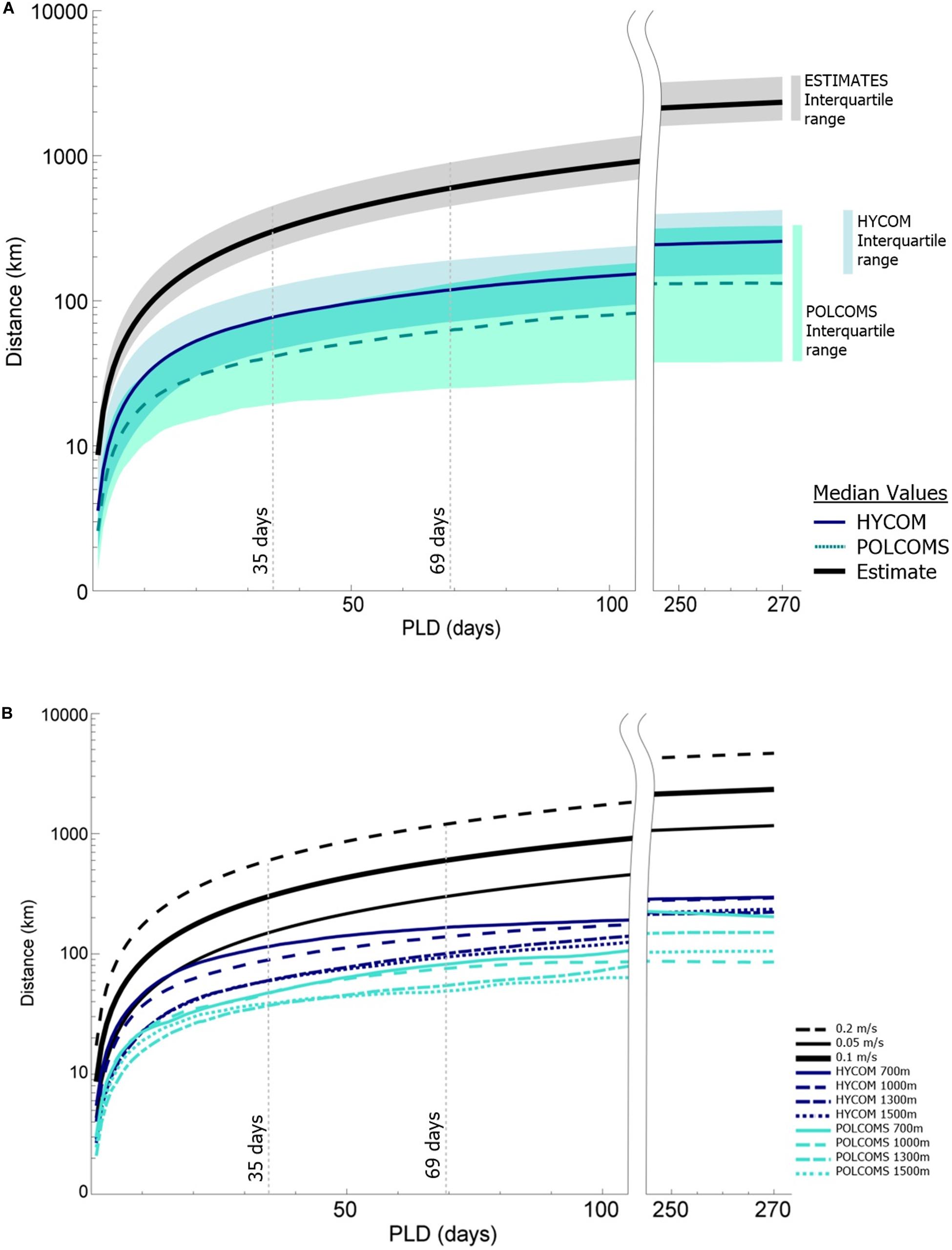
Figure 2. Results plots (after McClain and Hardy, 2010), of median dispersal distance over time for the model predictions as compared to the three estimates. (A) Median values per model (and the 0.1 m/s estimate) with shaded interquartile ranges inclusive of overlap. (B) Median values per depth band per model relative to the three estimates. Reference PLDs are highlighted in line with Hilário et al. (2015) and the PLDs representative of 50% (35 days) and 75% (69 days) of all known deep-sea animals.

Distance

Plots of median dispersal distance over time show a clear difference between the two LDM predictions and the range of estimates (Figure 2A). Tests of model type influence on SLD showed a 10–20% increase in variance explained, even when only the slowest estimate predictions (0.05 m/s) were included (Δη²_G, Table 1). The estimates offered the least conservative dispersal distances, being 1–7x the median LDM predicted dispersal distance from day one, scaling to 2–15x at 35 days, 2–19x at 69 days, and ending at 5–35x at the full 270 days tracking.

TABLE 1

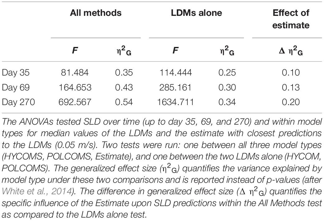
Table 1. Repeated measures ANOVA results.

However, there was reasonable convergence between the 0.05 m/s estimate and the HYCOM 700 simulation up until day 21 (Figure 2B), showing that estimates may still be useful for estimating dispersal distances for species with shorter PLDs.

Spatial – Correlation

The HYCOM LDM spatial predictions (as compared only within the POLCOMS domain) were the most similar to any estimate, although the similarity was still less than 0.5 (0.44 across all depths and locations; Table 2). The correlation between the estimates and POLCOMS LDM was very weak averaging 0.17 across all depths and locations. Across all depths and locations the correlation between estimated and modeled spatial extents was max. 0.67 (HYCOM LDM, Porcupine Bank, 700 m simulations), and min. 0.06 (POLCOMS LDM, Rosemary Bank, 1,500 m simulations).

TABLE 2

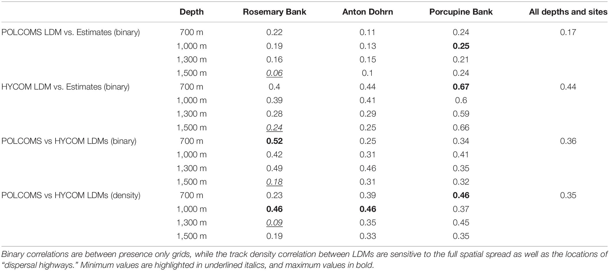
Table 2. Linear correlation coefficients between predictions provide quantitative spatial comparisons between LDM and estimate predictions.

Spatial – Qualitative

Qualitative spatial comparisons between the estimates and LDM predictions further emphasize the differences that could be encountered. Coarsely the 0.05 m/s estimate shows the greatest similarity to the LDM predictions (Figure 1), possibly being good enough if considering area of influence on the scale of the North Atlantic, but having an inadequate level of specificity to determine management measures within the study region.

However, if the faster estimates were to be chosen, then their spheres of influence, even considered on the scale of the North Atlantic, would be wildly different to LDM predictions (Figure 1, inset). The 0.1 m/s estimate would suggest a sphere of influence extending as far as North Africa, Svalbard, and Western Greenland, while the 0.2 m/s may suggest connections across the majority of the North Atlantic (Figure 1).

Focusing on the 0.05 m/s estimate (the estimate with the greatest similarity to the LDMs), the intra-study-region comparison between the estimate and each of the two LDMs separately, shows that POLCOMS LDM is the most different to the estimate. Even though the POLCOMS domain is the most restricted, there is a large area within that domain that remains untouched by POLCOMS dispersal pathways. For example, none of the POLCOMS releases connect to much of the Hatton Rockall Basin, the north side of Hatton Bank, or south beyond the Whittard Canyon in the Bay of Biscay (Figure 1).

Maps per model, location, and depth within the POLCOMS domain (Figures 3–5) allow visualization of more detailed comparisons. For example, Porcupine Bank simulations (Figure 5) suggesting no connection to Rosemary Bank at 1,300 and 1,500 m in either model, while even the 0.05 m/s estimate would comfortably make that distance. This would make a difference to a marine manager who might want to know whether known fauna at 1,500 m depth on Porcupine Bank can reach a protected area at Rosemary Bank: an estimate would say “yes,” and an LDM would say “no.”

FIGURE 3

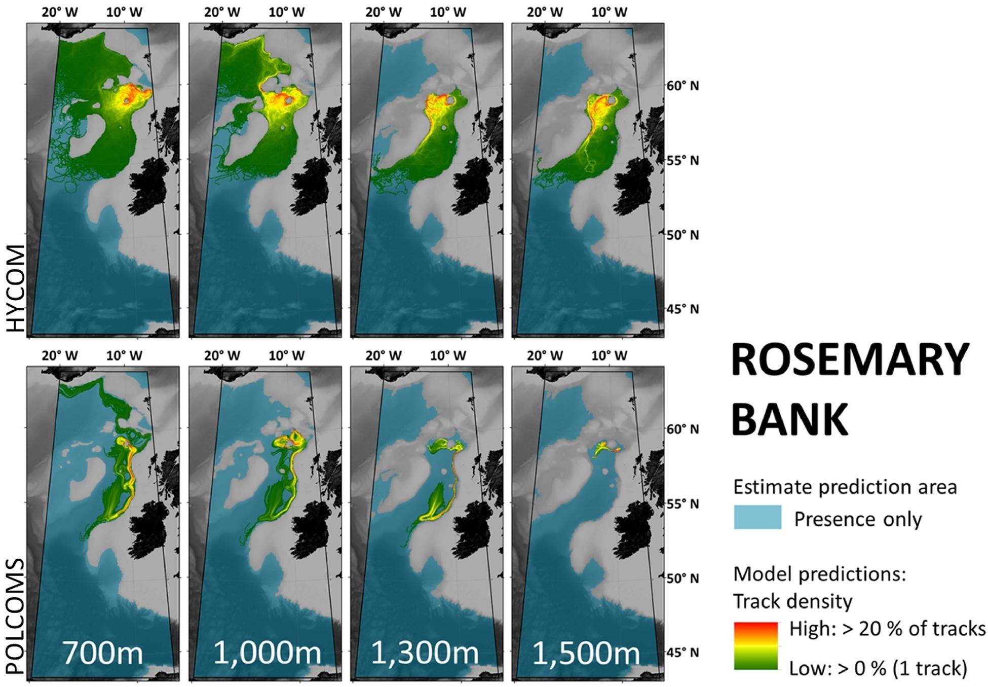
Figure 3. Maps per depth band of predicted larval dispersal as simulated from Rosemary Bank. Simulations from HYCOM and POLCOMS models are displayed as track densities delineating between occasional and persistent pathways of dispersal. All estimate prediction areas fill the POLCOMS domain but differ between maps due to the 2D nature of simulations excluding areas of raised topography. Spatial correlations were conducted comparing the extent of modeled and estimated predictions and the extent and density information of each modeled prediction (Table 2). [All maps were created in ArcGIS 10.3 (http://www.esri.com) with GEBCO 30 arc-second topography, available from www.gebco.net, and projected using Albers Equal Area Conic with modified standard parallels and meridian (sp 1 = 46 °N, sp 2 = 61 °N, m = 13 °W)].

Within the POLCOMS domain, the low correlation between any estimate and the POLCOMS LDM in particular can be exemplified by Figure 3. Here the estimate might expect connections between Rosemary Bank and anywhere in the Rockall Trough and Bay of Biscay to the south, while the POLCOMS LDM suggests that larvae may not even reach neighboring Rockall Bank in the west at any depth. Therefore, a marine manager asking whether there would be a dispersal connection between Rosemary Bank and Anton Dohrn Seamount would be told “yes” from an estimate, and “no” from a POLCOMS LDM.

HYCOM LDM vs. POLCOMS LDM

Generally, the two LDMs tested in this study give notably different predictions of dispersal, displaying differences in distance, spread, and, in some cases, direction of travel.

Distance

Figure 2A shows the lower median dispersal distances and much larger interquartile range of the POLCOMS predictions when compared to HYCOM (ANOVA η²_G = 0.25–0.34, i.e., 25–34% of variance is explained by model type between days 35 and 270, Table 1). GLMs confirmed that the effect of the model was greater than both depth and location for all PLDs tested (days 35, 69, and 270; see Supplementary Material S3, and bear in mind the advice of White et al., 2014). Plots of median dispersal distance per depth (Figure 2B) demonstrate that the shallowest (most dispersive) simulations in the POLCOMS model on average travel less far than the deepest (least dispersive) simulations in the HYCOM model.

Spatial – Correlation

The correlation between the track density maps of each LDM was generally low (Table 2, bottom section). The maximum correlation between POLCOMS and HYCOM simulations was 0.46 (Rosemary Bank 1,000 m; Anton Dohrn 1,000 m; and Porcupine Bank 700 m simulations), minimum 0.09 (Rosemary Bank 1,300 m simulations) and the average across all depths and locations only 0.35. This can be compared to the presence-only correlations which are also shown in Table 2 and are still low: max 0.52 (Rosemary Bank 700 m), min 0.18 (Rosemary Bank 1,500 m), av. 0.36.

Spatial – Qualitative

Generally, Rosemary Bank simulations were the most dissimilar (Figure 3). For example, while the 1,500 m Rosemary Bank simulations in HYCOM suggest connection southwards to most of the eastern flank of Rockall Bank, POLCOMS predicts a relatively small dispersal range suggesting there may be no connection to Rockall Bank at all.

Of most concern is when the two models disagree in the direction of dispersal. In Rosemary Bank 1,300 m simulations, HYCOM show the “highways” of high track density extending west down the eastern flank of Rockall Bank, while POLCOMS extends down the east of the Rockall Trough following the continental slope. Indeed in 1,000 m Rosemary Bank simulations, HYCOM larvae travel North, while POLCOMS larvae travel South.

By contrast, the results from Anton Dohrn Seamount (Figure 4) are more similar, with all “highways” generally extending north-east toward Rosemary Bank in both HYCOM and POLCOMS simulations. Yet if a marine manager were to ask whether larvae from Anton Dohrn reach the Darwin Mounds to the north-east, HYCOM would say “yes” and POLCOMS would say “no.”

FIGURE 4

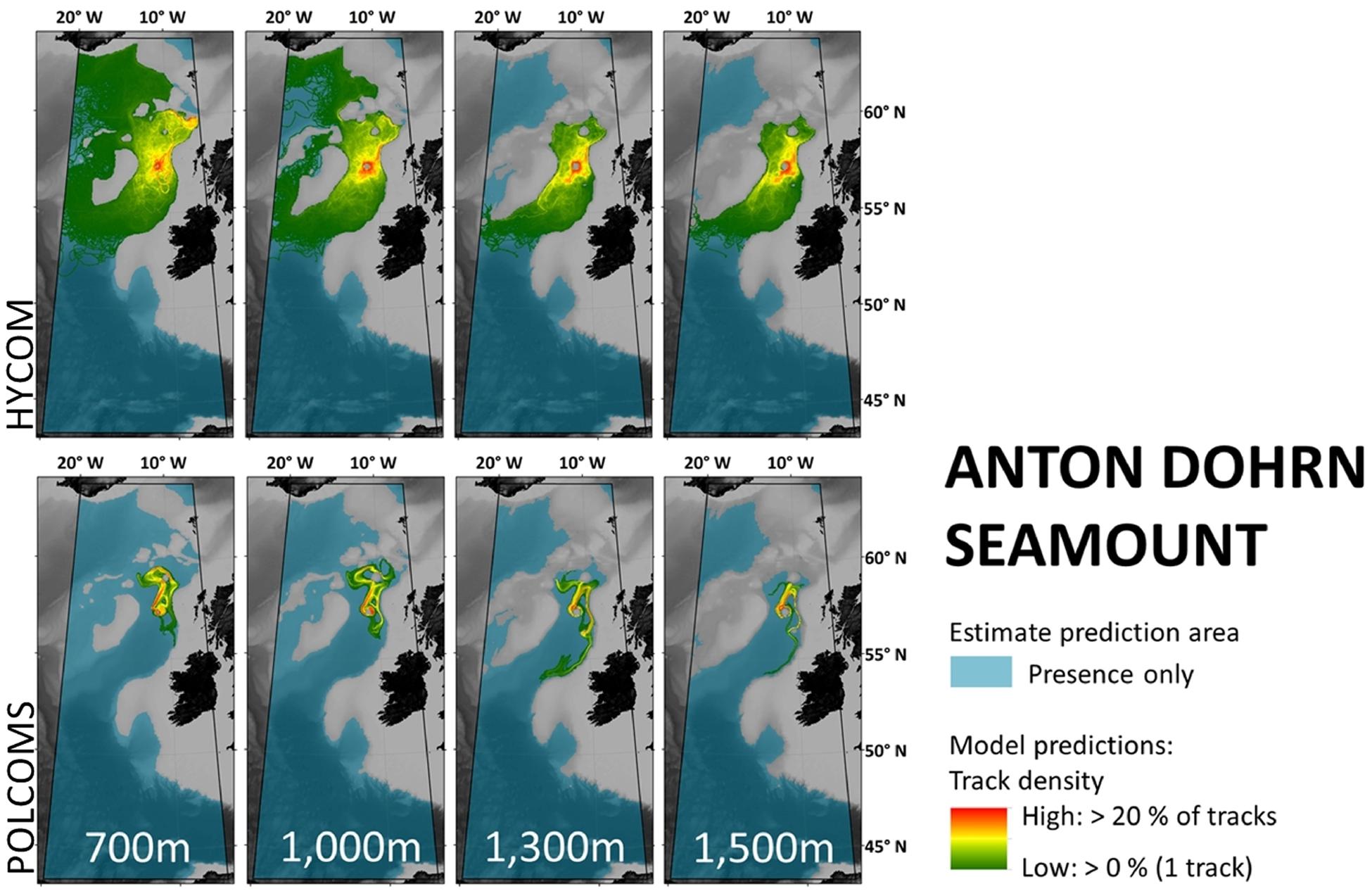
Figure 4. Maps per depth band of predicted larval dispersal as simulated from Anton Dohrn Seamount. Simulations from HYCOM and POLCOMS models are displayed as track densities delineating between occasional and persistent pathways of dispersal. All estimate prediction areas fill the POLCOMS domain but differ between maps due to the 2D nature of simulations excluding areas of raised topography. Spatial correlations were conducted comparing the extent of modeled and estimated predictions and the extent and density information of each modeled prediction (Table 2). [All maps were created in ArcGIS 10.3 (http://www.esri.com) with GEBCO 30 arc-second topography, available from www.gebco.net, and projected using Albers Equal Area Conic with modified standard parallels and meridian (sp 1 = 46 °N, sp 2 = 61 °N, m = 13 °W)].

Simulations from Porcupine Bank (Figure 5) might indicate a broad agreement that larvae will eventually reach the southern Rockall Bank, but the less direct “highways” in the POLCOMS model might reduce chances of larvae getting that far.

FIGURE 5

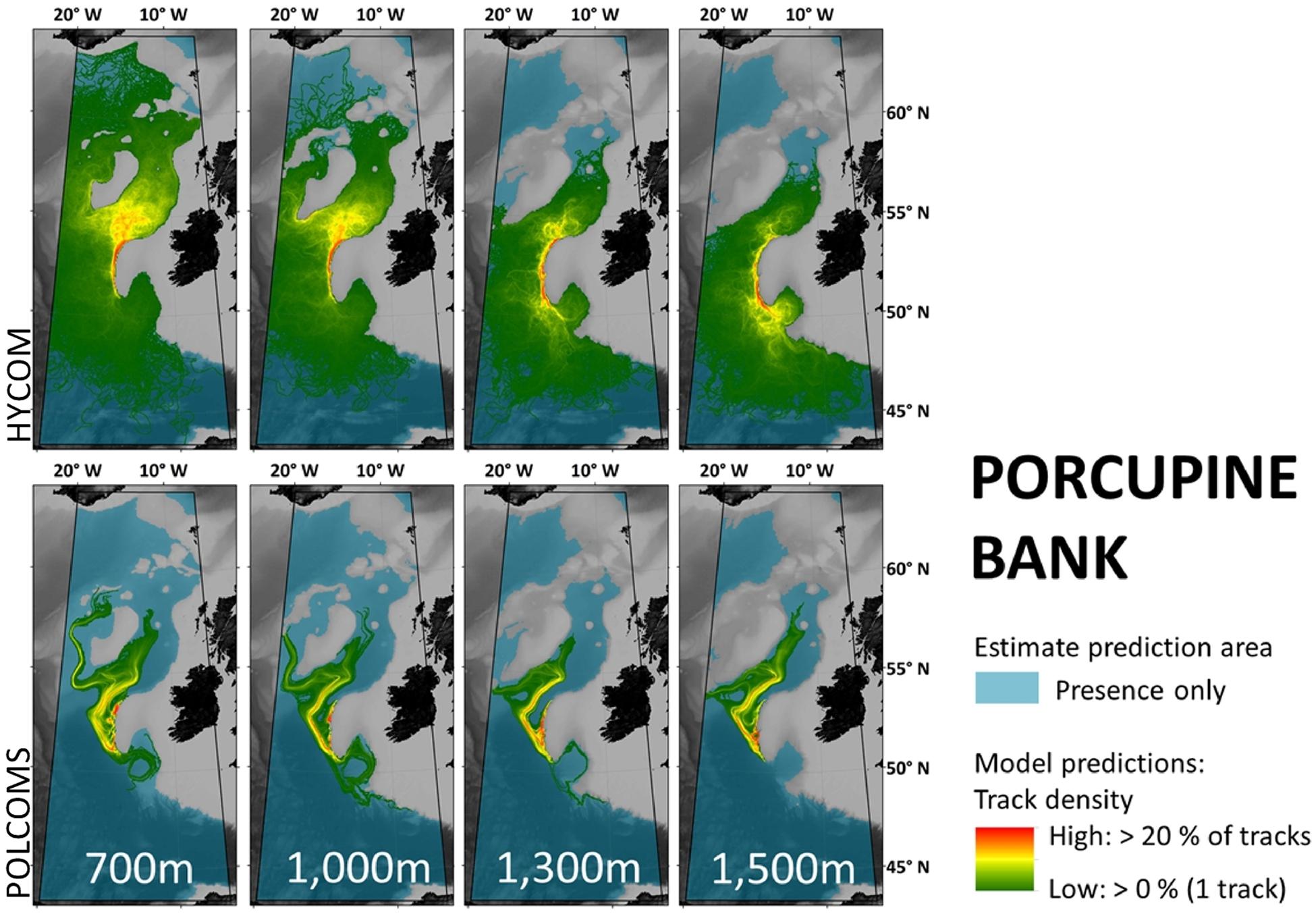
Figure 5. Maps per depth band of predicted larval dispersal as simulated from Porcupine Bank. Simulations from HYCOM and POLCOMS models are displayed as track densities delineating between occasional and persistent pathways of dispersal. All estimate prediction areas fill the POLCOMS domain but differ between maps due to the 2D nature of simulations excluding areas of raised topography. Spatial correlations were conducted comparing the extent of modeled and estimated predictions and the extent and density information of each modeled prediction (Table 2). [All maps were created in ArcGIS 10.3 (http://www.esri.com) with GEBCO 30 arc-second topography, available from www.gebco.net, and projected using Albers Equal Area Conic with modified standard parallels and meridian (sp 1 = 46 °N, sp 2 = 61 °N, m = 13 °W)].

Discussion

This study explored the value of larval dispersal predictions from LDMs by considering two questions.

Will LDMs Give a Notably Different Result to an (Informed) Estimate?

Our results agree with Shanks (2009) and suggest that yes, there can be a large difference in the predicted distance, area, and specificity of estimated and modeled dispersal patterns. There could therefore be a distinct advantage in going to the effort of modeling predictions, provided that models are shown to adequately approximate realistic distances better than the estimate. Although, were the study focus to be on a larger area (e.g., the North Atlantic, as mapped in Figure 1, inset), then the predictions given by a conservative estimate (here 0.05 m/s) and applied to sub-regions could be reasonably used to show local dispersal ranges.

One important note is to consider the range of current speed values we used for the estimates (as based on Ellett et al., 1986): the value with the greatest congruence to model simulations was the value least likely to be chosen to represent our study’s depth range. This study was focussed on depths between 700 and 1500 m so could reasonably have excluded the 0.05 m/s value which was recorded as the average for depths > 1750 m. The 0.1–0.2 m/s values that were associated with our studied depths showed vast overpredictions relative to the models, and highlights an issue of either gross overprediction from the estimates, or underprediction in the models. Only biological (genetic/geochemical) groundtruthing can provide “true” values to compare to, and these must be applied to species-specific models, not theoretical generalized models such as those undertaken here.

This study may also suggest that for deep-sea species the differences in predicted dispersal distance between models and estimates may be even more pronounced than in shallow water. As the divergence in predicted distance between estimates and models increased exponentially with tracking time (up to a maximum 34-fold difference, Figure 2), species with longer PLDs, such as those in the deep sea (Hilário et al., 2015), may show even greater disparity between estimated and modeled predictions.

However, there may have been better congruity between estimated and modeled predictions if simulations were undertaken in the open ocean. If any of the estimates were similar to the modeled predictions this would suggest that the model simulates currents with fairly straight trajectories and constant speeds: something more likely to occur on a relatively featureless abyssal plain at 5,000 m (but see Gardner et al., 2017). The complex topography of the Rockall Trough induces a lot of mesoscale activity (Holliday et al., 2000) which likely promotes greater local retention, and therefore differences in modeled predictions. Alternatively estimates could be made to better approximate what the models include; either by following the topography to account for the distance added by including depth, as is the case in 3D models, or by at least accounting for topographic barriers at the simulated depth, which would be a closer approximation to this study’s 2D simulations.

It is also important to mention that all the biological and ecological complexities (e.g., larval buoyancy, behavior, swimming speeds, growth, photo taxis, feeding methods, mortality, habitat selection, etc.) that can be simulated within an LDM, and that may have a large impact on larval dispersal patterns (Metaxas and Saunders, 2009), cannot necessarily be accounted for by using an estimate. These were excluded from the LDMs in this study, as they would only complicate the picture when trying to understand the impact of hydrodynamic model choice, but we absolutely advocate their inclusion in applied species-specific modeling studies and have done so in our own (e.g., Ross et al., 2017). On a coarse scale, inclusion of these characters in our LDMs may actually have increase the congruence with the slowest estimate, allowing larvae to bypass topographic barriers, potentially extending tracks north east toward Norway (see Ross et al., 2017). However, if focussed within our study region, again the specificity offered by an LDM may be of more value (again provided that those predictions are correct).

Are Two LDMs, Driven by Different Purpose-Selected Hydrodynamic Models, Cross-Validating, and Therefore of Some Value Prior to Targeted Groundtruthing?

Broadly, while some local comparisons may be cross-validating (e.g., in Anton Dohrn simulations), in this study the different hydrodynamic models also gave some contradictory predictions. Indeed, the variability in the predictions suggests that the potential for error within LDMs may be larger than previously recognized in ecology and conservation – a variability that cannot be apparent when modeling with only one hydrodynamic model. This result emphasizes that in all areas where the models disagree, there can be no trusted consensus until targeted groundtruthing takes place, and that the un-groundtruthed LDM outputs must not act as a basis for decision-makers before they have either been thoroughly assessed, or a groundtruthed consensus can be reached.

Broadly our result agrees with a comment from Bode et al. (2018) which showed that a re-run of a study by Hock et al. (2017) with an equivalent set up but using a different hydrodynamic model might have recommended different reefs for protection. They caution that biophysical models may be too immature to provide advisory results, and suggest that ensemble models may be a way to reach a conservative consensus in the meantime.

Model Differences

While we are not going to provide any criticism or endorsement for either model (as there are study-specific reasons for choosing one over another), we can offer some limited analysis and advice to aid model selection and interpretation in the future. Remember, however, that different applications may warrant different choices, even if your study is in the same region and depth range as ours.

In this case, there are three hydrodynamic model parameters that are worth highlighting and which may account for the differences in LDM predictions.

First, there are differences in the scales of validation between the models, but also in the relevance of these validations for dispersal modeling purposes. Despite both models being published and validated (Holt et al., 2001, 2005; Chassignet et al., 2007), HYCOM was assessed on a global scale and therefore may potentially be less locally reliable. However, neither model was validated for the purpose of larval dispersal modeling which may place greater weight on, for example, current directions and strengths than heat exchange and mixed-layer behavior. This makes it hard to use a model’s published validation status to judge whether the model is fit for purpose and recommends that study specific validation is vital, starting with a comparison to observational oceanography in the area (Vasile et al., 2018). In this study, for example, the southward trajectories of POLCOMS larvae down the eastern side of the Rockall Trough from Rosemary bank at 700–1,300 m (Figure 3) are contrary to the observations of northward transport down to 1,000 m, and below that southward transport down the western side of the Trough (Holliday and Cunningham, 2013; Holliday et al., 2015). However current speeds simulated in each model are different, with velocities in HYCOM being twice those in POLCOMS, although both fall within the range of observed current speeds recorded in the shelf edge current (10–21 cm s^–1) (White and Bowyer, 1997). Note that both models will suffer from many other errors including (but not limited to) currents that are too fast due to the exclusion of tides (Müller et al., 2010), coarse bathymetry that may exclude hydrographically influential features (Sandwell et al., 2014), and no representation of possible benthic storms which may divert dispersal pathways (Harris, 2014). Only targeted groundtruthing can quantify the error margins and clarify whether one model is more representative than the other for this purpose, and indeed they may each prove to have areas of accuracy at different depths or locations (Vasile et al., 2018).

Second, Spatial and temporal resolution has been shown to make a great difference in whether a model represents realistic trajectories or not. Putman and He (2013) advocate using the highest resolution model you can find, summarizing that model choice must aim to preserve physical processes on the scale tens of kilometers and days (respectively). Although both models may comply with this broad advice, HYCOM is still more highly resolved than POLCOMS. In this study area, while the major eddies may be over 100 km in diameter (Sherwin et al., 2015), there are still some influential semi-permanent features of 50–60 km in diameter (Booth, 1988; Ullgren and White, 2010). Given a rule-of-thumb that six data points are required to make an eddy (Lacroix et al., 2009), POLCOMS may omit these smaller eddies (min. eddy size of ∼64 km in diameter), while HYCOM may be capable of capturing them (min. ∼48 km in diameter). This difference in horizontal resolution may account for some of the difference in trajectory direction and tortuosity between the models. Consequently, we recommend that minimum resolution choice could be based on the size of permanent eddies in the study region (if that information is known).

Third, and possibly least obviously to ecologists, differing algorithms for error handling may be responsible for the more diffuse trajectories in the HYCOM model. The horizontal pressure gradient error stems from the issue of numerically interpreting flow around steep discretized (pixelated) topography and can result in perpetuated errors throughout the water column. This issue is handled in both models but using different approaches (see Supplementary Material S1 for model approaches). A representation of this can be seen in Supplementary Material S4, where plots of current ellipses per model, per depth, can help highlight these differences: the POLCOMS model shows less variable current direction and speed (smaller ellipses) and s tight shelf edge current, suggesting a stricter handling of these errors, and resulting in a less diffuse spread of particle trajectories. Accounting for this difference during model choice is more problematic for anyone who is not a numerical oceanographer, but highlighting its effect here may offer a means of recognition and inform interpretation of model predictions.

Groundtruthing

Groundtruthing should be regarded by all modelers as essential, and were the models found to be similar it would not have supplanted this necessity but could have lent some credence to modeled outputs before groundtruthing data became available. As it stands, however, the tested models could not be used interchangeably without consequence to ecological or marine management conclusions [e.g., whether Rosemary Bank was connected to south-east Rockall Bank at 1,300 m (Figure 3)]. Hence the next step must be to identify whether one model is more accurate than the other.

This study was entirely theoretical, for the purposes of hydrodynamic model comparison, and was therefore not tailored to any specific species (with biological characters as mentioned before). The only groundtruthing relevant to this study is therefore to use oceanographic observations. We have offered some provisional qualitative comparisons in section “Model Differences” but this could be taken further if truly assessing the hydrodynamic models, using chemical tracer data (e.g., Lavelle et al., 2010) and argo floats (e.g., Speer and Thurnherr, 2012). However, if this were a species-specific study then we would also have the option to undertake biological groundtruthing using sampled genetics or geochemical signatures [something that is rarely available but offers a next step for such studies (Levin, 2006)]. There majority of success stories to date have compared LDMs and seascape genetics (Foster et al., 2012; Sunday et al., 2014; Baeza et al., 2019).

Once groundtruthed, an LDM could be incredibly useful across disciplines and purposes, allowing subsequent simulations in the same region to be run and trusted for multiple species provided that similar oceanographic features are important to larval fates. New species predictions would then be able to rule out hydrodynamic sources of error leaving biological components as the main areas requiring groundtruthing in the future. It is therefore advisable to build the first species LDMs in a region upon the species with the greatest amount of data available for both model parameterization and groundtruthing. Once completed and tested, LDMs for other species can be created, safe in the knowledge that error due to hydrodynamic model choice is now quantified and controlled for.

Advice for Marine Managers and Ecologists

In this case, the variation in direction of dispersal makes it unwise to rely upon these predictions until they have been groundtruthed. However, were the differences only in speed and spread, these predictions may have been more useful, allowing interpretation relative to appropriate precautionary principles for the issue being considered. For example, MPA network design may wish to accommodate the most conservative predictions of dispersal to ensure that the larvae from a protected population can reach the next protected area (in this instance that would be POLCOMS predictions). Meanwhile if you were estimating invasive species spread, you may wish to default to a less conservative estimate (here HYCOM).

The variability between models also advocates the interpretation of LDM results as probabilistic (i.e., possible) rather than deterministic (i.e., true). Practically this may be translated as looking at the high density “highways of dispersal” which had some localized consensus between models, so these could be interpreted as the more likely pathways of dispersal, with lower density predictions being thought of as uncertain.

In summary, LDMs will have a place in marine ecology and conservation and offer a great improvement on informed estimates of dispersal potential, however, the hydrodynamic models they are based on can be very variable in their predictions, so should always be assumed to need some level of study-specific groundtruthing prior to relying upon predictions for management decisions and ecological theories. Utilizing local oceanographic observations and model comparisons can indeed offer some basic means of quantifying the uncertainty in model predictions to improve trust, but future comparison to population genetics, geochemical isotope tracers, or study-targeted groundtruthing data must still be considered essential.

Data Availability Statement

The datasets generated for this study are available on request to the corresponding author.

Author Contributions

KH and AN-S acquired the funding. RR, AN-S, and KH conceived the study. RT supplied the model data. RR analyzed the data. AN-S and KH provided advise and supervision. RR, AN-S, RT, and KH wrote the manuscript and interpreted the analysis.

Conflict of Interest

The authors declare that the research was conducted in the absence of any commercial or financial relationships that could be construed as a potential conflict of interest.

Funding

This work was funded by the United Kingdom Natural Environment Research Council on grant NE/K501104/1 which supported RR’s Ph.D. The Institute of Marine Research (IMR/Havforskningsinstituttet), Norway supported RR as a post doc to complete this work and funded the open access fee for this publication. RT was supported by UK Research and Innovation National Environmental Research Council (UKRI-NERC) National Capability funding program CLASS (NE/R015953/1).

Acknowledgments

We would like to thank Plymouth Marine Laboratory for supplying outputs from the POLCOMS model; Nataliya Stashchuk for assistance in interpolating POLCOMS from sigma to z-level format; Peter Mills and Antonio Rago for High Performance Computing support; Vasyl Vlasenko for his supervision; and Antony Knights, John Spicer, and Anthony Grehan for their advice and guidance, and multiple reviewers and editors for their time and suggestions which have greatly improved this manuscript. RR would also like to credit an article by Kevin Plaxco for informing all the best aspects of how this manuscript is written (Plaxco, 2010). This manuscript has been released as a Pre-Print at BioRxiv.org (Ross et al., 2019; https://doi.org/10.1101/599696).

Supplementary Material

The Supplementary Material for this article can be found online at: https://www.frontiersin.org/articles/10.3389/fmars.2020.00431/full#supplementary-material

Footnotes

1. ^ https://github.com/beatrixparis/connectivity-modeling-system
2. ^ www.hycom.org

References

Adams, D. K., McGillicuddy, D. J. Jr., Zamudio, L., Thurnherr, A. M., Liang, X., Rouxel, O., et al. (2011). Surface-generated mesoscale eddies transport deep-sea products from hydrothermal vents. Science 332, 580–583. doi: 10.1126/science.1201066

PubMed Abstract | CrossRef Full Text | Google Scholar

Aleynik, D., Adams, T., Davidson, K., Dale, A., Porter, M., Black, K., et al. (2018). “Biophysical modelling of marine organisms: fundamentals and applications to management of coastal waters,” in Environmental Management of Marine Ecosystems, eds M. N. Islam and S. E. Jorgensen (Boca Raton: CRC Press), 65–98. doi: 10.1201/9781315153933-3

CrossRef Full Text | Google Scholar

Anadón, J. D., del Mar Mancha-Cisneros, M., Best, B. D., and Gerber, L. R. (2013). Habitat-specific larval dispersal and marine connectivity: implications for spatial conservation planning. Ecosphere 4:82. doi: 10.1890/ES13-00119.1

CrossRef Full Text | Google Scholar

Baeza, J. A., Holstein, D., Umaña-Castro, R., and Mejía-Ortíz, L. M. (2019). Population genetics and biophysical modelling inform metapopulation connectivity of the Caribbean king crab Maguimithrax spinosissimus. Mar. Ecol. Prog. Ser. 610, 83–97. doi: 10.3354/meps12842

CrossRef Full Text | Google Scholar

Baguette, M. (2003). Long distance dispersal and landscape occupancy in a metapopulation of the cranberry fritillary butterfly. Ecography 26, 153–160. doi: 10.1034/j.1600-0587.2003.03364.x

PubMed Abstract | CrossRef Full Text | Google Scholar

Bode, M., Bode, L., Choukroun, S., James, M. K., and Mason, L. B. (2018). Resilient reefs may exist, but can larval dispersal models find them? PLoS Biol. 16:e2005964. doi: 10.1371/journal.pbio.2005964

PubMed Abstract | CrossRef Full Text | Google Scholar

Booth, D. (1988). Eddies in the rockall trough. Oceanol. acta 11, 213–219.

Google Scholar

Chassignet, E. P., Hurlburt, H. E., Smedstad, O. M., Halliwell, G. R., Hogan, P. J., Wallcraft, A. J., et al. (2007). The HYCOM (HYbrid Coordinate Ocean Model) data assimilative system. J. Mar. Sys. 65, 60–83.

Google Scholar

Christie, M. R., Tissot, B. N., Albins, M. A., Beets, J. P., Jia, Y., Ortiz, D. M., et al. (2010). Larval connectivity in an effective network of marine protected areas. PLoS One 5:e15715. doi: 10.1371/journal.pone.0015715

PubMed Abstract | CrossRef Full Text | Google Scholar

Cowen, R. K., Gawarkiewicz, G., Pineda, J., Thorrold, S. R., and Werner, F. E. (2007). Population connectivity in marine systems: an overview. Oceanography 20, 14–21. doi: 10.5670/oceanog.2007.26

CrossRef Full Text | Google Scholar

Elith, J., and Graham, C. H. (2009). Do they? How do they? WHY do they differ? on finding reasons for differing performances of species distribution models. Ecography 32, 66–77. doi: 10.1111/j.1600-0587.2008.05505.x

CrossRef Full Text | Google Scholar

Ellett, D. J., Edwards, A., and Bowers, R. (1986). The hydrography of the Rockall Channel—an overview. Proc. R. Soc. Edinburgh. Sect. B. Biol. Sci. 88, 61–81. doi: 10.1017/s0269727000004474

CrossRef Full Text | Google Scholar

Fossette, S., Putman, N., Lohmann, K., Marsh, R., and Hays, G. (2012). A biologist’s guide to assessing ocean currents: a review. Mar. Ecol. Prog. Ser. 457, 285–301. doi: 10.3354/meps09581

CrossRef Full Text | Google Scholar

Foster, N. L., Paris, C. B., Kool, J. T., Baums, I. B., Stevens, J. R., Sanchez, J. A., et al. (2012). Connectivity of Caribbean coral populations: complementary insights from empirical and modelled gene flow. Mol. Ecol. 21, 1143–1157. doi: 10.1111/j.1365-294x.2012.05455.x

PubMed Abstract | CrossRef Full Text | Google Scholar

Gardner, W. D., Tucholke, B. E., Richardson, M. J., and Biscaye, P. E. (2017). Benthic storms, nepheloid layers, and linkage with upper ocean dynamics in the western North Atlantic. Mar. Geol. 385, 304–327. doi: 10.1016/j.margeo.2016.12.012

CrossRef Full Text | Google Scholar

Harris, P. T. (2014). Shelf and deep-sea sedimentary environments and physical benthic disturbance regimes: a review and synthesis. Mar. Geol. 353, 169–184. doi: 10.1016/j.margeo.2014.03.023

CrossRef Full Text | Google Scholar

Havenhand, J. N., Matsumoto, G. I., and Sidel, E. (2005). Megalodicopia hians in the Monterey submarine canyon: distribution, larval development, and culture. Deep Sea Res. Part I Oceanogr. Res. Pap 53, 215–222. doi: 10.1016/j.dsr.2005.11.005

CrossRef Full Text | Google Scholar

Hilário, A., Metaxas, A., Gaudron, S. M., Howell, K. L., Mercier, A., Mestre, N. C., et al. (2015). Estimating dispersal distance in the deep sea: challenges and applications to marine reserves. Front. Mar. Sci. 2:6. doi: 10.3389/fmars.2015.00006

CrossRef Full Text | Google Scholar

Hock, K., Wolff, N. H., Ortiz, J. C., Condie, S. A., Anthony, K. R., et al. (2017). Connectivity and systemic resilience of the Great Barrier Reef. PLoS Biol. 15:e2003355. doi: 10.1371/journal.pbio.2003355

PubMed Abstract | CrossRef Full Text | Google Scholar

Holliday, N. P., Cunningham, S. A., Johnson, C., Gary, S. F., Griffiths, C., Read, J. F., et al. (2015). Multidecadal variability of potential temperature, salinity, and transport in the eastern subpolar North Atlantic. J. Geophys. Res. Ocean. 120, 1–23.

Google Scholar

Holliday, N. P., Pollard, R. T., Read, J. F., and Leach, H. (2000). Water mass properties and fluxes in the Rockall Trough, 1975-1998. Deep Sea Res. Part I Oceanogr. Res. Pap. 47, 1303–1332. doi: 10.1016/s0967-0637(99)00109-0

CrossRef Full Text | Google Scholar

Holliday, P., and Cunningham, S. (2013). The extended ellett line: discoveries from 65 years of marine observations west of the UK. Oceanography 26, 156–163.

Google Scholar

Holt, J. T., Allen, J. I., Proctor, R., and Gilbert, F. (2005). Error quantification of a high resolution coupled hydrodynamic-ecosystem coastal-ocean model: part 1 model overview and assessment of the hydrodynamics. J. Mar. Sys. 57, 167–188. doi: 10.1016/j.jmarsys.2005.04.008

CrossRef Full Text | Google Scholar

Holt, J. T., James, I. D., and Jones, J. E. (2001). An s coordinate density evolving model of the northwest European continental shelf 2, seasonal currents and tides. J. Geophys. Res. 106, 14035–14053. doi: 10.1029/2000jc000303

CrossRef Full Text | Google Scholar

Hovestadt, T., Messner, S., and Poethke, H. J. (2001). Evolution of reduced dispersal mortality and “fat-tailed” dispersal kernels in autocorrelated landscapes. Proc. Biol. Sci. 268, 385–391. doi: 10.1098/rspb.2000.1379

PubMed Abstract | CrossRef Full Text | Google Scholar

Kenchington, E., Wang, Z., Lirette, C., Murillo, F. J., Guijarro, J., Yashayaev, I., et al. (2019). Connectivity modelling of areas closed to protect vulnerable marine ecosystems in the northwest Atlantic. Deep Sea Res. Part I Oceanogr. Res. Pap 143, 85–103. doi: 10.1016/j.dsr.2018.11.007

CrossRef Full Text | Google Scholar

Lacroix, G., McCloghrie, P., Huret, M., and North, E. (2009). “Hydrodynamic models,” in Manual of Recommended Practices for Modelling Physical-Biological Interactions During Early Fish Life, eds E. W. North, A. Gallego, and P. Pettigas (Toronto, ON: ICES), 3–8.

Google Scholar

Lavelle, J. W., Thurnherr, A. M., Ledwell, J. R., McGillicuddy, D. J. Jr., and Mullineaux, L. S. (2010). Deep ocean circulation and transport where the East Pacific Rise at 9–10°N meets the Lamont seamount chain. J. Geophys. Res. 115:1163.

Google Scholar

Lee, P. L. M., Dawson, M. N., Neill, S. P., Robins, P. E., Houghton, J. D. R., Doyle, T. K., et al. (2013). Identification of genetically and oceanographically distinct blooms of jellyfish. J. R. Soc. Interface 10:20120920. doi: 10.1098/rsif.2012.0920

PubMed Abstract | CrossRef Full Text | Google Scholar

Levin, L. A. (2006). Recent progress in understanding larval dispersal: new directions and digressions. Integr. Comp. Biol. 46, 282–297. doi: 10.1093/icb/icj024

PubMed Abstract | CrossRef Full Text | Google Scholar

McClain, C. R., and Hardy, S. M. (2010). The dynamics of biogeographic ranges in the deep sea. Proc. R. Soc. London B Biol. Sci. 277, 3533–3546. doi: 10.1098/rspb.2010.1057

PubMed Abstract | CrossRef Full Text | Google Scholar

Metaxas, A., and Saunders, M. (2009). Quantifying the “Bio-” components in biophysical models of larval transport in marine benthic invertebrates: advances and pitfalls. Biol. Bull. 216, 257–272. doi: 10.1086/bblv216n3p257

PubMed Abstract | CrossRef Full Text | Google Scholar

Mora, C., Treml, E. A., Roberts, J., Crosby, K., Roy, D., and Tittensor, D. P. (2011). High connectivity among habitats precludes the relationship between dispersal and range size in tropical reef fishes. Ecography 35, 89–96. doi: 10.1111/j.1600-0587.2011.06874.x

CrossRef Full Text | Google Scholar

Müller, M., Haak, H., Jungclaus, J. H., Sündermann, J., and Thomas, M. (2010). The effect of ocean tides on a climate model simulation. Ocean Model. 35, 304–313. doi: 10.1016/j.ocemod.2010.09.001

CrossRef Full Text | Google Scholar

Nathan, R. (2006). Long-distance dispersal of plants. Science 313, 786–788. doi: 10.1126/science.1124975

PubMed Abstract | CrossRef Full Text | Google Scholar

Nickols, K. J., White, J. W., Largier, J. L., and Gaylord, B. (2015). Marine population connectivity: reconciling large-scale dispersal and high self-retention. Am. Nat. 185, 196–211. doi: 10.1086/679503

PubMed Abstract | CrossRef Full Text | Google Scholar

North, E. W., Gallego, A., and Pettigas, P. (2009). Manual of Recommended Practices for Modelling Physical-Biological Interactions During Early Fish Life. Toronto, ON: ICES, 1–111.

Google Scholar

Paris, C. B., Helgers, J., van Sebille, E., and Srinivasan, A. (2013). Connectivity modeling system: a probabilistic modeling tool for the multi-scale tracking of biotic and abiotic variability in the ocean. Environ. Model. Softw. 42, 47–54. doi: 10.1016/j.envsoft.2012.12.006

CrossRef Full Text | Google Scholar

Phelps, J., Polton, J., Souza, A., and Robinson, L. (2015). Behaviour influences larval dispersal in shelf sea gyres: Nephrops norvegicus in the Irish Sea. Mar. Ecol. Prog. Ser. 518, 177–191. doi: 10.3354/meps11040

CrossRef Full Text | Google Scholar

Piechaud, N., Downie, A., Stewart, H. A., and Howell, K. L. (2015). The impact of modelling method selection on predicted extent and distribution of deep-sea benthic assemblages. Earth Environ. Sci. Trans. R. Soc. Edinburgh 105, 251–261. doi: 10.1017/s1755691015000122

CrossRef Full Text | Google Scholar

Plaxco, K. W. (2010). The art of writing science. Protein Sci. 19, 2261–2266. doi: 10.1002/pro.514

PubMed Abstract | CrossRef Full Text | Google Scholar

Puckett, B. J., Eggleston, D. B., Kerr, P. C., and Luettich, R. A. (2014). Larval dispersal and population connectivity among a network of marine reserves. Fish. Oceanogr. 23, 342–361. doi: 10.1111/fog.12067

CrossRef Full Text | Google Scholar

Putman, N. F., and He, R. (2013). Tracking the long-distance dispersal of marine organisms: sensitivity to ocean model resolution. J. R. Soc. Interface 10:20120979. doi: 10.1098/rsif.2012.0979

PubMed Abstract | CrossRef Full Text | Google Scholar

Roberts, C. M., Andelman, S., Branch, G., Bustamante, R. H., Castilla, J. C., Dugan, J., et al. (2003). Ecological criteria for evaluating candidate sites for marine reserves. Ecol. App. 13, 199–214. doi: 10.1890/1051-0761(2003)013[0199:ecfecs]2.0.co;2

CrossRef Full Text | Google Scholar

Roberts, C. M., Hawkins, J. P., Fletcher, J., Hands, S., Raab, K., and Ward, S. (2010). Guidance on the Size and Spacing of Marine Protected Areas in England. York: Natural England, 1–87.

Google Scholar

Ross, R. E., Nimmo-Smith, W. A. M., and Howell, K. L. (2016). Increasing the depth of current understanding: sensitivity testing of deep-sea larval dispersal models for ecologists. PLoS One 11:e0161220. doi: 10.1371/journal.pone.0161220

PubMed Abstract | CrossRef Full Text | Google Scholar

Ross, R. E., Nimmo-Smith, W. A. M., and Howell, K. L. (2017). Towards ‘ecological coherence’: assessing larval dispersal within a network of existing Marine Protected Areas. Deep Sea Res. Part I Oceanogr. Res. Pap. 126, 128–138. doi: 10.1016/j.dsr.2017.06.004

CrossRef Full Text | Google Scholar

Ross, R. E., Nimmo-Smith, W. A. M., Torres, T., and Howell, K. L. (2019). Modelling marine larval dispersal: a cautionary deep-sea tale for ecology and conservation. bioRxiv[Preprint] doi: 10.1101/599696

CrossRef Full Text | Google Scholar

Sandwell, D. T., Müller, R. D., Smith, W. H. F., Garcia, E., and Francis, R. (2014). New global marine gravity model from CryoSat-2 and Jason-1 reveals buried tectonic structure. Science 346, 65–67. doi: 10.1126/science.1258213

PubMed Abstract | CrossRef Full Text | Google Scholar

Shanks, A. L. (2009). Pelagic larval duration and dispersal distance revisited. Biol. Bull. 216, 373–385. doi: 10.1086/bblv216n3p373

PubMed Abstract | CrossRef Full Text | Google Scholar

Shanks, A. L., Grantham, B. A., and Carr, M. H. (2003). Propagule dispersal distance and the size and spacing of marine reserves. Ecol. Appl. 13, S159–S169.

Google Scholar

Sherwin, T. J., Aleynik, D., Dumont, E., and Inall, M. E. (2015). Deep drivers of mesoscale circulation in the central Rockall Trough. Ocean Sci. 11, 343–359. doi: 10.5194/os-11-343-2015

CrossRef Full Text | Google Scholar

Siegel, D. A., Kinlan, B. P., Gaylord, B., and Gaines, S. D. (2003). Lagrangian descriptions of marine larval dispersion. Mar. Ecol. Prog. Ser. 260, 83–96. doi: 10.3354/meps260083

CrossRef Full Text | Google Scholar

Speer, K., and Thurnherr, A. M. (2012). The lau basin float experiment (LAUB-FLEX). Oceanography 25, 284–285. doi: 10.5670/oceanog.2012.27

CrossRef Full Text | Google Scholar

Sunday, J. M., Popovic, I., Palen, W. J., Foreman, M. G. G., and Hart, M. W. (2014). Ocean circulation model predicts high genetic structure observed in a long-lived pelagic developer. Mol. Ecol. 23, 5036–5047. doi: 10.1111/mec.12924

PubMed Abstract | CrossRef Full Text | Google Scholar

Treml, E. A., and Halpin, P. N. (2012). Marine population connectivity identifies ecological neighbors for conservation planning in the Coral Triangle. Conserv. Lett. 5, 441–449. doi: 10.1111/j.1755-263x.2012.00260.x

CrossRef Full Text | Google Scholar

Ullgren, J. E., and White, M. (2010). Water mass interaction at intermediate depths in the southern rockall trough, northeastern North Atlantic. Deep. Sea. Res. Part I Oceanogr. Res. Pap. 57, 248–257. doi: 10.1016/j.dsr.2009.11.005

CrossRef Full Text | Google Scholar

Van Sebille, E., Spence, P., Mazloff, M. R., England, M. H., Rintoul, S. R., and Saenko, O. A. (2013). Abyssal connections of Antarctic bottom water in a southern ocean state estimate. Geophys. Res. Lett. 40, 2177–2182. doi: 10.1002/grl.50483

CrossRef Full Text | Google Scholar

Vasile, R., Hartmann, K., Hobday, A. J., Oliver, E., and Tracey, S. (2018). Evaluation of hydrodynamic ocean models as a first step in larval dispersal modelling. Cont. Shelf Res. 152, 38–49. doi: 10.1016/j.csr.2017.11.001

CrossRef Full Text | Google Scholar

Wakelin, S. L., Holt, J. T., and Proctor, R. (2009). The influence of initial conditions and open boundary conditions on shelf circulation in a 3D ocean-shelf model of the north east Atlantic. Ocean Dyn. 59, 67–81. doi: 10.1007/s10236-008-0164-3

CrossRef Full Text | Google Scholar

Werner, F., Cowen, R., and Paris, C. (2007). Coupled biological and physical models: present capabilities and necessary developments for future studies of population connectivity. Oceanography 20, 54–69. doi: 10.5670/oceanog.2007.29

CrossRef Full Text | Google Scholar

White, J. W., Rassweiler, A., Samhouri, J. F., Stier, A. C., and White, C. (2014). Ecologists should not use statistical significance tests to interpret simulation model results. Oikos 123, 385–388. doi: 10.1111/j.1600-0706.2013.01073.x

CrossRef Full Text | Google Scholar

White, M., and Bowyer, P. (1997). The shelf-edge current north-west of Ireland. Ann. Geophysicae 15, 1076–1083. doi: 10.1007/s00585-997-1076-0

CrossRef Full Text | Google Scholar

Wood, S., Paris, C. B., Ridgwell, A., and Hendy, E. J. (2014). Modelling dispersal and connectivity of broadcast spawning corals at the global scale. Glob. Ecol. Biogeogr. 23, 1–11. doi: 10.1111/geb.12101

CrossRef Full Text | Google Scholar

Young, C. M., He, R., Emlet, R. B., Li, Y., Qian, H., Arellano, S. M., et al. (2012). Dispersal of deep-sea larvae from the intra-American seas: simulations of trajectories using ocean models. Integr. Comput. Biol. 52, 483–496. doi: 10.1093/icb/ics090

PubMed Abstract | CrossRef Full Text | Google Scholar