Persistent Hydrodynamic Cues Elicit Orientation-Specific Behavioral Sensitivities and Kinematic Responses in Dispersed Crab Larvae

1. Introduction

Dispersal trajectories of pelagic zooplankton are fundamentally influenced by both individual behavior and physical forcing (Woodson and McManus, 2007). For Brachyuran crabs whose life history includes a dispersed larval stage preceding benthic settlement, a predominant behavioral mode is depth-regulation that enables diel, tidal (endogenous), and ontogenetic (larval stage-specific) vertical migrations. Well-timed vertical migrations allow larvae to exploit vertical gradients of horizontal velocity, typical in nearshore and estuarine hydrodynamics (Figure 1), in order to selectively induce horizontal transport and improve fitness through favorable habitat selection. For example, larvae can gain net transport shoreward by swimming vertically down during ebb tide and up during flood tide. Or, depending on the goals of the particular larval stage, they can gain net transport seaward with the opposite behavior. These behavioral adaptations are collectively referred to as selective tidal stream transport (STST), and they strongly affect dispersal trajectories and population connectivity (Cronin and Forward, 1986; Eggleston et al., 1998; Forward et al., 2001, 2004).

FIGURE 1

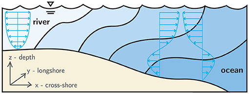
Figure 1. Conceptual schematic of estuarine hydrodynamics. Shades of blue indicate water masses of differing salinity in a weakly-stratified estuary, and the blue arrows indicate tidally-modulated, oscillating flow structure.

There are a number of environmental cues that strongly affect larval swimming behaviors throughout dispersal (Ott and Forward, 1976; Queiroga and Blanton, 2005; Lecchini et al., 2010). Vertical migratory behaviors and depth-regulation are predominant behavioral responses driven by combined geotaxis, phototaxis, and barokinesis (Forward, 1974; Sulkin, 1975, 1984; Sulkin et al., 1980). Other larval behavioral responses to environmental cues are strongly dependent on larval stage (Shanks, 1986; Jamieson and Phillips, 1988; Hobbs and Botsford, 1992) and the particular combination of cues present (Queiroga and Blanton, 2005), as well as their intensities (Tankersley et al., 1995) and rates of change (Forward, 1989a). Nonetheless, some larval stage-specific behavioral patterns emerge. For example, megalopae (the post-larval stage directly preceding benthic settlement) respond to increasing pressure (Forward, 1990), salinity (Queiroga and Blanton, 2005), and turbulent kinetic energy (Welch et al., 1999) associated with flood tide by swimming vertically upward to induce shoreward transport toward favorable benthic settlement habitats (flood tide transport, FTT). However, these typical behavioral responses may be confounded by finescale foraging and sampling behaviors induced by chemical and hydrodynamic cues indicative of nearby resource patches. The intermittent presence of a dominant sensory cue that induces localized foraging and sampling may cause temporary departures from typical behavioral modes such as FTT and significantly influence larval dispersal trajectories (Woodson and McManus, 2007).

Effective foraging and sampling behaviors in competent larval stages are enabled by highly-developed morphologies suitable for detecting and exploiting ambient chemical and hydrodynamic cues (Anger, 2001; Queiroga and Blanton, 2005). Chemical cues can induce or delay larval metamorphoses (Rodriguez and Epifanio, 2000; Andrews et al., 2001), inform habitat selection (Forward et al., 2001; Lecchini et al., 2010; Tapia-Lewin and Pardo, 2014), and affect swimming behaviors (Forward et al., 2003a; Houser and Epifanio, 2009). Further, hydrodynamic cues associated with fluid velocity gradients fundamentally structure complex estuarine and nearshore environments. Hydrodynamic cues that mechanosensitive larvae may respond to, in any flow of interest, include rotation (vorticity), deformation (strain), and acceleration, which follows directly from the total or material derivative of the fluid velocity field in the Navier-Stokes equations that govern fluid motion. The material derivative includes the temporal (unsteady) acceleration term as well as the spatial (convective) acceleration terms resulting from the dot product of the velocity vector and the velocity gradient tensor; the decomposition of this tensor, in turn, yields the fluid deformation rate and rotation rate tensors (Kundu et al., 2011). Larvae may respond to all or any of these hydrodynamic cues, for example, when exposed to turbulent flow. Changing turbulent kinetic energy (TKE) levels elicits excited swimming (Welch et al., 1999) that enhances effective STST (Criales et al., 2013), one of the most distinctive behavioral modes of dispersed larvae.

While it is well-understood that turbulence, with its characteristic unsteadiness and rapidly fluctuating hydrodynamic cues, plays an important role in larval behavior (Queiroga and Blanton, 2005), the potential relevance of hydrodynamic cues associated with spatiotemporally persistent flow features remains largely unknown, despite the fact that such cues are likely to be ecologically relevant. Finescale hydrographic structure in the water column is often associated with enhanced productivity and high-density resource patches, such as the regions around fronts and clines (Largier, 1993; McManus et al., 2003). This suggests that spatiotemporally persistent hydrodynamic cues, such as rotation and deformation in a steady fluid shear layer (Figure 2), may also play a fundamental role in larval behavior, particularly in the context of foraging and sampling. While turbulence acts to homogenize a larva's environment by dissipating hydrodynamic and chemical gradients, persistent hydrodynamic features indicative of nearby resource patches offer an opportunity to improve fitness through area-restricted search behaviors and resource exploitation.

FIGURE 2

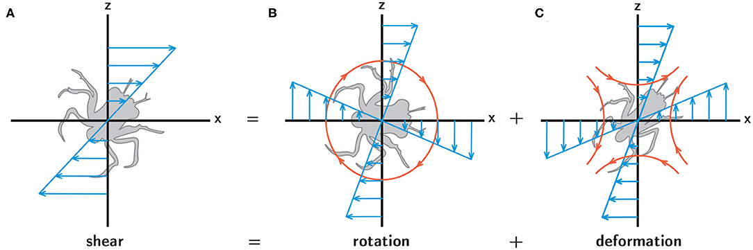
Figure 2. A simple shear flow (A) can be decomposed into fluid rotation (B) and deformation (C). In each panel the blue arrows indicate the spatial structure of the corresponding flow components, and in (B,C) the orange lines and arrows indicate the resultant rotation (B) and stretching (C) experienced by larvae.

There are two primary questions the present study seeks to answer. First, do hydrodynamic cues associated with spatiotemporally persistent flow features affect individual behavioral processes of dispersed decapod crab larvae? And second, given that regions of enhanced productivity in situ are often characterized by strong hydrographic gradients both vertically and horizontally, do differing spatial orientations of persistent hydrodynamic cues relative to gravity produce differential behavioral responses? To differentiate among spatial orientations, we use the terms “front” and “cline” generally to denote regions of enhanced spatial gradients of fluid velocity (or shear), temperature, salinity, nutrients, or other associated hydrographic variables, in which the predominant gradient (direction of most rapid change) is in the horizontal (front) and vertical (cline) directions (Woodson and McManus, 2007; McManus and Woodson, 2012; Woodson et al., 2012).

2. Materials and Methods

To investigate the relevance of spatiotemporally persistent hydrodynamic cues on larval behavior, free-swimming behavioral assays were conducted with megalopae of the common Atlantic mud crab Panopeus herbstii (Figure 3) in a laboratory flume system that uses a laminar slot jet to produce steady fluid shear layers (Figure 4A). To investigate the importance of the directional orientation of the hydrodynamic cue relative to gravity, the main test section could be rotated into three different flow configurations, corresponding to the direction of the bulk flow produced by the jet: upwelling, downwelling, and horizontal. The flow fields were quantified and tuned to produce ecologically-relevant hydrodynamic conditions for larval assays. Larval swimming kinematics were quantified and analyzed under each shear flow orientation in addition to a no-flow control condition. Flow measurements and larval swimming kinematics were observed in a 10 × 10 cm window in a 25 L experimental volume, beginning 5 cm downstream of the jet nozzle opening and centered with respect to the jet centerline (Figures 4B,C).

FIGURE 3

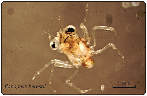
Figure 3. Megalopa of the common Atlantic mud crab Panopeus herbstii.

FIGURE 4

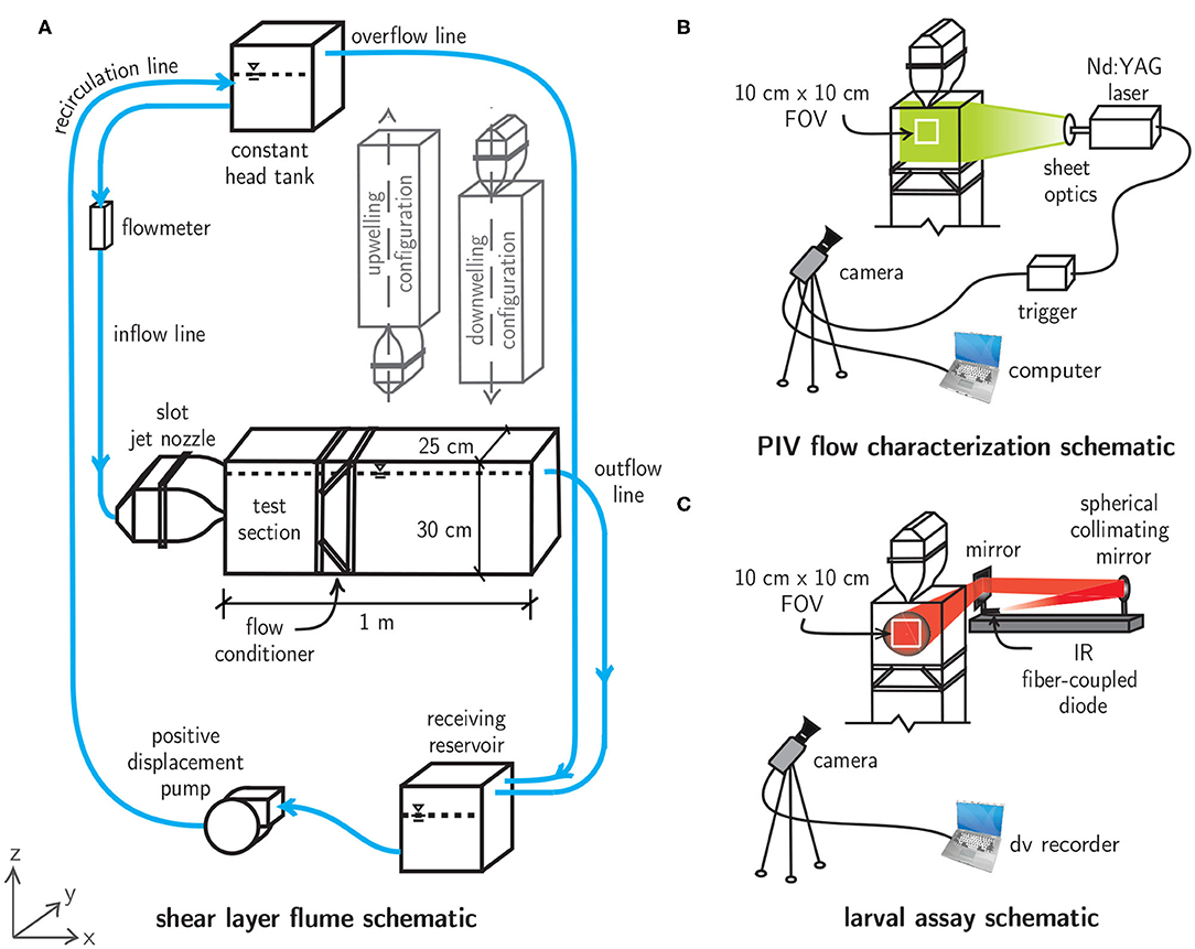
Figure 4. (A) Shear layer flume schematic featuring a main flume section that can be oriented in upwelling, downwelling, or horizontal flow configurations. The water levels in the main flume, constant head tank, and receiving reservoir are indicated by dashed lines and the free surface symbols. (B) Particle image velocimetry (PIV) schematic for flow characterization. (C) Collimated, infrared (IR) shadowgraph system for larval shear layer behavioral assays.

2.1. Shear Layer Flume

The shear layer flume is a recirculating flow system that uses a laminar slot jet (the Bickley jet) to produce steady fluid shear layers with tunable hydrodynamic characteristics. The main flume section is constructed of clear acrylic for optical access and can be rotated into upwelling, downwelling, or horizontal flow configurations (Figure 4A). An elevated constant head tank (28 L, US Plastics) with a free surface overflow drives flow with adjustable volumetric flowrate (Dwyer Instruments rotameter) through a slot jet nozzle (316 SS, jet opening 1 × 25 cm), creating a steady fluid shear layer in the main test section due to the dynamics of the laminar, planar free jet downstream of the nozzle opening. A 12:1 area ratio contraction was employed with a 5th-order polynomial contraction to prevent flow separation and to minimize turbulent fluctuations in the upstream section. Stainless steel mesh (50% open area) and a layer of high porosity polypropylene sponge inside the main body of the nozzle further dampen turbulent fluctuations and distribute fluid momentum across the width of the nozzle opening. These design features ensure a uniform (top-hat) velocity profile at the nozzle exit and produce a laminar, steady match to the analytical velocity field immediately downstream in the observation section (Bickley, 1937; Mehta and Bradshaw, 1979; Hussein, 1994; Woodson et al., 2005). The jet flow in the main test section continues through a custom flow conditioner which prevents recirculation, flow instability, and exit geometry effects. Finally, the flow continues via either a free-surface overflow or intermediate constant head reservoir (horizontal or vertical flow configurations, respectively) into a receiving reservoir (28 L, US Plastics). From there, it is pumped through a positive displacement pump (JABSCO Model 31801-1305) to the constant head tank in a closed loop.

The shear layer flume employed here, and previously (Woodson et al., 2005, 2007; True et al., 2015), is noteworthy in that it is tunable and therefore capable of matching hydrodynamic characteristics for a range of ecologically-relevant oceanographic shear flow features. This is advantageous for studying the interactions of free-swimming plankters of various species and life stages with persistent shear flow features in varying ecological contexts. Another advantageous feature is the existence of a known analytical solution for the steady shear flow produced by the laminar slot jet (Bickley, 1937), which provides a useful benchmark for assessing the steadiness and repeatability of the flow conditions produced in the apparatus. The analytical solution also provides a priori knowledge about the hydrodynamic conditions a laminar slot jet will produce under given operational parameters. Bickley (1937) considers a steady, incompressible, two-dimensional flow generated by a viscous fluid issuing from a long narrow orifice into a body of the same fluid at rest. Assuming the Prandtl boundary layer equations provide a good description of the free jet and noting that the dynamic pressure is invariant in both the streamwise (x for horizontal flows or z for vertical flows) and transverse (z for horizontal flows or x for vertical flows) directions, the flow is governed by the continuity equation,

$\begin{array}{ll}\frac{\partial u}{\partial x}+\frac{\partial w}{\partial z}=0,& (1)\end{array}$

and the streamwise momentum equation. For example, the x-momentum equation for the horizontal flow configuration (Figure 4) is

$\begin{array}{ll}u\frac{\partial u}{\partial x}+w\frac{\partial u}{\partial z}=\nu \frac{{\partial }^{2}u}{\partial z^2},& (2)\end{array}$

where u and w are the x- and z-components of velocity, respectively, and ν is the kinematic viscosity. For simplicity, the focus below is on the horizontal flow case. The flow is subject to the following three boundary conditions: symmetry about the jet centerline and boundedness in the transverse direction,

$\begin{array}{ll}\frac{\partial u}{\partial z}=0atz=0,& (3)\end{array}$

$\begin{array}{ll}w=0atz=0,& (4)\end{array}$

$\begin{array}{ll}u\to 0asz\to \pm \infty .& (5)\end{array}$

Further, the total streamwise momentum, M, is conserved such that

$\begin{array}{ll}M=\rho {\displaystyle {\int }_{-\infty }^{\infty }}{u}^{2}dz=initialstreamwisemomentumflux.& (6)\end{array}$

Following the solution method of Schlichting (1933), Sato and Sakao (1964) give the following self-similar form of the nondimensional velocity profile

$\begin{array}{ll}\frac{u}{u_o}={\text{sech}}^2\left(\frac{az}{{\delta }_j}\right),& (7)\end{array}$

where a = 0.88136. The maximum (centerline) velocity, u_o, deceases with distance downstream due to lateral entrainment of low momentum fluid as

$\begin{array}{ll}{u}_o={\left(\frac{3M^2}{32\nu x}\right)}^{1/3}& (8)\end{array}$

and the jet half-width δ_j, i.e., the transverse location at which the local velocity is half the centerline velocity at a given streamwise location, is

$\begin{array}{ll}{\delta }_j=a{\left(\frac{48{\nu }^2{x}^2}{M}\right)}^{1/3}.& (9)\end{array}$

The centerline velocity is mathematically singular at x = 0 (the physical location of the slot jet orifice), which has given rise to the idea of a virtual origin as the streamwise location of a point source of momentum a small distance upstream of the orifice from which the jet can be considered to emanate (Andrade, 1939; Sato and Sakao, 1964; Revuelta et al., 2002; Peacock et al., 2004). The virtual origin correction accounts for the non-zero nozzle width; for all shear flows here with nozzle width d_j = 1 cm and jet Reynolds number Re_j = 52, described in detail below, the virtual origin correction is not necessary to obtain a satisfactory match between the measured and predicted velocity fields. Up to jet Reynolds numbers of about 50, irregular velocity fluctuations near the orifice dampen out in the streamwise direction and the flow is steady and laminar within a few nozzle widths downstream (Sato and Sakao, 1964).

2.2. Flow Characterization

The fluid velocity and associated gradient (vorticity, shear strain rate) fields were quantified using time-resolved particle image velocimetry (PIV) for each shear flow configuration (Figure 4B). The flow was seeded with low Stokes number titanium dioxide particles (diameter 5 μm) and illuminated with a sheet of laser light from a dual-cavity, pulsed Nd:YAG laser (New Wave Research Gemini, 532 nm, 125 mJ/pulse). The laser beam was focused with a spherical lens (focal length f = 1 m) and then expanded into a thin sheet with a cylindrical lens (f = −12.6 mm), illuminating the shear layer flow in the observation window. Double-frame images were captured at 15 Hz using an eight-channel pulse generator (Berkeley Nucleonics Model 500D), which triggered synchronized laser pulses and image acquisition (CCD, Kodak Megaplus ES 1.0, 1 MP, 8-bit monochrome). The camera was equipped with a 105 mm lens (Nikon AF Micro Nikkor). Images were processed and analyzed using DaVis software (LaVision GmbH). PIV best practices (Raffel et al., 2018) were utilized to maximize measurement quality, including optimal particle seeding densities of 8-10 particles per correlation window, particle displacements of 5–10 px between successive frames (“1/4 rule”), 2–3 px particle image diameters, and multi-pass (iterative) cross-correlation schemes with overlapping subwindows (50–75 %) of decreasing sizes (64–16 px).

2.3. Larval Collection and Care

Panopeus herbstii larvae were collected from Wassaw Sound at Priest Landing (Skidaway Institute of Oceanography) on Skidaway Island near Savannah, GA, USA. Larvae were collected in late spring (end of May/early June) when planktonic (dispersed) megalopae exhibited predictable, high-density surface aggregations during nightime slack tides. A light trap was deployed from the dock between 10 pm and midnight (on slack tide). The trap consisted of a plastic jar (5 L Nalgene) with an inverted funnel designed to increase retention of larvae drawn in by a dive light secured to the bottom of the jar. The assembly was suspended horizontally between a weighted mooring device on the bed and a float on the water surface and was retrieved after a 2 h deployment. Larvae were sorted and kept in recirculating seawater, while being fed copepod nauplii (Acartia tonsa), before being transported to the Environmental Fluid Mechanics Laboratory at the Georgia Institute of Technology for shear layer behavioral assays. Larvae were kept in well-oxygenated artificial seawater (Instant Ocean) at estuarine conditions (30 ppt, 28°C) and fed copepod nauplii (A. tonsa) and brine shrimp nauplii (Artemia spp.) over the 1 week duration in which all behavioral assays were conducted. Larvae were not fed in the 24 h prior to behavioral assays.

2.4. Shear Layer Behavioral Assays

Two-hour shear layer assays were conducted between 8 p.m. and midnight under horizontal, upwelling, and downwelling flow configurations (separately). Assays were run within this time window to reduce variability in larval behavior among shear layer assays since decapod larvae exhibit variability in ontogenetic, diel, and tidally-modulated swimming behaviors, both among and within larval stages (Shanks, 1986; Jamieson and Phillips, 1988; Hobbs and Botsford, 1992; Queiroga and Blanton, 2005). Two replicates were conducted for each flow configuration, in addition to a 1-h control (no-flow). For each assay, a group of 50–60 mixed-sex, stage-specific (megalopa) larvae were introduced to the main test section and allowed to acclimate for a one-hour period prior to the experiment. During this period, the shear layer flow was started and allowed to reach steady state while larvae were aggregated away from the flow with a white fiber-optic light. At the start of the assay, the white light was turned off and free-swimming larval swimming trajectories were observed under infrared (IR) illumination via a shadowgraph system (Figure 4C). An IR fiber-coupled diode (CVI Melles Griot, 57 PNL 054/P4/S, 660 nm, 22 mW) was collimated with a spherical mirror (Edmunds Optics, NT32-845, f = 1,524 mm) and reflected off a planar mirror toward the rear of the tank. This method provided uniform illumination throughout the experimental volume and projected larval silhouettes onto a sheet of film paper on the front surface of the tank. The shadowgraph trajectories produced over the course of each two hour behavioral assay were recorded in the observation window with a CCD camera (Pulnix, 745i, 768 × 494 px) linked to a digital video recorder. Because the three-dimensional swimming trajectories are projected onto a plane with the shadowgraph system used here, all swimming kinematic and gross path parameters (discussed below) correspond to projected two dimensional trajectories (Figure 4).

For larval assays in all flow configurations, a volumetric flowrate of 16.8 cm³/s was selected to produce ecologically-relevant hydrodynamic conditions. This flowrate for the given nozzle geometry (slot width d_j = 1 cm) results in a maximum jet exit velocity, U_j, of 6.7 mm/s and a jet Reynolds number (Re_j = U_jd_j/ν) of 52, which is in a transitionally stable, laminar flow regime (Sato, 1960). The resulting velocity field is steady in time and features smooth gradients throughout the observation window. The corresponding hydrodynamic cue fields (shear strain rate and vorticity) feature large, steep gradients in the transverse direction (z for the horizontal configuration or x for the vertical configurations) and small, gradual gradients in the streamwise direction (x or z depending on the flow configuration). For all flow configurations, there are no gradients in the y-direction as a result of the slot jet used here (large aspect ratio rectangular nozzle opening), justifying the use of two-dimensional flow characterization and larval swimming kinematic analyses.

2.5. Kinematic Analysis

Raw trajectory data were digitized using LabTrack (BioRAS) software with a temporal resolution of 66.67 ms (15 Hz), sufficient to accurately resolve larval swimming kinematics. For example, larvae exhibited typical maximum relative swimming speeds up to 2 cm/s. For an image magnification of 0.2 mm/pixel and a typical larval carapace length of 2 mm, this maximum relative swimming speed results in a displacement of 10 body lengths per second, or 2/3 body length per frame. The kinematics of the resulting raw swimming trajectories (x, z, t, Figure 5) were analyzed using a suite of custom MATLAB codes to compute path kinematics including relative swimming speed [mm/s], relative swimming acceleration [mm/s²], directional heading relative to the bulk flow direction [°, ranging from 0 to 360, where 0 is aligned with the bulk flow direction], change in directional heading [°, difference in directional heading between successive displacement vectors], and turn frequency [turns/larva/s]. For relative swimming speed and acceleration, the local fluid velocity computed from the PIV data is subtracted to isolate the larval motion relative to the local flow. For turn frequency, a “turn” event is universally defined as a change in directional heading of 15° or more between successive displacement vectors.

FIGURE 5

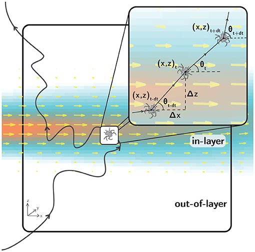
Figure 5. A hypothetical larval swimming trajectory (black line) in the observation window (large black rectangle). The fluid shear layer is denoted by the velocity vectors (yellow) and velocity magnitude contours (orange to blue). The inset (small black rectangle) shows a detailed view of kinematic parameters used to quantify swimming behavior during shear layer assays. The two-dimensional swimming trajectory projections are characterized by larval positions at each time step [x(t), z(t)] and displacement vectors of varying magnitude with directional headings θ(t) relative to the bulk flow direction.

Figure 5 shows a hypothetical larval trajectory in the 10 cm x 10 cm observation window that encompasses both in-shear layer and out-of-shear layer regions (“in-layer” and “out-of-layer,” respectively), as delineated by a threshold hydrodynamic value. For example, for a vorticity delineation (contour) of 0.2 s⁻¹ (corresponding to the light blue edge of the layer in Figure 5), the fluid shear layer occupies approximately 40% of the observation window. Segmenting the observation window into in-layer and out-of-layer regions provides a useful context for kinematic analyses comparing larval swimming behavior as a function of location relative to the shear layer (in-layer vs. out-of-layer) or historical exposure to the shear layer (pre-first-contact vs. post-first-contact). Analyzing larval swimming kinematics by location and exposure provides complementary insights into behavioral response trends associated with the spatial scale of the layer itself and short time scales (by location) as well as the relatively larger scale of the vicinity of the layer (the encompassing volume) and longer time scales (by exposure).

In addition to analyzing swimming kinematics, gross trajectory parameters were computed to examine the net effect of kinematic changes on macroscale trajectory characteristics. These include the following: net-to-gross-displacement ratio (ngdr = net displacement/gross displacement), the vertical net-to-gross-displacement ratio (vngdr = net vertical displacement/gross vertical displacement), and the proportional residence time (prt = time spent in-layer/total time in observation window). ngdr ranges from 0 to 1, with small values (→ 0) indicating more diffuse trajectories (curved, loopy), and large values (→ 1) indicating more ballistic trajectories (straight). vngdr also ranges from 0 to 1 and describes the vertical diffusivity of the swimming trajectory, and thus can be viewed as a spectrum of depth-keeping behaviors. Small vngdr values (→ 0) indicate swimming behavior that counteracts sinking or vertical advection with the flow (in vertical flows), resulting in small net vertical displacement (e.g., u-shaped or c-shaped trajectories) and hence strong depth-keeping behavior. Similarly, large vngdr values (→ 1) indicate trajectories with large net vertical displacement, and thus weak depth-keeping behavior at the scale of the observation. Displacement ratio parameters were computed consistently for 4 s periods of a given trajectory and averaged over the entire trajectory to alleviate potential dependence on the trajectory duration (Tiselius, 1992). This computation period, being long relative to the imaging period and short relative to the total trajectory duration, was found to yield displacement ratio values that were relatively insensitive to small changes in the computation period (True et al., 2015).

The swimming kinematic and gross path parameters detailed above were selected for analysis as they are well-suited to address the core questions of this study: do hydrodynamic cues associated with spatiotemporally persistent flow features affect individual behavioral processes of dispersed decapod crab larvae, and do differing cue spatial orientations relative to gravity produce differential responses? These parameters also take into account the inherent limitations of our experimental apparatus and design. For example, the analysis examines the effects of flow-induced changes in swimming kinematics when possible (e.g., subtracting local fluid velocity to analyze the relative swimming speed). However, the spatial resolution of our system (larval carapace size on the order of 10 px) prohibits a full accounting of the instantaneous effects of shear flow-induced advection and rotation, which would require resolution of the larval body orientation vector and high-resolution PIV measurements in the surrounding volume. Although advection and rotation may influence other observed trajectory parameters (turn frequency, ngdr, etc.), our analysis (see below) provides compelling evidence that the results are consistent with behavioral effects, and not flow forcing, as the primary driver.

2.6. Statistical Analysis

Statistical analyses of larval shear layer behavioral responses were performed using JMP Pro 11 (2013, SAS Institute). Path kinematic responses were investigated using a single factor, nested, repeated measures ANOVA by location (in-layer vs. out-of-layer) or exposure (pre-contact vs. post-contact). The single factor (or treatment) was the flow configuration, which has four levels: control, upwelling, downwelling, and horizontal. The repeated measures aspect of the design specifies that kinematic values by location and exposure were examined and compared for individual larva. A general linear model (GLM) was used because of the unbalanced design, whereas the nested aspect accounted for potential variability across replicates (data were pooled if replicate effects were insignificant, and the pooled error variance was used). Changes in gross path parameters were evaluated using a single factor, nested ANOVA of the arcsine-transformed data sets between control and flow (upwelling, downwelling, horizontal) values. Dunnett's control tests were used for post-hoc evaluation of differences among control and flow groups. Arcsine transformation of proportional data (gross path parameters) was required to satisfy ANOVA assumptions of normality and homoscedasticity (Zar, 1999). For some proportional data types (binomial) the logit transform is superior in satisfying linear modeling assumptions, statistical power, and reduced potential for Type I statistical error (Warton and Hui, 2011); however, in the present study there is no reason to prefer the logit over the arcsine transform since the data were proportional, but not binomial (True et al., 2015). All data sets were examined and tested for normality (Shapiro-Wilk goodness-of-fit) and homoscedasticity (examination of fit-by-residual plots for fan or funnel shapes) prior to statistical analyses, revealing no significant departures.

Significant efforts were made to reduce the possibility of pseudo-replication and to ensure statistical independence of larval swimming trajectories such that they could be treated as independent samples. For example, for all assays the number of digitized swimming trajectories was less than the number of larvae introduced to the test section in order to minimize the possibility of repeated sampling of a given larva (pseudo-replication). Larvae typically had only one sustained interaction with the shear layer and aggregated downstream at the end of the test section, both of which suggest a low likelihood of larval resampling. The potential for larva-larva interactions was also minimized to alleviate unwanted modifications to swimming behavior by using a low population density in the test section of approximately 2 larvae/L; this resulted in rare observations of more than two larvae in the observation window at any time.

3. Results

3.1. Flow Characterization

Planar PIV measurements of the flow field produced by the laminar, planar free jet in the shear layer flume are shown in Figure 6 for horizontal (Figures 6A,B), upwelling (Figures 6C,D) and downwelling (Figures 6E,F) flow configurations. In the left column, the fluid velocity (vectors) and vorticity magnitude (contours) fields show steady (time-invariant) and near-identical spatiotemporal structure among the different flow configurations, with the obvious exception of the bulk flow direction. The peak streamwise velocity along the jet centerline (u_o or w_o, depending on flow configuration) varies in the streamwise direction (x for the horizontal configuration or z for the vertical configuration, Equation 8) from approximately 6.5 to 4.5 mm/s, and the streamwise velocity (u or w, depending on flow configuration) decays smoothly in the transverse direction (z or x, depending on the flow configuration) from a peak at the centerline. Strong, steep velocity gradients in the transverse direction become gradually smoother with streamwise distance from the jet exit as lateral fluid entrainment causes gradual broadening of the velocity profile due to transverse diffusion of fluid momentum. Vorticity reaches a maximum near 0.8 s⁻¹ in two symmetric peaks off of the jet centerline that decay rapidly in the transverse direction and gradually in the streamwise direction. The vorticity peak locations correspond to the strongest velocity gradients at the edges of the jet, and there is a local vorticity minimum on the jet centerline where the transverse velocity gradient goes to zero. The steep vorticity gradients at the edges of the jet provide a well-defined demarcation of the fluid shear layer and corresponding in-layer and out-of-layer regions of the observation window (Figure 5). The gradual broadening of the velocity profile in the streamwise direction causes the layer half-width, as defined by the 0.2 s⁻¹ vorticity isocontours, to grow from approximately 10.25 to 21.25 mm over the streamwise extent of the observation window. This follows readily by taking the derivative of Equation (7) with respect to the transverse direction (z or x, depending on the flow configuration) and solving for the transverse location of the vorticity isocontour, and the half-widths so defined agree well with the measured vorticity fields (Figures 6A,C,E). Given the satisfactory agreement between the analytical and measured flow conditions, the analytical vorticity-based half-width was used to define a common in-layer region for the ANOVAs to mitigate small differences in layer definitions among different shear flow orientations (discussed more below). The shear strain rate field is not presented here, but is structurally identical to and spatially coincident with the vorticity field, with magnitude reduced by 1/2.

FIGURE 6

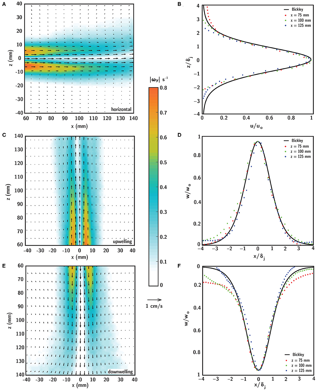
Figure 6. Time-averaged fluid velocity (black vectors) and vorticity magnitude (contours) fields in (A) horizontal, (C) upwelling, and (E) downwelling shear layers generated by a laminar, planar free jet at Re_j = 52. Comparison of analytical (Bickley) and experimental (PIV) self-similar velocity profiles extracted at various streamwise locations for the (B) horizontal, (D) upwelling, and (F) downwelling shear layers. Scaling parameters for the velocity profiles in (B,D,F) are defined in Equation (7).

In all flow configurations, the experimental (PIV) fluid velocity field agrees well with the steady analytical solution of Bickley given in Equation (7) (Bickley, 1937) as shown in the self-similar velocity profiles for each shear flow orientation in Figures 6B,D,F. Experimental transverse profiles of streamwise velocity (u or w, depending on flow configuration) taken at various streamwise locations (colored symbols) are scaled by the local jet half-width δ_j (Equation 9) and centerline velocity u_o (Equation 8) and collapse well onto the self-similar solution of Bickley (black line). Thus, there is good agreement between the analytical and experimental flow fields throughout the observation window, with negligible differences among the different flow configurations. Note that small differences in flow conditions among the different shear flow orientations, such as the more rapid decay in the transverse direction of the analytical velocity profile relative to the downwelling profile in Figure 6E, are unlikely to significantly affect results since the strong velocity gradients are well-confined to the in-layer region and both velocity magnitudes and gradients are near-zero out-of-layer. Collectively, the PIV flow characterizations confirm that all shear layer flows i. are self-consistent and repeatable, ii. are steady (time-invariant), and iii. agree well with the theoretical description, producing a steady fluid shear layer, well-defined by steep transverse gradients and smooth streamwise gradients.

The PIV results in Figure 6 were used to tune the flow system and to confirm that the shear flows presented here are ecologically-relevant for larval behavioral assays. That is, to confirm that the velocity gradients (vorticity or shear strain rate) are consistent with those that dispersed decapod larvae are likely to encounter in situ in estuarine and nearshore environments. Across a variety of estuarine systems, typical total shear (composed of steady and periodic tidal components) ranges from 0.02 to 0.1 s⁻¹ (reviewed by Whitney et al., 2012). Similarly, maximum shear values reported around nearshore thin plankton layers (e.g., in a fjord system) are on the order of 0.1 s⁻¹ (Dekshenieks et al., 2001). It is useful to note that these values of oceanographic shear are defined as the change in horizontal velocity over some vertical distance (∂u/∂z), which is closely related to, but distinct from, the fluid dynamic shear strain rate (i.e., 1/2[∂u/∂z + ∂w/∂x]) or vorticity (i.e., ∂w/∂x − ∂u/∂z). For the two-dimensional simple shear flows presented here, the ∂u/∂z term dominates the ∂w/∂x term for horizontal shear layers and vice versa for vertical layers, such that the magnitude of vorticity corresponds to the definition of oceanographic shear whereas the shear strain rate is reduced by a factor of 1/2. The maximum vorticity values achieved here approach 0.8 s⁻¹; however these values are confined to small patches symmetrically located about the jet centerline at the upstream end of the observation window, with more representative in-layer vorticity values ranging from 0.1 to 0.2 ⁻¹ (Figure 6). In this context, and considering also resolution limitations in measurements that might lead to underestimation of measured shear values in situ (e.g., Woodson et al., 2005), the velocity gradients and corresponding vorticity (or shear strain rate) values presented in laboratory shear flows are comparable to reported shear values in estuarine and nearshore environments.

3.2. Hydrodynamics and Larval Swimming Kinematics

This section seeks to answer two fundamental questions: do larvae behaviorally respond to shear layers, and if so, does the response depend on the directional orientation of the layer? These questions are addressed via a detailed look at how swimming kinematics (relative swimming acceleration and change in directional heading) vary among different flow configurations (shear flow and no-flow) and examination of corresponding differences in how larvae respond to a relevant hydrodynamic cue (fluid vorticity).

Representative larval swimming trajectories for each flow configuration are shown in Figure 7 relative to the fluid shear layer indicated by the velocity vectors (yellow) and velocity magnitude contours (orange to blue). Qualitative visual comparison of larval swimming trajectories under no-flow (Figure 7A) and shear flow (Figures 7B–D) configurations suggests a more complex spatial structure (more diffuse) in the shear flow conditions. Larval swimming trajectories in shear layers exhibit more pronounced multiscale structure, potentially reflective of more variable swimming kinematics during interaction with the layer.

FIGURE 7

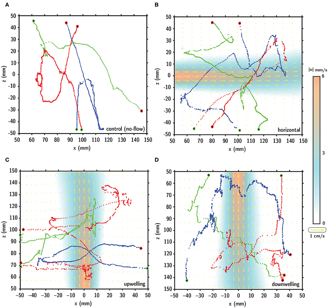
Figure 7. Digitized larval swimming trajectories in (A) no-flow (control), (B) horizontal, (C) upwelling, and (D) downwelling shear flow configurations. In (B–D), the shear layer is denoted by the velocity vectors (yellow) and velocity magnitude contours (orange to blue). In each panel, the starting and ending points of the trajectory are indicated by the green and red dots, respectively.

A more detailed view of a single larval swimming trajectory in the horizontally-oriented shear flow in Figure 8A shows a nuanced interplay between the instantaneous larval swimming behaviors and local hydrodynamic cues associated with the shear layer (Figure 8B). In Figure 8B, the orange time series is the instantaneous fluid vorticity experienced by the larva as it interacts with the fluid shear layer while progressing along its swimming trajectory. The blue curve is the corresponding instantaneous relative swimming acceleration of the larva, normalized by its maximum value. The vorticity time series clearly shows the larva entering the shear layer from below (experiencing rapidly increasing vorticity) and then exiting the layer (experiencing rapidly decreasing vorticity) before turning around, proceeding through the layer (two distinct peaks in vorticity with a local minimum between), and exiting out the top (experiencing rapidly decreasing vorticity). The acceleration time series (blue curve) shows multiple rapid corresponding changes of significant magnitude with complex temporal characteristics (rapid on/off, phase lag relative to the hydrodynamic cue, switching between acceleration and deceleration).

FIGURE 8

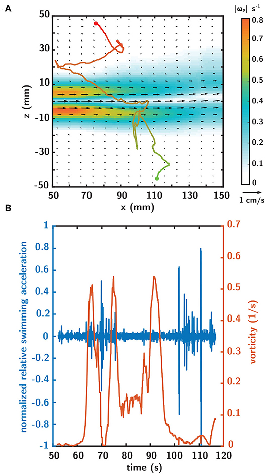
Figure 8. (A) A representative larval swimming trajectory in the horizontally-oriented shear flow as denoted by the velocity vectors (black) and vorticity magnitude contours. The starting and ending points of the trajectory are indicated by the green and red dots, respectively, and the corresponding color gradient indicates the temporal progression of the trajectory. (B) Corresponding timeseries of normalized relative swimming acceleration (blue) and fluid vorticity (orange) over the trajectory duration.

Probability density functions (pdfs) of swimming kinematics provide population-scale information about larval behavioral responses to shear flow. In Figure 9, empirical pdfs (Figures 9A,C) and corresponding cumulative distribution functions (cdfs–Figures 9B,D) of relative swimming acceleration and change in directional heading reveal marked differences among shear flow configurations. Each distribution function is a population ensemble of each timepoint for all larvae (trajectories) in a given flow configuration and each kinematic parameter was normalized within a given trajectory by that trajectory's maximum value, effectively rescaling the abscissa from −1 to 1. To improve intuition about changes in directional heading, the raw data were reoriented such that a negative value corresponds to a heading change that yields a new heading that is more against the flow whereas a positive value corresponds to one producing a new heading more aligned with the bulk flow direction. To clarify, the raw directional heading change data (i.e., the difference in successive directional heading vectors which range from 0 to 360 degrees and where 0 degrees corresponds to the bulk flow direction, Figure 5) correspond to clockwise and counterclockwise heading changes that land in the four quadrants of the Cartesian grid. The reorientation effectively compresses the data into two regions, such that one corresponds to changes in directional heading that are more aligned with the bulk flow direction (assigned to positive values) and the other more against the bulk flow direction (assigned to negative values). Since there is no flow direction for the control (no-flow) case (black curve), a hypothetical horizontal flow direction is assumed for data reorientation to ensure consistency with shear flow data reorientations; this was necessary since the raw directional heading data were also computed under this assumption, which arbitrarily assigned a directional heading of 0 degrees to the horizontal bulk flow direction for the no-flow case.

FIGURE 9

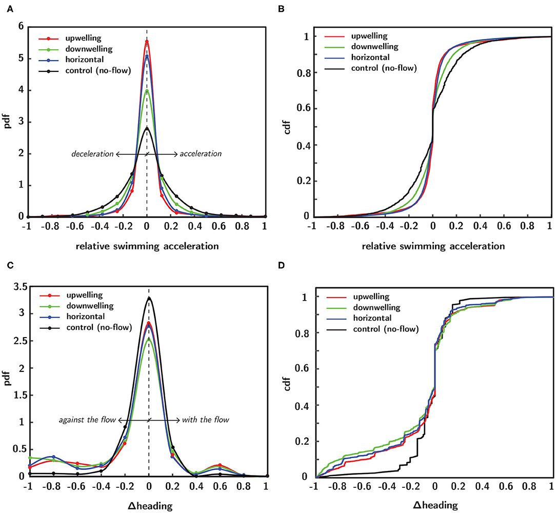
Figure 9. Empirical probability (pdf) and cumulative (cdf) distribution functions of normalized swimming kinematics in different flow configurations, including no-flow (black), upwelling (red), downwelling (green) and horizontal (blue) shear flows. Pdfs of normalized relative swimming acceleration (A) and corresponding cdfs (B). Pdfs of normalized change in directional heading (C) and corresponding cdfs (D).

Pdfs of relative swimming acceleration (Figure 9A) show that all shear flow orientations increase the kurtosis of the distributions relative to the no-flow case (black). The most significant changes were seen in the upwelling (red) and horizontal (blue) shear flow orientations, followed by downwelling (green). This compresses the values of relative swimming acceleration away from more extreme values and into a narrower band nearer to the mean. There are no clear impacts on the skewness of the distributions toward more or less acceleration relative to deceleration. The effects in the pdf are reflected in the corresponding cdfs (Figure 9B). In contrast, pdfs of heading change (Figure 9C) show that all shear flow orientations decrease the kurtosis of the distributions relative to the no-flow case (black). The most significant effects were seen in the downwelling (green) shear flow orientation, followed by horizontal (blue) and upwelling (red). This has the effect of shifting heading values away from the mean and toward more extreme values. In contrast to the relative swimming acceleration distributions, the heading change distributions do show a change in skewness associated with all shear flow orientations. The effect for all flow orientations is to shift the distributions toward heading changes that yield new directional headings that are more against the flow direction and also to focus heading changes in the flow direction into a narrower band (smaller peak). The changes are again reflected in the corresponding cdfs (Figure 9D).

To investigate corresponding differences in the hydrodynamic cue (fluid vorticity) associated with larval behavioral responses, a “consequential” behavioral response is defined as an instantaneous larval behavioral state in which both relative swimming acceleration and heading change are more than one standard deviation away from their respective mean values. In Figure 10, the statistical distributions of both the ensemble of all vorticity values encountered by larvae and the vorticity values that specifically elicit consequential behavioral responses are shown. The ensemble pdfs of all vorticity values encountered by larvae in each flow orientation are shown in Figure 10A and the corresponding cdfs in Figure 10B. The ensemble vorticity pdfs in Figure 10A resemble exponential distributions for all shear flow orientations, being weighted toward lower values but with long tails that extend to larger values. The commonality of the exponential-like distribution shapes reflect the spatiotemporal flow structure and vorticity magnitudes that larvae were exposed to in the shear flows, which are effectively identical, with the exception of the direction of the bulk flow relative to gravity (Figure 6). However, the differences in the statistical moments among different shear flow orientations (Table 1) suggest that active larval behavioral responses differ among shear flow orientations. To further explore these differences among shear flow orientations, in Figure 10C the pdfs of vorticity values that elicit consequential behavioral responses (dashed lines) are shown in addition to the ensemble vorticity pdfs from Figure 10A (solid lines). For all shear flow orientations, the consequential vorticity distributions (dashed lines) become more focused into a given vorticity range (more peaky), reminiscent of a threshold-type phenomena in which specific fluid vorticity values elicit consequential larval behavioral responses. This is reflected in the corresponding ensemble (solid lines) and consequential (dashed line) vorticity cdfs in Figure 10D. Relative to the ensemble vorticity cdfs, the consequential vorticity cdfs for all shear flow orientations are shifted upwards over a range of vorticity values, with only the downwelling shear flow showing an initial shift down at low vorticity values. The vertical shift upwards over specific vorticity ranges signifies that there is a higher cumulative probability of observing a consequential behavioral response. The differences between the consequential and ensemble vorticity cdfs (i.e. dashed minus solid lines in Figure 10D) are shown in Figure 10E. The cdf differences in Figure 10E show that the enhanced cumulative probability of a consequential behavioral response peaks at different vorticity values for each shear flow orientation. Interestingly, the vorticity peaks for all shear flow orientations correspond well with the average values of the consequential behavior vorticity pdfs (dashed lines in Figure 10C, Table 1) as signified by the stars in Figure 10E. In this light, the average fluid vorticity values that elicit consequential larval behavioral responses are good proxies for shear flow orientation-specific, threshold vorticity values. The black dashed line in Figure 10E at a vorticity of 0.2 s⁻¹ corresponds to the common vorticity value chosen to delineate in-layer vs. out-of-layer regions for ANOVAs (described in detail above), which is sufficient to encompass the enhanced cumulative probability peaks for all shear flow orientations. Thus, not only are larval behavioral responses dependent on the directional orientation of shear flows (Figure 9), but the fluid vorticity values eliciting consequential larval behavioral responses are also orientation-specific (Figure 10, Table 1).

FIGURE 10

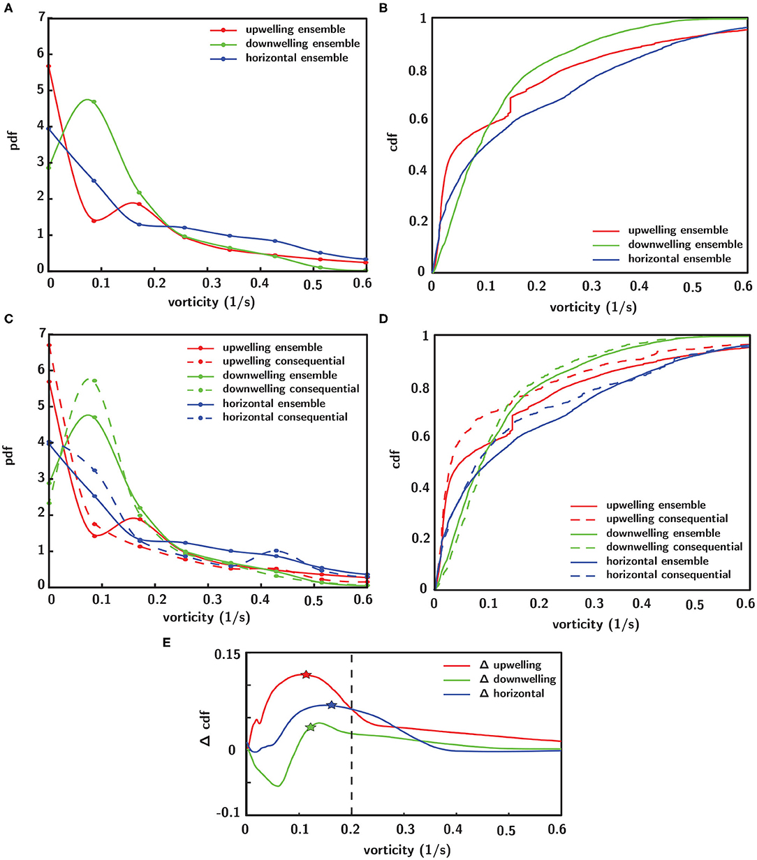
Figure 10. Empirical probability (pdf, A) and cumulative (cdf, B) distribution functions of the ensemble of all vorticity values encountered by larvae in each shear flow orientation. (C) Pdfs of fluid vorticity magnitudes eliciting consequential behavioral responses (see text for definition of “consequential”) in each shear flow orientation (dashed lines) in addition to ensemble distributions (solid lines). (D) Corresponding cdfs of consequential (dashed lines) and ensemble (solid lines) vorticity. (E) Difference in cumulative probabilities of consequential and ensemble vorticity cdfs (dashed–solid lines from D), where stars indicate the average values of the consequential behavior vorticity pdfs (dashed lines in C, Table 1) and the black dashed line at 0.2 s⁻¹ corresponds to the common vorticity value chosen to delineate in-layer vs. out-of-layer regions for the ANOVAs.

TABLE 1

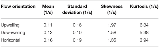
Table 1. Statistics for the probability distributions of fluid vorticity eliciting consequential larval behavioral responses in different shear flow orientations.

3.3. Larval Behavior by Shear Flow Orientation, Location, and Exposure

The evidence above suggests that larval behavioral responses to shear flow and the associated hydrodynamic cues (vorticity) for these responses depend on shear flow orientation. To evaluate potential ecological implications of these findings, the statistical significances of differences in swimming kinematics (relative swimming speed, turn frequency) and gross path parameters (ngdr, vngdr, prt) among shear flow orientations and relative to the no-flow condition are evaluated. Recall that statistical analyses of swimming kinematics are conducted by location (in-layer vs. out-of-layer) and exposure (pre-contact vs. post-contact) based on a hydrodynamic delineation of the shear layer region. The common definition used here for all layer orientations is a vorticity contour of 0.2 s⁻¹ on the outer edges of the jet, visually corresponding to the light blue edges of the layer in Figures 5, 6. This vorticity value is of the same order of magnitude as the mean vorticity eliciting consequential larval responses in all shear flow orientations (Figure 10, Table 1), but slightly larger to ensure that the defined in-layer region is readily sensed and responded to by larvae.

Relative swimming speed and turn frequency computed by location and exposure for all shear flow orientations are shown in Figure 11 and the results of the corresponding repeated measures ANOVA are summarized in Table 2. The first p-value (“Location” or “Exposure”) reports the significance of behavioral differences due to an individual larva's presence in the shear layer vs. outside of it or pre-contacting the shear layer vs. post-contact. The second p-value (“Orientation”) reports the significance of behavioral differences due to shear layer orientation (upwelling vs. downwelling vs. horizontal). Finally, the third p-value (“Location × Orientation” or “Exposure × Orientation”) is the interaction effect and evaluates whether or not behavioral differences by location or exposure are contingent upon shear layer orientation.

FIGURE 11

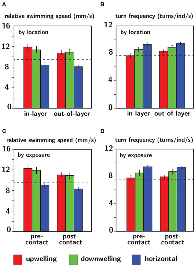
Figure 11. Relative swimming speed (A,C) and turn frequency (B,D) analyzed by location (A,B) and exposure (C,D) for upwelling (red), downwelling (green), and horizontal (blue) shear flow orientations. The dashed black lines indicate average values of each respective parameter in no-flow (control) conditions. Error bars span ± one standard error.

TABLE 2

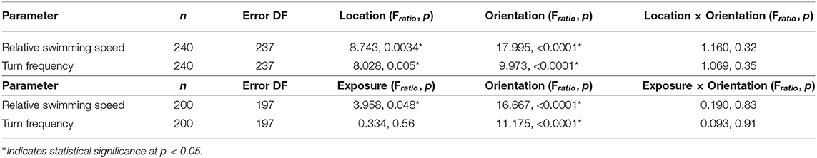
Table 2. Repeated measures analysis of variance model results for path kinematic parameters by location (in-layer vs. out-of-layer) and exposure (pre- vs. post-layer contact).

The lack of a significant interaction effect for both relative swimming speed and turn frequency signifies that differences in these parameters by location and exposure were not dependent on the orientation of the shear flow (Table 2). However, relative swimming speeds were on average significantly lower for the horizontal shear flow vs. both vertical orientations (significant orientation effect) and were slightly lower than control values (~ 9.5 mm/s). Swimming speeds in the vertical layers (~11.5 mm/s) were significantly larger. Turn frequency was on average significantly larger for the horizontal shear flow vs. both vertical orientations (significant orientation effect). Turn frequency in the horizontal shear flow (~9.25 turns/ind/s) is significantly elevated compared to control (no-flow) values (~7.5 turns/ind/s) whereas those in both vertical orientations are only slightly larger than control values (~7.75–8.25 turns/ind/s). For all shear flow orientations, relative swimming speeds were smaller post-contact (significant exposure effect) and out-of-layer (significant location effect) and turn frequency increased out-of-layer (significant location effect). Exposure and location effects in both kinematic parameters were more pronounced for the vertical shear flow orientations (orientation effects; Table 2).

Gross path parameters (ngdr, vngdr, and prt) are shown for all shear flow orientations in addition to the no-flow condition in Figure 12, and the results of the corresponding ANOVA and post-hoc Dunnett's control tests are summarized in Table 3. The first p-value reports the significance of differences in flow configuration (shear flow and no-flow) on the given gross path parameter, and the final trio of p-values indicates the significance of each shear flow orientation relative to the no-flow condition.

FIGURE 12

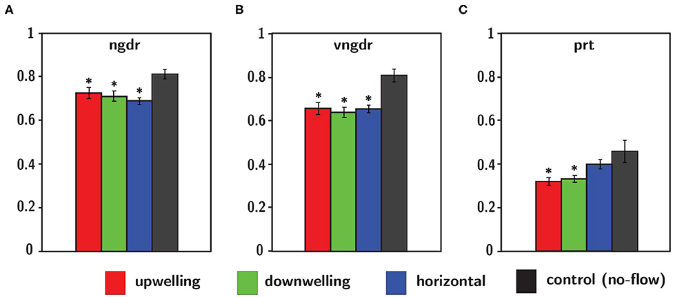
Figure 12. Gross path parameters including (A) net-to-gross-displacement ratio ngdr, (B) vertical net-to-gross-displacement ratio vngdr, and (C) proportional residence time prt for upwelling (red), downwelling (green), and horizontal (blue) shear flow orientations in addition to the no-flow condition (black). Error bars span ± one standard error. ^*Indicates statistical significance (p < 0.05) of shear flow values relative to the no-flow condition.

TABLE 3

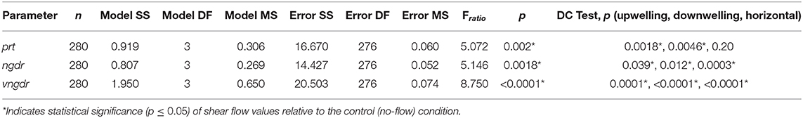
Table 3. Analysis of variance model results for gross path parameters and post-hoc Dunnett's control test results.

Reduced ngdr for all shear flow orientations (Figure 12, Table 3) is consistent with the observed increased turn frequencies, causing trajectories to become more sinuous and diffuse (i.e., smaller ngdr values). Reduced vngdr for all shear flow orientations (Figure 12, Table 3) signifies that larvae are resisting sinking and/or vertical advection through depth-keeping behaviors (i.e., smaller vngdr values). Finally, significantly reduced residence time (prt) in both vertical shear flows (Figure 12, Table 3) signifies explicit avoidance of the shear layer region, potentially as a way of resisting vertical advection for improved depth-keeping. The lack of a significant change in residence time in the horizontal shear layer indicates that the in-layer region is neither explicitly avoided nor sought out.

4. Discussion

4.1. Larval Behavior vs. Flow Forcing

It is useful to consider whether the results presented here support larval behavior or shear flow-induced forcing (advection and rotation) as the primary driver of observed swimming trajectory characteristics. Brachyuran crab larvae are some of the strongest swimmers among crustacean zooplankton and are capable of sustained swimming speeds from 0.2 to 8.3 cm/s, with typical values ranging from 0.5 to 2 cm/s (Mileikovsky, 1973; Sulkin et al., 1979; Forward, 1989a,b). Megalopae are well-equipped to sense hydrodynamic cues associated with velocity gradients through mechanosensitive setae (sensillae) distributed along appendages that are sensitive to fluid deformations and statocysts at the base of the antenna that function as accelerometers sensitive to angular accelerations induced by fluid rotation (Anger, 2001). Considering their exceptional swimming and mechanosensing capabilities relative to the weak bulk flow (6 mm/s maximum, 3 mm/s typical in-layer) and spatiotemporally persistent (predictable) vorticity structure presented in the shear layers (Figure 6), strong-swimming larvae can most likely sense and actively respond to local flow conditions everywhere without substantial shear flow-induced modifications to their swimming kinematics.

While the effects of flow-induced changes on swimming kinematics were accounted for when possible (e.g., subtracting local fluid velocity to analyze the relative swimming speed), unaccounted for advection and rotation effects may influence other observed trajectory parameters. In contrast to turbulence, with its characteristic unsteadiness and rapidly fluctuating hydrodynamic cues with differing magnitudes and spatial orientations, the flow-induced effects of steady shear flow on measured larval swimming trajectory characteristics in the present study are relatively straightforward to anticipate and evaluate. These consist of advection due to the bulk flow and rotation due to torque arising from velocity gradients (vorticity), and the anticipated effects of each on swimming kinematic parameters (relative swimming speed, turn frequency) and gross path parameters (ngdr, vngdr, prt) are discussed below. The results strongly and consistently suggest that larval behavioral processes, as opposed to flow forcing, are likely the predominant driver of observed swimming trajectory characteristics.

Comparing observed changes in swimming kinematics (relative swimming speed, turn frequency) by location (in-layer vs. out-of-layer) to expected kinematic effects of shear flow-induced advection and rotation provides a basis for evaluating the relative importance of larval behavior vs. flow forcing in observed swimming trajectories. If advective effects were significant, relative swimming speed would decrease in-layer vs. out-of-layer since the advective velocity component would dominate the active swimming velocity in the measured (raw) swimming speeds in-layer where fluid velocities are non-zero. Similarly, if rotation effects were significant, turn frequency would likely increase in-layer vs. out-of layer since a torque of sufficient strength applied to an actively swimming larva would modify the trajectory heading, increasing turn frequency in-layer relative to out-of-layer where the torque is effectively zero. The magnitude of the rotation effects will depend on the strength of the torque (vorticity) and the larva's swimming capabilities, in particular the swimming speed relative to the fluid velocity (relative swimming speed) and the ability to resist rotation (further discussion below). For both swimming kinematic parameters, the ANOVAs detected a significant location effect (in-layer vs out-of-layer) in which relative swimming speeds were higher and turn frequencies were lower in-layer (Table 2, Figure 11), opposite of what would be expected if advection and rotation effects significantly modified larvae swimming kinematics. Additionally, both kinematic parameters had significant orientation effects, but no significant interaction effects (Table 2, Figure 11). The significant orientation effect indicates that, on average, swimming kinematics depend on the spatial orientation of the shear layers, while the lack of an interaction effect indicates that in-layer vs. out-of-layer trends in swimming kinematics do not depend on layer orientation. Furthermore, the hydrodynamic conditions in shear flows of differing spatial orientation are effectively identical, with the exception of the bulk flow direction relative to gravity (Figure 6). Accordingly, the differences in overall swimming kinematics between shear flows (orientation effect) and the identical in-layer vs. out-of-layer trends (opposite of the expected shear flow-induced kinematic modifications discussed above) among different layer orientations (no interaction effect) further support the conclusion that active larval behavior, as opposed to flow forcing, is the predominant driver of observed swimming trajectory characteristics.

A similar exercise for the gross path parameters (ngdr, vngdr, prt), comparing observed changes detected in the ANOVA to expected shear flow-induced modifications to these parameters from advection and rotation, yields the same conclusion as for the swimming kinematic parameters discussed above. That is, the results strongly suggest that active larval behavior, as opposed to flow forcing, is the predominant driver of observed swimming trajectory characteristics. If advective effects were significant, swimming trajectories would become more ballistic and linear due to an additional displacement component along the parallel fluid streamlines, corresponding to an increase in ngdr (and vndgr), assuming that larvae at least resist sinking since they are negatively buoyant (Queiroga and Blanton, 2005). Similarly, if rotation effects were significant, a variety of effects could manifest in swimming trajectory ngdr (and vndgr) values, depending on the larva's swimming speed relative to the flow speed and its directional stability (i.e., ability to resist rotation) relative to the strength of the vorticity (applied torque) in the shear layer (Durham et al., 2011). Some examples spanning different regimes of rotation effects include the following: (i) pure rotations about the larva's center of mass under extremely strong torque and/or little to no directional stability, (ii) helical trajectories of varying orbital radii depending on the strength of torque and the larva's directional stability, and (iii) no significant alteration to trajectory characteristics when the torque is simply not strong enough, relative to the larva's swimming ability and directional stability, to significantly alter its directional heading. When superposed on unidirectional advection along parallel streamlines in shear flow, the first example would manifest as pure linear advection (increased ngdr) under the spatial resolution limits of our system. The second case, which was rarely, if ever, observed (e.g., Figure 7), would manifest as increasingly orbital and loopy trajectories (reduced ngdr). The results suggest that the last case is most likely, which is consistent with the swimming kinematic results and preceding discussion here. In summary, the most likely manifestation of the effects of both advection and rotation on ngdr (and vngdr) in simple shear flow would be to create more linear, ballistic trajectories, increasing the observed ngdr. The results of the ANOVA show the exact opposite: significantly reduced ngdr (and vngdr) in all shear flow orientations relative to no-flow conditions (Table 3, Figure 12). Similarly derived arguments for layer residence time (prt) would suggest that both advection (non-zero and uniform in the layer, zero out-of-layer) and rotation (non-zero in the layer, zero out-of-layer) will cause increased residence time (again assuming larvae at least resist sinking). Again, the results of the ANOVA show the exact opposite: reduced residence time in all shear flows relative to no-flow conditions (reduction in the horizontal layer is the only nonsignificant case, Table 3, Figure 12). Collectively, the results again strongly support the conclusion that active larval behavior, as opposed to flow forcing, is the predominant driver of observed swimming trajectory characteristics.

4.2. Larval Responses in Ecological Context

Considering the stage-specific ecology of decapod crab megalopae and hydrodynamic conditions in situ, what types of behaviors might one expect to observe in response to steady shear flows lacking any other environmental cue? P. herbstii inhabits estuarine waters throughout dispersal (Dittel and Epifanio, 1982) and exhibits diel, endongenous (tidal), and ontogenetic (life-stage dependent) vertical migrations (Cronin and Forward, 1979; Garrison, 1999; Miller and Morgan, 2013). Postlarval megalopae are in the dispersed larval phase directly preceding benthic settlement and they typically aggregate near the surface at night, particularly during flood tide, to enhance flood tide transport (FTT) toward favorable settlement habitats (Queiroga and Blanton, 2005). Estuarine hydrodynamics in Wassaw Sound are ideal for FTT (Forward et al., 2001, 2003b), being tidally driven (tidal range ~2–3 m) with extended periods of unidirectional flow and low wave action under normal conditions (Wilson et al., 2013). Moderate current speeds (~0.5 m/s) and relatively shallow depths (~10–15 m) yield spatiotemporally persistent, tidally-modulated vertical shear structure, while persistent horizontal shear structure is likely associated with boundary layers along the channel margins (oyster reefs, salt marsh boundaries) and complex three-dimensional circulation around weakly-stratified estuarine fronts due to relatively low freshwater input. Both fronts (elevated horizontal shear structure) and clines (elevated vertical shear structure) are typically regions of enhanced biological productivity (Largier, 1993; O'Donnell, 1993; Durham and Stocker, 2012; Woodson et al., 2012), and competent megalopae can locate and exploit these resource patches during foraging and sampling behaviors to improve fitness throughout dispersed larval stages. Thus, for imminently-settling megalopae presented with persistent hydrodynamic cues often associated with nearby resource patches, one might expect to see depth-keeping behaviors for enhanced FTT (in darkness), combined with sampling or foraging behaviors elicited by ecologically-relevant hydrodynamic cues.

Depth-regulatory behaviors are primarily driven by combined geotaxis, phototaxis, and barokinesis (Forward, 1974; Sulkin, 1975, 1984; Sulkin et al., 1980), while foraging and sampling behaviors necessarily depend on successful detection and exploitation of finescale chemical and hydrodynamic cues (Anger, 2001; Queiroga and Blanton, 2005). During the shear layer behavioral assays here, larvae experience strong rotation and deformation cues associated with steep gradients of fluid velocity along the edges of the shear layer (Figures 2, 6). As the flow is steady, effectively unidirectional, and characterized by one-dimensional velocity gradients, the local (unsteady) acceleration is identically zero and most convective acceleration terms, originating from the dot product of the velocity vector and velocity gradient tensor, are negligibly small, with the exception of those associated with in-plane shear deformation and rotation. Due to the spatial structure of the shear layers, the non-zero rotation (in-plane vorticity) and deformation (shear strain rate) cues experienced by free-swimming larvae are structurally identical and related in magnitude by a factor of two (vorticity is twice as large). Importantly, larvae are well-equipped to sense and respond to both fluid rotation and deformation. Mechanosensitive setae (sensillae) distributed along larval appendages are sensitive to fluid deformations, and statocysts as the base of the antenna function as accelerometers sensitive to angular accelerations induced by fluid rotation (Anger, 2001). While the specific hydrodynamic cue (rotation, deformation, or some combination) potentially driving larval behavioral responses to persistent shear flows is of interest ecologically (Fuchs et al., 2015; Wheeler et al., 2015), it is beyond the scope of the present study to disentangle the two. For this reason, the focus was simply on fluid rotation (vorticity) as a morphologically- and ecologically-relevant hydrodynamic cue that larvae may be responding to (Figure 10, Table 1). Clear differences in population swimming kinematics between shear flow and no-flow conditions (Figure 9) confirm that larvae readily sense and respond to the persistent rotation (vorticity) and/or deformation (shear strain rate) cues presented during shear layer behavioral assays.

What is the macro effect of larval behavioral responses to shear flows, and is it consistent with megalopal ecology? The effect of larval swimming kinematic responses to all shear flow orientations was to increase trajectory sinuosity and diffusivity (↓ ngdr) and enhance depth-keeping (↓ vngdr, ↓ prt in vertical shear layers) (Figure 12, Table 3). Increased trajectory diffusivity is consistent with observed changes in larval swimming kinematics (↓ speed post-contact and ↑ turn frequency out-of-layer, Figure 11, Table 2) and could enable larvae to remain in the vicinity of all shear layers through area-restricted search behaviors. Area-restricted searching through reduced speed and increased turning frequency is a common strategy that foraging organisms employ to locate and exploit discrete resource patches (Knell and Codling, 2012). Employing this strategy to remain in the vicinity of the shear layers, though not in the layers themselves, could provide larvae with an energetically-favorable means of simultaneously maintaining depth while also exploiting resource patches often associated with fronts and clines in situ. These behaviors would be consistent with the larval stage-specific goals of imminently-settling megalopae and suggest that hydrodynamic cues associated with spatiotemporally persistent flow features play an important, and perhaps fundamental, role in larval behavior throughout dispersal.

4.3. Orientation-Specific Responses Relative to in situ Hydrodynamics

As noted above, changes in kinematics by shear layer location and exposure were similar in all shear flow orientations (Figure 11, Table 2) and produced similar macro effects on trajectory characteristics (Figure 12, Table 3). Here, the emphasis is to highlight the significance of nuanced differences in swimming kinematics as a function of shear flow orientation, reflected in the orientation-specific kinematics pdfs and cdfs in Figure 9. The focus is specifically on why orientation-specific sensitivities to hydrodynamic cues make sense ecologically and would be advantageous to dispersed larvae.

In many relatively wide and shallow, weakly-stratified estuaries, persistent vertical shear structure (i.e., horizontally-oriented shear flows) associated with oscillating tidal flows and bottom boundary layer dynamics is characteristically stronger than persistent horizontal shear structure (i.e. vertically-oriented shear flows) around weakly-stratified estuarine fronts and along channel margins. The orientation-specific behavioral sensitivities to hydrodynamic cues (vorticity) associated with persistent shear flows seen here (Figure 10, Table 1) may be reflective of these predominant hydrodynamic realities. Larvae are most sensitive to vertically-oriented shear flows (mean consequential vorticity of 0.11–0.12 s⁻¹), suggesting an evolutionary basis for sensing and responding to typically weaker hydrodynamic cues associated with horizontal shear (vertical bulk flow) in situ. In contrast, larvae are significantly less sensitive to fluid vorticity associated with vertical shear structure (horizontal bulk flow, mean consequential vorticity of 0.16 s⁻¹), suggesting historical exposure and adaptation to more intense vertical shear structure. The higher behavioral sensitivities of larvae to hydrodynamic cues associated with horizontal shear structure may also be reflected in nuanced differences in average swimming kinematics among different shear flow orientations. For example, path kinematic responses show area-restricted search behaviors in the vicinity of all shear flows, but the response is only excited in vertically-oriented shear layers: swimming faster on average (compared to control), swimming slower post-contact and out-of-layer, and greater turn frequency out-of-layer (Figure 11, Table 2). In contrast, the area-restricted search behavior in the horizontally-oriented shear layer features slower swimming speeds on average (compared to control), swimming slower post-contact and out-of-layer, and greater turn frequency out-of-layer (Figure 11, Table 2). While all shear flow orientations elicit area-restricted search behaviors in the vicinity of the layers, the excited search behavior seen in both vertically-oriented shear layers may be reflective of larvae explicitly resisting vertical advection (↓ prt and ↓ vngdr) while also remaining in the vicinity of the layer for sampling and foraging purposes. This example highlights how orientation specificity of both behavioral sensitivity to hydrodynamic cues associated with persistent flow features and swimming kinematic responses can be advantageous for dispersed larvae. For example, they can exploit ecologically-relevant hydrodynamic cues to forage and sample for nearby resource patches (e.g., fronts and clines), while also maintaining depth to reduce predation risk or enhance tidal transport toward favorable settlement habitats.

4.4. Persistent Hydrodynamic Cues as a Potential Driver of Larval Patchiness

The area-restricted search behaviors larvae exhibit in the vicinity of all shear flow orientations offer a potential behavioral basis for finescale spatiotemporal patchiness in larval populations in situ. Observed patchiness around fronts and clines has been attributed to both physical forcing and larval behavior (Natunewicz and Epifanio, 2001). For example, Eggleston et al. (1998) found that hydrodynamic forcing significantly enhanced megalopae densities around a large-scale frontal flow feature, while Garrison (1999) attributed finescale patchiness in Brachyuran crab larva populations to interactions with small-scale hydrodynamic features. Larval responses to other environmental cues such as changing stratification and food patch dynamics in the water column were also shown to disrupt vertical migratory behaviors and produce larval patches that were depth-segregated by larval stage (Lindley et al., 1994). Collectively, it is clear that (i) planktonic decapod larva populations exhibit considerable spatiotemporal patchiness, (ii) larval patches are often found near regions of enhanced productivity and resources, including around fronts and clines, and (iii) both larval behavior and physical forcing play important roles in influencing patch dynamics. Our findings corroborate these views and quantitatively establish that hydrodynamic cues associated with spatiotemporally persistent flow features are likely fundamental drivers of decapod larval behavior and may act as a potential driver of larval patchiness by directly influencing spatiotemporal population distributions.

Area-restricted searching and increased residence time in the vicinity of persistent flow features associated with fronts and clines would offer larvae the opportunity to improve fitness by exploiting coincident high-density resources patches. Fronts (e.g., in the estuarine transition zone) and clines (e.g., in thin plankton layers) are known ecological “hot spots” in which biomass can be several orders of magnitude greater than the surrounding waters (Haury and Wiebe, 1982; Largier, 1993; O'Donnell, 1993; Yoder et al., 1994; McManus et al., 2003; Durham and Stocker, 2012). The distinct hydrodynamic signature associated with persistent flow features around fronts and clines may incentivize mechanosensitive larvae to restrict search volume in hopes of exploiting a coincident chemical cue or resource patch (a cue hierarchy, Woodson et al., 2007). The findings, highlighting the fundamental importance of hydrodynamic cues associated with persistent flow features in affecting individual larval behaviors, further suggest that fronts and clines are intimately linked to larval foraging and sampling behaviors and behavior-driven patchiness in situ (Franks, 1992; Tiselius, 1992; Epstein and Beardsley, 2001; Simons et al., 2006; Benoit-Bird et al., 2009; Woodson et al., 2012).

The need to forage and sample may also cause larvae to depart from predominant behavioral modes such as diel and endogenous (tidally-modulated) vertical migrations (Lindley et al., 1994; Woodson and McManus, 2007). Disruptions to vertical migratory behaviors have the potential to significantly influence horizontal transport and dispersal of larval populations in the context of selective tidal stream transport phenomena (Cronin and Forward, 1986; Garrison, 1999; Queiroga et al., 2002; Miller and Morgan, 2013). While there is significant variability in vertical migratory behaviors among decapod crab species and by larval stage (Sulkin, 1984), there are also many environmental cues known to modify depth-regulation and disrupt vertical migrations (i.e., light, gravity, hydrostatic pressure, turbulence). The results here show another potential source of variability in vertical-migratory behaviors in the form of enhanced depth-keeping behaviors and larval patchiness around spatiotemporally persistent hydrodynamic features. As modifiers of depth-regulation and vertical migratory behaviors, hydrodynamic cues associated with persistent flow features have the potential to significantly alter dispersal trajectories and larval population connectivity (Olmi, 1994; Marta-Almeida et al., 2006).

5. Conclusion

This study has shown conclusively that hydrodynamic cues associated with spatiotemporally persistent flow features play an important, and perhaps fundamental, role in dispersed decapod crab larval behavior. When presented with a flow feature often associated with regions of enhanced productivity around fronts and clines in situ (steady shear flow), megalopae of the Atlantic mud crab P. herbstii significantly modified swimming kinematics. Larval behavioral responses depended strongly on the directional orientation of the persistent flow feature. Furthermore, larvae exhibited orientation-specific behavioral sensitivity to a relevant hydrodynamic cue presented (vorticity), and the kinematic changes triggered in response to shear flows in all spatial orientations yielded enhanced depth-keeping and area-restricted search behaviors. These area-restricted search behaviors may be reflective of foraging and sampling initiated by an ecologically-relevant hydrodynamic cue that is potentially indicative of nearby resources patches. In this regard, hydrodynamic cues associated with spatiotemporally persistent flow features are likely fundamental drivers of decapod larval behavior and may act as another cause of larval patchiness by directly influencing spatiotemporal population distributions. This, in turn, can significantly affect larval dispersal trajectories and population connectivity in the larger ecological context of selective tidal stream transport toward favorable benthic settlement habitats.

Data Availability Statement

The datasets generated for this study are available on request to the corresponding author.

Author Contributions

AT, DW, MW, and JY conceived and designed the experiments. AT conducted the experiments and analysis. AT, DW, and MW conceived the analysis. AT and DW wrote the paper. Some aspects of this study were reported in AT's Ph.D. thesis (True, 2014). All authors approved the final manuscript.

Funding

Financial support was provided by a US National Science Foundation grant (OCE-0728238). Additional funding was provided by the Karen and John Huff Chair endowed funds.

Conflict of Interest

The authors declare that the research was conducted in the absence of any commercial or financial relationships that could be construed as a potential conflict of interest.

Acknowledgments

We thank REU researcher Allison Bergen for assistance with collection and identification of crab larvae in Wassaw Sound and digitization of larval swimming trajectories.

References

Andrade, E. C. (1939). The velocity distribution in a liquid-into-liquid jet. Part 2: The plane jet. Proc. Phys. Soc. 51, 784–793.

Google Scholar

Andrews, W. R., Targett, N. M., and Epifanio, C. E. (2001). Isolation and characterization of the metamorphic inducer of the common mud crab, Panopeus herbstii. J. Exp. Mar. Biol. Ecol. 261, 121–134. doi: 10.1016/S0022-0981(01)00268-4

PubMed Abstract | CrossRef Full Text | Google Scholar

Anger, K. (2001). The Biology of Decapod Crustacean Larvae, Vol. 14. Lisse: AA Balkema Publishers.

Google Scholar

Benoit-Bird, K. J., Cowles, T. J., and Wingard, C. E. (2009). Edge gradients provide evidence of ecological interactions in planktonic thin layers. Limnol. Oceanogr. 54, 1382–1392. doi: 10.4319/lo.2009.54.4.1382

CrossRef Full Text | Google Scholar

Bickley, W. G. (1937). The plane jet. Philos. Mag. 23, 727–731. doi: 10.1080/14786443708561847

CrossRef Full Text | Google Scholar

Criales, M. M., Zink, I. C., Haus, B. K., Wylie, J., and Browder, J. A. (2013). Effect of turbulence on the behavior of pink shrimp post larvae and implications for selective total stream transport behavior. Mar. Ecol. Prog. Ser. 477, 161–176. doi: 10.3354/meps10141

CrossRef Full Text | Google Scholar

Cronin, T. W., and Forward, R. B., Jr. (1979). Tidal vertical migration: an endogenous rhythm in estuarine crab larvae. Science 205, 1020–1022. doi: 10.1126/science.205.4410.1020

PubMed Abstract | CrossRef Full Text | Google Scholar

Cronin, T. W., and Forward, R. B., Jr. (1986). Vertical migration cycles of crab larvae and their role in larval dispersal. Bull. Mar. Sci. 39, 192–201.

Google Scholar

Dekshenieks, M. M., Donaghay, P. L., Sullivan, J. M., Rines, J. E. B., Osborn, T. R., and Twardowski, M. S. (2001). Temporal and spatial occurrence of thin phytoplankton layers in relation to physical processes. Mar. Ecol. Prog. Ser. 223, 61–71. doi: 10.3354/meps223061

CrossRef Full Text | Google Scholar

Dittel, A. I., and Epifanio, C. E. (1982). Seasonal abundance and vertical distribution of crab larvae in Delaware Bay. Estuaries 5, 197–202. doi: 10.2307/1351835

CrossRef Full Text | Google Scholar

Durham, W. M., Climent, E., and Stocker, R. (2011). Gyrotaxis in a steady vortical flow. Phys. Rev. Lett. 106:238102. doi: 10.1103/PhysRevLett.106.238102

PubMed Abstract | CrossRef Full Text | Google Scholar

Durham, W. M., and Stocker, R. (2012). Thin phytoplankton layers: characteristics, mechanisms, and consequences. Annu. Rev. Mar. Sci. 4, 177–207. doi: 10.1146/annurev-marine-120710-100957

PubMed Abstract | CrossRef Full Text | Google Scholar

Eggleston, D. B., Armstrong, D. A., Elis, W. E., and Patton, W. S. (1998). Estuarine fronts as conduits for larval transport: hydrodynamics and spatial distribution of dungeness crab postlarvae. Mar. Ecol. Prog. Ser. 164, 73–82. doi: 10.3354/meps164073

CrossRef Full Text | Google Scholar

Epstein, A. W., and Beardsley, R. C. (2001). Flow-induced aggregation of plankton at a front: a 2-d Eulerian model study. Deep Sea Res. II 48, 395–418. doi: 10.1016/S0967-0645(00)00086-2

CrossRef Full Text | Google Scholar

Forward, R. B. Jr. (1974). Negative phototaxis in crustacean larvae: possible functional significance. J. Exp. Mar. Biol. Ecol. 16, 11–17. doi: 10.1016/0022-0981(74)90069-0

CrossRef Full Text | Google Scholar

Forward, R. B. Jr. (1989a). Behavioural responses of crustacean larvae to rates of salinity change. Biol. Bull. 176, 229–238. doi: 10.2307/1541981

PubMed Abstract | CrossRef Full Text | Google Scholar

Forward, R. B. Jr. (1989b). Depth regulation of larval marine decapod crustaceans: test of an hypothesis. Mar. Biol. 176, 229–238.

Google Scholar

Forward, R. B. Jr. (1990). Responses of crustacean larvae to hydrostatic pressure: behavioral basis of high barokinesis. Mar. Behav. Physiol. 17, 223–232. doi: 10.1080/10236249009378773

CrossRef Full Text | Google Scholar

Forward, R. B. Jr., Reyns, N. B., Diaz, H., Cohen, J. H., and Eggleston, D. B. (2004). Endogenous swimming rhythms of juvenile blue crabs, Callinectes sapidus, as related to horizontal transport. J. Exp. Mar. Biol. Ecol. 229, 63–76. doi: 10.1016/j.jembe.2003.09.002

CrossRef Full Text | Google Scholar

Forward, R. B. Jr., Tankersley, R. A., and Rittschof, D. (2001). Cues for metamorphosis of brachyuran crabs: an overview. Am. Zool. 41, 1108–1122. doi: 10.1093/icb/41.5.1108

CrossRef Full Text | Google Scholar

Forward, R. B. Jr., Tankersley, R. A., Smith, K. A., and Welch, J. M. (2003a). Effects of chemical cues on orientation of blue crab, Callinectes sapidus, megalopae in flow: implications for location of nursery areas. Mar. Biol. 142, 747–756. doi: 10.1007/s00227-002-0966-7

CrossRef Full Text | Google Scholar

Forward, R. B. Jr., Tankersley, R. A., and Welch, J. M. (2003b). Selective tidal-stream transport of the blue crab Callinectes sapidus: an overview. Bull. Mar. Sci. 72, 347–365.

Google Scholar

Franks, P. J. S. (1992). Sink or swim: accumulation of biomass at fronts. Mar. Ecol. Prog. Ser. 82, 1–12. doi: 10.3354/meps082001

CrossRef Full Text | Google Scholar

Fuchs, H. L., Christman, A. J., Gerbi, G. P., Hunter, E. J., and Diez, F. J. (2015). Directional flow sensing by passively stable larvae. J. Exp. Biol. 218, 2782–2792. doi: 10.1242/jeb.125096

PubMed Abstract | CrossRef Full Text | Google Scholar

Garrison, L. P. (1999). Vertical migration behavior and larval transport in brachyuran crabs. Mar. Ecol. Prog. Ser. 176, 103–113. doi: 10.3354/meps176103

CrossRef Full Text | Google Scholar

Haury, L. R., and Wiebe, P. H. (1982). Fine-scale multi-species aggregations of oceanic zooplankton. Deep Sea Res. 29, 915–921. doi: 10.1016/0198-0149(82)90055-3

CrossRef Full Text | Google Scholar

Hobbs, R. C., and Botsford, L. W. (1992). Diel vertical migration and timing of metamorphosis of larvae of the dungeness crab Cancer magister. Mar. Biol. 112, 417–428. doi: 10.1007/BF00356287

CrossRef Full Text | Google Scholar

Houser, L. T., and Epifanio, C. E. (2009). Impacts of biochemical cues on horizontal swimming behavior of individual crab larvae. Mar. Freshw. Behav. Physiol. 42, 249–264. doi: 10.1080/10236240903165980

CrossRef Full Text | Google Scholar

Hussein, H. J. (1994). Evidence of local axisymmetry in the small scales of a turbulent planar jet. Phys. Fluids 6, 2058–2070. doi: 10.1063/1.868212

CrossRef Full Text | Google Scholar

Jamieson, G. S. and Phillips, A. C. (1988). Occurrence of Cancer spp. crab megalopae off the west coast of Vancouver Island, British Columbia. US Fish. Bull. 86, 525–542.

Knell, A. S., and Codling, E. A. (2012). Classifying area-restricted search (ars) using a partial sum approach. Theor. Ecol. 5, 325–339. doi: 10.1007/s12080-011-0130-4

CrossRef Full Text | Google Scholar

Kundu, P., Cohen, I., and Dowling, D. (2011). Fluid Mechanics, 5th Edn. Cambridge, MA: Academic Press.

Google Scholar

Largier, J. (1993). Estuarine fronts: how important are they? Estuaries 16, 1–11. doi: 10.2307/1352760

CrossRef Full Text | Google Scholar

Lecchini, D., Mills, S. C., Brie, C., Maurin, R., and Banaigs, B. (2010). Ecological determinants and sensory mechanisms in habitat selection of crustacean postlarvae. Behav. Ecol. 17, 599–607. doi: 10.1093/beheco/arq029

CrossRef Full Text | Google Scholar

Lindley, J. A., Williams, R., and Conway, D. V. P. (1994). Variability in dry weight and vertical distributions of decapod larvae in the Irish Sea and North Sea during the spring. Mar. Biol. 120, 385–395. doi: 10.1007/BF00680212

CrossRef Full Text | Google Scholar

Marta-Almeida, M., Dubert, J., Peliz, A., and Queiroga, H. (2006). Influence of vertical migration pattern on retention of crab larvae in a seasonal upwelling system. MEPS 307, 1–19. doi: 10.3354/meps307001

CrossRef Full Text | Google Scholar

McManus, M. A., Alldredge, A. L., Barnard, A. H., Boss, E., Case, J. F., Cowles, T. J., et al. (2003). Characteristics, distribution and persistence of thin layers over a 48 hour period. Mar. Ecol. Prog. Ser. 261, 1–19. doi: 10.3354/meps261001

CrossRef Full Text | Google Scholar

McManus, M. A., and Woodson, C. B. (2012). Plankton distribution and ocean dispersal. J. Exp. Biol. 215, 1008–1016. doi: 10.1242/jeb.059014

PubMed Abstract | CrossRef Full Text | Google Scholar

Mehta, R. D., and Bradshaw, P. (1979). Design rules for small low speed wind tunnels. Aeronaut. J. 83, 443–449.

Google Scholar

Mileikovsky, S. A. (1973). Speed of active movement of pelagic larvae of marine bottom invertebrates and their ability to regulate their vertical position. Mar. Biol. 23, 11–17. doi: 10.1007/BF00394107

CrossRef Full Text | Google Scholar

Miller, S. H., and Morgan, S. G. (2013). Interspecific differences in depth preference: regulation of larval transport in an upwelling system. Mar. Ecol. Prog. Ser. 476, 301–306. doi: 10.3354/meps10150

CrossRef Full Text | Google Scholar

Natunewicz, C. C., and Epifanio, C. E. (2001). Spatial and temporal scales of patches of crab larvae in coastal waters. Mar. Ecol. Prog. Ser. 212, 217–222. doi: 10.3354/meps212217

CrossRef Full Text | Google Scholar

O'Donnell, J. (1993). Surface fronts in estuaries: a review. Estuaries 16, 12–39. doi: 10.2307/1352761

CrossRef Full Text | Google Scholar

Olmi, E. J. (1994). Vertical migration of blue crab Callinectes sapidus megalopae: implications for transport in estuaries. Mar. Ecol. Prog. Ser. 113, 39–54. doi: 10.3354/meps113039

CrossRef Full Text | Google Scholar

Ott, F. S., and Forward, R. B. Jr. (1976). The effect of temperature on phototaxis and geotaxis by larvae of the crab Rhithropanopeus harrisii (gould). J. Exp. Mar. Biol. 23, 97–107. doi: 10.1016/0022-0981(76)90134-9

CrossRef Full Text | Google Scholar

Peacock, T., Bradley, E., Hertzberg, J., and Lee, Y. (2004). Forcing a planar jet flow using mems. Exp. Fluids 37, 22–28. doi: 10.1007/s00348-004-0780-8

CrossRef Full Text | Google Scholar

Queiroga, H., and Blanton, J. (2005). Interactions between behaviour and physical forcing in the control of horizontal transport of decapod crustacean larvae. Adv. Mar. Biol. 47, 107–214. doi: 10.1016/S0065-2881(04)47002-3

PubMed Abstract | CrossRef Full Text | Google Scholar

Queiroga, H., Moksnes, P., and Meireles, S. (2002). Vertical migration behaviour in the larvae of the shore crab Carcinus maenas from a microtidal system (Gullmarsfjord, Sweden). Mar. Ecol. Prog. Ser. 237, 195–207. doi: 10.3354/meps237195

CrossRef Full Text | Google Scholar

Raffel, M., Willert, C. E., Scarano, F., Kähler, C. J., Wereley, S. T., and Kompenhans, J. (2018). Particle Image Velocimetry: A Practical Guide. New York, NY: Springer.

Google Scholar

Revuelta, A., Sanchez, A. L., and Linan, A. (2002). The virtual origin as a first-order correction for the far-field description of laminar jets. Phys. Fluids 14, 1821–1824. doi: 10.1063/1.1473650

CrossRef Full Text | Google Scholar

Rodriguez, R. A., and Epifanio, C. E. (2000). Multiple cues for induction of metamorphosis in larvae of the common mud crab Panopeus herbstii. Mar. Ecol. Prog. Ser. 195, 221–229. doi: 10.3354/meps195221

CrossRef Full Text | Google Scholar

Sato, H. (1960). The stability and transition of a two-dimensional jet. J. Fluid Mech. 7, 53–80. doi: 10.1017/S0022112060000049

CrossRef Full Text | Google Scholar

Sato, H., and Sakao, F. (1964). An experimental investigation of the instability of a two-dimensional jet at low Reynolds numbers. J. Fluid Mech. 20, 337–352. doi: 10.1017/S0022112064001264

CrossRef Full Text | Google Scholar

Schlichting, H. (1933). Laminare strahlausbreitung. ZAMM 8, 260–263.

Google Scholar

Shanks, A. L. (1986). Vertical migration and cross-shelf dispersal of larval Cancer spp. and Randallia ornata (crustacea:brachyura) off the coast of southern California. Mar. Biol. 92, 189–199. doi: 10.1007/BF00392836

CrossRef Full Text | Google Scholar

Simons, R. D., Monismith, S. G., Johnson, L. E., Winkler, G., and Saucier, F. J. (2006). Zooplankton retention in the estuarine transition zone of the St. Lawrence Estuary. Limnol. Oceanogr. 51, 2621–2631. doi: 10.4319/lo.2006.51.6.2621

CrossRef Full Text | Google Scholar

Sulkin, S. D. (1975). The influence of light in the depth regulation of crab larvae. Biol. Bull. 148, 33–343. doi: 10.2307/1540551

PubMed Abstract | CrossRef Full Text | Google Scholar

Sulkin, S. D. (1984). Behavioral basis of depth regulation in the larvae of brachyuran crabs. Mar. Ecol. Prog. Ser. 15, 181–205. doi: 10.3354/meps015181

CrossRef Full Text | Google Scholar

Sulkin, S. D., Phillips, I., and van Heukelem, W. (1979). On the locomotory rhythm of brachyuran crab larvae and its significance in vertical migration. Mar. Ecol. Prog. Ser. 1, 331–335. doi: 10.3354/meps001331

CrossRef Full Text | Google Scholar

Sulkin, S. D., van Heukelem, W., Kelly, P., and van Heukelem, L. (1980). The behavioral basis of larval recruitment in the crab Callinectes sapidus Rathbun: a laboratory investigation of ontogenetic changes in geotaxis and barokinesis. Biol. Bull. 159, 402–417. doi: 10.2307/1541103

CrossRef Full Text | Google Scholar

Tankersley, R. A., McKelvey, L. M., and Forward, R. B., Jr. (1995). Responses of estuarine crab megalopae to pressure, salinity and light: implications for flood-tide transport. Mar. Biol. 122, 391–400. doi: 10.1007/BF00350871

CrossRef Full Text | Google Scholar

Tapia-Lewin, S., and Pardo, L. M. (2014). Field assessment of the predation risk - food availability trade-off in crab megalopae settlement. PLoS ONE 9:e95335. doi: 10.1371/journal.pone.0095335

PubMed Abstract | CrossRef Full Text | Google Scholar

Tiselius, P. (1992). Behavior of Acartia tonsa in patchy food environments. Limnol. Oceanogr. 37, 1640–1651. doi: 10.4319/lo.1992.37.8.1640

CrossRef Full Text | Google Scholar

True, A., Webster, D., Weissburg, M., Yen, J., and Genin, A. (2015). Patchiness and depth-keeping of copepods in response to simulated frontal flows. Mar. Ecol. Prog. Ser. 539, 65–76. doi: 10.3354/meps11472

CrossRef Full Text | Google Scholar

True, A. C. (2014). Ecological engines: finescale hydrodynamic and chemical cues, zooplankton behavior, and implications for nearshore marine ecosystems (Ph.D. thesis). Georgia Institute of Technology, Atlanta, GA, United States.

Google Scholar

Warton, D. I. and Hui, F. K. (2011). The arcsine is asinine: the analysis of proportions in ecology. Ecology 92, 3–10. doi: 10.1890/10-0340.1

PubMed Abstract | CrossRef Full Text | Google Scholar

Welch, J. M., Forward, R. B., Jr. and Howd, P. A. (1999). Behavioural responses of blue crab Callinectes sapidus larvae to turbulence: implications for selective tidal stream transport. Mar. Ecol. Prog. Ser. 179, 135–143. doi: 10.3354/meps179135

CrossRef Full Text | Google Scholar

Wheeler, J. D., Helfrich, K. R., Anderson, E. J., and Mullineaux, L. S. (2015). Isolating the hydrodynamic triggers of the dive response in eastern oyster larvae. Limnol. Oceanogr. 60, 1332–1343. doi: 10.1002/lno.10098

CrossRef Full Text | Google Scholar

Whitney, M. M., Codiga, D. L., Ullman, D. S., McManus, P. M., and Jiorle, R. (2012). Tidal cycles in stratification and shear and their relationship to gradient richardson number and eddy viscosity variations in estuaries. J. Phys. Oceanogr. 42, 1124–1133. doi: 10.1175/JPO-D-11-0172.1

CrossRef Full Text | Google Scholar

Wilson, M. L., Webster, D. R., and Weissburg, M. J. (2013). Spatial and temporal variation in the hydrodynamic landscape in intertidal salt marsh systems. Limnol. Oceanogr. 3, 156–172. doi: 10.1215/21573689-2373360

CrossRef Full Text | Google Scholar

Woodson, C. B., and McManus, M. A. (2007). Foraging behavior can influence dispersal of marine organisms. Limnol. Oceanogr. 52, 2701–2709. doi: 10.4319/lo.2007.52.6.2701

CrossRef Full Text | Google Scholar

Woodson, C. B., McManus, M. A., Tyburczy, J. A., Barth, J. A., Washburn, L., Caselle, J. E., et al. (2012). Coastal fronts set recruitment and connectivity patterns across multiple taxa. Limnol. Oceanogr. 57, 582–596. doi: 10.4319/lo.2012.57.2.0582

CrossRef Full Text | Google Scholar

Woodson, C. B., Webster, D. R., Weissburg, M. J., and Yen, J. (2005). Response of copepods to physical gradients associated with structure in the ocean. Limnol. Oceanogr. 50, 1552–1564. doi: 10.4319/lo.2005.50.5.1552

CrossRef Full Text | Google Scholar

Woodson, C. B., Webster, D. R., Weissburg, M. J., and Yen, J. (2007). Cue hierarchy and foraging in calanoid copepods: ecological implications of oceanographic structure. Mar. Ecol. Prog. Ser. 330, 163–177. doi: 10.3354/meps330163

CrossRef Full Text | Google Scholar

Yoder, J. A., Ackleson, S. G., Barber, R. T., Flament, P., and Balch, W. M. (1994). A line in the sea. Nature 371, 689–692. doi: 10.1038/371689a0

CrossRef Full Text | Google Scholar

Zar, J. H. (1999). Biostatistical Analysis, 4th Edn. Upper Saddle Hall, NJ: Prentice Hall.

Google Scholar