Eat or Sleep: Availability of Winter Prey Explains Mid-Winter and Spring Activity in an Arctic Calanus Population

1. Introduction

Calanoid copepods dominate the meso-zooplankton of Arctic seas, with Calanus spp. making up 91% of the overall biomass of copepods (Hirche and Kwasniewski, 1997). Calanus form a crucial part of marine ecosystems, particularly in the Arctic. Their high lipid content provides a rich energy source to much of the Arctic marine foodweb, through fish, ctenophores, little auks, and carnivorous or omnivorous zooplankton, and they form the key source of energy for high trophic levels in the Arctic, including birds, fish, and marine mammals (Falk-Petersen et al., 2009).

Three species of Calanus co-exist in the high Arctic: Calanus finmarchicus, the smallest of the Calanus species occurring in the Arctic, and derived from Atlantic waters; Calanus glacialis, larger than C. finmarchicus, predominately found in Arctic shelf waters; and Calanus hyperboreus, the largest of the Arctic copepods and mostly associated with deep Arctic waters (Conover, 1988). The three species are similar in that they are all lipid rich copepods (Falk-Petersen et al., 2009), but vary in their life histories. Calanus finmarchicus is considered an income breeder, relying on the initiation of the spring bloom to gain enough energy for egg production for that season. Calanus hyperboreus, however, is a capital breeder using its own energy reserves for reproduction. Calanus glacialis has a variable strategy - it is a capital breeder in sea-ice free systems, but will use ice algae as an energy source where possible and adopt an income breeding strategy (Daase et al., 2013; Renaud et al., 2018).

Calanus spp. are primarily herbivorous, relying on phytoplankton, in particular diatoms, to fuel reproduction, development, and to build up energy reserves (Falk-Petersen et al., 1990, 2009). Phytoplankton as a primary prey source present time and depth specific constraints, particularly in the Arctic. Following ice-melt and stratification, the nutrient-rich waters and a steep increase in light availability provide optimum conditions for a high magnitude, albeit short, spring bloom in phytoplankton (Falk-Petersen et al., 2009). However, this light availability is limited both spatially (to the surface waters), and temporally (to the ice-free period, although under-ice blooms have been detected in the Chukchi Sea by Arrigo et al., 2012). The consequence of this is that the phytoplankton bloom (a key food source for copepods) is limited to the well lit surface layer and mostly to late spring/early summer.

Copepods have evolved strategies to deal with these constraints. To avoid increased risk of visual predation in the surface layers they undertake Diel Vertical Migration (DVM), feeding in the surface during hours of darkness and migrating to depth during day (Ringelberg, 2010). DVM has further consequences for the ecosystem: migration actively transports carbon ingested at the surface to depth (Hansen and Visser, 2016), and also affects predator-prey interactions (Baumgartner et al., 2011).

To accommodate prolonged periods of low food abundance and high seasonality in primary production, Calanus build up large lipid reserves during the spring bloom by converting the compounds present in their algal diet into wax esters (Lee et al., 2006; Falk-Petersen et al., 2009). This lipid reserve then provides energy during the long period of low food availability. In addition, Calanus are able to enter a period of hibernation called diapause: descending to depths of hundreds of meters and reducing their metabolism to a quarter of that at the surface (Maps et al., 2014). Diapause results in both a reduction in predation risk and metabolic costs. The stage Calanus must reach before being able to enter diapause varies between species [CV for C. finmarchicus; CIV-CV for C. glacialis; CIII for C. hyperboreus, (Ji et al., 2012; Daase et al., 2013)]. On emerging from diapause, Calanus moult to the adult stage and reproduce. The timing of emergence and reproduction in spring affects the behaviors and success of Calanus in the following autumn (Varpe, 2012). It has generally been assumed that diapause is an essential stage in Calanus life history at mid to high latitudes (Hirche, 1996; Aksnes et al., 2004; Record et al., 2018) as a consequence of high seasonality in prey availability. However, scattered observations of active Calanus during the Polar Night have led to a range of expectations for overwinter Calanus behavior. Continuous activity of copepods during the winter has been observed using acoustic (Berge et al., 2009; Ludvigsen et al., 2018) and net (Grenvald et al., 2016; Daase et al., 2018) sampling methods. There is a response to low-levels of sunlight in the shallow layers (Ludvigsen et al., 2018), and a deeper migration in response to lunar cycles (Last et al., 2016). The existence of synchronized migrations [i.e., zooplankton populations migrating en masse, and therefore detectable using acoustic instruments, Cottier et al. (2006)] in mid-winter is controlled by solar altitude (a function of latitude), and modified by sea-ice (Hobbs et al., 2018). Both C. finmarchicus and C. glacialis have repeatedly been observed to be distributed throughout the water column in early January in the fjords and waters around Svalbard (Daase et al., 2014, 2018; Berge et al., 2015; Basedow et al., 2018), indicating that they either (i) ascend from overwintering depth and become active long before the onset of the spring bloom, or (ii) are advected into fjords and are found in the surface through mixing and upwelling (Krumhansl et al., 2018).

Although Calanus spp. are primarily herbivorous (Falk-Petersen et al., 2009), there are strong indications that they have flexible feeding strategies, switching to alternative prey sources when phytoplankton abundance is low (Kleppel, 1993; Ohman and Runge, 1994; Campbell et al., 2009). Alternative food sources include ciliates (Nejstgaard et al., 1997; Mayor et al., 2006), heterotrophic protists (Levinsen et al., 2000; Campbell et al., 2009), and copepod nauplii (Bonnet et al., 2004; Basedow and Tande, 2006), with consumption of these groups allowing for lipid synthesis and egg production even during periods of low phytoplankton abundance (Ohman and Runge, 1994). As the ratio of microzooplankton to phytoplankton increases, copepods show a greater preference for feeding on microzooplankton (Campbell et al., 2009). Chlorophyll levels are extremely low during the Polar Night (Błachowiak-Samołyk et al., 2014). Consequently, any heterotrophic activity is dependent on biogenic carbon remaining in the system from the previous summer (Berge et al., 2015), and there is building evidence that the microbial food web continues to be active throughout the Polar Night (Rokkan Iversen and Seuthe, 2011). Several likely Calanus prey groups have been observed during the Polar Night (Berge et al., 2015). Although chlorophyll levels remain almost undetectable, diatom cells have been found in the surface layers of Kongsfjorden (Berge et al., 2015), heterotrophic dinoflagellates and cilliates have been observed in December (Seuthe et al., 2011), and phototrophic flaegellates are present throughout the Polar Night (Vader et al., 2014).

The aim of this study was to gain a better understanding of the consequences of mid-winter activity on the fitness of Arctic Calanus populations, answering the question: Is being active during winter (either for a part or all of it) a dead end, or is this strategy sustainable given that alternative food sources may be available? We investigated whether Calanus might remain active to accommodate uncertainty in the phenology of the spring bloom, i.e., accepting lower fitness as a consequence of ensuring presence in the surface layer when the spring bloom starts. We used a decade of acoustic data collected in early winter from Kongsfjorden to characterize activity in the non-diapause depth layers (top 100 m). We then used a life history model to determine how the timing of the spring bloom and the amount of food available during winter will affect Calanus fitness given a range of winter activity scenarios. We followed two approaches in our model set-up: (i) we varied the timing of diapause entry and exit to investigate how diapause timings affect overall fitness, and (ii) we varied the timing of the spring bloom and the diapause exit date to find out whether Calanus spp. might adopt variable strategies in their diapause exit dates. Both of these experimental set-ups were explored within the context of varying amounts of winter prey availability.

2. Materials and Methods

2.1. Mooring Data

The underlying in-situ data for this study were collected in Kongsfjorden, a fjord at 79 °N on the west coast of Svalbard (Figure 1). Kongsfjorden is mostly ~200 m deep, although it extends to > 300 m in some basins (Cottier et al., 2005). Kongsfjorden does not have a pronounced sill, and as a result is influenced by inflow of both Atlantic water from the West Spitsbergen Current and Arctic water from the Coastal Current (Cottier et al., 2005; Tverberg et al., 2019). There is high inter-annual variation in the strength of the inflow of these water masses, but an Atlantic signature is common in the fjord especially during summer. The outer part of Kongsfjorden has been largely ice free since 2006 after a large intrusion of Atlantic water during the winter 2005-06 forced the system into a warmer state (Cottier et al., 2007).

FIGURE 1

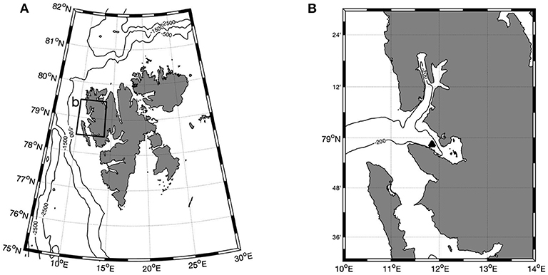
Figure 1. Location of study, Kongsfjorden, at 79 °N. (A) Kongsfjorden within the wider context of the Svalbard archipelago; (B) Detailed map of the Kongsfjorden/Krossfjorden fjord system with approximate location of mooring shown (▴). Contours of water depth are shown in m.

Calanus spp. dominate the Kongsfjorden zooplankton community in terms of biomass (Hop et al., 2019b), with both C. finmarchicus and C. glacialis co-occurring in the fjord (Kwasniewski et al., 2003). The proportion of these species varies annually as a consequence of i ) advection of Atlantic and Arctic water masses, associated with C. finmarchicus and C. glacialis populations respectively; and ii) the success of local populations within the fjord, dependent on environmental conditions (Hop et al., 2019b). The abundance of C. hyperboreus in Kongsfjorden is low, as this species is more commonly found in deep oceanic waters such as the Greenland Sea and the central Arctic Ocean (Auel and Hagen, 2002).

Temperature, fluorescence, and acoustic backscatter were measured using instruments installed on moorings in Kongsfjorden. Full details of mooring deployment times and instrument depths are provided in Table 1. Portions of this dataset have been previously described (Cottier et al., 2006; Berge et al., 2009; Wallace et al., 2010; Grenvald et al., 2016; Hop et al., 2019a).

TABLE 1

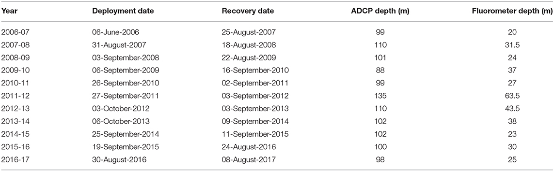
Table 1. Details of mooring deployments, including dates of deployment and recovery of the mooring platform, and depth of Acoustic Doppler Current Profiler (ADCP) and fluorometry instrumentation.

Backscatter data were collected using 300 kHz RDI Acoustic Doppler Current Profilers (ADCPs) installed in an upwards looking configuration at a nominal depth of 100 m (Table 1). Whilst backscatter from ADCPs is not calibrated for the calculation of zooplankton biomass, nor does its single frequency capacity allow for size discrimination of the acoustic targets, we were able to use our current understanding of the local zooplankton community to assess likely species within the migrating population that are represented in the ADCP data. In the autumn, Calanus have been shown to contribute up to 90% of the scattering signal as detected by ADCPs in Kongsfjorden (Berge et al., 2014). As Calanus are seen to be active during this period, and they are known to be prolific diel migrators, we are confident that the Calanus population makes up at least a significant portion of the migrating scattering signal.

The ADCP was set to sample using 4 m depth bins, and to record a series of 60 acoustic pings over a 20 s period every 20 min. These series of pings were averaged to give a single data point. The ADCPs have a sampling range of 120 m. The top few meters (typically 10 m) of each recording were deleted due to interference caused by the air-sea interface (after visual inspection of data). Acoustic backscatter data were converted to Mean Volume Backscatter Strength (S_v, dB) using the sound equation of Deines (1999). Backscatter data were normalized so that the mean of each dataset was the same (as per Wallace et al., 2010) to allow greater comparability of the variation in backscatter between datasets (although absolute backscatter between deployments is not comparable).

To derive a proxy for the DVM intensity from the acoustic backscatter data, we calculated the Lomb-Scargle power spectral density, which is a quantification of the rhythmicity (Berge et al., 2009) in the zooplankton population observed using acoustics. Data were sub-sampled using a 10-day moving window. Rhythmicity was tested for at periods in the 1 ± 0.2 day range, at 0.005 day resolution. The maximum power spectral density for this range was used as a measure of the synchronicity in the zooplankton population during each 10 day period.

Temperature data were measured through the water column using a combination of Seabird SBE 37 (Microcat), SBE 16+, SBE 56, and temperature miniloggers. Precise instrument depths varied between years, but in all years instruments monitored the majority of the water column (Cottier et al., 2005). Annual time series of water temperature were created using averaged data from all instruments available at <50 m and > 150 m to represent surface and deep temperature conditions (Figures 2A,B). These data were used to construct semi-idealized temperature time series representing average conditions during the 10 years.

FIGURE 2

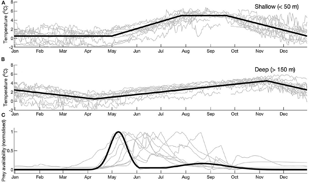
Figure 2. Time series from 10 years of mooring measurements for (A) shallow (<50 m) temperature; (B) deep (>150 m) temperature; (C) normalized fluorometry. Time series representing the full 10 years are plotted in bold lines. In (A,B), these time series are based on the averages of all 10 years. This was not possible for fluorometry (C) due to large inter-annual variability. Instead, an idealized model forcing has been created based on 1 year (2006), and inter-annual variability is captured by varying the timing of the spring bloom.

Fluorometers were installed on the moorings as auxiliary sensors to the Seabird 16+ CTD instruments. Deployment depth varied (Table 1), but fluorometers were always installed with the intention of sampling in the vicinity of the sub-surface chlorophyll maximum. The fluorometers recorded at hourly intervals. As calibrations were not conducted in some years, and fouling during long deployments can lead to sensor drift (Hop et al., 2019a), data were normalized to a 0 to 1 scale [as per Wallace et al. (2010)]. Several contributing factors meant that a time series representing the full 10 years was not possible to construct: there was large inter-annual variability in bloom phenology; uncertainty in the magnitude (as explained above); and the instrument deployment depth varied (Table 1). Therefore, an idealized curve was made based on the shape of the general fluorometry signature in Kongsfjorden (Figure 2C). The magnitude was set using data sampled in 2006: uniquely in this year, a water sample was taken during the peak of the spring bloom (Hegseth and Tverberg, 2013). Full details of chlorophyll sampling and analysis are provided in Hegseth and Tverberg (2013). For comparison with potential winter prey fields, we used a carbon:chlorophyll ratio sampled in Kongsfjorden (Clara Hoppe, pers comm.) to convert chlorophyll data (from the fluorometer) to carbon. Data were collected during the spring bloom in 2016 (27-April to 19-May) from 10 m depth. The average ratio (73.9) was used here. The carbon:chlorophyll ratio varies seasonally, and so we used data sampled during the spring bloom to correspond with the chlorophyll sample used to calibrate the magnitude of the fluorometry data.

2.2. Coltrane Model

Viable Calanus life-history strategies were investigated using a copepod life history model: Coltrane (Copepod Life-history Traits and Adaptation to New Environments) version 1.0, as described in detail by Banas et al. (2016). Matlab source code is available at http://github.com/neilbanas/coltrane.

Coltrane is an individual based model. It does not predict absolute abundance nor biomass of a population, but can be used to determine optimal life history strategies in a range of environments, which are specified using an annual prey cycle (P, measured here in μg C L⁻¹) and water temperature. The prey cycle is varied using two parameters: P_win sets the minimum amount of prey available throughout the year (and, consequently, the amount of winter prey availability), and t_max sets the timing of the peak in the spring bloom biomass.

Coltrane uses four state variables to describe a single cohort of copepods (copepods in a single cohort are spawned on the same day and have the same traits): relative developmental stage D (0 ≥ D ≤ 1, 0 at spawning, 1 at adulthood); survivorship N (the fraction of initially spawned individuals that remain, initially set to 1 and decreases with time according to predation mortality - a function of size, a temperature dependent growth rate, and a mortality coefficient); structural biomass per individual S; and individual reserve or storage-lipid biomass R. Adult body size (Wa) is the sum of R and S. The division of total body size into R and S can also be thought of as a distinction between “reversible” and “irreversible” gains of carbon and energy respectively.

Copepods develop through 13 distinct life stages [an embryonic period; six naupliiar stages (N1-6); five copepodite stages (C1-5); adulthood], defined by D in the model. The progression of D is set according to a developmental rate, u_o [set at 0.07 d⁻¹, following Banas and Campbell, 2016]; activity (a binary switch for whether copepods are in diapause or not); prey-saturation, σ, a simple Michaelis-Menten function with half-saturation, K_s, of prey availability (θ = P/(K_s+P)), where K_s is 73.9μgCL⁻¹ [equivalent to the 1μgchlL⁻¹ used in Banas et al. (2016)] and P is the prey availability as previously described); and a temperature-dependent factor (shallow (<50 m) when active, and deep (>150 m) when in diapause), as per Figures 2A,B.

The growth of copepods is defined using energy intake (when incoming energy is above the value of metabolic loss), and is allocated to both structural biomass (S, growth and structure) and reserve biomass (R, lipids and egg potential), although the allocation varies between life stages. At D < 0.35 (naupliiar stages), energy is allocated completely to structural reserves. Once copepods reach adulthood (D = 1), all energy intake is allocated to reserve biomass. Between these stages, energy is committed to a combination of the two.

Diapause is implemented in the model as a reduction in metabolism, to a 1/4 of that of active metabolic rates [as per Maps et al. (2014)]. Development and ingestion remain at zero during the enforced diapause period. Diapause is forced through the model set up, using parameters of $t_{dia}^{enter}$ and $t_{dia}^{exit}$ for the diapause entry and exit date respectively, allowing us to run permutations of diapause conditions to investigate the effect of timing (and, consequently, duration) on resultant fitness (here defined as lifetime egg production per recruited adult; Renaud et al., 2018).

The first date at which individuals can spawn eggs is set by t_egg [given that maturity has already been reached (D = 1)]. Model experiments were run for all cases of t_egg from day 0 to day 730 (2 year period) at 10 day intervals. The t_egg case with the highest fitness was then selected to represent that model run. If more than one value of t_egg resulted in equal maximum fitness, the first occurrence of max(t_egg) was used.

Figure 3 shows the state variables (D, R, S) for a model run for selected likely forcings (P_win = 20 μgCL⁻¹; t_max= 10-May; $t_{dia}^{enter}$ = 02-October; $t_{dia}^{exit}$ = 01-January) as an example of how the copepods develop within the model framework. Copepods are spawned at 5 day intervals along the y-axis, and 2 years of the model run spans out along the x-axis. White spaces show either where copepods were not yet spawned (i.e., top left of figure), or where cohorts were terminated by starvation (for spawning times in August). Black lines outline dates of diapause, as enforced by $t_{dia}^{enter}$ and $t_{dia}^{exit}$.

FIGURE 3

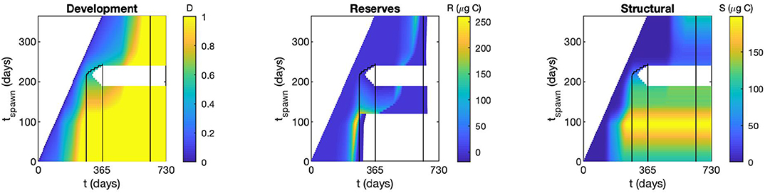
Figure 3. State variables [Development (0 at egg, 1 at adult), Reserve biomass (μgC), Structural biomass (μgC)] for a selected model run chosen to be representative of a likely scenario in Kongsfjorden. Black contours show the period within which copepods are in diapause for this example run, and white areas show non-surviving copepods.

As a consistency check on parameter choices, we compared output of the Coltrane model with Calanus collected using nets (Figure 4). Calanus were sampled with either a Hydrobios Multinet or WP2 net (mouth opening 0.25 m², mesh size 180–200 μm) from the central basin of Kongsfjorden between 2001 and 2016 (May, July-September). 961 adult females (of both C. finmarchicus and C. glacialis) were collected and prosome length was measured from the tip of the cephalosome to the distal lateral end of the last thoracic segment, and was either measured from formalin preserved Calanus using a stereomicroscope, or from digital images of live individuals as described in Daase et al. (2018). C. hyperboreus females were not included.

FIGURE 4

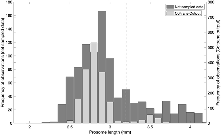
Figure 4. Comparison of predicted body size from the Coltrane model [converted from weight following Runge et al. (2006)] with net sampled Calanus from Svalbard. Dashed line at prosome length = 3.2 mm indicates separation between C. finmarchicus and C. glacialis adult females as per Kwasniewski et al. (2003).

The Coltrane output variable of adult body size (Wa, μgC) was converted to prosome length (PL) for comparison with the net data using the equation $PL=e^{\frac{log(Wa)-1.48}{3.57}}$ adapted from Runge et al. (2006).

The Length frequency distribution of adult Calanus sampled in Kongsfjorden overlaps with the length frequency distribution of adult body size as predicted by the Coltrane model (Figure 4). All of the model-predicted copepod prosome lengths fall within the expected range of Calanus in this region.

2.3. Experimental Set-Up

Two types of experiments were run, each investigating a different aspect of copepod life history: Diapause Timing Experiments (DTE) and Spring Bloom Variability Experiments (SBVE). The experimental setup of each of these cases is illustrated in Figure 5. In both experiments, the winter prey availability, P_win, was varied between 0 and 40 μgCL⁻¹ at 10 μgCL⁻¹ increments, implemented by P = max[P, P_win].

FIGURE 5

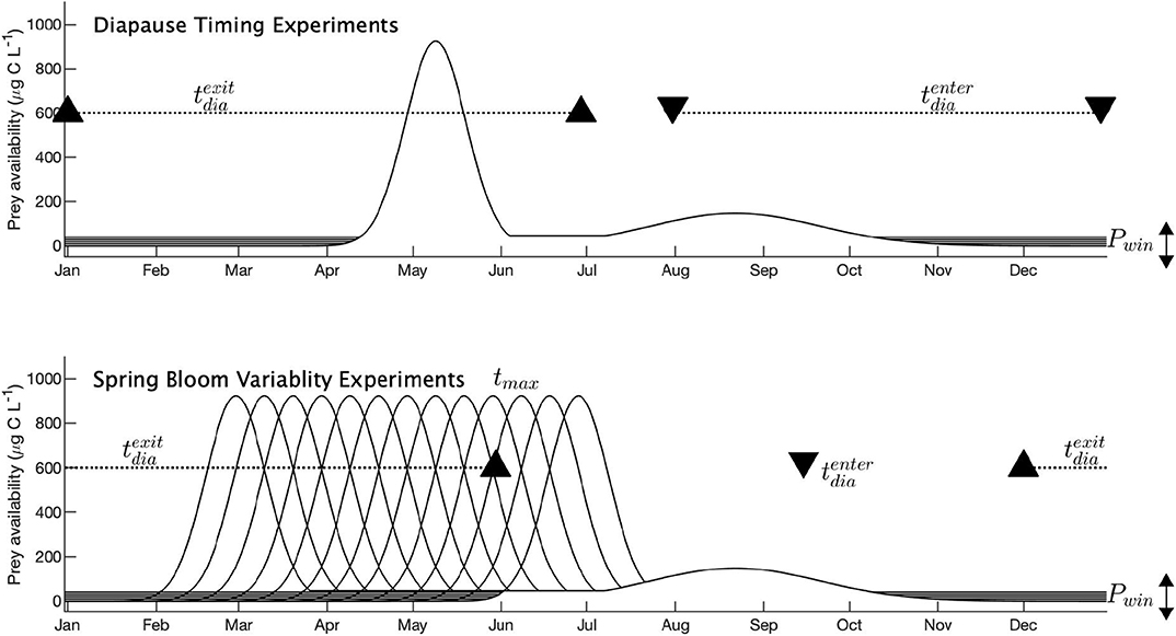
Figure 5. Experimental setup of the Coltrane model for two experiments: Diapause Timing Experiments and Spring Bloom Variability Experiments. Black solid lines indicate prey availability. Black triangles and dashed lines show diapause conditions: black triangles indicate the date of diapause entry ($t_{dia}^{enter}$, downward triangles) and diapause exit ($t_{dia}^{exit}$, upward triangles). Dashed lines show the variation allowed with some parameter values. No dashed line indicates a fixed date.

In the DTE, the timing of the spring bloom, t_max, remained constant at yearday 130 (10-May). Diapause entry dates, $t_{dia}^{enter}$, ranged from yearday 213 to 363 (n = 16), and diapause exit dates, $t_{dia}^{exit}$, ranged from 1 to 181 (n = 19), both at 10-day increments.

In the SBVE, t_max varied from yearday 60 to 180 at 10-day increments (n = 13), but the functional form remained the same. $t_{dia}^{enter}$ remained fixed at yearday 259 (15-September), and $t_{dia}^{exit}$ ranged from 336 to 150 at 10-day increments (n = 19).

3. Results

3.1. Mooring Data

Backscatter data from ADCPs were used to observe daily zooplankton migrations (Figure 6). In most years, backscatter was high during winter and early spring indicating a high abundance of migrating zooplankton, suggesting that (at least some) Calanus were out of diapause and active within the water column. Rhythmicity (as defined using the power spectral density) was highest in the period centered on 21-March each year, the Spring Equinox. Periods of strong, synchronized migration occurred for a 2 month period around this time. This period of intense, synchronized migration occurred each year before the spring bloom had started (as detected at the depth of the fluorometers, at least; Table 1), and before any sign of the initiation of a spring bloom (top panel of each year in Figure 6). High synchronicity was seen at all depths at some point during the study period, suggesting that zooplankton are migrating daily throughout the top 100 m. In some years (2007, 2009, 2015), periods of high synchronicity occur at the start of January, indicating synchronized mid-winter migrations.

FIGURE 6

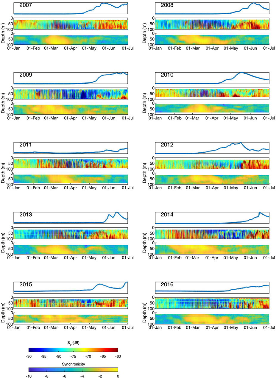
Figure 6. Fluorescence and zooplankton dynamics in Kongsfjorden, January-June in the years 2007–2016. Each year comprises three plots showing data for (from top to bottom): normalized chl-a fluorescence; ADCP backscatter (S_v, dB); synchronicity (log scale of power spectral density).

3.2. Diapause Timing Experiments

The DTE were run for a range of $t_{dia}^{enter}$ and $t_{dia}^{exit}$ (and therefore diapause duration varying from 1 to 333 days), with t_max remaining constant at 10-May. The fitness consequences for each $t_{dia}^{enter}$ and $t_{dia}^{exit}$ combination are shown in Figure 7. White regions of each plot show model runs (and therefore copepod strategies) that did not result in a viable copepod (i.e., reached starvation before maturity). At $P_{win}=0\mu gC{L}^{-1}$, viable strategies are only seen when individuals enter diapause between October and December, and exit between February and May. Exiting diapause after the spring bloom is not viable due to missing the period of high prey availability. The strategy associated with the highest fitness is a diapause entry in September, and exiting just before the spring bloom (April). As the value of P_win increases, the range of viable strategies becomes broader. Entering diapause in August is not a viable strategy except in the case of $P_{win}=40\mu gC{L}^{-1}$. The fitness consequences of short diapause or continuous mid-winter activity can be seen in the top left of each of the plots in Figure 7. By $P_{win}=20\mu gC{L}^{-1}$, this region is a viable strategy in terms of fitness. At $P_{win}=40\mu gC{L}^{-1}$, this region of short or non-existent diapause is appearing as a secondary region of high fitness (in addition to the continued area of high fitness associated with September entry and exit just before the spring bloom). As P_win increases, copepods are also able to survive when exiting diapause after the date of the peak in spring bloom biomass occurs (indicated in regions to the right of the dotted line in cases of $P_{win}\ge 20\mu gC{L}^{-1}$), but values of lifetime egg production suggest that these individuals would not be successful in terms of long term reproductive traits.

FIGURE 7

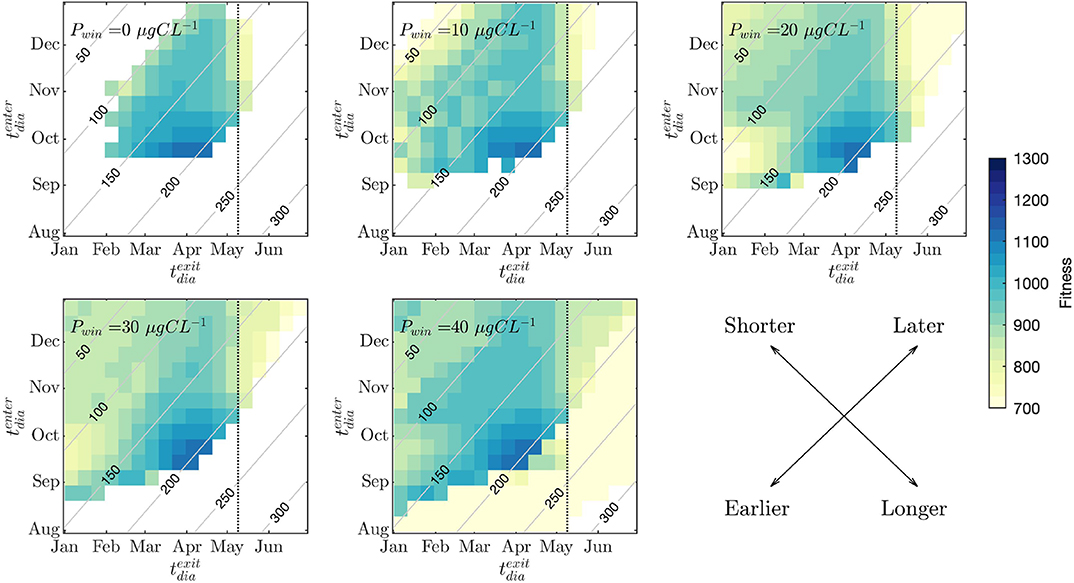
Figure 7. Diapause timing experiments. Individual plots show model experiments for each value of minimum prey availability (P_win). Fitness outcomes of each combination of diapause entry date ($t_{dia}^{enter}$) and diapause exit date ($t_{dia}^{exit}$) timing are shown in color. The date of the spring bloom maximum (10-May) is plotted using a dotted line. Gray contours show diapause duration in days. The bottom right plot shows a schematic for interpreting the results. Shorter and longer refer to diapause durations, and earlier and later to ($t_{dia}^{enter}$) and ($t_{dia}^{exit}$) .

3.3. Spring Bloom Variability Experiments

The SBVE were run for a range of t_max and $t_{dia}^{exit}$ (Figure 8). $t_{dia}^{enter}$ was fixed at 15-September across all experiments. In general, exiting diapause 1–2 months before the peak of the spring bloom (i.e., just as the spring bloom starts) is the best strategy. The range of $t_{dia}^{exit}$ that are viable do not change considerably over the various levels of P_win, remaining at December-March depending on t_max. However, as P_win increases, the range of possible t_max that can sustain successful populations increases.

FIGURE 8

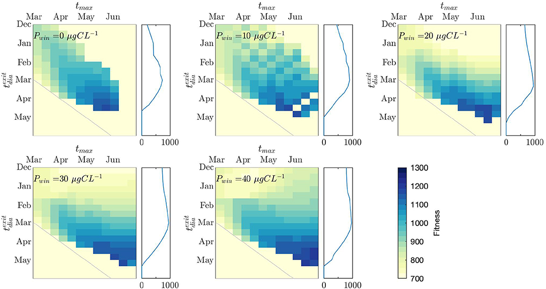
Figure 8. Spring Bloom Variability Experiments. Individual plots show experiment runs for each value of P_win. Fitness outcomes of each combination of diapause exit date ($t_{dia}^{exit}$) and the date of the spring bloom maximum (t_max) are shown in color. The gray line indicates a 1:1 date line (i.e., exiting diapause on the same day as the spring bloom peak, $t_{dia}^{exit}$ = t_max. Lower left of this line is the fitness consequence of $t_{dia}^{exit}$ occurring after t_max, upper right is the consequence of $t_{dia}^{exit}$ occurring before t_max). On the right hand side of each plot, the mean fitness consequence of each row (i.e., the mean fitness for each $t_{dia}^{exit}$ across all cases of t_max) is plotted.

The mean fitness potential for each strategy (i.e., the mean fitness across all cases of t_max for each $t_{dia}^{exit}$) can be seen in the panel to the right of each model output plot. At P_win = 0 μgCL⁻¹ there is a clear fitness advantage to exiting diapause in March (given a range of spring bloom conditions that we assume copepods cannot predict). However, as P_win increases, this fitness advantage reduces. At P_win = 20 and 30 μgCL⁻¹, there is a negligible disadvantage to exiting diapause in January. By P_win = 40 μgCL⁻¹, the difference in fitness between exiting diapause at any time between December and March is very low.

4. Discussion

We have used observational data to parameterize a life history model to explain observations of mid-winter activity in an Arctic zooplankton population in the Polar Night, and to understand the range of possible strategies that lead to successful reproduction. A key part of this investigation was to understand how life strategies are modified in response to varying winter nutrition. We found that small changes (10 μgCL⁻¹) of P_win had a large impact on the range of viable life history strategies in Calanus spp. Life strategies that involve continuous activity through the winter are found in the upper left part of each plot in Figure 7. As P_win increases, the fitness in that region increases from 0 (not viable) at 0 μgCL⁻¹ to 900 (viable) at 40 μgCL⁻¹. In each P_win scenario, the conventional diapause strategy (i.e., diapause entry in autumn and exit in spring) is optimal in terms of fitness, but the results presented here suggest that remaining active for a part, or all of winter, is a secondary strategy with comparable levels of fitness, when there is a non-zero level of winter prey availability. A key finding here is that overall Calanus fitness does not improve in scenarios of increasing winter prey, but there are increases in the range of strategies that are viable.

The values for winter prey availability were not based on definitive sampled values. The reason for this is three-fold: First, feeding experiments on copepods are rare, and so it is difficult to obtain a complete summary of likely prey sources, and how these might be ingested in terms of preference by copepods. Ciliates, for example, are underestimated in the diet of copepods when using sequencing to measure ingested prey composition, as signatures from potential parasites have to be removed from the signal, of which there is an overlap with ciliates that would be consumed as prey (Cleary et al., 2017). Second, winter studies regarding the abundance of likely prey sources have been infrequent across the Arctic. In the lead up to the spring bloom (March), a relatively high proportion of chaetognaths have been observed in the gut contents of C. glacialis (Cleary et al., 2017). Chaetognaths are primarily predators of Calanus, but it is suggested that at this time of year, Calanus will predate upon eggs and juvenile stages of chaetognaths. Sampling for abundances of these early life stages of chaetognaths has not been undertaken during the winter, and so it is not possible to quantify their potential as a winter food source in carbon terms. Calanus have also been observed to feed on copepod eggs and nauplii (Bonnet et al., 2004; Basedow and Tande, 2006). Calanus nauplii are not abundant in winter, reducing the potential for cannibalism, but a high abundance of copepod nauplii of smaller copepods (Oithona similis, Microcalanus spp.) have been observed in Svalbard fjords during the Polar Night (Grenvald et al., 2016, Berchenko pers. comm.) that could be a so far underestimated food source for Calanus. Third, the values of P_win are only meaningful relative to the value assumed for half-saturation, here defined as 73.9 μgCL⁻¹ [as per Banas et al. (2016)]. Half-saturation varies across Calanus studies, and within individual studies it varies with prey type. The P_win values used within this study were conservative, ranging from c. 0–4% of the spring bloom carbon availability, and were designed as a basis for the types of behaviors we would expect to see in Calanus given a range of winter prey availability scenarios. Because we do not have exact values of winter prey available, instead we examined winter prey availability values that explained the behaviors that have been observed in Kongsfjorden to be viable within the model framework. Following this, we expect Calanus to have a consistent availability of prey exceeding 20 μgCL⁻¹.

The timing of the spring bloom in Kongsfjorden was highly variable (Figure 2 and Hegseth et al., 2019). To account for this, we varied the date of the spring bloom in 10 day intervals from yearday 60 to 180 (01-March to 29-June) in the SBVE (Figure 8) to incorporate all scenarios from recent years (Figure 6), and to allow for earlier spring bloom conditions as predicted in a warming Arctic (Kahru et al., 2011). In general, the model output suggests that the optimal time to exit diapause is about 1 month before the spring bloom, although for any spring bloom date, exiting diapause at any time up to 2 months before the spring bloom peak is about equal in terms of fitness. The average fitness across all spring bloom dates for each diapause exit date can be used to look at optimal diapause exit timing strategies in copepods (right-hand panels in Figure 8). At low values of P_win (0 μgCL⁻¹), there is a gradient in the fitness from January through to March, with relatively low fitness in January, and the highest fitness in March. As the P_win increases, the gradient of increasing fitness as spring develops reduces. At 40 μgCL⁻¹, the fitness is almost completely consistent from January to March. As long as a small amount of prey is available throughout the winter, exiting diapause before the spring bloom does not provide an energetic disadvantage, and there is no fitness advantage in staying in diapause until the spring bloom begins. If there is no difference in fitness between exiting diapause early or remaining in diapause until the onset of the spring bloom, there may be an adaptive advantage to exit diapause early and be ready for when the spring bloom starts, instead of risking to emerge too late. Such a strategy makes sense in an environment like the seasonally ice covered Arctic shelf seas where the onset of the ice algae and phytoplankton blooms is highly variable between years. Similarly, C. glacialis populations across the Arctic show high plasticity in their reproductive strategies, relying on both income and capital breeding which has been regarded as an adaptation to deal with high variability in the spring bloom phenology (Daase et al., 2013).

Calanus populations of various life stages have repeatedly been observed to be active in January, not only in Kongsfjorden but also in other Svalbard fjords and in the oceanic waters west and north of Svalbard (Daase et al., 2014, 2018; Basedow et al., 2018). The model results presented here show that this behavior is energetically sustainable as long as alternative food sources are available. Winter studies of zooplankton populations are still rare across the Arctic, thus it is uncertain in how far the early emergence of Calanus from diapause is more widely applicable across the Arctic. Data on the vertical distribution of C. glacialis during autumn and winter from the Canadian Arctic (Daase et al., 2013; Darnis and Fortier, 2014) indicate that these populations emerge from diapause later in the winter compared to observations of Calanus in Svalbard waters (Daase et al., 2014, 2018; Basedow et al., 2018). It is unclear why these populations act differently, but our model results indicate that they may be explained by small changes in the winter prey availability. This highlights the need for further study into winter plankton ecology in Arctic waters. Furthermore, the Canadian population descends to diapause depth later in autumn than the Svalbard population (Daase et al., 2013) and the overwintering population in Amundsen Bay was characterized by a high proportion of CIII, indicating that life history strategies differ in more than one way between these populations.

Whilst acoustic observations enable year-round high resolution sampling which can not be replicated with net data, we recognize that this application of acoustic data represents population level activity rather than that of individuals. Whilst many studies using net data support the hypothesis of mid-winter activity in Calanus (Grenvald et al., 2016; Basedow et al., 2018; Daase et al., 2018), the results of this new modeling approach further validates the need for more high-resolution net sampling campaigns throughout the year. The acoustic data presented here represent the top 100 m of the water column only, suggesting that zooplankton layers may exist below this depth [diapausing populations are observed at depths exceeding the depth of Kongsfjorden in the Norwegian Sea (Edvardsen et al., 2006), but at ~100 m in lower latitude fjords of similar depths (Clark et al., 2013)]. Whilst the acoustic data presented here were limited to the top 100 m, the Coltrane model was parameterized using temperature from >150 m, allowing Calanus in the model framework to enter diapause in depths representative of Kongsfjorden. The results we present here demonstrate that winter activity is a viable strategy for non-diapausing Calanus, yet it is likely that many individuals will continue to remain in diapause throughout winter.

Whilst Coltrane uses a trait based approach, within which copepods representative of the three Atlantic-Arctic Calanus spp. (C. finmarchicus, C. glacialis, C. hyperboreus) can emerge when suitable variation in parameter values is imposed (Banas et al., 2016), we find that the model experiment used here only generated analogs for C. finmarchicus and C. glacialis (as classified by adult body size, Figure 4), emerging as two populations separated by the 3.2 mm division defined by Kwasniewski et al. (2003). This is in agreement with net data sampled in Kongsfjorden, where the Calanus population is dominated by C. finmarchicus, with a high population of C. glacialis, but few C. hyperboreus (Hop et al., 2019b). It is also worthwhile to discuss the model parameters (i.e timing of diapause events) in the context of observations. We find that the $t_{dia}^{enter}$ date has to be on or after 15-September for the copepods to survive in lower cases of P_win. Examples of this can be seen in Figure 7. Observations in Kongsfjorden suggest that Calanus might enter diapause earlier than this: Daase et al. (2013) found that C. glacialis were in diapause by the end of August in 2006, and by late July/early August in 2007 and 2008. Walkusz et al. (2009) found that C.glacialis was in diapause in September, whilst C. finmarchicus was a mixed community, partly in diapause and partly active at this time of year. Whilst the date of diapause entry in terms of net observations is variable, our model suggests that some input of prey from a secondary autumn bloom is required for survival. There is limited data on the occurrence and importance of autumn blooms in Kongsfjorden (Hegseth et al., 2019), but a secondary peak in flagellates and diatoms abundance has been observed in mid-September (Seuthe et al., 2011). To account for the dependence on a secondary bloom, we set the diapause entry date at 15-September to allow the copepods to gain some energy from the autumn bloom, whilst keeping diapause entry as close to observations as possible.

We used a likely-scenario example (Figure 3) to investigate the progression of the state variables (development, reserve biomass, structural biomass). As in each individual experiment, copepods were spawned at 5 day intervals across an annual cycle. All copepods (except those spawned in the summer) survived to maturity. Copepods spawned in early summer developed much slower than those spawned in spring or autumn. Only those spawned in spring would have reached a suitable developmental stage to diapause by the end of summer. The largest copepods (high structural biomass) were spawned in March - May, consistent with observations of Calanus spawning times in Kongsfjorden (Daase et al., 2013; Kwasniewski et al., 2013). Autumn blooms are predicted to become more common and important with the ongoing warming of the Arctic (Ardyna et al., 2014). This may delay the diapause entry date, allowing those spawned later in the season to reach overwintering stage, and thus increase recruitment/survival. In the Canadian Arctic, increased C. glacialis recruitment has been related to upwelling induced autumn blooms (Tremblay et al., 2011).

Calanus are significantly affected by advection, with much of the Kongsfjorden population being advected in. This is especially true for the population of C. finmarchicus which is advected into the fjord via the West Spitsbergen Current. As such, the behaviors observed within the fjord might be a result of pressures on a larger part of the population, rather than the local environment within the fjord. As a consequence of advection, individuals sampled in the surface might be present as a result of either behavior (i.e., existing diapause) or physical processes (being advected into the fjord and bought to the surface as a result of mixing), following which Calanus will then become active and feed on anything that is available. The results presented here explain the ability of Calanus to reproduce in downstream regions such as Kongsfjorden. Whilst their presence might be due to advection, their success, in this example at least, is dependent on the availability of winter prey. We should consider that the behaviours we observe here might not be representative of those that are optimal across the Arctic as a whole: Calanus are affected significantly by advection, particularly in Kongsfjorden, with more Calanus imported to the fjord than exported (Basedow et al., 2004), and it is uncertain whether Calanus are able to optimize their life history and strategies in this region.

The Arctic Ocean is warming and experiencing severe sea ice losses as a consequence (Stroeve et al., 2012). Whilst reducing sea ice cover might increase irradiance available to phytoplankton for growth, there is only expected to be a moderate increase in primary production (Slagstad et al., 2011), with the spring bloom still expected to be limited by nutrients (Tremblay and Gagnon, 2009). The timing of the spring bloom has, however, advanced, and is now occurring up to 50 days earlier due to sea ice loss (Kahru et al., 2011). Smaller phytoplankton are expected to thrive in the new, warmer conditions (Li et al., 2009), but might not be as energetically beneficial for copepod prey as the current dominating diatoms. We expect these changes to have a variety of impacts on Calanus life history strategies. Earlier onset, and more variable timings, of the spring bloom is likely to increase the energetic advantage of early diapause exit. Higher abundance, but lower quality, of prey availability during the spring bloom might increase dependence on other sources of energy throughout the year, and lead to fewer Calanus reaching a viable diapause condition by the end of summer.

Plenty of evidence has suggested that Calanus have an omnivorous diet, and overall energetic intake is not dependent on sun-requiring phytoplankton, but might be supplemented by other sources of energy (Kleppel, 1993; Ohman and Runge, 1994; Campbell et al., 2009). It is also likely that these sources of energy are present in Kongsfjorden, albeit in low numbers, throughout the Arctic winter (Berge et al., 2015). Here, we have shown that if this is the case, remaining active in mid-winter is a strategy equal in terms of fitness to exiting diapause at the normally assumed time (i.e before the spring bloom). We have highlighted the impact that small changes in winter prey availability can have on the life-history of Arctic Calanus, and future research efforts should be focused on getting a quantitative picture of the prey availability and uptake rate of Arctic Calanus.

Data Availability Statement

The datasets generated for this study are available on request to the corresponding author.

Author Contributions

LH and NB conceived and designed the study; LH conducted the modeling and wrote the first draft. JB and FC collected and assembled the mooring data. FC contributed to the development of the climatology. MD collected and processed all copepod net data. LH wrote the first draft of the manuscript. MD contributed sections of the manuscript. All authors contributed to critical manuscript revision, read, and approved the submitted version.

Funding

This work resulted from the “Arctic Prize” and “Diapod” projects (NE/P006302/1 and NE/ P005985/1), part of the Changing Arctic Ocean programme funded by the UKRI Natural Environment Research Council (NERC) and the Norwegian Research Council funded “Arctic ABC” project (NRC no. 244319). Tromsø Forskningsstiftelse (Arctic ABC-East) provided additional support to MD. The mooring data were compiled through the NERC funded project “Panarchive”(NE/H012524/1).

Conflict of Interest

The authors declare that the research was conducted in the absence of any commercial or financial relationships that could be construed as a potential conflict of interest.

Acknowledgments

The authors would like to thank Clara Hoppe for providing carbon:chlorophyll data from her work in Kongsfjorden, and Paul Renaud for his helpful feedback on an earlier form of this manuscript. Thank you to Estelle Dumont, John Beaton, Colin Griffiths, and Daniel Vogedes for their work in the collection of mooring data, and Estelle Dumont for mooring data processing.

References

Aksnes, D. L., Dupont, N., Staby, A., Fiksen, Ø., Kaartvedt, S., Aure, J., et al. (2004). The adaptive timing of diapause–a search for evolutionarily robust strategies in Calanus finmarchicus. ICES J. Mar. Sci. 26, 1825–1833. doi: 10.1006/jmsc.2000.0976

CrossRef Full Text

Ardyna, M., Babin, M., Gosselin, M., Rainville, L., and Tremblay, J.-É. (2014). Recent Arctic Ocean sea ice loss triggers novel fall phytoplankton blooms. Geophys. Res. Lett. 41, 6207–6212. doi: 10.1002/2014GL061047

CrossRef Full Text | Google Scholar

Arrigo, K. R., Perovich, D. K., Pickart, R. S., Brown, Z. W., van Dijken, G. L., Lowry, K. E., et al. (2012). Massive phytoplankton blooms under Arctic sea ice. Science 336, 1408–1408. doi: 10.1126/science.1215065

PubMed Abstract | CrossRef Full Text | Google Scholar

Auel, H., and Hagen, W. (2002). Mesozooplankton community structure, abundance and biomass in the central Arctic Ocean. Mar. Biol. 140, 1013–1021. doi: 10.1007/s00227-001-0775-4

CrossRef Full Text | Google Scholar

Banas, N., and Campbell, R. G. (2016). Traits controlling body size in copepods: separating general constraints from species-specific strategies. Mar. Ecol. Prog. Ser. 558, 21–33. doi: 10.3354/meps11873

CrossRef Full Text | Google Scholar

Banas, N. S., Moller, E., Nielsen, T. G., and Eisner, L. (2016). Copepod life strategy and population viability in response to prey timing and temperature: testing a new model across latitude, time, and the size spectrum. Front. Mar. Sci. 3:225. doi: 10.3389/fmars.2016.00225

CrossRef Full Text | Google Scholar

Basedow, S., Eiane, K., Tverberg, V., and Spindler, M. (2004). Advection of zooplankton in an Arctic fjord (Kongsfjorden, Svalbard). Estuar. Coast. Shelf Sci. 60, 113–124. doi: 10.1016/j.ecss.2003.12.004

CrossRef Full Text | Google Scholar

Basedow, S., and Tande, K. (2006). Cannibalism by female Calanus finmarchicus on naupliar stages. Mar. Ecol. Prog. Ser. 327, 247–255. doi: 10.3354/meps327247

CrossRef Full Text | Google Scholar

Basedow, S. L., Sundfjord, A., von Appen, W.-J., Halvorsen, E., Kwasniewski, S., and Reigstad, M. (2018). Seasonal variation in transport of zooplankton into the arctic basin through the Atlantic Gateway, Fram Strait. Front. Mar. Sci. 5:194. doi: 10.3389/fmars.2018.00194

CrossRef Full Text | Google Scholar

Baumgartner, M., Lysiak, N., Schuman, C., Urban-Rich, J., and Wenzel, F. (2011). Diel vertical migration behavior of Calanus finmarchicus in the southwestern Gulf of Maine and its influence on right and sei whale occurrence. Mar. Ecol. Prog. Ser. 423, 167–184. doi: 10.3354/meps08931

CrossRef Full Text

Berge, J., Cottier, F. R., Last, K. S., Varpe, Ø., Leu, E. S., Søreide, J. E., et al. (2009). Diel vertical migration of Arctic zooplankton during the polar night. Biol. Lett. 5, 69–72. doi: 10.1098/rsbl.2008.0484

PubMed Abstract | CrossRef Full Text | Google Scholar

Berge, J., Cottier, F. R., Varpe, Ø., Renaud, P. E., Falk-Petersen, S., Kwasniewski, S., et al. (2014). Arctic complexity: a case study on diel vertical migration of zooplankton. J. Plankton Res. 36, 1279–1297. doi: 10.1093/plankt/fbu059

PubMed Abstract | CrossRef Full Text | Google Scholar

Berge, J., Renaud, P. E., Darnis, G., Cottier, F. R., Last, K. S., Gabrielsen, T. M., et al. (2015). In the dark: a review of ecosystem processes during the Arctic polar night. Prog. Oceanogr. 139, 258–271. doi: 10.1016/j.pocean.2015.08.005

CrossRef Full Text | Google Scholar

Błachowiak-Samołyk, K., Wiktor, J. M., Hegseth, E. N., Wold, A., Falk-Petersen, S., and Kubiszyn, A. M. (2014). Winter Tales: the dark side of planktonic life. Polar Biol. 38, 23–36. doi: 10.1007/s00300-014-1597-4

CrossRef Full Text | Google Scholar

Bonnet, D., Titelman, J., and Harris, R. (2004). Calanus the cannibal. J. Plankton Res. 26, 937–948. doi: 10.1093/plankt/fbh087

CrossRef Full Text | Google Scholar

Campbell, R. G., Sherr, E. B., Ashjian, C. J., Plourde, S., Sherr, B. F., Hill, V., et al. (2009). Mesozooplankton prey preference and grazing impact in the western Arctic Ocean. Deep Sea Res. II Top. Stud. Oceanogr. 56, 1274–1289. doi: 10.1016/j.dsr2.2008.10.027

CrossRef Full Text | Google Scholar

Clark, K. A., Brierley, A. S., Pond, D. W., and Smith, V. J. (2013). Changes in seasonal expression patterns of ecdysone receptor, retinoid X receptor and an A-type allatostatin in the copepod, Calanus finmarchicus, in a sea loch environment: an investigation of possible mediators of diapause. Gen. Comp. Endocrinol. 189, 66–73. doi: 10.1016/j.ygcen.2013.04.002

PubMed Abstract | CrossRef Full Text | Google Scholar

Cleary, A. C., Søreide, J. E., Freese, D., Niehoff, B., and Gabrielsen, T. M. (2017). Feeding by Calanus glacialis in a high arctic fjord: potential seasonal importance of alternative prey. ICES J. Mar. Sci. 74, 1937–1946. doi: 10.1093/icesjms/fsx106

CrossRef Full Text | Google Scholar

Conover, R. (1988). Comparative life histories in the genera Calanus and Neocalanus in high latitudes of the northern hemisphere. Hydrobiologia 167:127–142. doi: 10.1007/BF00026299

CrossRef Full Text | Google Scholar

Cottier, F. R., Nilsen, F., Inall, M., Gerland, S., Tverberg, V., and Svendsen, H. (2007). Wintertime warming of an Arctic shelf in response to large-scale atmospheric circulation. Geophys. Res. Lett. 34:L10607. doi: 10.1029/2007GL029948

CrossRef Full Text | Google Scholar

Cottier, F. R., Tarling, G. A., Wold, A., and Falk-Petersen, S. (2006). Unsynchronized and synchronized vertical migration of zooplankton in a high arctic fjord. Limnol. Oceanogr. 51:2586–2599. doi: 10.4319/lo.2006.51.6.2586

CrossRef Full Text | Google Scholar

Cottier, F. R., Tverberg, V., Inall, M., Svendsen, H., Nilsen, F., and Griffiths, C. (2005). Water mass modification in an Arctic fjord through cross-shelf exchange: the seasonal hydrography of Kongsfjorden, Svalbard. J. Geophys. Res. 110:C12005. doi: 10.1029/2004JC002757

CrossRef Full Text | Google Scholar

Daase, M., Falk-Petersen, S., Varpe, Ø., Darnis, G., Søreide, J. E., Wold, A., et al. (2013). Timing of reproductive events in the marine copepod Calanus glacialis: a pan-Arctic perspective. Can. J. Fish. Aquat. Sci. 70, 871–884. doi: 10.1139/cjfas-2012-0401

CrossRef Full Text | Google Scholar

Daase, M., Kosobokova, K., Last, K., Cohen, J., Choquet, M., Hatlebakk, M., et al. (2018). New insights into the biology of Calanus spp. (Copepoda) males in the Arctic. Mar. Ecol. Prog. Ser. 607, 53–69. doi: 10.3354/meps12788

CrossRef Full Text | Google Scholar

Daase, M., Varpe, Ø., and Falk-Petersen, S. (2014). Non-consumptive mortality in copepods: occurrence of Calanus spp. carcasses in the Arctic Ocean during winter. J. Plankton Res. 36, 129–144. doi: 10.1093/plankt/fbt079

CrossRef Full Text | Google Scholar

Darnis, G., and Fortier, L. (2014). Temperature, food and the seasonal vertical migration of key arctic copepods in the thermally stratified Amundsen Gulf (Beaufort Sea, Arctic Ocean). J. Plankton Res. 36, 1092–1108. doi: 10.1093/plankt/fbu035

CrossRef Full Text | Google Scholar

Deines, K. L. (1999). “Backscatter estimation using broadband acoustic Doppler current profilers,” in Proceedings of the IEEE Sixth Working Conference on Current Measurements (San Diego, CA: IEEE), 249–253. doi: 10.1109/CCM.1999.755249

CrossRef Full Text | Google Scholar

Edvardsen, A., Pedersen, J. M., Slagstad, D., Semenova, T., and Timonin, A. (2006). Distribution of overwintering Calanus in the North Norwegian Sea. Ocean Sci. 2, 87–96. doi: 10.5194/os-2-87-2006

CrossRef Full Text | Google Scholar

Falk-Petersen, S., Hopkins, C. C. E., and Sargent, J. R. (1990). “Trophic relationships in the pelagic, Arctic food web,” in Proceedings of the 24th European Marine Biology Symposium (Aberdeen: Aberdeen University Press), 315–333.

Google Scholar

Falk-Petersen, S., Mayzaud, P., Kattner, G., and Sargent, J. R. (2009). Lipids and life strategy of Arctic Calanus. Mar. Biol. Res. 5, 18–39. doi: 10.1080/17451000802512267

CrossRef Full Text | Google Scholar

Grenvald, J. C., Callesen, T. A., Daase, M., Hobbs, L., Darnis, G., Renaud, P. E., et al. (2016). Plankton community composition and vertical migration during polar night in Kongsfjorden. Polar Biol. 39, 1879–1895. doi: 10.1007/s00300-016-2015-x

CrossRef Full Text | Google Scholar

Hansen, A., and Visser, A. W. (2016). Carbon export by vertically migrating zooplankton: an optimal behavior model. Limnol. Oceanogr 61:701–710. doi: 10.1002/lno.10249

CrossRef Full Text | Google Scholar

Hegseth, E. E. N., Assmy, P., Wiktor, J. M., Kristiansen, S., Leu, E., Tverberg, V., et al. (2019). “Phytoplankton seasonal dynamics in Kongsfjorden, Svalbard and the adjacent shelf,” in The Ecosystem of Kongsfjorden, Svalbard, eds H. Hop and C. Wiencke (Cham: Springer), 173–228. doi: 10.1007/978-3-319-46425-1_6

CrossRef Full Text | Google Scholar

Hegseth, E. N., and Tverberg, V. (2013). Effect of Atlantic water inflow on timing of the phytoplankton spring bloom in a high Arctic fjord (Kongsfjorden, Svalbard). J. Mar. Syst. 113–114:94–105. doi: 10.1016/j.jmarsys.2013.01.003

CrossRef Full Text | Google Scholar

Hirche, H.-J. (1996). Diapause in the marine copepod, Calanus finmarchicus–a review. Ophelia 44, 129–143. doi: 10.1080/00785326.1995.10429843

CrossRef Full Text | Google Scholar

Hirche, H.-J., and Kwasniewski, S. (1997). Distribution, reproduction and development of Calanus species in the Northeast water in relation to environmental conditions. J. Mar. Syst. 10, 299–317. doi: 10.1016/S0924-7963(96)00057-7

CrossRef Full Text | Google Scholar

Hobbs, L., Cottier, F., Last, K., and Berge, J. (2018). Pan-Arctic diel vertical migration during the polar night. Mar. Ecol. Prog. Ser. 605, 61–72. doi: 10.3354/meps12753

CrossRef Full Text | Google Scholar

Hop, H., Cottier, F. R., and Berge, J. (2019a). “Autonomous marine observatories in Kongsfjorden, Svalbard,” in The Ecosystem of Kongsfjorden, Svalbard, Advances in Polar Ecology 2, eds H. Hop and C. Wiencke (Cham: Springer) 515–533.

Google Scholar

Hop, H., Wold, A., Vihtakari, M., Daase, M., Kwasniewski, S., Gluchowska, M., et al. (2019b). “Zooplankton in Kongsfjorden (1996–2016) in relation to climate change,” in The Ecosystem of Kongsfjorden, Svalbard, Advances in Polar Ecology 2, eds H. Hop and C. Wiencke (Cham: Springer), 229–300.

Google Scholar

Ji, R., Ashjian, C. J., Campbell, R. G., Chen, C., Gao, G., Davis, C. S., et al. (2012). Life history and biogeography of Calanus copepods in the Arctic Ocean: an individual-based modeling study. Prog. Oceanogr. 96, 40–56. doi: 10.1016/j.pocean.2011.10.001

CrossRef Full Text | Google Scholar

Kahru, M., Brotas, V., Manzano-Sarabia, M., and Mitchell, B. G. (2011). Are phytoplankton blooms occurring earlier in the Arctic? Glob. Change Biol. 17, 1733–1739. doi: 10.1111/j.1365-2486.2010.02312.x

CrossRef Full Text | Google Scholar

Kleppel, G. (1993). On the diets of calanoid copepods. Mar. Ecol. Prog. Ser. 99, 183–195. doi: 10.2307/24837761

CrossRef Full Text | Google Scholar

Krumhansl, K. A., Head, E. J. H., Pepin, P., Plourde, S., Record, N. R., Runge, A., et al. (2018). Progress in Oceanography Environmental drivers of vertical distribution in diapausing Calanus copepods in the Northwest Atlantic. Prog. Oceanogr. 162, 202–222. doi: 10.1016/j.pocean.2018.02.018

CrossRef Full Text | Google Scholar

Kwasniewski, S., Hop, H., Falk-Petersen, S., and Pedersen, G. (2003). Distribution of Calanus species in Kongsfjorden, a glacial fjord in Svalbard. J. Plankton Res. 25, 1–20. doi: 10.1093/plankt/25.1.1

PubMed Abstract | CrossRef Full Text | Google Scholar

Kwasniewski, S., Walkusz, W., Cottier, F. R., and Leu, E. S. (2013). Mesozooplankton dynamics in relation to food availability during spring and early summer in a high latitude glaciated fjord (Kongsfjorden), with focus on Calanus. J. Mar. Syst. 111–112:83–96. doi: 10.1016/j.jmarsys.2012.09.012

CrossRef Full Text | Google Scholar

Last, K. S., Hobbs, L., Berge, J., Brierley, A. S., and Cottier, F. R. (2016). Moonlight drives ocean-scale mass vertical migration of zooplankton during the Arctic winter. Curr. Biol. 26, 244–251. doi: 10.1016/j.cub.2015.11.038

PubMed Abstract | CrossRef Full Text | Google Scholar

Lee, R. F., Hagen, W., and Kattner, G. (2006). Lipid storage in marine zooplankton. Mar. Ecol. Prog. Ser. 307, 273–306. doi: 10.3354/meps307273

CrossRef Full Text | Google Scholar

Levinsen, H., Turner, J., Nielsen, T., and Hansen, B. (2000). On the trophic coupling between protists and copepods in arctic marine ecosystems. Mar. Ecol. Prog. Ser. 204, 65–77. doi: 10.3354/meps204065

CrossRef Full Text | Google Scholar

Li, W. K. W., Mclaughlin, F. A., Lovejoy, C., and Carmack, E. C. (2009). Smallest algae thrive as the Arctic Ocean Freshens. Science 326:539. doi: 10.1126/science.1179798

PubMed Abstract | CrossRef Full Text | Google Scholar

Ludvigsen, M., Berge, J., Geoffroy, M., Cohen, J. H., De La Torre, P. R., Nornes, S. M., et al. (2018). Use of an Autonomous Surface Vehicle reveals small-scale diel vertical migrations of zooplankton and susceptibility to light pollution under low solar irradiance. Sci. Adv. 4:eaap9887. doi: 10.1126/sciadv.aap9887

PubMed Abstract | CrossRef Full Text | Google Scholar

Maps, F., Record, N. R., and Pershing, A. J. (2014). A metabolic approach to dormancy in pelagic copepods helps explaining inter- and intra-specific variability in life-history strategies. J. Plankton Res. 36, 18–30. doi: 10.1093/plankt/fbt100

CrossRef Full Text | Google Scholar

Mayor, D. J., Anderson, T. R., Irigoien, X., and Harris, R. (2006). Feeding and reproduction of Calanus finmarchicus during non-bloom conditions in the Irminger Sea. J. Plankton Res. 28, 1167–1179. doi: 10.1093/plankt/fbl047

CrossRef Full Text | Google Scholar

Nejstgaard, J. C., Gismervi, I., and Solberg, P. (1997). Feeding and reproduction by Calanus finmarchicus, and microzooplankton grazing during mesocosm blooms of diatoms and the coccolithophore Emiliania huxleyi. Mar. Ecol. Prog. Ser. 147, 197–217. doi: 10.2307/24857358

CrossRef Full Text | Google Scholar

Ohman, M. D., and Runge, J. A. (1994). Sustained fecundity when phytoplankton resources are in short supply: omnivory by Calanus finmarchicus in the Gulf of St. Lawrence. Limnol. Oceanogr. 39, 21–36. doi: 10.4319/lo.1994.39.1.0021

CrossRef Full Text | Google Scholar

Record, N. R., Ji, R., Maps, F., Varpe, Ø., Runge, J. A., Petrik, C. M., et al. (2018). Copepod diapause and the biogeography of the marine lipidscape. J. Biogeogr. 45, 2238–2251. doi: 10.1111/jbi.13414

CrossRef Full Text | Google Scholar

Renaud, P. E., Daase, M., Banas, N. S., Gabrielsen, T. M., Søreide, J. E., Varpe, Ø., et al. (2018). Pelagic food-webs in a changing Arctic: a trait-based perspective suggests a mode of resilience. ICES J. Mar. Sci 75, 1871–1881. doi: 10.1093/icesjms/fsy063

CrossRef Full Text | Google Scholar

Ringelberg, J. (2010). Diel Vertical Migration of Zooplankton in Lakes and Oceans. Dordrecht: Springer. doi: 10.1007/978-90-481-3093-1

CrossRef Full Text | Google Scholar

Rokkan Iversen, K., and Seuthe, L. (2011). Seasonal microbial processes in a high-latitude fjord (Kongsfjorden, Svalbard): I. Heterotrophic bacteria, picoplankton and nanoflagellates. Polar Biol. 34, 731–749. doi: 10.1007/s00300-010-0929-2

CrossRef Full Text | Google Scholar

Runge, J. A., Plourde, S., Joly, P., Niehoff, B., and Durbin, E. (2006). Characteristics of egg production of the planktonic copepod, Calanus finmarchicus, on Georges Bank: 1994–1999. Deep Sea Res. II 53, 2618–2631. doi: 10.1016/j.dsr2.2006.08.010

CrossRef Full Text | Google Scholar

Seuthe, L., Rokkan Iversen, K., and Narcy, F. (2011). Microbial processes in a high-latitude fjord (Kongsfjorden, Svalbard): II. Ciliates and dinoflagellates. Polar Biol. 34, 751–766. doi: 10.1007/s00300-010-0930-9

CrossRef Full Text | Google Scholar

Slagstad, D., Ellingsen, I., and Wassmann, P. (2011). Evaluating primary and secondary production in an Arctic Ocean void of summer sea ice: an experimental simulation approach. Prog. Oceanogr. 90, 117–131. doi: 10.1016/j.pocean.2011.02.009

CrossRef Full Text | Google Scholar

Stroeve, J. C., Kattsov, V., Barrett, A., Serreze, M., Pavlova, T., Holland, M., et al. (2012). Trends in Arctic sea ice extent from CMIP5, CMIP3 and observations. Geophys. Res. Lett. 39:L16502. doi: 10.1029/2012GL052676

CrossRef Full Text | Google Scholar

Tremblay, J.-É., Bélanger, S., Barber, D. G., Asplin, M., Martin, J., Darnis, G., et al. (2011). Climate forcing multiplies biological productivity in the coastal Arctic Ocean. Geophys. Res. Lett. 38:L18604. doi: 10.1029/2011GL048825

CrossRef Full Text | Google Scholar

Tremblay, J.-É., and Gagnon, J. (2009). “The effects of irradiance and nutrient supply on the productivity of Arctic waters: a perspective on climate change,” in Influence of Climate Change on the Changing Arctic and Sub-Arctic Conditions, eds J. Nihoul and A. Kostianoy (Dordrecht: Springer), 73–93. doi: 10.1007/978-1-4020-9460-6_7

CrossRef Full Text | Google Scholar

Tverberg, V., Skogseth, R., Cottier, F. R., Sundfjord, A., Walczowski, W., Inall, M. E., et al. (2019). “The Kongsfjorden transect: seasonal and inter-annual variability in hydrography,” in The Ecosystem of Kongsfjorden, Svalbard, Advances in Polar Ecology 2, eds H. Hop and C. Wiencke (Cham: Springer), 49–104. doi: 10.1007/978-3-319-46425-1_3

CrossRef Full Text | Google Scholar

Vader, A., Marquardt, M., Meshram, A. R., and Gabrielsen, T. M. (2014). Key Arctic phototrophs are widespread in the polar night. Polar Biol. 38, 13–21. doi: 10.1007/s00300-014-1570-2

CrossRef Full Text | Google Scholar

Varpe, O. (2012). Fitness and phenology: annual routines and zooplankton adaptations to seasonal cycles. J. Plankton Res. 34, 267–276. doi: 10.1093/plankt/fbr108

PubMed Abstract | CrossRef Full Text | Google Scholar

Walkusz, W., Kwasniewski, S., Falk-Petersen, S., Hop, H., Tverberg, V., Wieczorek, P., et al. (2009). Seasonal and spatial changes in the zooplankton community of Kongsfjorden, Svalbard. Polar Res. 28, 254–281. doi: 10.1111/j.1751-8369.2009.00107.x

CrossRef Full Text | Google Scholar

Wallace, M. I., Cottier, F. R., Berge, J., Tarling, G. A., Griffiths, C., and Brierley, A. S. (2010). Comparison of zooplankton vertical migration in an ice-free and a seasonally ice-covered Arctic fjord: an insight into the influence of sea ice cover on zooplankton behavior. Limnol. Oceanogr. 55, 831–845. doi: 10.4319/lo.2010.55.2.0831

CrossRef Full Text | Google Scholar